Analyticity Relations at High Energies and Forward Scattering

Abstract

Making use of a derivative dispersion approach, we investigate the behavior of the the total cross section and the $\rho$ parameter for $pp$ and $\overline{p}p$ scattering from accelerator to cosmic ray energies. The discrepancies in the cosmic ray information is treated through the definition of two different ensembles of data. Simultaneous and individual fits to the above quantities through the Donnachie-Landshof and Kang-Nicolescu parametrizations allows to infer an upper bound for the intercept of the soft Pomeron and also show that the data investigated do not favor the Odderon hypothesis.

I Introduction

Forward quantities (total cross section, $\rho$, slope and curvature parameters) are fundamental quantities in the investigation of hadron-hadron scattering. In particular, total cross section and $\rho$ are expressed in terms of the real and imaginary parts of the forward scattering amplitude by [1, 2]

$$\sigma_{tot}(s)=\frac{ImF(s,t=0)}{s},\qquad\rho(s)=\frac{ReF(s,t=0)}{ImF(s,t=0)},$$ (1)

where, $\sqrt{s}$ is the center of mass energy and $t$ the four-momentum transfer squared.

The theoretical description of these quantities as function of the energy constitute, presently, a great challenge. Among the variety of approaches, the analytical models are characterized by suitable analytic parametrizations to both quantities and the use of dispersion relations connecting real and imaginary parts of the amplitude (Principle of Analyticity) . Also, particle-particle and particle-antiparticle scattering are simultaneously investigated by combining even and odd amplitudes (Principle of Crossing Symmetry).

Presently, the highest energies reached in accelerator experiments correspond to antiproton-proton scattering, $\sqrt{s}=1.8$ TeV and this value is nearly thirty times the highest energy reached in the case of proton-proton scattering, $\sqrt{s}=62.5$ GeV. These differences are the responsible for the difficulties present in the simultaneous investigation of both reactions, meanly in the case of the behaviors as function of the energy and asymptotic limits.

In this communication we treat $pp$ and $\overline{p}p$ forward scattering through analytical models and the central point is a critical investigation based on two observations:

  1.

The total cross section is an experimental quantity, basically determined by counting the number of elastic and inelastic events in the scattering process. On the other hand, $\rho$ is a free fit parameter, obtained through fits to the differential cross section data in the region of interference Coulomb - nuclear [1, 2]. Therefore, the values of $\rho$ extracted from experiments are model dependent. We conclude that $\sigma_{tot}$ and $\rho$ have different status as physical quantities and this puts limitations in the simultaneous investigation of both quantities in constrained approaches, such as dispersion relations.

  2.

Beyond the energy region of the accelerators there are experimental information on $pp$ total cross section from cosmic ray experiments. Despite of the high error bars in the numerical results and also some discrepancies, they are usually shown as a support to several model and analysis predictions.

The first observation suggests the investigation of the effect of simultaneous and independent fits to $\sigma_{tot}(s)$ and $\rho(s)$ and the second, the determination of possible statistical bounds on the raise of these quantities, due to all the cosmic ray information presently available (taking account of the large error bars). These are the points we are interested in. The basic procedure is the choice of suitable parametrizations for $\sigma_{tot}$ with different asymptotic behaviors and the use of analyticity (dispersion) relations in order to connect $\sigma_{tot}(s)$ and $\rho(s)$. Observation 1 is treated through individual and simultaneous fits to both quantities and observation 2 by selecting different ensembles of data based on distinct cosmic ray information, as will be explained in detail. The paper is organized as follows. In Sec. II we present the experimental data investigated and discuss the discrepancies concerning cosmic ray information. In Sec. III we review the main formulas in the dispersion relation approach and introduce two different parametrizations for the total cross section, namely the Donnachie-Landshof and the Kang-Nicolescu models. The results of all the fits are presented in Sec. IV and the conclusions and some final remarks are the contents of Sec. V.

II Experimental data and Ensembles

A Accelerator Data

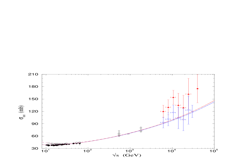
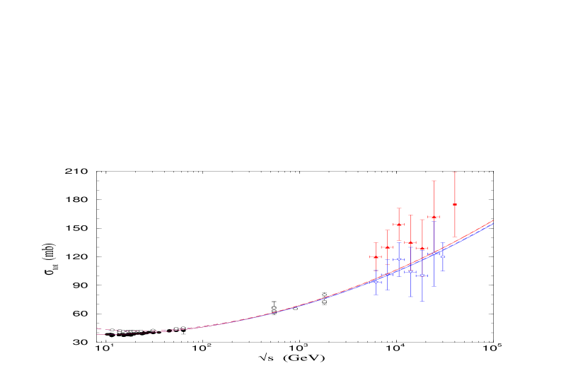
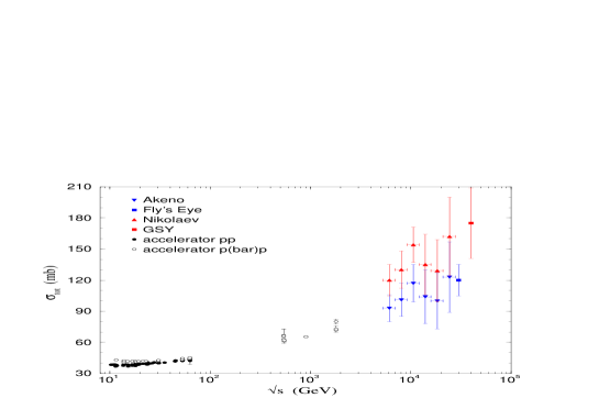
In the case of accelerator experiments, data on $\sigma_{tot}$ from $pp$ and $\overline{p}p$ total cross sections and also estimations of the $\rho$ parameter have been accumulated for a long time. The data sets, compiled and analyzed by the Particle Data Group, have become a standard reference and are available (also readable files) at http://pdg.lbl.gov. Recent analysis has shown that general fits are stable for $\sqrt{s}$ above $\sim$ 9 GeV [3]. For this reason in this work we make use of these sets for energies above $10$ GeV and in our analysis the statistic and systematic errors were added linearly. The total cross section data are shown in Fig. 1.

B Cosmic ray information

The extraction of the proton-proton total cross section from cosmic ray experiments is based on the determination of the proton-air production cross section from analysis of extensive air showers. Detailed review on the subtle involved may be found in References [4] and [5]. Here we only recall the two main steps, stressing the model dependence involved.

The first step concerns the determination of the proton-air production cross section, namely, the “inelastic cross section in which at least one new hadron is produced in addition to nuclear fragments” [5]. This is obtained by the formulas

$$\sigma_{p-air}^{prod}(mb)=\frac{2.4\times 10^{4}}{\lambda_{p-air}(g/cm^{2})},\qquad\lambda_{p-air}(g/cm^{2})=\frac{\lambda_{att}}{k},$$ (2)

where, $\lambda_{p-air}$ is the interaction length of protons in the atmosphere, $\lambda_{att}$ the shower attenuation length and $k$ is a measure of the dissipation of the energy through the shower. The $\lambda_{att}$ is a experimental quantity determined through the $\chi_{max}$ Attenuation Method or the Zenith Angle Attenuation Technique [6]. On the other hand, the parameter $k$ is obtained through Monte Carlo simulation and so is strongly model dependent [5].

In a second step $\sigma_{pp}^{tot}$ is obtained from $\sigma_{p-air}^{prod}$ through the Multiple Diffraction Formalism by Glauber and Matthiae [7] and taking account of the screening correction ($\Delta\sigma$):

$$\sigma_{p-air}^{tot}=\sigma_{p-air}^{el}+\sigma_{p-air}^{prod}+\sigma_{p-air}^{q-el}+\sigma_{p-air}^{diff}+\Delta\sigma$$ (3)

Two important inputs at this point are the nucleon distribution function and the slope parameter $B$, necessary in the parametrization of the proton-proton scattering amplitude:

$$F_{pp}(s,q)\propto\exp\{\frac{-B(s)q^{2}}{2}\},$$ (4)

where $q^{2}$ is the four-momentum transfer squared.

The results presently available from cosmic ray experiments cover the region $\sqrt{s}\sim 6-40$ TeV and are characterized by discrepancies, mainly due to the model dependence of $k$ and $B(s)$. However, we can classify these results according to the degree of consistence of the analysis and, simultaneously, by value of the total cross section extracted, as explained in what follows.

From one hand the results usually quoted in the literature concern those obtained by the Fly’s Eye Collaboration in 1984 [8] and Akeno (Agasa) Collaboration in 1993 [9]. In the first case, the authors used $k=1.6$ and a relation of proportionality between $B$ and $\sigma_{pp}^{tot}$ as predicted by the Geometrical Scaling model [10]. At $\sqrt{s}=30$ TeV the cross sections results are [8]:

$$\sigma_{p-air}^{prod}=540\pm 50{\rm\ mb}\qquad\sigma_{pp}^{tot}=122\pm 11{\rm\ mb}$$ (5)

The Akeno Collaboration used $k=1.5$ and the Durand and Pi method [11, 12] to extract the proton-proton cross sections in the region $\sqrt{s}\sim 6-20$ TeV. The results are displayed in Fig. 1 together with the Fly’s Eye value at $\sqrt{s}=30$ TeV.

On the other hand, in 1987 Gaisser, Sukhatme, Yodh (GSY) making use of the Fly’s Eye result for $\sigma_{p-air}^{prod}$ and the Chou - Yang prescription for $B(s)$ obtained at $\sqrt{s}=40$ TeV [13]:

$$\sigma_{pp}^{tot}=175_{-27}^{+40}$$ (6)

In 1993, Nikolaev claimed that the Akeno results should be corrected in order to take account of the differences between absorption and inelastic cross sections, leading to an increase of the published results by $\approx 30$ mb [14].

All these cosmic ray estimates together with the accelerator results are displayed in Fig 1 and show that, despite of the large error bars, we can identify two distinct set of estimations: one represented by the results of the Fly’s Eye Collaboration together with those by the Akeno Collaboration; the other by the results of Gaisser, Sukhatme, Yodh with those by Nikolaev. Taken separately these two sets suggest different behaviors for the increase of the total cross section.

At this point it should be stressed that the Fly’s Eye Collaboration used the Geometrical Scaling hypothesis, which is violated even at the collider energy and so this result is certainly wrong. Durand and Pi asserted in Ref. [12] that their results presented in [11], and used by the Akeno Collaboration, should be disregarded due to a wrong approximation. On the other hand, to our knowledge, the results by Gaisser, Sukhatme, Yodh and Nikolaev have never been critized in the literature. But we must yet take account of the model dependence involved as discussed in [4, 5].

For the above reasons we shall quantitatively investigate the statistical determination of possible lower or upper limits in the increase of the total cross section, associated with the results by Akeno - Fly’s Eye and Nikolaev - GSY, respectively. To this end we consider two ensembles of data, above $10$ GeV, defined by:

  Ensemble I:

$\overline{p}p$ accelerator data and $pp$ accelerator data + Akeno + Fly’s Eye.

  Ensemble II:

$\overline{p}p$ accelerator data and $pp$ accelerator data + Nikolaev + GSY.

FIG. 1.: Total cross sections ($pp$ and $\overline{p}p$ above $\sqrt{s}=10$ GeV): accelerator data and cosmic ray information available.

III Analytical Approach

A Analyticity relations

For $pp$ and $\overline{p}p$ scattering, crossing symmetry is expressed by

$$\sigma_{\pm}(s)=\frac{\sigma_{tot}^{pp}\pm\sigma_{tot}^{p\overline{p}}}{2}$$ (7)

and Analyticity allows to connect $\sigma_{tot}(s)$ and $\rho(s)$ through two compact and symmetric formulas,

$$\rho^{pp}\sigma_{tot}^{pp}(s)=E(\sigma_{+})+O(\sigma_{-}),$$ (8)

$$\rho^{p\overline{p}}\sigma_{tot}^{p\overline{p}}(s)=E(\sigma_{+})-O(\sigma_{-}),$$ (9)

where, $E(\sigma_{+})$ and $O(\sigma_{-})$ are analytic transforms relating real and imaginary parts of $E$ven ($+$) and $O$dd ($-$) amplitudes, respectively. They are generally represented by integral formulas (Integral Dispersion Relations) and in the case of one subtraction they are expressed by [2]

$$E_{int}(\sigma_{+})\equiv\frac{K}{s}+\frac{2s}{\pi}\int_{s_{o}}^{\infty}\mathrm{d}s^{\prime}\left[\frac{1}{s^{\prime 2}-s^{2}}\right]\sigma_{+}(s^{\prime})=\frac{ReF_{+}(s)}{s},$$ (10)

$$O_{int}(\sigma_{-})\equiv\frac{2}{\pi}\int_{s_{o}}^{\infty}\mathrm{d}s^{\prime}\left[\frac{s^{\prime}}{s^{\prime 2}-s^{2}}\right]\sigma_{-}(s^{\prime})=\frac{ReF_{-}(s)}{s},$$ (11)

where $K$ is the subtraction constant.

At high energies we can take the limit $s_{0}\rightarrow 0$ and in this case they are equivalent to derivative forms given formally by [15, 16, 17, 18, 19]

$$E_{der}(\sigma_{+})\equiv\frac{K}{s}+\tan\left[\frac{\pi}{2}\frac{d}{d\ln s}\right]\sigma_{+}(s)=\frac{ReF_{+}(s)}{s},$$ (12)

$$O_{der}(\sigma_{-})\equiv\tan\left[\frac{\pi}{2}(1+\frac{d}{d\ln s})\right]\sigma_{-}(s)=\frac{ReF_{-}(s)}{s}.$$ (13)

Operationally these expressions may be evaluated through the expansions [16, 17, 19]:

$$E_{der}(\sigma_{+})-\frac{K}{s}=\left[\frac{\pi}{2}\frac{d}{d\ln s}+\frac{1}{3}\left(\frac{\pi}{2}\frac{d}{d\ln s}\right)^{3}+\frac{2}{15}\left(\frac{\pi}{2}\frac{d}{d\ln s}\right)^{5}+...\right]\sigma_{+}(s),$$ (14)

$$O_{der}(\sigma_{-}) = -\frac{2}{\pi}\int\left\{\frac{d}{d\ln s}\left[\cot\left(\frac{\pi}{2}\frac{d}{d\ln s}\right)\right]\sigma_{-}(s)\right\}d\ln s$$ (15)

$$= -\frac{2}{\pi}\int\left\{\left[1-\frac{1}{3}\left(\frac{\pi}{2}\frac{d}{d\ln s}\right)^{2}-\frac{1}{45}\left(\frac{\pi}{2}\frac{d}{d\ln s}\right)^{4}-...\right]\sigma_{-}(s)\right\}d\ln s$$ (16)

With this approach, $\rho(s)$ may be determined through suitable input parametrizations for the total cross sections. In this communication we shall use two different choices for these inputs:

$\bullet$ Donnachie-Landshoff (DL)

The Donnachie-Landshoff parametrization for the total cross sections are expressed by [20]

$$\sigma_{tot}^{pp}(s)=Xs^{\epsilon}+Ys^{-\eta}\qquad\quad\sigma_{tot}^{p\overline{p}}(s)=Xs^{\epsilon}+Zs^{-\eta}$$ (17)

where, originally, $X=21.7$ mb, $Y=56.08$ mb, $Z=98.39$ mb, $\epsilon=0.0808$, $\eta=0.4525$.

For this parametrization Eqs. (8) and (9) reads

$$\rho^{pp}=\frac{1}{\sigma_{tot}^{pp}}\left\{\frac{K}{s}+\left[X\tan(\frac{\pi\epsilon}{2})\right]s^{\epsilon}+\left[\frac{(Y-Z)}{2}\cot(\frac{\pi\eta}{2})-\frac{(Y+Z)}{2}\tan(\frac{\pi\eta}{2})\right]s^{-\eta}\right\}$$ (18)

$$\rho^{\overline{p}p}=\frac{1}{\sigma_{tot}^{\overline{p}p}}\left\{\frac{K}{s}+\left[X\tan(\frac{\pi\epsilon}{2})\right]s^{\epsilon}+\left[\frac{(Z-Y)}{2}\cot(\frac{\pi\eta}{2})-\frac{(Y+Z)}{2}\tan(\frac{\pi\eta}{2})\right]s^{-\eta}\right\}$$ (19)

We see that this choice implies

$$\Delta\sigma=\sigma^{\overline{p}p}_{tot}(s)-\sigma^{pp}_{tot}(s)=(Z-Y)s^{-\eta}\rightarrow 0\quad{\rm(asymptotically)}$$ (20)

$\bullet$ Kang-Nicolescu (KN)

The parametrizations for the total cross sections under the possibility of a maximal Odderon contribution are given by [17]

$$\sigma^{pp}_{tot}(s)=A_{1}+B_{1}\ln s+k\ln^{2}s,\qquad\sigma^{\overline{p}p}_{tot}(s)=A_{2}+B_{2}\ln s+k\ln^{2}s+2Rs^{-1/2}$$ (21)

and Eqs. (8) and (9) give

$$\rho^{pp}=\frac{1}{\sigma_{tot}^{pp}}\left\{\frac{K}{s}+\frac{\pi}{2}\left(\frac{B_{1}+B_{2}}{2}\right)+\left(\pi k+\frac{A_{2}-A_{1}}{\pi}\right)\ln s+\left(\frac{B_{2}-B_{1}}{2\pi}\right)\ln^{2}s-2Rs^{-1/2}\right\}$$ (22)

$$\rho^{\overline{p}p}=\frac{1}{\sigma_{tot}^{\overline{p}p}}\left\{\frac{K}{s}+\frac{\pi}{2}\left(\frac{B_{1}+B_{2}}{2}\right)+\left(\pi k-\frac{A_{2}-A_{1}}{\pi}\right)\ln s-\left(\frac{B_{2}-B_{1}}{2\pi}\right)\ln^{2}s\right\}$$ (23)

In this case we have

$$\Delta\sigma=\sigma^{\overline{p}p}_{tot}(s)-\sigma^{pp}_{tot}(s)=(A_{2}-A_{1})+(B_{2}-B_{1})\ln s+2Rs^{-1/2}\rightarrow\Delta A+\Delta B\ln s$$ (24)

so that if $\Delta A\not=0$ and/or $\Delta B\not=0$ then, asymptotically, $\Delta\sigma\not=0$.

IV Fits and Results

As referred to before, we shall consider several cases: for both parametrizations (DL and KN) we perform independent and simultaneous fits to $\sigma_{tot}(s)$ and $\rho(s)$ by considering the two ensembles I and II, separately.

In the individual procedure we first fit the $\sigma_{tot}$ data through Eqs. (10) (DL) or (11) (KN) and then fit the $\rho$ data by letting free the subtraction constant $K$ only; in the simultaneous procedure the subtraction constant $K$ is a free parameter in the overall fit to both quantities. The fits were performed through the CERN-minuit routine.

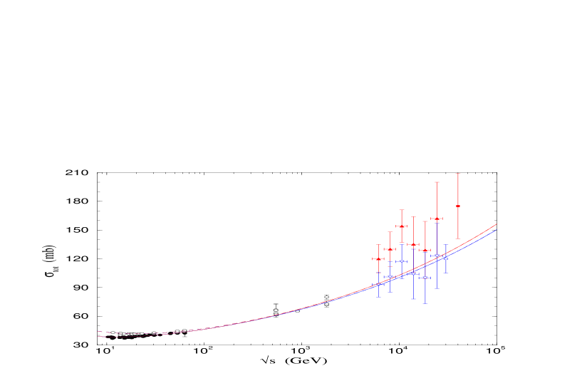
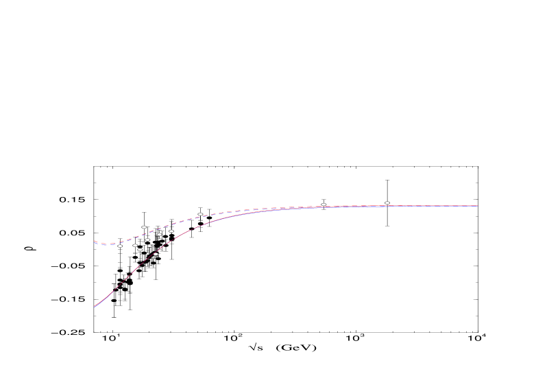
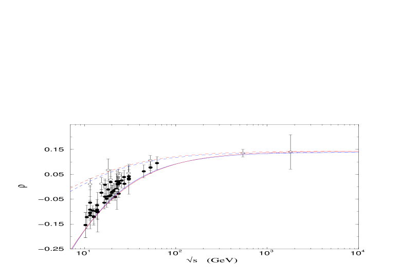
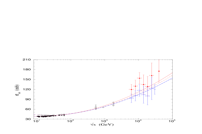
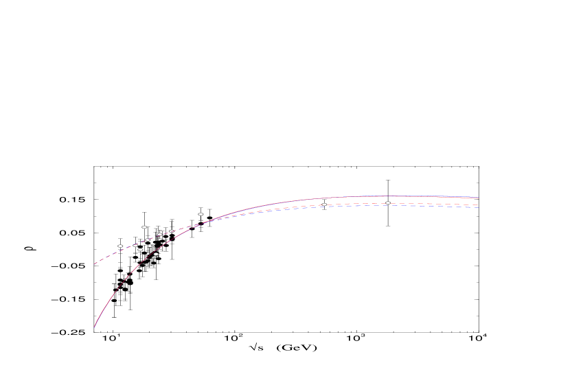
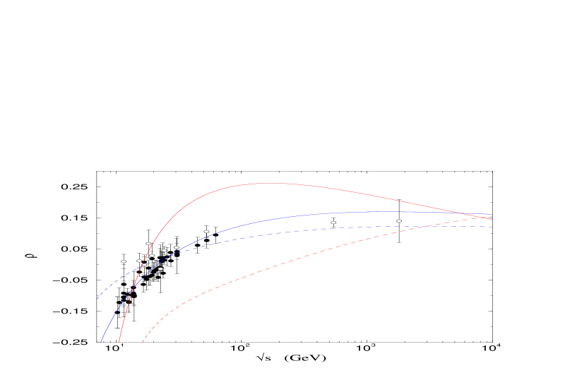
The results with the DL parametrization are shown in Figs. 2 and 3 and the statistical information are displayed in Table 1. Those with the KN parametrization in Figs. 4 and 5 and Table 2.

V Conclusions and final Remarks

From Tables 1 and 2 and Figures 2 to 5 we are lead to the following main conclusions:

$\bullet$ Ensembles I and II

In general, the results with ensembles I and II do not differ substantially and the cosmic ray information in ensemble II (Nikolaev and GSY) are not described in all the cases. Certainly this is due to the small number of points and the large error bars as compared with the accelerator data and also to the choices for the parametrizations. However noticeable differences occur with the Kang Nicolescu parametrization (Figures 4 and 5).

$\bullet$ Simultaneous and individual fits

The best statistical results are obtained through the simultaneous fits. For example, in the case of DL parametrization, $\chi^{2}/d.o.f.\sim 1.0$ (simultaneous) and $\sim 1.7$ (individual for $\rho$). This is expected since in the simultaneous case we have more statistical information (degree of freedom).

On the other hand simultaneous fits constraint the rise of the total cross section. For example, in the case of the DL parametrization with ensembles I and II we obtained:

$\epsilon_{indi}^{I}\sim 0.088\rightarrow\epsilon_{simul}^{I}\sim 0.083$ (reduction $\sim 6\%$)

$\epsilon_{indi}^{II}\sim 0.091\rightarrow\epsilon_{simul}^{II}\sim 0.084$ (reduction $\sim 8\%$)

As commented before, $\sigma_{tot}$ and $\rho$ do not have the same status as physical quantities since the $\rho$ value is model dependent. Therefore we understand that the simultaneous fit may led to erroneous predictions for $\sigma_{tot}$ in the asymptotic region (underestimation).

$\bullet$ Upper bounds for the soft Pomeron intercept

The upper bound was obtained with ensemble II in the case of individual fits

$1+\epsilon=1.091\pm 0.003\qquad 1-\eta=0.65\pm 0.03$

$\bullet$ Odderon

From Tables 3 and 4, $\Delta A$ and $\Delta B$ $\sim$ $0$ in 3 cases and the only exception is for individual fits with ensemble II, for which $\Delta A=5\pm 3$ and $\Delta B\sim 0$. This predicts a crossing with $\sigma_{tot}^{pp}$ becoming higher than $\sigma_{tot}^{\overline{p}p}$. However, in this case $\rho$ is not described as shown in Fig. 5. We conclude that our results do not favor the Odderon possibility.

We observe that a similar and interesting analysis, taking quantitative account of the cosmic ray information, has been presented in this Workshop by Carlos Avila [21]. Although the technical approach is different the global results are in agreement with those presented here and in Ref. [19].

Acknowledgments

Work supported by FAPESP and CNPq, Brazil. M.J.M. is thankful to Prof. Alberto Santoro and the organizers of this excellent Workshop and to U. Maor and C. Avila for useful discussions during the meeting.

TABLE I.: Simultaneous and individual fits to $\sigma_{tot}$ and $\rho$ for Ensembles I and II with the DL parametrization.

Fit:	Simultaneous		Individual
Ensemble:	I	II	I	II
N. points	$165$	$165$	$102$	$102$
$\chi^{2}/d.o.f.$	$0.84$	$0.98$	$0.76$	$0.96$
$X$ (mb)	$21.4\pm 0.4$	$21.1\pm 0.4$	$20.0\pm 0.7$	$19.3\pm 0.7$
$Y$ (mb)	$67\pm 6$	$67\pm 5$	$48\pm 5$	$46\pm 5$
$Z$ (mb)	$114\pm 11$	$112\pm 11$	$75\pm 10$	$70\pm 9$
$\eta$	$0.48\pm 0.02$	$0.47\pm 0.02$	$0.37\pm 0.04$	$0.35\pm 0.03$
$\epsilon$	$0.083\pm 0.002$	$0.084\pm 0.002$	$0.088\pm 0.003$	$0.091\pm 0.003$
$K$	$306\pm 54$	$307\pm 54$	-	-
N. points ($\rho$)	-	-	$63$	$63$
$\chi^{2}/d.o.f.$	-	-	$1.55$	$1.84$
$K$	-	-	$235\pm 32$	$245\pm 32$

TABLE II.: Simultaneous and individual fits to $\sigma_{tot}$ and $\rho$ for Ensembles I and II with the KN parametrization.

Fit:	Simultaneous		Individual
Ensemble:	I	II	I	II
N. points	165	165	102	102
$\chi^{2}/d.o.f.$	$0.77$	$0.86$	$0.78$	$0.91$
$A_{1}$ (mb)	$44.4\pm 0.7$	$45.0\pm 0.7$	$45\pm 1$	$47\pm 1$
$A_{2}$ (mb)	$44.5\pm 0.7$	$45.1\pm 0.7$	$45\pm 3$	$52\pm 3$
$B_{1}$ (mb)	$-2.9\pm 0.2$	$-3.1\pm 0.2$	$-2.9\pm 0.3$	$-3.6\pm 0.4$
$B_{2}$ (mb)	$-2.9\pm 0.2$	$-3.1\pm 0.2$	$-2.9\pm 0.6$	$-4.2\pm 0.6$
$k$ (mb)	$0.33\pm 0.01$	$0.35\pm 0.01$	$0.33\pm 0.06$	$0.39\pm 0.03$
$R$ (mb GeV)	$25.3\pm 0.9$	$25.4\pm 0.9$	$24\pm 7$	$12\pm 7$
$K$	$-72\pm 46$	$-63\pm 46$	-	-
N. points ($\rho$)	-	-	63	63
$\chi^{2}/d.o.f.$	-	-	$1.05$	$35.2$
$K$	-	-	$-198\pm 32$	$-1369\pm 32$

FIG. 2.: Fits to $\sigma_{tot}$ with the DL parametrization: $pp$ (solid) and $\overline{p}p$ (dashed) and ensembles I (blue) and II (red). Simultaneous (up) and individual (down).

FIG. 3.: Fit to $\rho$ with the DL parametrization: $pp$ (solid) and $\overline{p}p$ (dashed) and ensembles I (blue) and II (red). Simultaneous (up) and individual (down).

FIG. 4.: Fits to $\sigma_{tot}$ with the KN parametrization: $pp$ (solid) and $\overline{p}p$ (dashed) and ensembles I (blue) and II (red). Simultaneous (up) and individual (down).

FIG. 5.: Fit to $\rho$ with the KN parametrization: $pp$ (solid) and $\overline{p}p$ (dashed) and ensembles I (blue) and II (red). Simultaneous (up) and individual (down).

REFERENCES

- [1] G. Matthiae, Rep. Prog. Phys. 57, 743 (1994).
- [2] M. M. Block and R. N. Cahn, Rev. Mod. Phys. 57, 563 (1985).
- [3] J.R. Cudell, V. Ezhela, K. Kang, S. Lugovsky, N. Tkachenko, in Proc. VIIIth Blois Workshop - Int. Conf. Elastic and Diffractive Scattering, edited by V.A. Petrov and A.V. Prokudin (World Scientific, Singapore, 2000) p. 251-258; Phys. Rev. D61, 034019 (2000), Erratum Phys. Rev. D63, 059901 (2001).
- [4] T.K. Gaisser, Nucl. Phys. B (Proc. Suppl.) 12, 172 (1990).
- [5] R. Engel, T. K. Gaisser, P. Lipari, and T. Stanev, Phys. Rev. D 58, 014019 (1998).
- [6] P. Sokolsky, ”Introduction to Ultrahigh Energy Cosmic Ray Physics” - Frontiers in Physics (Addison Wesley, 1989).
- [7] R.J. Glauber, G. Matthiae, Nucl. Phys. B21, 135 (1970).
- [8] Fly’s Eye Collaboration (R. M. Baltrusaitis et al.), Phys Rev. Lett. 52, 1380 (1984).
- [9] Akeno Collaboration (H. Honda et al., Phys. Rev. Lett. 70, 525 (1993).
- [10] J. Dias de Deus, Nucl. Phys. B59, 231 (1973); A.J. Buras and J. Dias de Deus, Nucl. Phys. B71, 481 (1974).
- [11] L. Durand and H. Pi, Phys. Rev. D 38, 78 (1988)
- [12] L. Durand and H. Pi, Nucl. Phys. B (Proc. Suppl.) 12, 379 (1990).
- [13] T.K. Gaisser, U.P. Sukhatme, and G.B. Yodh, Phys. Rev. D 36, 1350 (1987).
- [14] N.N. Nikolaev, Phys. Rev. D 48, R1904 (1993).
- [15] N.V. Gribov and A.A. Migdal, Sov J. Nucl. Phys. 8, 583 (1969); J. B. Bronzan, Argonne Symposium on the Pomeron, ANL/HEP-7327, 33 (1973); J. D. Jackson, 1973 Scottish Summer School, LBL-2079, 39 (1973).
- [16] J. B. Brozan, G. L. Kane, and U. P. Sukhatme, Phys. Lett. B49, 272 (1974).
- [17] K. Kang and B. Nicolescu, Phys. Rev. D 11, 2461 (1975).
- [18] M.J. Menon, A.E. Motter, and B.M. Pimentel, Phys. Lett. B 451, 207 (1999); in 1997 - XVIII Brazilian National Meeting on Particles and Fields, edited by O. J. P. Éboli et al. (SBF, São Paulo, 1998) pp. 548-552.
- [19] R.F. Ávila, E.G.S. Luna, M.J. Menon, Braz. J. Phys. 31, 567 (2001), arXiv:hep-ph/0105065.
- [20] A. Donnachie and P. V. Landshoff, Z. Phys. C 2, 55 (1979); Phys. Lett. B 387, 637 (1996).
- [21] C. Avila, “Total Hadronic Cross Sections at the LHC and VLHC Energies”, these proceedings.