Prompt Multi-Gluon Production in High Energy Collisions
from Singular Yang-Mills Solutions

Abstract

We study non-perturbative parton-parton scattering in the Landau method using singular O(3) symmetric solutions to the Euclidean Yang-Mills equations. These solutions combine instanton dynamics (tunneling) and overlap (transition) between incoming and vacuum fields. We derive a high-energy solution at small Euclidean times, and assess its susequent escape and decay into gluons in Minkowski space-time. We describe the spectrum of the outgoing gluons and show that it is related through a particular rescaling to the Yang-Mills sphaleron explosion studied earlier. We assess the number of incoming gluons in the same configuration, and argue that the observed scaling is in fact more general and describes the energy dependence of the spectra and multiplicities at all energies. Applications to hadron-hadron and nucleus-nucleus collisions are discussed elsewhere.

]

I Introduction

Tunneling phenomena related with topology of Yang-Mills fields are described semiclassically by instantons [1, 2]. Some manifestations of these effects related with explicit breaking of U(1) and spontaneous breaking of $SU(N_{f})$ chiral symmetries are by now understood in significant detail due to strong ties to hadronic phenomenology and lattice studies, see e.g.[3] for a review.

We know much less about the role of instantons in cross sections of various high-energy reactions. Such studies got considerable attention in the early 90’s, when baryon-number violating processes through instantons in the standard model have been actively discussed [4, 5]. These studies were extended to hard QCD processes with small-size instantons, and there are still attempts to see their effects on multi-jet production at HERA (for recent review see [7]).

Recently [8, 9] it was suggested that nonperturbative configurations composed of instanton/antiinstanton play an important role in parton-parton scattering amplitudes at high-energy, and may account for most of the soft pomeron slope and intercept. The logarithmic rise of the inelastic cross-section was shown to follow from coherent multiple gluon production as described by the semiclassical field following from an interacting instanton-antiinstanton configuration. This mechanism was shown to be the same for $pp$ and $\overline{p}p$ [8]: so no odderon appears in the classical limit. At low energy transfer in the center of mass, the interaction is dipole, and accounts for the rise in the partial cross section from first principles. At intermediate and large energy transfer, the dipole approximation is not reliable as strong instanton-antiinstanton interactions set in together with unitarity constraints [5, 8].

It was realized then that unlike perturbative processes, for which production of each subsequent gluon is associated with a power of small coupling constant, in instanton-induced processes the cross section rises with a number of produced gluons reaching a maximum at some parametrically large value $N\approx 1/\alpha(\rho)$. The physical reason for this is that specific coherent clusters of gauge field are produced instead of independent gluons. In a recent paper [10] the properties of minimal clusters of such kind were discussed: the clusters themselves were identified via constrained minimization of the Yang-Mills energy, with fixed size and Chern-Simon number, and their subsequent real time evolution have been studied both numerically and analytically.

However, in real collisions the Yang-Mills energy or action of the final state is only one of the contributing factors. Another crucial factor is the overlap between the initial system of colliding gluons and the instanton, or whatever the tunneling path is. A particularly useful way [11] to treat both semiclassical factors from first principles together, and enforce the unitarity constraints is to use a semiclassical approximation to the partial cross section based on an adaptation of the Landau formula for overlaping matrix elements in terms of singular field configurations. The occurence of a singularity is an essential feature of the Euclidean field configuration that interpolates between the vacuum at $t=-\infty$ with zero energy, and the escape point at $t=0$ with finite energy.

Diakonov and Petrov [6] used this approach (Landau method) to rederive the low-energy limit of the amplitude, and obtain a new result in the high-energy limit. Although they have not worked out the gauge configuration at small times explicitly, they were still able to assess the corresponding action, tunneling time and energy, to predict the behavior of the pertinent cross section at high-energy. A comparison of the low- and high-energy limits, has confirmed that the cross section has a maximum near the sphaleron energy with a value that is close to the square-root of the cross section near zero-energy.

The aim of the present paper is to analyze further the singular gauge configurations at the escape time $t=0$. Following [6] we start with the high-energy limit and show how one can find the gauge configuration at the turning point which is the produced gluon cluster at $t=0$. It turns out that this configuration can be related to minimal YM sphalerons [10] by a particular scaling law, containing a power of $Q/M_{s}$. We show that the subsequent evolution (explosion) in real time of these clusters can also be derived, thereby generalizing recent work [10] by our rescaling. The resulting spectrum of gluons and their multiplicity are readily obtained. We argue that the prescribed scaling law is valid not only at high energies, above the sphaleron mass, but in fact at $all$ energies.

In section 2 we introduce the standard notations for the spherically symmetric gauge configurations used. In section 3, we recall the key points in assessing the inelastic parton-parton scattering cross-section in the eikonal approximation. In section 4, we show that the singular gauge configurations at the escape points follow from the sphaleron point for all energies through a pertinent rescaling, which is our main result. In sections 5, we assess the number of incoming and outgoing gluons per sphaleron for fixed center of mass energy in the semiclassical approximation. Our conclusions are in section 6. The Appendices contain a number of useful results including a stability analysis of the escaping configurations under perturbative light pair-decay.

II O(3) Symmetric Yang-Mills

We consider the QCD Yang-Mills theory wherein all dimensions are rescaled away by the sphaleron (antisphaleron) mass $M_{S}$,

$$M_{S}=\frac{1}{4\alpha}\,\int_{0}^{\infty}\,dx\,x^{2}\frac{96\rho^{4}}{(x^{2}+\rho^{2})^{4}}=\frac{3\pi}{4\,\alpha\,\rho}\,\,,$$ (1)

unless specified otherwise. In the vacuum $\alpha\approx 0.3$, $\rho\approx 1/3$ fm with typically $M_{S}\approx 3$ GeV. In the scattering process, the sphaleron (antisphaleron) size $\rho$ may change. We work mainly in temporal gauge. The YM potential ${\bf V}$, kinetic energy ${\bf K}$ and Chern-Simons number ${\bf N}$ are

$${\bf V}=\frac{M_{S}}{4\pi\,\alpha}\,\int d\vec{x}\,\frac{1}{4}\,(F_{ij}^{a})^{2}$$ (2)

$${\bf K}=\frac{M_{S}}{4\pi\,\alpha}\,\int d\vec{x}\,\frac{1}{2}\,(\dot{A}_{i}^{a})^{2}$$ (3)

$${\bf N}=\frac{1}{16\pi^{2}}\,\int d\vec{x}\,\epsilon_{ijk}\,(A_{i}^{a}\,\partial_{j}\,A_{k}^{a}+\frac{1}{3}\epsilon_{abc}\,A_{i}^{a}\,A_{j}^{b}\,A_{k}^{c})\,\,,$$ (4)

where we have ignored quarks for simplicity.

In parton-parton scattering with large $\sqrt{s}$, the incoming kinematics boils down to an eikonalized cross section as in (14) with a partial cross section $\sigma\,(Q)$ with $Q\approx M_{S}\ll\sqrt{s}$. In the center of mass it is reasonable to consider the gluonic configurations that maximizes $\sigma\,(Q)$ to possess higher symmetries than completely arbitrary fields. Here we take them to have spherical $O(3)$ symmetry of the sphaleron

$$A_{i}^{a}(\vec{x},t)= +\epsilon_{aij}\,n_{i}\,(1-A(x,t))/x$$ (7)

$$+(\delta_{ai}-n_{a}n_{i})\,B(x,t)/x$$

$$+n_{a}n_{i}\,C(x,t)/x$$

where $n_{i}=\vec{x}_{i}/x$ is a unit 3-vector, and $|\vec{x}|=x\geq 0$ a radial variable. Since we are interested in singular gauge fields, we assume the three 2-dimensional independent functions $A,\,B,\,C$ to be continuous and differentiable everywhere in Euclidean space, except at $x=0$ where a singularity will be located for fixed times $\pm T/2$. In terms of (7) the Euclidean action

$$S=\int dt\,({\bf K}+{\bf V})$$ (8)

reads

$$S=\frac{1}{\alpha}\int\,dt\,\int_{0}^{\infty}\,dx(\dot{A}^{2}+\dot{B}^{2}+\frac{1}{2}\,\dot{C}^{2}+{A^{\prime}}^{2}+{B^{\prime}}^{2}$$ (9)

$$+\frac{(A^{2}+B^{2}-1)^{2}}{2x^{2}}+\frac{C^{2}(A^{2}+B^{2})}{x^{2}}+\frac{2C(A^{\prime}B-AB^{\prime})}{x})$$ (10)

where the time variable has been rescaled through $t\,M_{S}\rightarrow t$, in (10). The integration interval is to be specified below in the presence of a time-singularity. Note that the energy

$$-Q={\bf K}-{\bf V}$$ (11)

where in Euclidean space $-{\bf V}$ plays the role of the potential. For self-dual configurations $Q=0$. The Chern-Simons number is

$${\bf N}=\frac{1}{2\pi}\int_{0}^{\infty}\,dx\,\left(A^{\prime}B-B^{\prime}A+\frac{C}{x}(A^{2}+B^{2}-1)\right)\,\,.$$ (12)

The dual to the O(3) ansatz used here that maps on the antisphaleron follows similar reasoning and results as shown in Appendix A. The difference is a negative ${\bf N}$.

III The Evolving Views on Non-perturbative High Energy Processes

In this work we discuss semi-hard parton-parton processes at fixed $\sqrt{-t}\sim 1\,{\rm GeV}\ll\sqrt{s}$, using nonperturbative QCD gauge configurations related to topological tunneling. The original approach [4] wich we followed in [8] was based on semiclassical instanton solution in the amplitude. To leading order in the small tunneling or diluteness factor of the typical density and size of instantons in the vacuum, $\kappa=n_{\rm inst}\rho^{4}\approx 10^{-2}$ (see e.g.[3] for details), the inelastic cross section reads

$$\sigma_{\rm in}(s,t)\approx \,{\bf C}\,\pi\,\rho^{2}\,{\rm ln\,s}\,\int\,dq_{1\perp}\,dq_{2\perp}\,\,{\bf K}(q_{1\perp},q_{2\perp},t)$$ (14)

$$\times\,\int^{\infty}_{(q_{1\perp}+q_{2\perp})^{2}}\,dQ^{2}\,\kappa^{2}\,{\bf B}(Q)$$

where ${\bf K}$ is a pertinent instanton form factor at fixed $-t\ll s$, containing through-going partons in the form of Wilson lines. $\kappa$ appears squared since the cross section involves the squared amplitude. B(Q) is the partial multi-gluon cross section for fixed $Q^{2}\ll s$ and ${\bf C}$ an overall constant which accounts for both the instanton and antiinstanton contributions to the initial state. To exponential accuracy

$$\kappa^{2}{\bf B}(Q)\approx{\rm Im}\int\,dT\,e^{QT-{\bf S}(T)}$$ (15)

where ${\bf S}(T)$ is the effective action describing instanton-antiinstanton interaction for a time-separation $T$, which is defined to reduce to twice the free instanton action at large $T$. This effective action, also known as the “holy grail function”, is supposed to sum up contributions of any number of produced gluons. For small $Q$ or large $T$, the dipole approximation is valid and (15) rises exponentially with $Q$ [4]. However, as emphasized first by Zakharov [5] the unitarity constraints on the partial cross section requires ${\bf B}(Q)$ to fall at large $Q$. Shifman and Maggiore [5] argued that the unitarization could be qualitatively enforced by resumming chains of instantons and antiinstantons. In [8] we followed this idea and indeed found that the dominant contribution to (15) occurs at the sphaleron point for which ${\bf B}(M_{S})\approx 1/\kappa$. Hence,

$$\sigma_{\rm in}(s,t)\approx {\bf C}\,\pi\rho^{2}\,\kappa\,{\rm ln\,s}\,\,\int\,dq_{1\perp}\,dq_{2\perp}\,\,{\bf K}(q_{1\perp},q_{2\perp},t)\,\,.$$ (16)

The rise in the partial inelastic cross section due to the production of the Yang-Mills (YM) sphaleron , results into an increase of the inelastic cross section by one power of the diluteness factor $\kappa$, or about a 100-fold increase [8].

This qualitative solution of the problem implies however that the maximal cross section does not correspond to a well-separated instanton-antiinstanton pair, but rather to a close pair with $T\approx\rho$ whereby half of the asymptotic action is annihilated. Detailed studies of close instanton-antiinstanton configurations of such kind have been made recently in [10]. An important new element of that paper was the emphasis on the t=0 3-plane, treated as a unitarity cut and explicitly describing the turning (escaping to Minkowski space-time) gauge field configuration. Although this paper was not dealing with the cross section calculation, following its logic one should e.g. modify the form-factor K in (14) by using Wilson lines in a half-instanton-antiinstanton field as described for instance by the Yung ansatz.

However, even this solution of the problem would not be ideal, as it treats independently two small semiclassical factors, the instanton-antiinstanton interaction S in the vacuum and the form-factor K. The idea behind the Landau method is to treat these semiclassical contributions simultaneously. The essentials of the method are as follows (more details can be found in [6]): In quantum mechanics the overlap between the ground state and a highly excited state can be rewritten as a difference of two shortened actions for a pair of paths with energy 0 and $Q$ respectively. The corresponding integrals interpolate between the turning points and the singularity at infinity. The location of the singularity of the gauge configuration plays the role of such an infinity. Specific Euclidean paths, used originally in [11, 6], have singularities in the $A_{\mu}$ field located at r=0 and time $\mp T/2$, see fig.1. Outside the region marked by the dashed lines the solution is the universal singular instanton, describing the ground state. Between the dashed lines it is supposed to be the (so far missing) energy-Q solution: both solutions join smoothly at the dashed lines. Our aim is to find the interpolating solution, at least approximately, and investigate at $t=0$ the internal field structure of relevant turning states. Their subsequent evolution will eventually lead to predictions of what is actually produced in the collision.

FIG. 1.: Euclidean pace-time (r,t) plane. The circles indicate the location of the gauge singularities, and the vertical lines show where the 0-energy and Q-energy solution are joined.

IV More details on Singular Yang-Mills

A Singular fields: $|t|>T/2$

The branch of the field that interpolates between the vacuum at $t=-\infty$ and the singularity at $t=-T/2$ with zero energy and minimizes (8) is an instanton. The conjugate branch is an an antiinstanton and interpolates between the singularity at $t=+T/2$ and the vacuum at $t=+\infty$. In covariant gauge, both branches are given by

$$A_{\mu}^{a}(x(\pm))= 2\,\eta_{\mu\nu}(\pm)\,x_{\nu}(\pm)\Phi(x^{2}(\pm))$$ (17)

$$= \frac{2\,\eta_{\mu\nu}^{a}(\pm)\,x_{\nu}(\pm)\,\rho^{2}}{(\rho^{2}-x^{2}(\pm))\,x^{2}(\pm)}$$ (18)

where the $-$ field refers to $t<-T/2$ time-branch, and the $+$ field refers to the $t>T/2$ time-branch, with

$$x(\pm)_{\nu}=(\vec{x},t_{\pm})_{\nu}=(\vec{x},t\mp T/2\pm\rho)_{\nu}\,\,.$$ (19)

The t’Hooft symbols are identified as $\eta(+)=\eta$ (antiinstanton) and $\eta(-)=\overline{\eta}$ (instanton). For $|t|>T/2$ (18) are singular self-dual solutions to the QCD Yang-Mills equations with zero-energy. Note that the singularity in (18) stems from the change $\rho\rightarrow i\rho$ in the self-dual O(4) instanton. $A(+)$ is the time-conjugate of $A(-)$.

The axial gauge $A_{4}=0$ is commensurate with the $O(3)$ symmetry, and the results for the $\pm$ branches follow by using the hedgehog gauge transformation

$$U(\vec{x},t)={\rm exp}\left(i\vec{x}\cdot\vec{\tau}\,\int^{t}\,dt^{\prime}\,\Phi({\vec{x}}^{2}+{t^{\prime}}^{2})\right)\,\,,$$ (20)

modulo static gauge transformations. Under the action of (20) the $A_{4}$ part in the Lorentz gauge (18) is gauged to zero. The residual static gauge transformations are fixed by fixing the positions of the singularities in the axial-gauge to coincide with those in the Lorentz gauge at $t=\mp T/2$. In particular,

$$A_{i}^{a}(\vec{x},-T/2)= A_{i}^{a}(\vec{x},+T/2)$$ (21)

$$= -(\epsilon_{aij}\,x_{j}+\delta_{ai}\rho)\,\,\frac{2\rho^{2}}{x^{2}(x^{2}+\rho^{2})}\,\,.$$ (22)

B Singular fields: $|t|<T/2$

The gauge configuration in the time interval $|t|<T/2$, follows from the YM equations using (22) as the singular boundary conditions. They are no longer constrained by self-duality, and hence carry finite energy $Q$. Fixed $Q$ relates to fixed $T$ through $Q=dS/dT$ where $S$ is the Yang-Mills action in the time interval $|t|\leq T/2$.

1 Above the Sphaleron

For small Euclidean times $T/\rho\ll 1$ or large energy, the singular boundary conditions (20) common to both Lorentz and axial gauge, imply for the axial gauge decomposition (7) that in this limit $B\rightarrow C\gg A$ throughout [6]. In this limit, we will call $D=2B=2C$ the action (10) reduces to

$$S\approx\frac{3}{4\alpha}\int_{|t|<T/2}dt\int_{0}^{\infty}\,dx\,\left(\frac{1}{2}\,\dot{D}^{2}+\frac{1}{8x^{2}}\,D^{4}\right)\,\,,$$ (23)

the energy is

$$-\frac{Q}{M_{S}}\approx+\frac{3}{4\alpha}\int_{0}^{\infty}\,dx\,\left(\frac{1}{2}\,\dot{D}^{2}-\frac{1}{8x^{2}}\,D^{4}\right)\,\,,$$ (24)

the Chern-Simons number is

$${\bf N}\approx\frac{1}{2\pi}\int_{0}^{\infty}\,dx\,\frac{D^{3}}{8x}\,\,,$$ (25)

with the boundary condition $D(r,\pm T/2)=-{4\rho}/r$. The action (23) is extremal for

$$\frac{D(r,-T/2)}{2r/(t+T/2)}=\int_{1}^{D(r,t)/D(r,-T/2)}\,\frac{dx}{\sqrt{x^{4}-1}}\,\,.$$ (26)

The transcendental equation (26) can be solved numerically. The solution is shown in Fig. 1 (thick line) for $\rho/T=10$.

A good approximation at the escape point is

$$D(r,0)\approx\frac{4\rho\,r}{r^{2}+\frac{\sqrt{2}}{K}\,\rho\,T}$$ (27)

which interpolates exactly between the asymptotics of the transcendental solution with $K=1.854$. (27) is also shown in Fig. 1 (thin line). Its corresponding initial radial density is

$$\Theta_{00}(r,0)\approx\frac{4\pi}{g^{2}}\,\frac{24\,\rho^{4}\,r^{2}}{(r^{2}+(M_{S}/Q)^{2/5}\rho^{2})^{4}}\,\,,$$ (28)

which integrates to $Q$. Note that the tunneling duration $T$ relates to the energy $Q$ through

$$\frac{T}{\rho}=\frac{K}{\sqrt{2}}\,\left(\frac{M_{S}}{Q}\right)^{2/5}\,\,.$$ (29)

The Chern-Simons number at the turning point for (27) is

$${\bf N}=\frac{1}{2}\,\left(\frac{Q}{M_{S}}\right)^{2/5}\,\,.$$ (30)

At the sphaleron point with $Q=M_{S}$ the configuration (27) carries Chern-Simons number ${\bf N}=1/2$: it is a sphaleron.

FIG. 2.: $D(r,0)$ for $\rho/T=10$. See text.

For $Q>M_{S}$ the initial configuration follows from the sphaleron by a simple rescaling of the size $\rho$ and the energy density,

$$\rho\rightarrow\rho/\lambda$$ (31)

$$\Theta_{00}\rightarrow\lambda^{4}\,\Theta_{00}$$ (32)

with $\lambda=(Q/M_{S})^{1/5}$. In section VB we will evolve the gauge field configuration into Minkowski space using Luscher-Schechter (LS) solutions [13]. These solutions have a purely magnetic field configuration at $t=0$ and the (radial) energy profile

$$\Theta_{00}(r,0)=4\pi r^{2}\Theta_{00}(\vec{x},0)=\frac{4\pi}{g^{2}}\frac{48\epsilon\rho_{LS}^{4}r^{2}}{(r^{2}+\rho_{LS}^{2})^{4}}\,\,.$$ (33)

Comparing with the rescalings (32) we see that we have to use the LS solutions with the parameters

$$\rho_{LS} = \frac{\rho}{\lambda}$$ (34)

$$\epsilon = \frac{\lambda^{4}}{2}\,\,.$$ (35)

2 Below the Sphaleron

Below the sphaleron the analytical analysis is more involved in general. For small energy $Q$ or large times $T$, a perturbative expansion around the singular instanton-antiinstanton configuration has been carried out in [6]. As we will argue below, the multiplicities below the sphaleron follow from the same rescaling (32) with $Q<M_{S}$.

V Gluons In/Out

In this section we estimate the number of incoming (virtual) and outgoing (real) gluons present in the semiclassical singular gauge configurations for arbitrary parton-parton center of mass energy $Q$.

A Incoming Gluons

The number of incoming gluons follow from the exact Euclidean solutions at large Euclidean times by expanding in powers of the space Fourier transform of the large Euclidean asymptotics of the singular fields (18) as in [11, 12]. In Lorentz gauge,

$${\cal A}_{0}^{a}(t,\vec{k})= 2i\,\hat{k}_{a}\,{\cal Q}(\pm,k)\,e^{-kt}$$ (36)

$${\cal A}_{i}^{a}(t,\vec{k})= -2\,\hat{k}_{a}\,\hat{k}_{i}\,{\cal Q}(\pm,k)\,e^{-kt}$$ (38)

$$+\frac{\lambda_{i}^{m}}{\sqrt{2k}}\,f_{a}^{m}(\pm,k)\,e^{-kt}$$

with,

$${\cal Q}(\pm,k)=\frac{2\pi^{2}}{g}\,\rho^{2}\,e^{\pm k\,(T/2-\rho)}$$ (39)

and

$$f_{a}^{m}(\pm,k)=$$ (40)

$$\frac{4\pi^{2}\,\rho^{2}}{g}\,\sqrt{2k}\,\left(-\lambda_{a}^{m}+i\epsilon_{abj}\,\lambda_{b}^{m}\,\hat{k}_{j}\right)\,e^{\pm\,k(T/2-\rho)}\,\,.$$ (41)

The transverse polarizations are denoted by $\lambda_{a}^{m}$. In terms of the Fourier components (41) the density of incoming transverse gluons is proportional to the occupation number $\overline{a}\,a$ with

$$a_{i}^{m}(\theta,k)=f_{i}^{m}(+,k)\,e^{-k(T-\theta)/2}\,\,,$$ (42)

where $\theta$ is a parameter fixed by requiring the total energy of the incoming gluons to match the energy $Q$ [11, 12]. We note that $T$ drops in the combination (42). Hence, the density of transverse gluons per unit wavenumber is

$${\bf n}(k)=\frac{16\pi}{\alpha}\,\rho\,(k\rho)^{3}\,e^{-4k\rho\,(M_{S}/2Q)^{1/5}}\,\,,$$ (43)

and the corresponding energy density per wavenumber is

$${\omega}(k)=k\,{n}(k)=\frac{16\pi}{\alpha}\,(k\rho)^{4}\,e^{-4k\rho\,(M_{S}/2Q)^{1/5}}\,\,.$$ (44)

Under the rescaling (32) the energy density (44) of the incoming transverse gluons follows from the sphaleron point and integrates to $Q$. The virtual number of gluons stripped by a sphaleron is

$$N_{{\rm in}}(Q)=\frac{3\pi}{8\alpha}\,\left(\frac{2Q}{M_{S}}\right)^{4/5}\,\,,$$ (45)

and similarly for the antisphaleron. Each virtual gluon carries away about $M_{S}/3\approx 2/3$ GeV. We recall that these gluons are absorbed from the 2 eikonalized partons involved in the inelastic cross section (14).

B Outgoing Gluons

To assess the number of outgoing transverse gluons produced by the singular gauge configurations in the semiclassical approximation, we need to know the gauge configurations at the escape point and their further Minkowski time-evolution, much like the decay of the sphaleron in the standard model [14]. The escaping sphaleron in Minkowski space is related to an analytical solution discovered by Luscher and Schechter [13] (LS) as discussed in [10, 15]. What is remarkable in our case, is that through the scaling laws (32) we have tied features of this solution (energy density and multiplicity) to those of the escaping singular Yang-Mills fields above the sphaleron point.

1 At the Sphaleron

The LS solution in Minkowski space at the sphaleron point can be expressed in terms of elementary functions [16] (some helpful relations can be found in the Appendices). It is strongly peaked around the light cone $t\sim r$ as it travels luminally, and for large times $t\sim r\gg\rho$ in covariant gauge it simplifies

$$A_{0}^{a}(t,v)\sim -\frac{F^{\prime}}{g}\,\,n_{a}$$ (46)

$$A_{i}^{a}(t,v)\sim +\frac{F^{\prime}}{g}\,n_{a}\,n_{i}$$ (48)

$$+\frac{F^{\prime}}{gt}\,(v\,(\delta_{ai}-n_{a}n_{i})+\rho\,\epsilon_{iaj}\,n_{j})\,\,,$$

with $v=r-t$ and

$$F^{\prime}(v)= \frac{2\rho\,f}{\rho^{2}+v^{2}}$$ (49)

$$f(v)= \frac{1}{2}\left(1-\frac{\sqrt{2}}{{\rm ch}\,(\sqrt{2}\,\xi)}\right)\,\,,$$ (50)

and $\xi={\rm tan}^{-1}(\rho/v)$. Note that $f(\pm\infty)=1/2-1/\sqrt{2}\sim-0.207$, with $f(0)>f(\infty)$. Choosing $F(0)=0$ we see that $F(v)$ is an odd function with asymptotics $F(\pm\infty)=\pm 0.216$. We discuss some more details of the solution in Appendix A, and show that behavior of gauge invariants is the same as found in [10].

The gluon number and spectrum is a subtle issue, and should be performed in “physical” gauges. In the covariant gauge, the large time asymptotics of the temporal and longitudinal gauge fields fulfill $\partial\cdot A=0$. They are proportional to $F^{\prime}(v)$ with support only on the light-cone. This is a gauge artifact in the covariant gauge, and can be removed by transferring to temporal gauge by using the hedgehog gauge transformation

$$\omega(v)=e^{i\tau\cdot n\,F(v)}$$ (51)

which yields $A_{0}^{a}=0$. The temporal gauge is canonical in the sense that Gauss law is easily implemented by restricting to the transverse gluons, and the vacuum state is normalizable. In this gauge the large time asymptotics of the field is purely transverse and falls as $1/t\sim 1/r$,

$${A}_{i}^{a}(t,v)\sim\frac{2}{gt}\,({\rm sin^{2}}F+\frac{F^{\prime}}{2}(\rho\,{\rm cos}\,(2F)+v{\rm sin}\,(2F)))\,\epsilon_{aij}\,n_{j}$$ (52)

$$+\frac{1}{gt}\,(-{\rm sin}\,(2F)+F^{\prime}\,(\rho\,{\rm sin}\,(2F)-v{\rm cos}\,(2F))\,(\delta_{ai}-n_{a}\,n_{i})\,\,.$$ (53)

(54)

Note that the gauge transformation (51) modifies the Chern-Simons number (12). The transverse fields in both covariant and axial gauge weaken asymptotically as $1/t$. Asymptotically the Yang-Mills solution originating from the sphaleron point Abelianizes, thereby allowing for a free wave interpretation. It is easier to carry the analysis in covariant gauge .

The large time transverse asymptotic of (48) fulfills trivially the covariant gauge condition, and admits a normal mode decomposition in the form

$${\cal A}_{i}^{a}(t,\vec{k})=\frac{(2\pi)^{\frac{3}{2}}}{\sqrt{2k}}$$ (55)

$$\times\left(\lambda_{i}^{m}(\vec{k})\,b^{am}(\vec{k})e^{-ikt}+\lambda_{i}^{m}(-\vec{k})\,b^{am\,*}(-\vec{k})e^{+ikt}\right)$$ (56)

with the $\lambda$’s as the 2 real polarizations,

$$\lambda_{i}^{m}(\vec{k})\,b^{am}(\vec{k})=\frac{\rho}{g\sqrt{\pi\,k}}$$ (57)

$$\times(-i\epsilon_{aij}\hat{k}_{j}\,J(k\rho)+(\delta_{ai}-\hat{k}_{a}\hat{k}_{i})\,J^{\prime}(k\rho))\,\,,$$ (58)

and

$$J(k\rho)=2\,{\rm Re}\,\int_{0}^{\pi/2}\,dy\,e^{ik\rho\,{\rm cotan}\,y}\,\left(1-\frac{\sqrt{2}}{{\rm cosh}(\sqrt{2}\,y)}\right)\,\,.$$ (59)

The transcendental function (59) is not emmenable to closed form, but is well behaved for $k\rho\ll 1$

$$J(k\rho) \sim \pi-4\arctan\left(\tanh\left(\frac{\pi}{2\sqrt{2}}\right)\right)$$ (60)

$$J^{\prime}(k\rho) \sim \pi\,(\sqrt{2}-1)$$ (61)

In terms of the normal mode decomposition (56), the asymptotic density of transverse gluons is proportional to the occupation number $|\lambda\cdot b|^{2}$ of the transverse modes,

$${\bf n}(k)=4\pi\,k^{2}\,|\lambda\cdot b|^{2}=\frac{8\rho^{2}k}{g^{2}}\,\left(J^{2}(k\rho)+{J^{\prime}}^{2}(k\rho)\right)\,\,.$$ (62)

The number of gluons with small energy grows as $k\rho$, while the number of gluons with high energy falls as $k\rho\,e^{-2\,k\rho}$. The total number of prompt gluons emitted by a sphaleron is

$$N_{\rm out}(M_{S})=\,\frac{8}{g^{2}}\,\int_{0}^{\infty}\,x\,dx\,(J^{2}(x)+{J^{\prime}}^{2}(x))=\frac{1.1}{\alpha}$$ (63)

where the last integration has been performed numerically. The same number of gluons are produced through the antisphaleron. Each mode in the transverse asymptotic (56) is normal, so that the energy density carried by these modes is $\omega(k)=k\,{\bf n}(k)$, which integrates to give back the sphaleron mass by energy conservation,

$$M_{S}=\frac{8}{g^{2}\rho}\int_{0}^{\infty}\,dx\,x^{2}(J^{2}(x)+{J^{\prime}}^{2}(x))=\frac{2.2}{\alpha\rho}\,\,.$$ (64)

The numerical result (64) is off by $7\%$ in comparison to the exact sphaleron mass (1) which is a measure of the onset of the asymptotic normal mode expansion (56). In Appendix C we show that the expanding sphaleron configuration is stable under pair production of light quarks and gluons.

2 Away from the Sphaleron by Rescaling

The escape configurations above the sphaleron follows from the gauge configuration (26-27). The latter yields the energy density of the sphaleron after the rescaling (32) and a Chern-Simons number of 1/2 at the sphaleron point. Since the electric field vanishes at the escape point, we conclude that it is very plausible that this gauge configuration is gauge equivalent to the LS gauge configuration with the parameters (35).

The analysis of the preceding section may be performed just with the substitution of $f(v)$ by

$$\frac{1}{2}\left(1-\sqrt{1+\sqrt{2\epsilon}}\cdot\mbox{\rm dn}\left(\sqrt{1+\sqrt{2\epsilon}}\,\xi,\frac{1}{m}\right)\right)$$ (65)

for $\epsilon<1/2$, and with

$$\frac{1}{2}\left(1-\sqrt{1+\sqrt{2\epsilon}}\cdot\mbox{\rm cn}\left((8\epsilon)^{\frac{1}{4}}\xi,m\right)\right)$$ (66)

for $\epsilon>1/2$, where

$$m=\frac{1+\sqrt{2\epsilon}}{2\sqrt{2\epsilon}}$$ (67)

In Fig. 2 we show the multiplicity distributions for various values of $\lambda$. Numerically there is not much difference between the solutions obtained from the elliptic LS profiles and an appropriate rescaling (32) of the sphaleron results. In particular,

$${\bf n}(k)\sim\lambda^{4}\,\frac{8k\rho^{2}}{g^{2}\lambda^{2}}\,\left(J^{2}\left(\frac{k\rho}{\lambda}\right)+{J^{\prime}}^{2}\left(\frac{k\rho}{\lambda}\right)\right)\,\,,$$ (68)

with $\lambda=(Q/M_{S})^{1/5}$. The total number of prompt gluons emitted above the sphaleron is (in this approximation)

$$\frac{N_{\rm out}(Q)}{N_{\rm out}(M_{S})}=\left(\frac{Q}{M_{S}}\right)^{4/5}\,\,.$$ (69)

The ratio of in (virtual) to out (real) gluons per sphaleron is a number independent of $Q$: $N_{\rm in}/N_{\rm out}\sim 2$. Prompt inelastic scattering in QCD is from few-to-few (small $Q$) or many-to-many gluons (large $Q$).

FIG. 3.: Density of emitted gluons per sphaleron (multiplied by $\alpha/\rho$) for $\lambda=0.5,1,2$ versus $k\rho$.

Below the sphaleron barrier, there are two turning points: $t=-T_{1}/2$ with zero Chern-Simons number ${\bf N=0}$, and $t=0$ with unit Chern-Simons number ${\bf N=1}$. The two gauge configurations and thereby multiplicities are related by the gauge transformation (20). The remarkable similarity between the scaling law (69) for the outgoing gluons above the sphaleron point and the scaling law (45) for the incoming gluons both above and below the sphaleron point leads us to conjecture that (69) holds for the outgoing gluons below the sphaleron point as well.

The total number of prompt gluons emitted by the escaping singular Yang-Mills configurations below the sphaleron follows the scaling law (69), which is seen to vanish at the instanton point. This result follows from a saturation of the partial cross section via classical and singular solutions to the Yang-Mills equations, and is different from the one derived recently using a minimization of the energy at the escape point by constraining the size and Chern-Simons number at the escape point [10]. The latter is likely to provide a lower bound on the partial cross section, while the former saturates it.

C Averaging Gluons

In so far, we have considered the production of prompt gluons for fixed $Q$ in the inelastic production cross section given by (14). For the singular Yang-Mills solutions considered here, the partial cross section $\sigma(Q)$ has been derived for small and large $Q$ in [6]. In units of the scaled energy $x=Q/M_{s}$, their result, with exponential accuracy (and not too close to the x=1 point) is

$$\sigma(x)=\sigma_{+}(x)\,\theta(x-1)+\sigma_{-}(x)\,\theta(1-x)$$ (70)

with

$$\sigma_{\pm}(x)=e^{\frac{4\pi}{\alpha}\,{\bf F}_{\pm}(x)}\,\,.$$ (71)

The (known part of the) ‘holy-grail’ function reads

$${\bf F}_{+}(x)= -0.482\,x^{3/5}$$ (72)

$${\bf F}_{-}(x)= -1+0.6185\,x^{4/5}$$ (74)

$$-0.0710\,x^{6/5}+0.0122\,x^{8/5}\,\left(-{\rm ln}\,x+{\rm const}\right)\,\,.$$

The first contributions in ${\bf F}_{\pm}$ are from the semiclassical singular gauge configurations alone, while the last two contributions in ${\bf F}_{-}$ are from the one-loop and two-loop contributions respectively [6]. The initial increase in the partial cross section in (70) follows from the rapid increase in the tunneling rate at the expense of the decrease in the matrix-element overlap. At the sphaleron point $x=1$, ${\bf F_{+}}(1)\sim{\bf F}_{-}(0)/2$ which is about half the instanton suppression factor,

$$\kappa=\sigma_{+}(1)\sim\sqrt{\sigma_{-}(0)}\sim\sqrt{e^{-4\pi/\alpha}}\,\,,$$ (75)

in agreement with the unitarization arguments in [5, 8]. The final and rapid decrease in the cross section passed the sphaleron point is caused by the decrease in the overlap between the initial and final states of the inelastic collision process.

In this subsection we would like to show that in the inclusive gluon production a sharp peak remains, even after all gluon multiplicity factors are included. In Fig. 4 we plot $x^{4/5}\sigma(x)$, with the typical instanton action in the QCD vacuum set to be $2\pi/\alpha_{s}(\rho)=12$. From this figure one can see that the r.h.s. of the peak is larger than the l.h.s.: it looks like Breit-Wigner peaks distorted by multibody phase space.

Using (70) we can assess the averaged number of prompt gluons produced in a parton-parton scattering process at large $\sqrt{s}$,

as a function of the invariant mass transfer in the t-channel, with the measure $\mu(x,t)$ fixed by the partial cross section

$$\mu(x,t)=\sigma(x)/\int_{-t/M_{S}^{2}}^{\infty}\,dx^{2}\,\sigma(x)\,\,.$$ (76)

$N_{\rm in,out}$ are the number of gluons at the sphaleron mass. The results for the ratio (77) are displayed in Fig. 5 versus $-t/M_{S}^{2}$. The undetermined constant in (74) was adjusted to $2.418$ to insure a smooth transition at $x=1$. For $\sqrt{-t}$ within $M_{S}$, the averaged multiplicity is increased by only a factor about 1.1 compared to the multiplicity at the sphaleron mass.

$$\frac{{N}_{\rm in,out}(t)}{N_{\rm in,out}}=\int_{-t/M_{S}^{2}}^{\infty}\,dx^{2}\,\mu(x,t)\,x^{4/5}\,$$ (77)

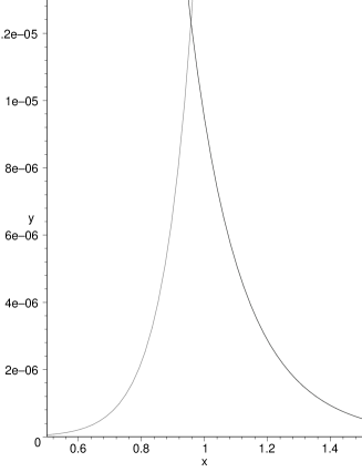
FIG. 4.: The inclusive gluon multiplicity $x^{4/5}\sigma(x)$ versus energy in units of the sphaleron mass $x=Q/M_{s}$.

FIG. 5.: The ratio (77) of prompt gluons emitted as a function of $-t/M_{S}^{2}$.

VI Conclusions

We have presented a semiclassical assessment of the inelastic cross section for multi-gluon production through instanton induced parton-parton scattering, using singular classical solutions to the Euclidean Yang-Mills equations. For energies $Q$ much above the sphaleron mass we have found an approximate but explicit solution which allowed us to obtain the field configuration at the turning (escape) time t=0. The approximate solution turns out to be just a rescaled Yang-Mills sphaleron solution [10]. We have solved the corresponding Yang-Mills equations describing its Minkowski explosion at later time, which is just a rescaled version of a Luscher-Schechter solution discussed in [10]. We have used the asymptotic form of the gauge field in physical gauge, to discuss the gluon number and spectrum.

Using an analytical continuation of the singular tails into Euclidean time, we have found that the same rescaling allows for the determination of the virtual in-gluon multiplicities both above and below the sphaleron (antisphaleron) point. Thus, the in-out multiplicities at the sphaleron and antisphaleron point, implies the in-out multiplicities away from this point for semiclassical parton-parton scattering. The scattering liberates about $1.1/\alpha_{s}(\rho)$ prompt gluons by sphaleron (antisphaleron) produced. We recall that all the calculations are semiclassical, assuming $\alpha_{s}(\rho)\ll 1$ or large produced multiplicities. The larger the longitudinal $Q$ transferred in the CM frame, the smaller the size of the escaping sphaleron or antisphaleron and vice versa. The semiclassical production through singular QCD solutions in the semi-hard regime, may even extend to the hard regime through smaller size sphalerons. However, in this case the cross section is small. On the other hand, for typical instantons in the instanton vacuum relevant to the ‘semi-hard’ scale and possibly to the QCD pomeron problem, this number turns out to be only about 3 gluons per cluster. In QCD there would be also quark production which we will discuss elsewhere.

This mechanism of coherent multi-gluon production is additional to perturbative BFKL ladders and/or virtual gluon materialization in the color-glass approach [17]. The difference between this mechanism and others is seen e.g. in the fact that the released semiclassical gluons form thin shells of strong coherent field, which carry topological features inherited from the topological tunneling. This difference is important for many applications, including the production of quarks as we discuss next.

Acknowledgments

This work was supported in parts by the US-DOE grant DE-FG-88ER40388. RJ was supported in part by KBN grants 2P03B01917 and 2P03B09622.

A LS solution

In this section we give a brief characterization of the LS gauge configuration. The reader is also referred to [16] for more details. For the Euclidean Witten ansatz

$$-eA^{a}_{0}= \frac{x_{a}}{r}A_{0}$$ (A1)

$$-eA^{a}_{i}= \varepsilon_{ian}\frac{x_{n}}{r^{2}}(1+\phi_{2})$$ (A3)

$$+\frac{x_{a}x_{i}}{r^{2}}A_{1}+\left(\delta_{ai}-\frac{x_{a}x_{i}}{r^{2}}\right)\frac{\phi_{1}}{r}$$

The coefficient functions for the LS solutions continued to Euclidean space are

$$A_{0} = -4q_{LS}\gamma^{2}rt$$ (A4)

$$A_{1} = -4q_{LS}\gamma^{2}\frac{1+r^{2}-t^{2}}{2}$$ (A5)

$$\phi_{1} = -4q_{LS}\gamma^{2}r\frac{1-r^{2}-t^{2}}{2}$$ (A6)

$$\phi_{2} = -4q_{LS}\gamma^{2}r^{2}-1$$ (A7)

$$\gamma^{2}=\frac{1}{(1-r^{2}-t^{2})^{2}+4r^{2}}$$ (A8)

and $q_{LS}$ is a function of $\mbox{arctanh}\left(\frac{2t}{1+r^{2}+t^{2}}\right)$.

In terms of these quantities the electric and magnetic fields are given by formula (7.27) in [16]. We perform the calculations for the sphaleron point which corresponds to

$$q_{LS}=-1+\frac{\sqrt{2}}{\cos\left(\sqrt{2}\mbox{arctanh}\left(\frac{2t}{1+r^{2}+t^{2}}\right)\right)}$$ (A9)

We rotate these formulas back to Minkowski space using $t\to it$. The solutions are again concentrated on the light cone. We perform then the limit $t\to\infty$ keeping $v=r-t$ fixed. The results for the ‘electric’ coefficients of formula (7.27) in [16] are

$$D_{0}\phi_{2}/r \longrightarrow \frac{v+2\mbox{sech}^{2}u(\sinh u-v)}{t(1+v^{2})^{2}}$$ (A10)

$$F_{01} \longrightarrow \frac{1}{t}\cdot 0$$ (A11)

$$D_{0}\phi_{1}/r \longrightarrow \frac{1-2\mbox{sech}^{2}u(v\sinh u+1)}{t(1+v^{2})^{2}}$$ (A12)

where $u\equiv\sqrt{2}\mbox{arctanh}(1/v)$. The ‘magnetic’ coefficients are

$$-D_{1}\phi_{1}/r \longrightarrow i\frac{1-2\mbox{sech}^{2}u(v\sinh u+1)}{t(1+v^{2})^{2}}$$ (A13)

$$(1-\phi_{1}^{2}-\phi_{2}^{2})/r^{2} \longrightarrow \frac{1}{t}\cdot 0$$ (A14)

$$D_{1}\phi_{2}/r \longrightarrow -i\frac{v+2\mbox{sech}^{2}u(\sinh u-v)}{t(1+v^{2})^{2}}$$ (A15)

For large times $t$, the electric and magnetic fields are equal

$${\vec{E}}^{2}(t,v)\sim{\vec{B}}^{2}(t,v)\sim\frac{2}{t^{2}}\,\frac{1}{(1+v^{2})^{3}}\,\,$$ (A16)

and sums up to $M_{S}$. The same result was obtained in [10].

The ‘antisphaleron’ follows from the sphaleron by substituting

$$A_{0} \longrightarrow -A_{0}$$ (A17)

$$A_{1} \longrightarrow -A_{1}$$ (A18)

$$\phi_{1} \longrightarrow -\phi_{1}$$ (A19)

$$\phi_{2} \longrightarrow \phi_{2}$$ (A20)

in the Witten ansatz above, and yields a solution of the YM equation of motion. The same transformation makes a switch between the instanton and antiinstanton in the Witten ansatz.

B $\mbox{\rm Im }S$ for LS Solution

In this appendix we will show that the imaginary part of the classical action along the deformed contour [15] does not depend on the energy of the LS solution. In other words, the instanton-antiinstanton suppression factor persits all the way to the sphaleron point in the deformed contour approach suggested in [15]. Indeed, for $\varepsilon<1/2$ the solution is given by the function

$$q=q_{-}\mbox{\rm sn}(q_{+}\phi+K,k)$$ (B1)

where we use the same notation as in [15]

$$q_{\pm}=\sqrt{1\pm\sqrt{2\varepsilon}}\quad\quad\quad\quad k^{2}=\frac{q_{-}^{2}}{q_{+}^{2}}$$ (B2)

and

$$\phi={\rm arccoth}\left(\frac{1+r^{2}+\tau^{2}}{2\tau}\right)$$ (B3)

The suppression factor is given by

$$\mbox{\rm Im }S=-\frac{24\pi^{2}}{g^{2}}\int_{0}^{\infty}dr\,\mbox{\rm Im }\sum_{nm}\mbox{\rm Res}\left\{\frac{\cos^{4}w}{r^{2}}{\cal E}\right\}$$ (B4)

where

$${\cal E}\equiv\frac{1}{2}\dot{q}^{2}+\frac{1}{2}(q^{2}-1)^{2}$$ (B5)

The residues are calculated at the poles of (B1) inside the contour. One can show that ${\cal E}$ is just equal to $(q^{2}-1)^{2}-\varepsilon$. We will now use the Laurent expansion of the elliptic sine

$$\mbox{\rm sn}(u)\sim\frac{\alpha}{u-u_{0}}+\beta(u-u_{0})$$ (B6)

Using the differential equation for $\mbox{\rm sn}(u)$ we obtain the relations $\alpha^{2}k^{2}=1$ and $\beta=\frac{\alpha}{6}(1+k^{2})$. We thus have to compute

$$\mbox{\rm Res}\left(\cos^{4}w{\cal E}\right)=\alpha^{4}k^{4}\mbox{\rm Res}\left(\frac{\cos^{4}w}{(\phi-\phi_{0})^{4}}\right)+$$ (B7)

$$(4\alpha^{3}\beta k^{2}q_{-}^{2}-2\alpha^{2}k^{2})\mbox{\rm Res}\left(\frac{\cos^{4}w}{(\phi-\phi_{0})^{2}}\right)$$ (B8)

The coefficients of the residues are energy independent and equal to $1$ and $-2/3$ respectively. Once we use

$$\cos^{2}w\equiv\frac{4r^{2}}{(1+r^{2})^{2}+2\tau^{2}(r^{2}-1)+\tau^{4}}$$ (B9)

and the $r$ dependence of the poles $\tau(r)=q+\sqrt{q^{2}-1-r^{2}}$ where $q$ is an $\varepsilon$ dependent constant, we obtain

$$\int_{0}^{\infty}\frac{dr}{r^{2}}\,\mbox{\rm Res}\left(\frac{\cos^{4}w}{(\phi-\phi_{0})^{4}}\right) = \frac{i}{3}\frac{1+q^{2}}{1-q^{2}}$$ (B10)

$$\int_{0}^{\infty}\frac{dr}{r^{2}}\,\mbox{\rm Res}\left(\frac{\cos^{4}w}{(\phi-\phi_{0})^{2}}\right) = i\frac{1}{1-q^{2}}$$ (B11)

Finally we get

$$\mbox{\rm Im }S=\frac{8\pi^{2}}{g^{2}}$$ (B12)

Note that the whole energy dependence through $\varepsilon$ has cancelled out.

C Stability under Perturbative Pair Production

Are the escaping Yang-Mills fields stable under pair production, at least perturbatively? In general, they include electric as well as magnetic fields: but the answer can still be given by assessing the gluon/quark pair emission rate in a general time dependent background to first order in $\alpha$. Let ${\cal T}(A)$ be the on-shell matrix element between a particle and an antiparticle in the external gauge field. Typically, the number of pairs per unit 4-volume is

$$\frac{dN_{\overline{q}q}}{d^{4}x}={\rm Tr}{\Big{<}}x|\,{\rm ln}\,\left({\bf 1}-{\cal T}(A)\,{\bf P}(+)\,{\overline{\cal T}}(A)\,{\bf P}(-)\right)|x{\Big{>}}$$ (C1)

where ${\bf P}(\pm)$ are the on-shell projectors on particles and antiparticles, and the trace is over color and spin. In the momentum representation

$${\bf P}(\pm)=2\pi\,(\hbox to0.0pt{/\hss}{P}+m_{F})\,\theta(\pm P_{0})\,\delta(P^{2}-m_{F}^{2})\,\,,$$ (C2)

for a flavor of mass $m_{F}$. Since the pair creation follows from large times (weak fields), we may approximate ${\cal T}(A)$ by its leading order

$${\cal T}(A)\approx ig\hbox to0.0pt{/\hss}{A}\,\,.$$ (C3)

Inserting (C3) into (C1), expanding the logarithm, integrating over all spacetime, and insisting on gauge invariance yield the pair rate

$$\frac{dN_{\overline{q}q}}{d^{4}q}= \frac{{\bf 4}\alpha}{12\,(2\pi)^{4}}\,\,\left(|{\bf E}_{i}^{a}(q)|^{2}-|{\bf B}_{i}^{a}(q)|^{2}\right)$$ (C5)

$$\times\theta(q^{2}-4m_{F}^{2})\,(1-4m_{F}^{2}/q^{2})^{1/2}(1+2m_{F}^{2}/q^{2})\,\,.$$

where $({\bf E}\,,{\bf B})$ are the Fourier transform of the chromo-electric and -magnetic fields in Minkowski space

$$({\bf E},{\bf B})\,(q)=\int d^{4}x\,e^{iq\cdot x}\,({\bf E},{\bf B})\,(x)\,\,.$$ (C7)

We have highlighted ${\bf 4}$ in (LABEL:45) to show

$${\bf 4}=\frac{1}{2}\times 2\times 2\times 2$$ (C8)

for $g/\sqrt{2}$ fundamental quark charge, 2 flavors, 2 spins and 2 particle-antiparticle respectively. Notice that the production in (LABEL:45) is time like, for which $q=(\omega,\vec{0})$ is an allowed frame. Such frames support zero magnetic fields, indicating that the pair production mechanism is electric in nature. It is of order $\alpha^{0}$ in the strong coupling constant. In deriving (C7) we have ignored the back-reaction of the quarks on the YM fields.

Since the $\overline{u}u$ and $\overline{d}d$ pairs are light, we may set $m_{F}\approx 0$ in (LABEL:45). The total number of light quark pairs emitted by the classical field is

$$N_{\overline{u}u+\overline{d}d}= \frac{\alpha}{3(2\pi)^{4}}\,\int d^{4}q\,\theta(q^{2})\,\left(|{\bf E}_{i}^{a}(q)|^{2}-|{\bf B}_{i}^{a}(q)|^{2}\right)\,\,.$$ (C9)

The present arguments can also be used to derive a similar expression for the number of gluon pairs emitted by the classical field in the weak field limit. For $N_{c}=3$, the gluons can be organized in 3 conjugate pairs, such as: $W^{+}W^{-}$, $K^{+}K^{-}$, $K^{0}\overline{K^{0}}$ by analogy with the charged octet mesons. Say we choose the external field to be $K^{0}$, then $K^{0}$ may decay into the two charged modes $W^{+}W^{-}$ and $K^{+}K^{-}$. Using the background field method, the result for the two gluon multiplicity is

$$N_{gg}= \frac{{\bf 3}\,\alpha}{12(2\pi)^{4}}\,\int d^{4}q\,\theta(q^{2})\,\left(|{\bf E}_{i}^{a}(q)|^{2}-|{\bf B}_{i}^{a}(q)|^{2}\right)\,\,,$$ (C11)

We have highlighted ${\bf 3}$,

$${\bf 3}=\frac{3}{4}\times 2\times 2$$ (C13)

for $g\sqrt{3}/2$ charge, 2 decay modes and 2 physical helicities respectively. Combining (LABEL:x46) with (LABEL:x47) we find that the light quark and gluon multiplicities are related

$$N_{\overline{u}u+\overline{d}d}=\frac{2N_{F}}{3}N_{gg}\,\,.$$ (C14)

Using the results of appendix B, we find

$$\int d^{4}q\,\theta(q^{2})\,\left(|{\bf E}_{i}^{a}(q)|^{2}-|{\bf B}_{i}^{a}(q)|^{2}\right)=0\,\,.$$ (C15)

The expanding sphaleron starts magnetic and remains magnetic-like throughout. It is stable under light-pairs quantum emission.

REFERENCES

- [1] A. Belavin, A. Polyakov, A. Shvarts and Y. Tyupkin, Phys. Lett. B59 (1975) 85.
- [2] G.t’Hooft Phys. Rev. D14 (1976) 3432; [Erratum-ibid. D 18 (1976) 2199].
- [3] T. Schafer and E. V. Shuryak, Rev. Mod. Phys. 70 (1998) 323.
- [4] A. Ringwald, Nucl. Phys. B330 (1990) 1; O. Espinosa, Nucl. Phys. B343 (1990) 310; V. Khoze, A. Ringwald, Phys. Lett. B259 (1991) 106.
- [5] V. Zakharov, Nucl. Phys. B353 (1991) 683; M. Maggiore and M. Shifman, Phys. Rev. D46 (1992) 3550.
- [6] D. Diakonov and V. Petrov, Phys. Rev. D50 (1994) 266.
- [7] A. Ringwald and F. Schrempp, Phys. Lett. B503 (2001) 331; F. Schrempp, hep-ph/0109032.
- [8] E. Shuryak and I. Zahed, Phys. Rev. D62 (2000) 085014; M. Nowak, E. Shuryak and I. Zahed, Phys. Rev. D64 (2001) 034008.
- [9] D. Kharzeev, Y. Kovchegov and E. Levin, Nucl. Phys. A690 (2001) 621.
- [10] D. Ostrovsky, G. Carter and E. Shuryak, hep-ph/0204224 Submitted to Phys.Rev.D.
- [11] S. Khlebnikov, Phys. Lett. B282 (1992) 459.
- [12] S. Khlebnikov, V. Rubakov and P. Tinyakov, Nucl. Phys. B350 (1991) 441.
- [13] M. Luscher, Phys. Lett. B70 (1977) 321; B. Schechter, Phys. Rev. D16 (1977) 3015.
- [14] M. Hellmund and J. Kripfganz B373 (1991) 749; J. Zadrozny, Phys. Lett. B284 (1992) 88; D. Diakonov and M. Polyakov, Phys. Rev. D49 (1994) 6864; J. Schaldach, P. Sieber, D. Diakonov and K. Goeke, hep-ph/9603224.
- [15] T. Gould and E. Poppitz, hep-ph/9305263; D. Son and P. Tinyakov, hep-ph/9309332.
- [16] A. Actor, Rev. Mod. Phys. 51 (1979) 461.
- [17] L. McLerran and R. Venugopalan, Phys. Rev. D49 (1994) 2233; 3352.