THE CHESHIRE CAT HADRONS REVISITED
Mannque Rho
Service de Physique Théorique, CEA/DSM/SPhT,
Unité de recherche associée au CNRS, CEA/Saclay
91191 Gif-sur-Yvette cédex, France
FOREWORD

In 1993, I gave a series of lectures “ELAF93” at the Latin American School of Physics at Mar del Plata, Argentina, on “Cheshire Cat Hadrons” which then appeared in hep-ph/9310300 and was published in Phys. Rep. 240 (1994) 1. In addition to a (shamefully) large number of trivial as well less trivial typographical errors and misprints, some of the concepts developed there and the arguments presented to support them turned out to be either incomplete or defective if not entirely wrong. Most of them have since been corrected and further clarified. I thought it to be fair to those who read the review to point out what’s not correct and what’s incomplete in the published version. More importantly, there have been significant novel developments in some of the materials covered at the time which are revived in an intriguing context in the current research activity in the physics of hadrons under extreme conditions. The purpose of this article is to correct the errors uncovered thus far in the original version and to supplement the revised version with a brief account of the modern understanding of the matters which were treated incorrectly or incompletely at the time. I will keep the original version, with however the erroneous results or statements pointed out in the footnotes and the relevant chapters preceded with short summaries of the novel developments and followed with the details of the selected issues in the appendices at the end of the chapters involved. To distinguish from the original ELAF93, the additions and corrections are put in italics.

INTRODUCTION

[Updating remark]

[The principal notion developed in this series of lectures “ELAF93,” Cheshire Cat Principle (CCP), touches on a variety of related concepts that are a lot more general than originally thought. Apart from the notion that physics should not depend upon the “confinement size” per se which was the principal theme of the ELAF93, it turns out now as I shall develop in this revised version that one can match the flavor symmetry – which is an “emergent” symmetry phrased in terms of Berry potentials – to a fundamental gauge symmetry, namely color symmetry of QCD. Amazingly, one can not only generate the symmetry bottom up as a hidden gauge symmetry that incorporates the observed vector particles as “hidden gauge bosons” but also obtain it top down from color gauge symmetry as a manifestation of spontaneous breaking of the color gauge symmetry. The modern development involves “color flavor locking” observed at superhigh density and conjectured at low densities, gluon-meson/quark-baryon dualities, the scaling of hadron properties in density and temperature – so-called “BR scaling” – related to Fermi-liquid fixed point quantities, the matching of effective field theories with QCD etc. Not all these concepts are well formulated and understood. Some are rather loose in conception but the challenge is to make the connections as firm as possible and test them against the future experiments to be performed at various laboratories in the world. I will discuss them at appropriate places with concrete examples.]

In this series of lectures, I would like to describe how far one can go in understanding hadronic properties, both elementary and many-body, at low energy based principally on generic features of the fundamental theory, QCD. For this I will use a specific simplified model, the chiral bag model, but the results should not crucially depend upon its characteristics. In fact, what matters is the generic consequence of symmetries considered, not the dynamical details of the model. If one wishes, once the generic structure is extracted, one can simply forget about the model without losing relevant physics.

This way of approaching hadron and nuclear physics is in line with the effective theory approach to other fields of physics. As emphasized since some time by Nambu [1], one generic effective theory, Ginzburg-Landau or Gell-Mann-Lévy Lagrangian, is able to capture the essence of the physics of superconductivity, ³He superfluidity, nuclear pairing, low-energy QCD and standard model with appropriately rescaled length parameters such as gap and condensate parameters. It is an intriguing fact of Nature that a sigma model so aptly describes the generic structure of all these interactions. Recently this point is given a more rigorous basis by Polchinski, Weinberg and others [2, 3] in terms of effective actions. Effective actions play an important role in two ways: One, when fundamental theory is not known above a certain energy scale as in the case of the standard model; two, when fundamental theory is known but the solution is unknown as in the case of QCD at low energy. In both cases, symmetries of the physical particles that one is trying to describe allow one to write the effective actions. In this lecture we are concerned with the latter.

The aim of this lecture is to show how much of low-energy properties of elementary hadrons and many-hadron systems can be understood with a set of effective degrees of freedom consistent with chiral symmetry of light quarks and heavy-quark symmetry of massive quarks. In doing this, I will resort to the Cheshire Cat philosophy [4]. Now while exact in two dimensions, the Cheshire cat can only be approximate in four dimensions. Clearly it would be meaningless to try to be too quantitative. Furthermore this cannot be a substitute for a real QCD calculation. But I feel that one can learn a lot here as one does in other areas of physics .

This lecture consists of three broad sections. In the first, I use the chiral bag model and the Cheshire Cat approach to “guess” an effective Lagrangian for hadrons. The notion of induced gauge fields as Berry potentials on the strong interaction sector is introduced. In the second, I apply a simple effective theory to describe the ground-state and excited-state properties of both light and heavy baryons. In the last, some properties of nuclei and nuclear matter are treated in terms of effective chiral Lagrangians motivated in the two preceding lectures.

The nature of this note is strongly influenced by my collaborations or discussions with many people, in particular with Gerry Brown, Andy Jackson, Kuniharu Kubodera, Hyun Kyu Lee, Dong-Pil Min, Holger Bech Nielsen, Maciej Nowak, Tae-Sun Park, Dan Olof Riska, Norberto Scoccola, Andreas Wirzba, Koichi Yamawaki and Ismail Zahed.

Part I “Guessing” an Effective Theory

1 The Cheshire Cat Principle (CCP)

[Updating remark]

[The Cheshire Cat Principle was conceived to explain how the low-energy properties of hadrons should not depend on the size of the space in which the quarks and gluons are confined. The key ingredient that enters here is the variety of quantum anomalies that induce certain quantum numbers such as baryon charge to leak out of the “confinement region” without upsetting the color gauge symmetry. The bottom line of the picture is that the degrees of freedom associated with the quarks and gluons can be transformed to and from the degrees of freedom associated with the hadrons. Since the confinement size is not a physical quantity, it is natural to elevate it to a gauge degree of freedom. This idea which was proposed in 1992 by Damgaard, Nielsen and Sollacher has not received much attention since then and there has been no further development along the given line. However what has been recently revived is the notion that the microscopic QCD degrees of freedom and the macroscopic hadronic degrees of freedom can be interchanged leading to the notion that there is “continuity” between quarks and baryons and also between gluons and mesons. This development will be discussed in a supplementary subsection in the last section.

What transpired in the context of the original Cheshire Cat Principle, in particular in connection with the structure of the nucleon, is summarized in a recent monograph [135] and the more recent development is given in a review article [136]. In a nutshell, there is no known case where the Cheshire Cat Principle is visibly violated although in four dimensions, the CCP cannot be quantitatively established except for topological quantities. Up to the time of [135], there was one case which was not in full conformity with the CCP and it had to do with the so-called “proton spin crisis.” Since then, this problem has found a simple resolution in terms of the ABJ anomaly [136]. This will be discussed in an appendix below.]

1.1 Toy Model in (1+1) Dimensions

In two dimensions the Cheshire Cat principle (CCP in short from now on) can be formulated exactly. Let us discuss it to have a general idea involved. Later we will make a leap to reality in four dimensions by making a guess. We shall use for definiteness the chiral bag picture[7]. The result is generic and should not sensitively depend upon details of the models. Thus other models of similar structure containing the same symmetries could be equally used. We will leave the construction to the aficionados of their own favorite models.

In the spirit of a chiral bag, consider a massless free single-flavored fermion $\psi$ confined in a region (say, inside) of “volume” $V$ coupled on the surface $\partial V$ to a massless free boson $\phi$ living in a region of “volume” $\tilde{V}$ (say, outside). Of course in one-space dimension, the “volume” is just a segment of a line but we will use this symbol in analogy to higher dimensions. We will assume that the action is invariant under global chiral rotations and parity. Interactions invariant under these symmetries can be introduced without changing the physics, so the simple system that we consider captures all the essential points of the construction. The action contains three terms

$$S=S_{V}+S_{\tilde{V}}+S_{\partial V}$$ (I.1)

where

$$S_{V} = \int_{V}d^{2}x\bar{\psi}i\gamma^{\mu}\partial_{\mu}\psi+\cdots,$$ (I.2)

$$S_{\tilde{V}} = \int_{\tilde{V}}d^{2}x\frac{1}{2}(\partial_{\mu}\phi)^{2}+\cdots$$ (I.3)

and $S_{\partial V}$ is the boundary term which we will specify shortly. Here the ellipsis stands for other terms such as interactions, fermion masses etc. consistent with the assumed symmetries of the system on which we will comment later. For instance, there can be a coupling to a $U(1)$ gauge field in (I.2) and a boson mass term in (I.3) as would be needed in Schwinger model. Without loss of generality, we will simply ignore what is in the ellipsis unless we absolutely need it. Now the boundary term is essential in making the connection between the two regions. Its structure depends upon the physics ingredients we choose to incorporate. We will assume that chiral symmetry holds on the boundary even if it is, as in Nature, broken both inside and outside by fermion mass terms. As long as the symmetry breaking is gentle, this should be a good approximation since the surface term is a $\delta$ function. We should also assume that the boundary term does not break the discrete symmetries ${\cal P}$, ${\cal C}$ and ${\cal T}$. Finally we demand that it give no decoupled boundary conditions, that is to say, boundary conditions that involve only $\psi$ or $\phi$ fields. These three conditions are sufficient in (1+1) dimensions to give a unique term[8]

$$S_{\partial V}=\int_{\partial V}d\Sigma^{\mu}\left\{\frac{1}{2}n_{\mu}\bar{\psi}e^{i\gamma_{5}\phi/f}\psi\right\}$$ (I.4)

with the $\phi$ “decay constant” $f=1/\sqrt{4\pi}$ where $d\Sigma^{\mu}$ is an area element with $n^{\mu}$ the normal vector, i.e, $n^{2}=-1$ and picked outward-normal. As we will mention later, we cannot establish the same unique relation in (3+1) dimensions but we will continue using this simple structure even when there is no rigorous justification in higher dimensions.

At classical level, the action (I.1) gives rise to the bag “confinement,” namely that inside the bag the fermion (which we shall call “quark” from now on) obeys

$$i\gamma^{\mu}\partial_{\mu}\psi=0$$ (I.5)

while the boson (which we will call “pion”) satisfies

$$\partial^{2}\phi=0$$ (I.6)

subject to the boundary conditions on $\partial V$

$$in^{\mu}\gamma_{\mu}\psi = -e^{i\gamma_{5}\phi/f}\psi,$$ (I.7)

$$n^{\mu}\partial_{\mu}\phi = f^{-1}\bar{\psi}(\frac{1}{2}n^{\mu}\gamma_{\mu}\gamma_{5})\psi.$$ (I.8)

Equation (I.7) is the familiar “MIT confinement condition” which is simply a statement of the classical conservation of the vector current $\partial_{\mu}j^{\mu}=0$ or $\bar{\psi}\frac{1}{2}n^{\mu}\gamma_{\mu}\psi=0$ at the surface while Eq. (I.8) is just the statement of the conserved axial vector current $\partial_{\mu}j_{5}^{\mu}=0$ (ignoring the possible explicit mass of the quark and the pion at the surface). The crucial point of our argument is that these classical observations are invalidated by quantum mechanical effects. In particular while the axial current continues to be conserved, the vector current fails to do so due to quantum anomaly.

There are several ways of seeing that something is amiss with the classical conservation law, with slightly different interpretations. The easiest way is as follows. For definiteness, let us imagine that the quark is “confined” in the space $-\infty\leq r\leq R$ with a boundary at $r=R$. Now the vector current $j_{\mu}=\bar{\psi}\gamma_{\mu}\psi$ is conserved inside the “bag”

$$\partial^{\mu}j_{\mu}=0,\ \ \ \ \ r<R.$$ (I.9)

If one integrates this from $-\infty$ to $R$ in $r$, one gets the time-rate change of the fermion (i.e, quark) charge

$$\dot{Q}\equiv\frac{d}{dt}Q=2\int_{-\infty}^{R}dr\partial_{0}j_{0}=2\int_{-\infty}^{R}dr\partial_{1}j_{1}=2j_{1}(R)$$ (I.10)

which is just

$$\bar{\psi}n^{\mu}\gamma_{\mu}\psi,\ \ \ \ r=R.$$ (I.11)

This vanishes classically as we mentioned above. But this is not correct quantum mechanically because it is not well-defined locally in time. In other words, $\psi^{\dagger}(t)\psi(t+\epsilon)$ goes like $\epsilon^{-1}$ and so is singular as $\epsilon\rightarrow 0$. To circumvent this difficulty which is related to vacuum fluctuation, we regulate the bilinear product by point-splitting in time

$$j_{1}(t)=\bar{\psi}(t)\frac{1}{2}\gamma_{1}\psi(t+\epsilon),\ \ \ \ \ \epsilon\rightarrow 0.$$ (I.12)

Now using the boundary condition

$$i\gamma_{1}\psi(t+\epsilon) = e^{i\gamma_{5}\phi(t+\epsilon)/f}\psi(t+\epsilon)$$ (I.13)

$$\approx e^{i\gamma_{5}\phi(t)/f}[1+i\epsilon\gamma_{5}\dot{\phi}(t)/f]e^{\frac{1}{2}[\phi(t),\phi(t+\epsilon)]}\psi(t+\epsilon),\ \ \ \ r=R$$

and the commutation relation

$$[\phi(t),\phi(t+\epsilon)]=i\ {\rm sign}\ \epsilon,$$ (I.14)

we obtain

$$j_{1}(t)=-\frac{i}{4f}\epsilon\dot{\phi}(t)\psi^{\dagger}(t)\psi(t+\epsilon)=\frac{1}{4\pi f}\dot{\phi}(t)+O(\epsilon),\ \ \ \ r=R$$ (I.15)

where we have used $\psi^{\dagger}(t)\psi(t+\epsilon)=\frac{i}{\pi\epsilon}+[{\rm regular}]$. Thus quarks can flow out or in if the pion field varies in time. But by fiat, we declared that there be no quarks outside, so the question is what happens to the quarks when they leak out? They cannot simply disappear into nowhere if we impose that the fermion (quark) number is conserved. To understand what happens, rewrite (I.15) using the surface tangent

$$t^{\mu}=\epsilon^{\mu\nu}n_{\nu}.$$ (I.16)

We have

$$t\cdot\partial\phi=\frac{1}{2f}\bar{\psi}n\cdot\gamma\psi=\frac{1}{2f}\bar{\psi}t\cdot\gamma\gamma_{5}\psi,\ \ \ \ r=R$$ (I.17)

where we have used the relation $\bar{\psi}\gamma_{\mu}\gamma_{5}\psi=\epsilon_{\mu\nu}\bar{\psi}\gamma^{\nu}\psi$ valid in two dimensions. Equation (I.17) together with (I.8) is nothing but the bosonization relation

$$\partial_{\mu}\phi=f^{-1}\bar{\psi}(\frac{1}{2}\gamma_{\mu}\gamma_{5})\psi$$ (I.18)

at the point $r=R$ and time $t$. As is well known, this is a striking feature of (1+1) dimensional fields that makes one-to-one correspondence between fermions and bosons[9]. In fact, one can even write the fermion field in terms of the boson field as

$$\psi(x)={\rm exp}\left\{-\frac{i}{2f}\int_{x_{0}}^{x}d\xi[\pi(\xi)+\gamma_{5}\phi^{\prime}(\xi)]\right\}\psi(x_{0})$$ (I.19)

where $\pi(\xi)$ is the conjugate field to $\phi(\xi)$ and $\phi^{\prime}(\xi)=\frac{d}{d\xi}\phi(\xi)$.

Equation (I.10) with (I.15) is the vector anomaly, i.e, quantum anomaly in the vector current: The vector current is not conserved due to quantum effects. What it says is that the vector charge which in this case is equivalent to the fermion (quark) number inside the bag is not conserved. Physically what happens is that the amount of fermion number $\Delta Q$ corresponding to $\Delta t\dot{\phi}/\pi f$ is pushed into the Dirac sea at the bag boundary and so is lost from inside and gets accumulated at the pion side of the bag wall. This accumulated baryon charge must be carried by something residing in the meson sector. Since there is nothing but “pions” outside, it must be be the pion field that carries the leaked charge. This means that the pion field supports a soliton. This is rather simple to verify in (1+1) dimensions using arguments given in the work of Coleman and Mandelstam [9], referred to above. This can also be shown to be the case in (3+1) dimensions. In the present model, we find that one unit of fermion charge $Q=1$ is partitioned as

$$Q = 1=Q_{V}+Q_{\tilde{V}},$$ (I.20)

$$Q_{\tilde{V}} = \theta/\pi,$$

$$Q_{V} = 1-\theta/\pi$$

with

$$\theta=\phi(R)/f.$$ (I.21)

We thus learn that the quark charge is partitioned into the bag and outside of the bag, without however any dependence of the total on the size or location of the bag boundary. In (1+1)-dimensional case, one can calculate other physical quantities such as the energy, response functions and more generally, partition functions and show that the physics does not depend upon the presence of the bag[10]. We could work with quarks alone, or pions alone or any mixture of the two. If one works with the quarks alone, we have to do a proper quantum treatment to obtain something which one can obtain in mean-field order with the pions alone. In some situations, the hybrid description is more economical than the pure ones. The complete independence of the physics on the bag – size or location– is called the “Cheshire Cat Principle” (CCP) with the corresponding mechanism referred to as “Cheshire Cat Mechanism” (CCM). Of course the CCP holds exactly in (1+1) dimensions because of the exact bosonization rule. There is no exact CCP in higher dimensions since fermion theories cannot be bosonized exactly in higher dimensions but we will see later that a fairly strong case of CCP can be made for (3+1) dimensional models. Topological quantities like the fermion (quark or baryon) charge satisfy an exact CCP in (3+1) dimensions while nontopological observables such as masses, static properties and also some nonstatic properties satisfy it approximately but rather well.

1.1.1 “Color” anomaly

So far we have been treating the quark as “colorless”, in other words, in the absence of a gauge field. Let us consider that the quark carries a $U(1)$ charge $e$, coupling to a $U(1)$ gauge field $A^{\mu}$. We will still continue working with a single-flavored quark, treating the multi-flavored case later. Then inside the bag, we have essentially the Schwinger model, namely, (1+1)-dimensional QED[11]. It is well established that the charge is confined in the Schwinger model, so there are no charged particles in the spectrum. If now our “leaking” quark carries the color (electric) charge, this will at first sight pose a problem since the anomaly obtained above says that there will be a leakage of the charge by the rate

$$\dot{Q^{c}}=\frac{e}{2\pi}\dot{\phi}/f.$$ (I.22)

This means that the charge accumulated on the surface will be

$$\Delta Q^{c}=\frac{e}{2\pi}\phi(t,R)/f.$$ (I.23)

Unless this is compensated, we will have a violation of charge conservation, or breaking of gauge invariance. This is unacceptable. Therefore we are invited to introduce a boundary condition that compensates the induced charge, i.e, by adding a boundary term

$$\delta S_{\partial V}=-\int_{\partial V}d\Sigma\frac{e}{2\pi}\epsilon^{\mu\nu}n_{\nu}A_{\mu}\frac{\phi}{f}$$ (I.24)

with $n^{\mu}=g^{\mu\nu}n_{\nu}$. The action is now of the form [12]

$$S=S_{V}+S_{\tilde{V}}+S_{\partial V}$$ (I.25)

with

$$S_{V} = \int_{V}d^{2}x\left\{\bar{\psi}(x)\left[i\partial_{\mu}-eA_{\mu}\right]\gamma^{\mu}\psi(x)-\frac{1}{4}F_{\mu\nu}F^{\mu\nu}\right\},$$ (I.26)

$$S_{\tilde{V}} = \int_{\tilde{V}}d^{2}x\left\{\frac{1}{2}(\partial_{\mu}\phi(x))^{2}-\frac{1}{2}m_{\phi}^{2}\phi(x)^{2}\right\},$$ (I.27)

$$S_{\partial V} = \int_{\partial V}d\Sigma\left\{\frac{1}{2}\bar{\psi}e^{i\gamma^{5}\phi/f}\psi-\frac{e}{2\pi}\epsilon^{\mu\nu}n_{\mu}A_{\nu}\frac{\phi}{f}\right\}.$$ (I.28)

We have included the mass of the $\phi$ field, the reason of which will become clear shortly.

In this example, we are having the “pion” field (more precisely the soliton component of it) carry the color charge. In general, though, the field that carries the color could be different from the field that carries the soliton. In fact, in (3+1) dimensions, it is the $\eta^{\prime}$ field that will be coupled to the gauge field (although $\eta^{\prime}$ is colorless) while it is the pion field that supports a soliton. But in (1+1) dimensions, the soliton is lodged in the $U(1)$ flavor sector (whereas in (3+1) dimensions, it is in $SU(n_{f})$ with $n_{f}\geq 2$). For simplicity, we will continue our discussion with this Lagrangian.

We now illustrate how one can calculate the mass of the $\phi$ field using the action (I.25) and the CCM. This exercise will help understand a similar calculation of the mass of the $\eta^{\prime}$ in (3+1) dimensions. The additional ingredient needed for this exercise is the $U_{A}(1)$ (Adler-Bell-Jackiw) anomaly [13] which in (3+1) dimensions reads

$$\partial_{\mu}j_{5}^{\mu}=-\frac{e^{2}}{32\pi^{2}}\epsilon_{\mu\nu\rho\sigma}F^{\mu\nu}F^{\rho\sigma}$$ (I.29)

and in (1+1) dimensions takes the form

$$\partial_{\mu}j_{5}^{\mu}=-\frac{e}{4\pi}\epsilon_{\mu\nu}F^{\mu\nu}=-\frac{1}{2\pi}eE.$$ (I.30)

Instead of the configuration with the quarks confined in $r<R$, consider a small bag “inserted” into the static field configuration of the scalar field $\phi$ which we will now call $\eta^{\prime}$ in anticipation of the (3+1)-dimensional case we will consider later. Let the bag be put in $-\frac{R}{2}\leq r\leq\frac{R}{2}$. The CCP states that the physics should not depend on the size $R$, hence we can take it to be as small as we wish. If it is small, then the charge accumulated at the two boundaries will be $\pm\frac{e}{2\pi}\phi/f$. This means that the electric field generated inside the bag is

$$E=F_{01}=\frac{e}{2\pi}(\phi/f).$$ (I.31)

Therefore from the $U_{A}(1)$ anomaly (I.30), the axial charge created or destroyed (depending on the sign of the scalar field) in the static bag is

$$2\int_{V}dr\partial_{\mu}j_{5}^{\mu}=2(-j_{1}^{5}|_{\frac{R}{2}}+j_{1}^{5}|_{-\frac{R}{2}})=-\frac{e^{2}}{2\pi^{2}}(\phi/f)R.$$ (I.32)

From the bosonization condition (I.18), we have

$$2f\left(\partial_{1}\phi|_{\frac{R}{2}}-\partial_{1}\phi|_{-\frac{R}{2}}\right)=\frac{e^{2}}{2\pi^{2}}(\phi/f)R.$$ (I.33)

Now taking $R$ to be infinitesimal by the CCP, we have, on cancelling $R$ from both sides,

$$\partial^{2}\phi-\frac{e^{2}}{4\pi^{2}f^{2}}\phi=0$$ (I.34)

which then gives the mass, with $f^{-2}=4\pi$,

$$m_{\phi}^{2}=\frac{e^{2}}{\pi},$$ (I.35)

the well-known scalar mass in the Schwinger model which can also be obtained by bosonizing the $(QED)_{2}$. A completely parallel reasoning will be used later to calculate the $\eta^{\prime}$ mass in (3+1) dimensions.

1.1.2 The Wess-Zumino-Witten term

Let us consider the case of more than one flavor. For simplicity, we take two flavors. We shall see later that in (3+1) dimensions, we have an extra topological term called Wess-Zumino-Witten term (WZW term in short, alternatively referred to as Wess-Zumino term) if we have more than two flavors. In (1+1) dimensions, such an extra term arises already for two flavors[14]. The relevant flavor symmetry is then $U(2)\times U(2)$. The $U_{V}(1)$ symmetry associated with the fermion number does not concern us, so we may drop it, leaving the symmetry $U_{A}(1)\times SU(2)\times SU(2)$. The scalar field discussed above corresponds to the $U_{A}(1)$ field, so we will not consider it anymore and instead focus on scalars living in $SU(2)_{V}$ to which $SU(2)\times SU(2)$ breaks down . The scalars will be called $\pi^{a}$ with $a=1,2,3$. As stated before, the soliton lives in the $U(1)$ sector, so the $SU(2)$ scalars have nothing to do with the “baryon” structure but its nonabelian nature brings in an extra ingredient associated with the Wess-Zumino-Witten term which we will now show emerges from the boundary condition. Let the scalar multiplets be summarized in the form

$$U=e^{i\vec{\tau}\cdot\vec{\pi}/f}$$ (I.36)

with $f=1/\sqrt{4\pi}$.

As before the action consists of three terms

$$S=S_{V}+S_{\tilde{V}}+S_{\partial V}.$$ (I.37)

The bag action is given as before by

$$S_{V} = \int_{V}d^{2}x\bar{\psi}i\gamma^{\mu}\partial_{\mu}\psi+\cdots,$$ (I.38)

where the fermion field is a doublet $\psi^{T}=(\psi_{1},\psi_{2})$. A straightforward generalization of the abelian boundary condition consistent with chiral invariance suggests the boundary term of the form

$$S_{\partial V}=\int_{\partial V}d\Sigma^{\mu}\left\{\frac{1}{2}n_{\mu}\bar{\psi}U^{\gamma_{5}}\psi\right\}$$ (I.39)

with

$$U^{\gamma_{5}}=e^{i\gamma_{5}\vec{\tau}\cdot\vec{\pi}/f}.$$ (I.40)

As is very well-known by now, the meson sector contains an extra term, the WZW term, which plays an important role in multi-flavor systems even for noninteracting bosons. This will be derived below using the Cheshire Cat mechanism. (For a standard derivation, see [14]). The outside (meson sector) contribution to the action takes the form

$$S_{\tilde{V}}=\int_{\tilde{V}}d^{2}x\frac{f^{2}}{4}{\mbox{Tr}}(\partial_{\mu}U\partial^{\mu}U^{\dagger})+\cdots+S_{WZW}.$$ (I.41)

As seen, the main new ingredient in this action is the presence of the extra term $S_{WZW}$ in the boson sector. This is the WZW term which in the (1+1)-dimensional system we are interested in takes the form

$$S^{\tilde{V}}_{WZW}=\frac{2\pi n}{24\pi^{2}}\int_{\tilde{V}\times[0,1]}d^{3}x\epsilon^{ijk}\,{\mbox{Tr}}(L_{i}L_{j}L_{k})$$ (I.42)

with an integer $n$ corresponding to the number of “colors”, where $L_{\mu}=g^{\dagger}\partial_{\mu}g$ with $g$ “homotopically” extended as $g(s=0,x)=1$, $g(s=1,x)=U(x)$. The action (I.42) is defined in the partial space $\tilde{V}$. As we will see later, the WZW term plays a crucial role in the skyrmion physics in (3+1) dimensions, so the question we wish to address here is: How does the Cheshire Cat manifest itself for the WZW term? To answer this question, we imagine shrinking the bag to a point and ask what remains from what corresponds to the WZW term coming from the space $V$ in which quarks live. The obvious answer would be that the bag gives rise to the portion of the WZW term complement to (I.42) so as to yield the total defined in the full space. This is of course the right answer but it is not at all obvious that the chiral bag theory as formulated does this properly. For instance, consider the variation of the action of the meson sector (I.42)

$$\delta S^{\tilde{V}}_{WZW} = 3\frac{n}{12\pi}\int_{\tilde{V}}d^{2}x\epsilon^{\mu\nu}{\mbox{Tr}}((g^{\dagger}\delta g)L_{\mu}L_{\nu})$$ (I.43)

$$+ 3\frac{n}{12\pi}\int_{0}^{1}ds\int_{\partial{\tilde{V}}}d\Sigma_{\mu}\epsilon^{\mu\nu\alpha}{\mbox{Tr}}((g^{\dagger}\delta g)L_{\nu}L_{\alpha}).$$

The second term depends on both the homotopy extension and the surface. By the CCP, such a term is unphysical and must be cancelled by a complementary contribution from the bag. Thus the consistency of the model requires that the cancellation occur through the boundary condition. We will now show this is exactly what one obtains within the model so defined [15].

Consider the action for the quark bag with the quark satisfying the Dirac equation

$$i\not\!{\partial}\psi=0$$ (I.44)

subject to the boundary condition

$$(e^{i\theta(\beta,t)\gamma_{5}}-\not\!{n})\psi(\beta,t)=0.$$ (I.45)

where the bag wall is put at $x=\beta$ and $\theta\equiv\vec{\tau}\cdot\vec{\pi}/f$. We will use the Weyl representation for the $\gamma$ matrices as before. We will move the bag wall such that the bag will shrink to zero radius. The general solution for (I.44) with (I.45) is

$$\psi(x,t)={\rm exp}\left\{-i[\frac{1}{2}(1+\gamma_{5})\theta_{-}+\frac{1}{2}(1-\gamma_{5})\theta_{+}]\right\}\psi_{0}(x,t)$$ (I.46)

where $\theta_{\pm}=\theta(x\pm t)$ and $\psi_{0}$ is the solution for $\theta=0$ (for the MIT bag). The boundary condition is satisfied if

$$\theta_{-}(\beta,t)-\theta_{+}(\beta,t)=\theta(\beta,t).$$ (I.47)

Since we are dealing with a time-dependent boundary condition , it is more convenient to use the path-integral method instead of a canonical formalism. Let $\not\!{\partial}_{\theta}$ denote the Euclidean Dirac operator associated with the boundary condition (I.45). Then integrating the quark field in the bag action, we have

$$e^{-S_{F}}={\rm det}\left(\not\!{\partial}_{\theta}/\not\!{\partial}_{0}\right)$$ (I.48)

or

$$S_{F}=-{\rm tr}\ {\rm ln}(\not\!{\partial}_{\theta}\not\!{\partial}_{0}^{-1})=-\int_{0}^{1}ds\,{\rm tr}(\partial_{s}\not\!{\partial}_{\theta}\not\!{\partial}_{\theta}^{-1})$$ (I.49)

where we denote by $S_{F}$ the effective Euclidean action for the bag. On the right-hand side of Eq.(I.49), $\theta$ is homotopically extended as $\theta(x,t)\rightarrow\theta(x,t,s)$ such that $\theta(x,t,s=1)=\theta(x,t)$ and $\theta(x,t,s=0)=0$. The trace tr goes over the “color”, the space-time, $\gamma$ matrices and the flavor ($\tau$) matrices. Since the $\theta$ dependence appears only in the boundary condition, we can use the latter to rewrite

$$S_{F}=-\int_{0}^{1}ds\,{\rm tr}\ \left(\Delta_{B}\partial_{s}[e^{i\theta\gamma_{5}}-\not\!{n}]\not\!{\partial}_{\theta}^{-1}\right)$$ (I.50)

where $\Delta_{B}$ is the surface delta function. This expression has a meaning only when it is suitably regularized. We use the point-splitting regularization

$$S_{F}=-\lim_{\epsilon\rightarrow 0_{+}}\int_{V\times[0,1]}dsd^{2}x\Delta_{B}{\rm tr}\ (\partial_{s}e^{i\gamma_{5}\theta}G_{\theta}(x,t+\epsilon;x,t-\epsilon))$$ (I.51)

with $G$ the Dirac propagator inside the chiral bag which can be written explicitly using the time-dependent solution (I.46)

$$G_{\theta}(x,t;x^{\prime},t^{\prime}) = \left(\begin{array}[]{cc}e^{-i\theta_{-}(x-t)}&0\\ 0&e^{-i\theta_{+}(x+t)}\end{array}\right)$$ (I.57)

$$G_{0}(x,t;x^{\prime},t^{\prime})\left(\begin{array}[]{cc}e^{i\theta_{+}(x^{\prime}+t^{\prime})}&0\\ 0&e^{i\theta_{-}(x^{\prime}-t^{\prime})}\end{array}\right)$$

where $G_{0}$ is the bagged-quark MIT propagator which has been computed by multiple-reflection method [17]

$$\lim_{x,x^{\prime}\rightarrow\beta}G_{0}(x,t+\epsilon;x^{\prime},t-\epsilon)=\frac{1}{4}(1+\gamma_{\beta}^{1})(\gamma^{0}/4\pi\epsilon)(3-\gamma_{\beta}^{1})+O(1)$$ (I.58)

with $\gamma_{\beta}^{1}=\gamma^{1}\cdot n_{\beta}$ and $n_{\beta}=n_{\pm}=\pm 1$. The WZW term arises from the imaginary part of the action, so calculating ${\rm Im}\ S_{F}$ to leading order in the derivative expansion, we get

$${\rm Im}\,S_{F}=i\frac{2\pi n}{24\pi^{2}}\int_{0}^{1}ds\int_{V}dxdt{\mbox{Tr}}\,(\partial_{s}\theta\partial_{t}\theta\partial_{x}\theta)+\cdots$$ (I.59)

where the trace Tr now runs only over the flavor indices and the ellipsis stands for higher derivative terms. Invoking chiral symmetry and going to the Minkowski space, we finally obtain

$$S_{WZW}^{V}=-i\frac{2\pi n}{24\pi^{2}}\int_{V\times[0,1]}d^{3}x\epsilon^{\mu\nu\alpha}{\mbox{Tr}}\,(L_{\mu}L_{\nu}L_{\alpha})$$ (I.60)

which is exactly the complement to the outside contribution (I.42). Notice that there is no surface-dependent term whose presence would have signaled the breakdown of the CCP.

So far our discussion has been a bit non-rigorous. A lot more rigorous derivation was given by Falomir, M.A. Muschietti and E.M. Santangelo [15] who computed the path integral

$$Z=\int{\cal D}\bar{\psi}{\cal D}\psi e^{-S_{E}}$$ (I.61)

where

$$S_{E}=\int_{V}d^{2}x\bar{\psi}e^{\gamma_{5}\theta}i\not\!{\partial}e^{\gamma_{5}\theta}\psi+\frac{1}{2}\int_{\partial V}d^{1}x\bar{\psi}(1+i\not\!{n})\psi.$$ (I.62)

A careful analysis showed indeed that there is no surface term in the effective action, corroborating the above derivation: the model is fully consistent with the CCP. Note that in (I.62), the field $\theta$ is defined in the interior of the volume $V$ whereas in the above consideration all the action occurred on the surface. The physics is equivalent, however, since our argument was based on “shrinking” the bag whereas in the formulation of these authors, the quarks are being plainly integrated out from the bag. (The real part of the effective action gives $S_{V}=\frac{f^{2}}{4}\int_{V}d^{2}x{\mbox{Tr}}\ (\partial_{\mu}U\partial^{\mu}U^{\dagger})+{\rm higher\ derivative\ terms}$, just to complement the meson sector.)

To summarize the point in case the readers did not find the above discussion illuminating, the Cheshire Cat argument provides a “derivation” of the WZW term in (1+1) dimensions. This is certainly not a very elegant derivation but ties the anomaly issue naturally with non-anomalous phenomena within the model. The same argument holds for (3+1) dimensions as shown by Chen et al. [15].

1.1.3 A bit more mathematics of the Wess-Zumino-Witten term

Here we give a slightly more rigorous explanation [18] of the WZW term we have derived. The argument can be easily extended to higher dimensions but the situation in (1+1) dimensions is vastly simpler.

Consider a field $g$ valued in the group $SU(N)$ with $N\geq 2$ (in the case of two dimensions) which we can represent by $N\times N$ unitary matrices with unit determinant. The configuration space $Q$ is given by fields in one spatial dimension. If we impose the boundary condition that $g\rightarrow 1$ at $x=\pm\infty$, so that at a fixed time, the space is a circle $S^{1}$, then $Q$ is just the set of maps

$$Q:S^{1} \rightarrow SU(N)$$

$$x^{1} \rightarrow g(x^{1}).$$ (I.63)

We will consider the WZW term in the full space $\Omega=V\cup\tilde{V}$. Now let $D$ be a disc in $Q$ parameterized by $x^{0}$ corresponding to time and an $s$ with $0\leq s\leq 1$ such that the boundary $D$ is just the space-time $\Omega$ (we are implicitly understanding that time is included therein). The field is then $g(x^{0},x^{1},s)$ chosen so that $g(x^{0},x^{1},0)=1$ and $g(x^{0},x^{1}.1)=g(x^{1})=U$. Then the WZW term in Euclidean space is

$$S_{WZW}=\frac{2\pi n}{24\pi^{2}}\int_{D[\partial D=\Omega\times[0,1]]}\epsilon_{ijk}\ {\mbox{Tr}}(g^{\dagger}\partial_{i}gg^{\dagger}\partial_{j}gg^{\dagger}\partial_{k}g).$$ (I.64)

This action has the properties that the quantity $n$ is quantized to an integer value and that the action is invariant under the infinitesimal variation in the interior of the disc $D$. One can see the latter in various ways. One way is to note that $S_{WZW}/(2\pi n)$ is just the charge of the winding number current

$$J_{\mu}=\frac{1}{24\pi^{2}}\epsilon_{\mu\nu\alpha\beta}{\mbox{Tr}}[g^{\dagger}\partial^{\nu}gg^{\dagger}\partial^{\alpha}gg^{\dagger}\partial^{\beta}g],$$ (I.65)

namely

$$S_{WZW}/(2\pi n)=\int d^{3}xJ_{0}(x)$$ (I.66)

which is just the conserved winding number. Another way of seeing this is to note that $S_{WZW}$ is just an integral of a closed three form. Now to show that $n$ is quantized, it suffices to notice that $D\cup\bar{D}=S^{2}\times S^{1}$ (where $\bar{D}$ is the disc complement to $D$) and that

$$\frac{2\pi n}{24\pi^{2}}\int_{S^{2}\times S^{1}}\ {\mbox{Tr}}[g^{\dagger}dg]^{3}=2\pi\times{\rm integer}.$$ (I.67)

This proves the assertion. Similar quantization of the coefficient of the WZW term in four dimensions will turn out to be crucial for skyrmion physics later.

1.2 Going to (3+1) Dimensions

Since we cannot bosonize completely even a free Dirac theory in four dimensions (not to mention highly nonlinear QCD), we will essentially follow step-by-step the (1+1)-dimensional reasoning and construct in complete parallel a simple, yet hopefully sufficiently realistic chiral bag model which will then be partially bosonized. The roles of CCP and bosonization will then be reversed here: We will invoke CCP in bosonizing the chiral bag. Here again the boundary conditions play a key role. Ultimately we will motivate a modelling of QCD at low energies in terms of effective chiral Lagrangian theory which we will use to describe low-energy hadronic/nuclear processes.

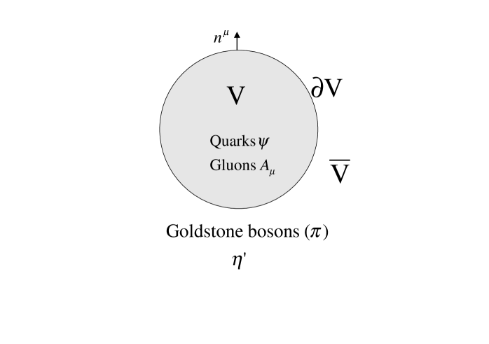
Figure 1: A spherical chiral bag for “deriving” a four-dimensional Cheshire Cat model. $\psi$ represents the doublet quark field of u and d quarks for $SU(2)$ flavor or the triplet of u, d and s for $SU(3)$ flavor and $\pi$ the triplet $\pi^{+},\pi^{-},\pi^{0}$ for $SU(2)$ and the octet pseudoscalars $\pi$, $K$, $\bar{K}$ and $\eta$ for $SU(3)$. The axial singlet meson $\eta^{\prime}$ figures in axial anomaly.

1.2.1 The model with $U_{A}(1)$ anomaly

For generality, we consider the flavor group $SU(3)\times SU(3)\times U_{A}(1)$ appropriate to up, down and strange quark systems. The chiral symmetry $SU(3)\times SU(3)$ is spontaneously broken down to $SU(3)$, with the octet Goldstone bosons denoted by $\pi=\frac{\lambda^{a}}{2}\pi^{a}$ with $\lambda$ the Gell-Mann matrices and the $U_{A}(1)$ symmetry is broken by anomaly, with the associated massive scalar denoted by $\eta^{\prime}$. Vector mesons can be suitably introduced through hidden gauge symmetry (HGS) but we will not use them here for simplicity. We do not yet have a fully satisfactory theory of Cheshire Cat mechanism in the presence of vector-meson degrees of freedom. We will develop our strategy using a Lagrangian that contains only the octet $\pi$ fields and limit ourselves to the lowest-order derivative order. We will for the moment consider the chiral limit with all quark masses equal to zero. The symmetry breaking due to quark masses will be discussed later.

We consider quarks “confined” within a volume $V$ which we take spherical for definiteness, surrounded by the octet Goldstone bosons $\pi$ and the singlet $\eta^{\prime}$ populating the outside space of volume $\tilde{V}$. This is pictorially represented in Figure (1). The action is again given by the three terms

$$S=S_{V}+S_{\tilde{V}}+S_{\partial V}.$$ (I.68)

Including gluons, the “bag” action is given by

$$S_{V}=\int_{V}d^{4}x\left(\bar{\psi}i\not\!\!{D}\psi-\frac{1}{2}{\rm tr}\ F_{\mu\nu}F^{\mu\nu}\right)+\cdots$$ (I.69)

where the trace goes over the color index. The action for the meson sector must include the usual Goldstone bosons as well as the massive $\eta^{\prime}$ taking the form [19], i.e,

$$S_{\tilde{V}}=\frac{f^{2}}{4}\int_{\tilde{V}}d^{4}x\left({\mbox{Tr}}\ \partial_{\mu}U^{\dagger}\partial^{\mu}U+\frac{1}{4N_{f}}m^{2}_{\eta^{\prime}}({\rm ln}U-{\rm ln}U^{\dagger})^{2}\right)+\cdots+S_{WZW}$$ (I.70)

where $N_{f}=3$ is the number of flavors and

$$U=e^{i\eta^{\prime}/f_{0}}e^{2i\pi/f},$$ (I.71)

$$f_{0}\equiv\sqrt{N_{f}/2}f.$$

The WZW term is the five-dimensional analog of the three-dimensional one we encountered above [20],

$$S_{WZW}=-N_{c}\frac{i}{240\pi^{2}}\int_{D_{5}[\partial D_{5}=V\times[0,1]]}\epsilon_{\mu\nu\lambda\rho\sigma}{\mbox{Tr}}(L^{\mu}L^{\nu}L^{\lambda}L^{\rho}L^{\sigma})$$ (I.72)

with $L=g^{\dagger}(x,s)dg(x,s)$. We will come back to this WZW term later. Now the surface action is nontrivial. It has the usual term

$$\frac{1}{2}\int_{\partial V}d\Sigma^{\mu}(n_{\mu}\bar{\psi}U^{\gamma_{5}}\psi)$$ (I.73)

with

$$U^{\gamma_{5}}=e^{i\eta^{\prime}\gamma_{5}/f_{0}}e^{2i\pi\gamma_{5}/f},$$ (I.74)

but it has more because of what is called “color anomaly”, analogous to what we had in two dimensions, which we need to analyze [21].

The trouble with the boundary condition (I.73) is that it is not consistent with quantum anomaly effect and hence breaks color gauge invariance at quantum level. To see what happens, first we clarify what the color confinement is at classical level. With (I.73), the gluons inside the bag are subject to the boundary conditions

$$\hat{n}\cdot\vec{E}^{a}=0,\ \ \ \hat{n}\times\vec{B}^{a}=0$$ (I.75)

with $\hat{n}$ the outward normal to the bag surface and $a$ the color index. These are the celebrated MIT bag boundary conditions. What these conditions mean is as follows. A positive helicity fermion near the surface with its momentum along the direction of the color magnetic field moves freely in the lowest Landau orbit, because the energy $-|gB|/\omega$ (where $\omega$ is its total energy and $g$ is the gluon coupling constant) resulting from its magnetic moment cancels exactly its zero point energy $|gB|/\omega$. Since the color electric field points along the surface, it cannot force color charge to cross the bag wall and hence the color charge will be strictly confined within.

We will now show that quantum mechanical anomaly induces the leakage of color. The main cause is the boundary condition associated with the $\eta^{\prime}$ field

$$\left\{i\gamma\cdot\hat{n}+e^{i\gamma_{5}\eta(\beta)}\right\}\psi(\beta)=0$$ (I.76)

where as before $\beta$ is a point on the bag surface $\Sigma=\partial V$ and we define

$$\eta\equiv\eta^{\prime}/f_{0}.$$ (I.77)

Consider now the color charge (indexed by the Roman superscript) inside the bag

$$Q^{a}=\int_{V}d^{3}xg(\psi^{\dagger}\frac{\lambda^{a}}{2}\psi+f^{abc}\vec{A}^{b}\cdot\vec{E}^{c}).$$ (I.78)

The color current is conserved inside the bag, so integrating over the spatial volume of the divergence of the current (which is zero), we have

$$\dot{Q}^{a}=-\oint_{\Sigma=\partial V}d\beta\vec{j}^{a}\cdot\hat{n}$$ (I.79)

where using temporal gauge, $A_{0}^{a}=0$,

$$\vec{j}^{a}=g\bar{\psi}\vec{\gamma}\frac{\lambda^{a}}{2}\psi+gf^{abc}(\vec{A}^{b}\times\vec{B}^{c}).$$ (I.80)

As mentioned above, classically there is no color flux leaking out, so $\dot{Q}^{a}=0$. However as in the case of (1+1) dimensions encountered above, the integrand on the right-hand side of Eq.(I.79) is not well-defined without regularization. Let us regularize it by time-splitting it as before. To simplify further our discussion, we will make the quasi-abelian approximation. After the calculation is completed, we can extract the non-abelian structure by inspection. In this case, we can write

$$\vec{j}^{a}(\beta)=g{\mbox{Tr}}[\frac{\lambda^{a}}{2}\vec{\gamma}S^{+}(\beta_{-};\beta_{+})]$$ (I.81)

where the fermion propagator $S^{+}$ is defined as

$$S^{+}(\beta,\beta^{\prime})=\lim_{(x,x^{\prime})\rightarrow(\beta,\beta^{\prime})}S(x,x^{\prime})$$ (I.82)

and

$$\beta_{\pm}\equiv\beta\pm\frac{\epsilon}{2}.$$ (I.83)

Using (I.76) for $\beta$ replaced by $\beta-{\epsilon}/{2}$ and and the hermitian conjugate of it for $\beta+{\epsilon}/{2}$, we have

$$\dot{Q}^{a}=\frac{i}{2}g\lim_{\epsilon\rightarrow 0_{+}}\epsilon\oint_{\Sigma}{\mbox{Tr}}[\frac{\lambda^{a}}{2}\gamma_{5}\vec{\gamma}\cdot\hat{n}S^{+}(\beta_{-};\beta_{+})]\dot{\eta}.$$ (I.84)

Therefore if we take, for the moment, $\eta$ to depend on time only (this assumption will be lifted later), we can write

$$\frac{dQ^{a}}{d\eta}=\frac{i}{2}g\lim_{\epsilon\rightarrow 0_{+}}\epsilon\oint_{\Sigma}{\mbox{Tr}}[\frac{\lambda^{a}}{2}\gamma_{5}\vec{\gamma}\cdot\hat{n}S^{+}(\beta_{-};\beta_{+})].$$ (I.85)

Using the multiple reflection method in four dimensions [22], in Euclidean space,

$$S^{+}(\beta_{-};\beta_{+})=\frac{1}{4}(1+\gamma_{E}\cdot\hat{n}U^{5})S(\beta_{-};\beta_{+})(3-U^{5}\gamma_{E}\cdot\hat{n})$$ (I.86)

with $U^{5}=e^{i\gamma_{5}\eta}$, $\gamma_{E}=-i\gamma$, ${A_{E}}_{i}^{a}=-A_{i}^{a}$ for $i=1,2,3$, ${A_{E}}_{0}^{a}=-iA_{0}^{a}$ and

$$S(\beta_{-};\beta_{+})\sim\int_{{\cal R}\times V}d^{4}xS_{0}(\beta_{-}-x)(-ig\gamma_{E}^{\alpha}A_{E}^{b\alpha}(x)\cdot\frac{1}{2}\lambda^{b})S_{0}(x-\beta_{+})$$ (I.87)

where ${\cal R}\times V$ is the Euclidean space-time and $S_{0}$ is the free field Euclidean propagator

$$S_{0}(x-x^{\prime})=\frac{1}{2\pi^{2}}\frac{\gamma_{E}^{\alpha}(x-x^{\prime})^{\alpha}}{(x-x^{\prime})^{4}}.$$ (I.88)

Substituting (I.86) and (I.87) into (I.85) and returning to Minkowski space, we arrive at

$$\frac{dQ^{a}}{d\eta}=-\frac{g^{2}}{4\pi^{2}}\epsilon^{0\mu\alpha\sigma}\oint_{\Sigma}d\beta\int_{R\times V}d^{4}x\delta^{4}(\beta-x)\partial_{\sigma}A_{\alpha}^{a}(x)n_{\mu}.$$ (I.89)

In the quasi-abelian case that we are considering, we can write 

$$\frac{dQ^{a}}{d\eta}=\frac{g^{2}}{8\pi^{2}}\int_{\Sigma}d\beta\vec{B}^{a}(\beta)\cdot\hat{n}.$$ (I.90)

Since $Q^{a}$ is covariant under small gauge transformations that are constant on the bag surface, Eq.(I.90) equally holds for a nonabelian color magnetic field. Furthermore, one can generalize (I.90) to a variation with a space-time dependent $\eta(\vec{x},t)$ by replacing the normal derivative by a functional derivative with it.

Roughly speaking, what (I.90) means is that color charge “disappears” from the bag following the time variation of the $\eta$ field. Coming from the regularization, this is a quantum effect which signals a disaster to the model unless it is cancelled by something else. A simple remedy to this is to impose, in a complete analogy to the (1+1)-dimensional Schwinger model considered above, a boundary condition that cancels the leaking color charge which can be effected in the Lagrangian by a surface term of the type

$${\cal L}_{CT}\sim-\frac{g^{2}N_{F}}{8\pi^{2}}\oint_{\Sigma}d\beta A_{0}^{a}\vec{B}^{a}\cdot\hat{n}\eta(\beta)$$ (I.91)

where we have taken into account the number of light flavors involved. Heavy-quark flavors are irrelevant to the issue . Chiral invariance, covariance and general gauge transformation properties allow us to rewrite (I.91) in a general form

$${\cal L}_{CT}=i\frac{g^{2}}{32\pi^{2}}\oint_{\Sigma}K_{5}^{\mu}n_{\mu}({\mbox{Tr}}\ {\rm ln}U^{\dagger}-{\mbox{Tr}}\ {\rm ln}U)$$ (I.92)

where $K_{5}^{\mu}$ is the (properly regularized) “Chern-Simons current”

$$K_{5}^{\mu}=\epsilon^{\mu\nu\alpha\beta}(A_{\nu}^{a}F_{\alpha\beta}^{a}-\frac{2}{3}gf^{abc}A_{\nu}^{a}A_{\alpha}^{b}A_{\beta}^{c}).$$ (I.93)

Note that (I.92) is invariant under neither large gauge transformation (because of the Chern-Simons current) nor small gauge transformation (because of the surface). Thus at classical level, the Lagrangian is not gauge invariant. However at quantum level, it is, because of the cancellation between the anomaly term and the surface term (I.92). A concise way to see all this is to note that the surface term (I.73), when regularized in a gauge-invariant way, takes the form

$$-\frac{1}{2}\int d^{4}x\Delta_{\partial V}\bar{\psi}(x+\epsilon/2)e^{i\gamma_{5}\eta}{\cal P}e^{-ig\int_{x-\epsilon/2}^{x+\epsilon/2}A_{\mu}d\xi^{\mu}}\psi(x-\epsilon/2)$$ (I.94)

with the $\Delta_{\delta V}$ the surface $\delta$ function and ${\cal P}$ the path ordering operator. Taking the limit of $\epsilon$ going to zero, one then recovers (I.73) suitably normal-ordered plus the Chern-Simons term (I.92). It may appear somewhat bizarre that we have here a theory which violates gauge invariance classically and becomes gauge invariant upon proper quantization. Usually it is the other way around. But the point is that when anomalies are involved as in this hybrid description, only quantum theory makes sense.

In summary, the consistent Cheshire bag model is given by the action

$$S = S_{V}+S_{\tilde{V}}+S_{\partial V},$$ (I.95)

$$S_{V} = \int_{V}d^{4}x\left(\bar{\psi}i\not\!\!{D}\psi-\frac{1}{2}{\rm tr}\ F_{\mu\nu}F^{\mu\nu}\right)+\cdots$$

$$S_{\tilde{V}} = \frac{f^{2}}{4}\int_{\tilde{V}}d^{4}x\left({\mbox{Tr}}\ \partial_{\mu}U^{\dagger}\partial^{\mu}U+\frac{1}{4N_{f}}m^{2}_{\eta^{\prime}}({\rm ln}U-{\rm ln}U^{\dagger})^{2}\right)+\cdots+S_{WZW},$$

$$S_{\partial V} = \frac{1}{2}\int_{\partial V}d\Sigma^{\mu}\left\{(n_{\mu}\bar{\psi}U^{\gamma_{5}}\psi)+i\frac{g^{2}}{16\pi^{2}}{K_{5}}_{\mu}({\mbox{Tr}}\ {\rm ln}U^{\dagger}-{\mbox{Tr}}\ {\rm ln}U)\right\}.$$

1.2.2 An application: $\eta^{\prime}$ mass

The presence of the Chern-Simons term in the surface action affects at classical level the boundary conditions satisfied by the gluon fields. In place of the usual MIT conditions (I.75), we have instead

$$\hat{n}\cdot\vec{E}^{a} = \frac{N_{F}g^{2}}{8\pi^{2}f_{0}}\hat{n}\cdot\vec{B}^{a}\ \eta^{\prime},$$ (I.96)

$$\hat{n}\times\vec{B}^{a} = -\frac{N_{F}g^{2}}{8\pi^{2}f_{0}}\hat{n}\times\vec{E}^{a}\ \eta^{\prime}.$$ (I.97)

The fact that radial color electric fields can exist contrary to the MIT conditions will most likely have an important ramification on the so-called “proton spin” problem discussed later. But no work has been done so far on this interesting issue. Here we will discuss how to do a calculation analogous to that of the scalar mass in the (1+1)-dimensional Schwinger model to obtain the mass for the $\eta^{\prime}$ [23]. As there we shall make use of the $U_{A}(1)$ (or ABJ) anomaly.

Consider the situation where the $\eta^{\prime}$ excitation is a long wavelength oscillation of zero frequency and let $V$ be a small volume in space. The CCP states that it should not matter whether we describe the $\eta^{\prime}$ in $V$ in terms of QCD variables (quarks and gluons) or in terms of effective variables (i.e, mesonic degrees of freedom). Since we are looking at the static situation, $\dot{Q}_{5}=0$ where $Q_{5}$ is the gauge-invariant singlet axial charge $Q_{5}=\int_{V}d^{3}xj_{5}^{0}(x)$. The $U_{A}(1)$ (or ABJ) anomaly translates into the statement that the flux of the singlet axial current through the bag wall is just the axial anomaly

$$\oint_{\partial V}\vec{j}_{5}\cdot\hat{n}\approx\frac{N_{F}g^{2}}{4\pi^{2}}\int_{V}d^{3}x\vec{E}^{a}\cdot\vec{B}^{a}(x).$$ (I.98)

In terms of the bosonized variables, the flux is given by

$$\oint_{\partial V}\vec{j}_{5}\cdot\hat{n}=-2\oint_{\partial V}f_{0}\vec{\nabla}\eta^{\prime}\cdot\hat{n}=-2\int_{V}f_{0}\nabla^{2}\eta^{\prime}$$ (I.99)

where $f_{0}\equiv\sqrt{\frac{N_{f}}{2}}f$. Note that unlike in the previous cases, here the bosonization is done inside the volume $V$. Combining (I.98) and (I.99), we obtain

$$f_{0}^{2}\nabla^{2}\eta^{\prime}(0,\vec{x})\approx-f_{0}\frac{N_{F}g^{2}}{8\pi^{2}}\vec{E}^{a}\cdot\vec{B}^{a}(0,\vec{x}).$$ (I.100)

This is an approximate bosonization condition. The left-hand side of (I.100) is

$$\nabla^{2}\eta^{\prime}\approx m_{\eta^{\prime}}^{2}\eta^{\prime}$$ (I.101)

while the right-hand side can be evaluated using (I.96) and (I.97)

$$\vec{E}^{a}\cdot\vec{B}^{a}\approx-\frac{N_{F}g^{2}}{8\pi^{2}}\frac{\eta^{\prime}}{f_{0}}\left(1-\left\{\frac{N_{F}g^{2}}{8\pi^{2}}\right\}^{2}\frac{{\eta^{\prime}}^{2}}{f_{0}^{2}}\right)^{-1}\frac{1}{2}F^{2}.$$ (I.102)

Expanding to linear order in $\eta^{\prime}$, we obtain from (I.100)

$$m_{\eta^{\prime}}^{2}f_{0}^{2}\approx 2\left(\frac{N_{F}g^{2}}{16\pi^{2}}\right)^{2}\times\langle F^{2}\rangle_{V}.$$ (I.103)

This is the four-dimensional analog of (I.35), the scalar mass in the Schwinger model. In this expression, the gluon condensate density is averaged over the bag volume $V$. A similar result was obtained by Novikov, Shifman, Vainshtein and Zakharov [24] by saturating the functional integral with only self-dual gauge configurations (i.e., instantons). In obtaining (I.103), we have been a bit cavalier about the definition of the gluon coupling constant. In principle, it should be a running coupling constant and it makes a difference whether it is defined on the surface as in Eqs.(I.96) and (I.97) or in the volume as in Eq.(I.98). We are using both in Eq.(I.103) and one should distinguish them. If one puts in rough numerical factors for the gluon condensate and appropriate running coupling constants into (I.103), we find that the $\eta^{\prime}$ mass comes out to be in the range (315 MeV–1650 MeV) to be compared with the experimental value 958 MeV. There is a large uncertainty in this prediction for the reason that it is difficult to pin down the relevant scales involved in the running of the coupling constant. But the qualitative picture comes out right.

1.3 Cheshire Cat as a Gauge Symmetry

In a nut-shell, the Cheshire cat phenomenon means that the “bag” in the sense of the bag model is an artifact that has no strict physical meaning. An extremely attractive way to view this is to interpret the “bag” as a gauge artifact in the sense of gauge symmetry. Thus a description in terms of a particular “bag” radius can be interpreted as a particular gauge fixing. Therefore physics is strictly equivalent for all gauge choices (“bag” radii) one may make. This is a novel way of looking at the classical confinement embodied by the MIT bag. Let us briefly discuss this fascinating and elegant approach [25]. The idea can be best described in (1+1) dimensions where the Cheshire cat is exact.

Consider the case of massless fermions coupled to external vector ${\cal V}_{\mu}$ and axial-vector ${\cal A}_{\mu}$ fields, the generating functional of which (in Minkowski space) is

$$Z[{\cal V},{\cal A}] = \int[d\psi][d\bar{\psi}]e^{iS},$$ (I.104)

$$S = \int d^{2}x\bar{\psi}\gamma^{\mu}\left(i\partial_{\mu}+{\cal V}_{\mu}+{\cal A}_{\mu}\gamma_{5}\right)\psi.$$

One can get from this functional the massless Thirring model if one adds a term $\sim{\cal V}^{\mu}{\cal V}_{\mu}$ and integrate over the vector field. One can get the massive Thirring model if one adds scalar and pseudoscalar sources in addition. In this sense, the model is quite general. Now do the field redefinition while enlarging the space

$$\psi(x)=e^{i\theta(x)\gamma_{5}}\chi(x)\ ,\ \ \ \bar{\psi}(x)=\bar{\chi}(x)e^{i\theta(x)\gamma_{5}}.$$ (I.105)

Since this is just a change of symbols, the generating functional is unmodified

$$Z[{\cal V},{\cal A}] = \int[d\chi][d\bar{\chi}]\,J\,e^{iS^{\prime}},$$ (I.106)

$$S^{\prime} = \int d^{2}x\bar{\chi}\gamma^{\mu}\left(i\partial_{\mu}+{\cal V}_{\mu}+{\cal A}_{\mu}\gamma_{5}-\partial_{\mu}\theta(x)\gamma_{5}\right)\chi$$

where $J$ is the Jacobian of the transformation which can be readily calculated

$$J={\rm exp}\left\{i\int d^{2}x\left(\frac{1}{2\pi}\partial_{\mu}\theta\partial^{\mu}\theta+\frac{1}{\pi}\epsilon^{\mu\nu}{\cal V}_{\mu}\partial_{\nu}\theta-\frac{1}{\pi}{\cal A}_{\mu}\partial^{\mu}\theta\right)\right\}.$$ (I.107)

This nontrivial Jacobian arises due to the fact that the measure is not invariant under local chiral transformation (I.105)[26]. The important thing to note is that since by definition (I.104) and (I.106) are the same, the physics should not depend upon $\theta(x)$. The latter is redundant. Therefore modulo an infinite constant which requires a gauge fixing as described below, we can just do a functional integral over $\theta(x)$ in (I.106) without changing physics. Doing the integral in the path integral amounts to elevating the redundant $\theta(x)$ to a dynamical variable. Now if we define a Lagrangian ${\cal L}^{\prime}$ by

$$Z[{\cal V},{\cal A}] = \int[d\chi][d\bar{\chi}]e^{i\int d^{2}x{\cal L}^{\prime}},$$ (I.108)

$${\cal L}^{\prime} = \bar{\chi}\gamma^{\mu}\left(i\partial_{\mu}+{\cal V}_{\mu}+{\cal A}_{\mu}\gamma_{5}-\partial_{\mu}\theta\gamma_{5}\right)\chi$$ (I.109)

$$+\frac{1}{2\pi}\partial_{\mu}\theta\partial^{\mu}\theta+\frac{1}{\pi}\epsilon^{\mu\nu}{\cal V}_{\mu}\partial_{\nu}-\frac{1}{\pi}{\cal A}_{\mu}\partial^{\mu}\theta.$$

We note that there is a local gauge symmetry, namely, that (I.109) is invariant under the transformation

$$\chi(x)\rightarrow e^{i\alpha(x)\gamma_{5}}\chi(x)\,,\ \ \ \bar{\chi}(x)\rightarrow\bar{\chi}(x)e^{i\alpha(x)\gamma_{5}}\,,\ \ \ \theta(x)\rightarrow\theta(x)-\alpha(x)$$ (I.110)

provided of course the Jacobian is again taken into account. Thus by introducing a new dynamical field $\theta$, we have gained a gauge symmetry at the expense of enlarging the space.

In order to quantize the theory, we have to fix the gauge. This means that we pick a $\theta$, say, by a gauge-fixing condition

$$\Phi(\theta)=0.$$ (I.111)

Then following the standard Faddeev-Popov method [27], we write

$$Z[V,A]=\int[d\chi][d\bar{\chi}][d\theta]\delta(\Phi[\theta])|{\rm det}(\frac{\delta\Phi}{\delta\theta})|e^{i\int d^{2}x{\cal L}^{\prime}}.$$ (I.112)

Note that if we choose $\Phi=\theta$, we recover the original generating functional (I.104) which describes everything in terms of fermions. In choosing the gauge condition relevant to the physics of the chiral bag, we recall that the axial current plays an essential role. Damgaard et al. [25] choose the following gauge fixing condition

$$\Phi[\theta,\chi,\bar{\chi}]=\Delta\int_{x_{0}}^{x}d\eta^{\nu}\bar{\chi}(\eta)\gamma_{\nu}\gamma_{5}\chi(\eta)+(1-\Delta)\frac{1}{\pi}\theta(x)=0$$ (I.113)

which corresponds to saying that the total axial current consists of the fraction $\Delta$ of the bosonic piece and the fraction $(1-\Delta)$ of the fermionic piece. This may be called “Cheshire Cat gauge”. We will not dwell on the proof which is rather technical but just mention that the functional integral does not depend upon the path of this line integral. The Faddeev-Popov determinant corresponding to (I.113) is

$${\rm det}\left(\frac{\delta\Phi}{\delta\alpha}\right)={\rm det}\left(-\frac{1}{\pi}\right).$$ (I.114)

To see this write the constraint

$$\delta(\Phi[\theta,\bar{\chi},\chi]) = \int[db]e^{i\int d^{2}x\,b\,\Phi}$$ (I.115)

$$= \int[db]e^{i\int d^{2}x\ {\cal L}_{g.f.}}$$

defining the gauge-fixing Lagrangian ${\cal L}_{g.f.}$. Now do the (infinitesimal) gauge transformation (I.110) on (I.115). We have

$$\delta_{\alpha}{\cal L}_{g.f.}=-\frac{1}{\pi}\{(1-\Delta)+\Delta\}\alpha$$ (I.116)

where the first term in curly bracket comes from the shift in $\theta$ and the second term from the Fujikawa measure. Now the right-hand side of this equation is just $b\delta_{\alpha}\Phi$, from which follows equation (I.114).

The Cheshire Cat structure is manifested in the choice of the $\Delta$. If one takes $\Delta=0$, we have the pure fermion theory as one can see trivially. If one takes instead $\Delta=1$, one obtains after some nontrivial calculation (the detail of which is omitted here and can be found in the paper by Damgaard et al.[28])

$$Z[{\cal V},{\cal A}]={\rm const.}\times\int[d\theta]e^{i\int d^{2}x{\cal L}^{\theta}}$$ (I.117)

with

$${\cal L}^{\theta}=\frac{1}{2}\partial_{\mu}\theta\partial^{\mu}\theta-\frac{1}{\sqrt{\pi}}\epsilon^{\mu\nu}{\cal V}_{\mu}\partial_{\nu}\theta+\frac{1}{\sqrt{\pi}}{\cal A}_{\mu}\partial^{\mu}\theta.$$ (I.118)

This can be recognized as the bosonized form of the fermion theory coupled to the vector fields. The Cheshire Cat statement is that the theory is identical for any arbitrary value of $\Delta$.

One can go further and take $\Delta$ to be a local function. In this case, one can continuously change representation from one region of space-time to another, choosing different gauge fixing conditions in different space-time regions. This leads to a “smooth Cheshire bag.” The standard chiral bag model [7] corresponds to the gauge choice

$$\Delta(x)=\Theta({\bf x}-{\bf z})$$ (I.119)

with ${\bf z}=\hat{r}R$. The usual bag boundary conditions employed in phenomenological studies arise after certain suitable averaging over part of the space and hence are a specific realization of the Cheshire Cat scheme. Possible discontinuities or anomalies caused by sharp boundary conditions often used in actual calculations should not be considered to be the defects of the effective model. An interesting conclusion of this point of view is that one can in principle construct an exact Cheshire cat model without knowing the exact bosonized version of the theory considered.

1.4 Appendix Added: “Proton Spin Problem”

Although we have no rigorous proof in the absence of a full solution, it appears now very plausible that the CCP as given by (I.95) can be made a faithful modelling of QCD. As a case of an approximate CCP that is obtained in a highly non-trivial way from the Cheshire bag Lagrangian (I.95), we consider the celebrated problem of the so-called “proton spin crisis.” This problem has been studied extensively not only in the context of hadronic models but also from the point of view of QCD proper. For an extensive recent review and references, see Filippone and Ji [137]. The objective of the present discussion is not so much to “explain” the resolution of the problem but as an illustration of the subtlety involved in the way the CC manifests in this problem. In fact there are many, most likely equivalent, ways, some more in line with QCD than others, but we will not go into this matter. We follow here the work of [138].

Since the “proton spin” issue is connected with the flavor singlet axial matrix element $a_{0}$, we have to define what the current is in the chiral bag model (CBM) (I.95). We write the current in the CBM as a sum of two terms, one from the interior of the bag and the other from the outside populated by the meson field $\eta^{\prime}$ (how to account for the Goldstone pion fields is known; they will be taken into account for the baryon charge leakage)

$$A^{\mu}=A^{\mu}_{B}\Theta_{B}+A^{\mu}_{M}\Theta_{M}.$$ (I.120)

For notational simplicity, we will omit the flavor index in the current. We shall use the short-hand notations $\Theta_{B}=\theta(R-r)$ and $\Theta_{M}=\theta(r-R)$ with $R$ the radius of the bag. We interpret the $U_{A}(1)$ anomaly as given in this model by

$$\partial_{\mu}A^{\mu}=\frac{\alpha_{s}N_{F}}{2\pi}\sum_{a}\vec{E}^{a}\cdot\vec{B}^{a}\Theta_{B}+fm_{\eta}^{2}\eta\Theta_{M}.$$ (I.121)

We are assuming here that in the nonperturbative sector outside of the bag, the only relevant $U_{A}(1)$ degree of freedom is the massive $\eta^{\prime}$ field. This allows us to write

$$A^{\mu}_{M}=A^{\mu}_{\eta}=f\partial^{\mu}\eta$$ (I.122)

with the divergence

$$\partial_{\mu}A^{\mu}_{\eta}=fm_{\eta}^{2}\eta.$$ (I.123)

It turns out to be more convenient to write the current as

$$A^{\mu}=A_{B_{Q}}^{\mu}+A_{B_{G}}^{\mu}+A_{\eta}^{\mu}$$ (I.124)

such that

$$\partial_{\mu}(A_{B_{Q}}^{\mu}+A_{\eta}^{\mu}) = fm_{\eta}^{2}\eta\Theta_{M},$$ (I.125)

$$\partial_{\mu}A_{B_{G}}^{\mu} = \frac{\alpha_{s}N_{F}}{2\pi}\sum_{a}\vec{E}^{a}\cdot\vec{B}^{a}\Theta_{B}.$$ (I.126)

The subindices Q and G imply that these currents are written in terms of quark and gluon fields respectively. In writing (I.125), the up and down quark masses are ignored. Since we are dealing with an interacting theory, there is no unique way to separate the different contributions from the gluon, quark and $\eta$ components. In particular, the separation we adopt, (I.125) and (I.126), is neither unique nor gauge invariant although the sum is without ambiguity . This separation, however, is found to lead to a natural partition of the contributions in the framework of the bag description for the confinement mechanism that is used here.

We now discuss individual contributions from each term.

$\bullet$ The quark current $A_{B_{Q}}^{\mu}$

The quark current is given by

$$A^{\mu}_{B_{Q}}=\bar{\Psi}\gamma^{\mu}\gamma_{5}\Psi$$ (I.127)

where $\Psi$ should be understood to be the bagged quark field. Therefore the quark current contribution to the FSAC is given by

$$a^{0}_{B_{Q}}=\langle p|\int_{B}d^{3}r\bar{\Psi}\gamma_{3}\gamma_{5}\Psi|p\rangle.$$ (I.128)

The calculation of this type of matrix elements in the CBM is nontrivial due to the baryon charge leakage between the interior and the exterior through the Dirac sea. But we know how to do this in an unambiguous way. A complete account of such calculations and references can be found in the literature[135]. The leakage produces an $R$ dependence which would otherwise be absent. One finds that there is no contribution for zero radius, that is in the pure skyrmion scenario for the proton. The contribution grows as a function of $R$ towards the pure MIT result although it may never reach it even at infinite radius.

$\bullet$ The meson current $A^{\mu}_{\eta}$

Due to the coupling of the quark and $\eta$ fields at the surface, we can simply write the $\eta$ contribution in terms of the quark contribution,

$$a^{0}_{\eta}=\frac{1+y_{\eta}}{2(1+y_{\eta})+y_{\eta}^{2}}\langle p|\int_{B}d^{3}r\bar{\Psi}\gamma_{3}\gamma_{5}\Psi|p\rangle$$ (I.129)

where $y_{\eta}=m_{\eta}R$. Since the $\eta$ field has no topological structure, its contribution also vanishes in the skyrmion limit. Due to baryon charge leakage, however, this contribution increases slowly as the bag increases. This illustrates how the dynamics of the exterior can be mapped to that of the interior by boundary conditions. We may summarize the analysis of these two contributions by stating that no trace of the CCP is apparent from the “matter” contribution. As shown in Fig. 2, there is a sensitive dependence on $R$. Thus if the CCP were to emerge, the only possibility would be that the gluons do the miracle!

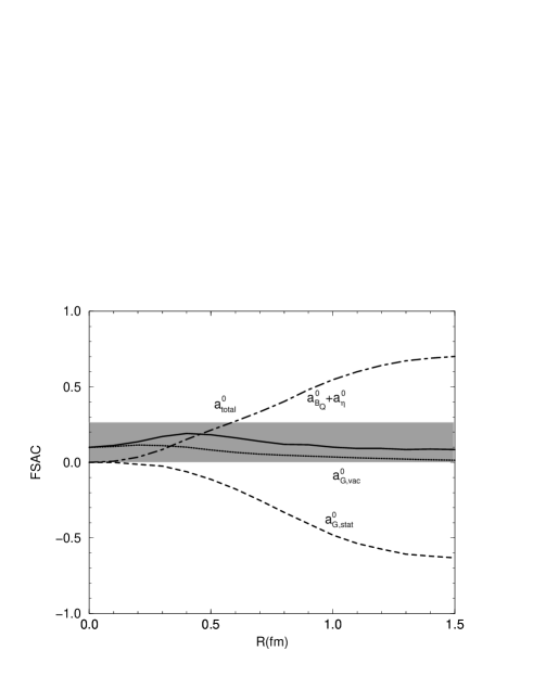
Figure 2: Various contributions to the flavor singlet axial current of the proton as a function of bag radius and comparison with the experiment: (a) quark plus $\eta$ (or “matter”) contribution ($a^{0}_{B_{Q}}+a^{0}_{\eta}$), (b) the contribution of the static gluons due to quark source ($a^{0}_{G,stat}$), (c) the gluon Casimir contribution ($a^{0}_{G,vac}$), and (d) their sum ($a^{0}_{total})$. The shaded area corresponds to the range admitted by experiments.

Let us turn to the gluon contribution. The gluon current is split into two pieces

$$A^{\mu}_{B_{G}}=A^{\mu}_{G,stat}+A^{\mu}_{G,vac}.$$ (I.130)

The first term arises from the quark and $\eta$ sources, while the latter is associated with the properties of the vacuum of the model. One might worry that this contribution could not be split into these two terms without double counting. However this worry is unfounded. Technically, it is easy to check it by noticing that the former acts on the quark Fock space and the latter on the gluon vacuum. Thus, one can interpret the former as a one gluon exchange correction to the quantity. One can also show this intuitively by making the analogy to the condensate expansion in QCD, where the perturbative terms and the vacuum condensates enter additively to the lowest order.

$\bullet$ The gluon static current $A^{\mu}_{G,stat}$

Let us first describe the static term.

We first ignore the $\eta$ coupling. Afterwards, the $\eta$ contribution can be added. The boundary conditions for the gluon field would correspond to the original MIT ones. The quark current is the source term that remains in the equations of motion after performing a perturbative expansion in the QCD coupling constant, i.e., the quark color current

$$g{\bar{\Psi}}_{0}\gamma_{\mu}\lambda^{a}\Psi_{0}$$ (I.131)

where the $\Psi_{0}$ fields represent the lowest cavity modes. In this lowest mode approximation, the color electric and magnetic fields are given by

$$\vec{E}^{a}=g_{s}\frac{\lambda^{a}}{4\pi}\frac{\hat{r}}{r^{2}}\rho(r)$$ (I.132)

$$\vec{B}^{a}=g_{s}\frac{\lambda^{a}}{4\pi}\left(\frac{\mu(r)}{r^{3}}(3\hat{r}\vec{\sigma}\cdot\hat{r}-\vec{\sigma})+(\frac{\mu(R)}{R^{3}}+2M(r))\vec{\sigma}\right)$$ (I.133)

where $\rho$ is related to the quark density $\rho^{\prime}$ as

$$\rho(r,\Gamma)=\int_{\Gamma}^{r}ds\rho^{\prime}(s)$$

and $\mu,M$ to the vector current density

$$\mu(r) = \int_{0}^{r}ds\mu^{\prime}(s),$$

$$M(r) = \int_{r}^{R}ds\frac{\mu^{\prime}(s)}{s^{3}}.$$

The lower limit $\Gamma$ is taken to be zero in the MIT bag model – in which case the boundary condition is satisfied only globally, that is, after averaging – and $\Gamma=R$ in the so called monopole solution – in which case, the boundary condition is satisfied locally. We take the latter since consistency with the CCP condition rules out the MIT condition.

We now proceed to introduce the $\eta$ field. We perform the same calculation with however the color boundary conditions Eqs.(I.96) and (I.97) taken into account. In the approximation of keeping the lowest non-trivial term, the boundary conditions become

$$\hat{r}\cdot\vec{E}_{stat}^{a}=\frac{N_{F}g^{2}}{8\pi^{2}f}\hat{r}\cdot\vec{B}^{a}_{g}\eta(R)$$ (I.134)

$$\hat{r}\times\vec{B}_{stat}^{a}=-\frac{N_{F}g^{2}}{8\pi^{2}f}\hat{r}\times\vec{E}^{a}_{g}\eta(R).$$ (I.135)

Here $\vec{E}^{a}_{g}$ and $\vec{B}^{a}_{g}$ are the lowest order fields given by (I.132) and (I.133) and $\eta(R)$ is the meson field at the boundary. The $\eta$ field is given by

$$\eta(\vec{r})=-\frac{g_{NN\eta}}{4\pi M}\vec{S}\cdot\hat{r}\frac{1+m_{\eta}r}{r^{2}}e^{-m_{\eta}r}$$ (I.136)

where the coupling constant is determined from the surface conditions.

Note that the magnetic field is not affected by the new boundary conditions, since $\vec{E}^{a}_{g}$ points into the radial direction. The effect on the electric field is just a change in the charge, i.e.,

$$\rho_{stat}(r)=\rho(r,\Gamma)+\rho_{\eta}(R)$$ (I.137)

where

$$\rho_{\eta}(R)=\frac{N_{F}g^{2}}{64\pi^{3}M}\frac{g_{NN\eta}}{f}(1+y_{\eta})e^{-y_{\eta}}.$$ (I.138)

The contribution to the FSAC arising from these fields is determined from the expectation value of the anomaly

$$a^{0}_{G,stat}=\langle p|-\frac{N_{F}\alpha_{s}}{\pi}\int_{B}d^{3}rx_{3}\vec{E}^{a}_{stat}\cdot\vec{B}^{a}_{stat}|p\rangle.$$ (I.139)

One finds that including the $\eta$ contribution in $\rho_{stat}(r)$ brings a non-negligible modification to the FSAC but does not modify the result qualitatively. The result as one can see in Fig. 2 shows that this contribution is zero at $R=0$ but increases as $R$ increases but with the sign opposite to that of the matter field, largely cancelling the $R$ dependence of the matter contribution. We should remark here that there is a drastic difference between the effect of the MIT-like electric field and that of the monopole-like electric field: The former is totally incompatible with the Cheshire Cat property whereas the latter remains consistent independently of whether or not the $\eta$ contribution is included in $\rho_{stat}$.

$\bullet$ The gluon Casimir current $A^{\mu}_{G,vac}$

Up to this point, the FSAC is zero for $R=0$ and non-zero for $R\neq 0$. This is in principle a violation of the CCP although the magnitude of the violation is small. We now show that it is the vacuum contribution through Casimir effects that the CCP is restored. The calculation is subtle involving renormalization of the Casimir effects, the details of which are to be found in [138]. Here we summarize the salient feature of the contribution.

The quantity to calculate is the gluon vacuum contribution to the flavor singlet axial current of the proton, which can be gotten by evaluating the expectation value

$$\langle 0_{B}|-\frac{N_{F}\alpha_{s}}{\pi}\int_{V}d^{3}rx_{3}(\vec{E}^{a}\cdot\vec{B}^{a})|0_{B}\rangle$$ (I.140)

where $|0_{B}\rangle$ denotes the vacuum in the bag. To calculate this, we invoke at this point the CCP which states that at low energy, hadronic phenomena do not discriminate between QCD degrees of freedom (quarks and gluons) on the one hand and meson degrees of freedom (pions, etas,…) on the other, provided that all necessary quantum effects (e.g., quantum anomalies) are properly taken into account. If we consider the limit where the $\eta$ excitation is a long wavelength oscillation of zero frequency, the CCP asserts that it does not matter whether we choose to describe the $\eta$, in the interior of the infinitesimal bag, in terms of quarks and gluons or in terms of mesonic degrees of freedom. This statement, together with the color boundary conditions, leads to an extremely simple and useful local formula [23, 135],

$$\vec{E}^{a}\cdot\vec{B}^{a}\approx-\frac{N_{F}g^{2}}{8\pi^{2}}\frac{\eta}{f}\frac{1}{2}G^{2},$$ (I.141)

where only the term up to the first order in $\eta$ is retained in the right-hand side. Here we adapt this formula to the CBM. This means that the couplings are to be understood as the average bag couplings and the gluon fields are to be expressed in the cavity vacuum through a mode expansion. That the surface boundary condition can be interpreted as a local operator is a rather strong CCP assumption which while justifiable for small bag radius, can only be validated a posteriori by the consistency of the result. This procedure is the substitute to the condensates in the conventional discussion.

Substituting Eq.(I.141) into Eq.(I.140) we obtain

$$\hskip-20.00003pt\langle 0_{B}|-\frac{N_{F}\alpha_{s}}{\pi}\int_{V}d^{3}rx_{3}(\vec{E}^{a}\cdot\vec{B}^{a})|0_{B}\rangle$$

$$\approx\left(-\frac{N_{F}\alpha_{s}}{\pi}\right)\left(-\frac{N_{F}g^{2}}{8\pi^{2}}\right)\frac{y(R)}{f_{0}}\langle p|S_{3}|p\rangle(N_{c}^{2}-1)$$

$$\hskip 30.00005pt\sum_{n}\int_{V}d^{3}r(\vec{B}_{n}^{*}\cdot\vec{B}_{n}-\vec{E}_{n}^{*}\cdot\vec{E}_{n})x_{3}\hat{x}_{3},$$ (I.142)

where we have used that $\eta$ has a structure of $(\vec{S}\cdot\hat{r})y(R)$. Since we are interested only in the first order perturbation, the field operator can be expanded by using MIT bag eigenmodes (the zeroth order solution). Thus, the summation runs over all the classical MIT bag eigenmodes. The factor $(N_{c}^{2}-1)$ comes from the sum over the abelianized gluons.

The next steps are the numerical calculations to evaluate the mode sum appearing in Eq.(I.142): (i) introduction of the heat kernel regularization factor to classify the divergences appearing in the sum and (ii) subtraction of the ultraviolet divergences. These procedures – which involve an intricate manipulation – are described in [138]. The result is shown in Fig. 2. Though the magnitude is small compared with the others, it is important at small $R$ to restore, within the CBM scheme, the CCP.

The lesson from this calculation is that neither the matter contribution nor the gluon contribution to $a^{0}$, both of which non-gauge-invariant and CCP-violating, is physical. Only the total which is gauge invariant is physical and CCP-preserving.

2 Induced (Berry) Gauge Fields in Hadrons

[Updating remark]

[In this section, the notion that “hidden gauge symmetries” may be induced as geometrical Berry phases was explored. Although the notion was attractive, no further developments were made in this direction. Let me just mention that the ultimate objective which was to obtain the observed vector degrees of freedom, namely, the vector mesons, as “emergent gauge degrees of freedom” is in line with the ambitious program of attempting to arrive at fundamental theories as “emergent” from collective phenomena as in condensed matter physics, see, e.g., [139, 140]. Perhaps related to this is the observation I will make later in connection with the notion that the low-energy light-quark vector mesons are equivalent to the gluons “dressed” with cloud of collective degrees of freedom, e.g., pions. This will be addressed in terms of color-flavor-locking in QCD.]

In this section, we introduce another aspect of the Cheshire Cat mechanism which generalizes the concept to excitations. So far our focus has been on the ground-state properties. That topological quantities satisfy the CCP exactly even in (3+1) dimensions (such as the baryon charge) is not surprising. This is a ground-state property associated with symmetry. It is a different matter when one wants to establish an approximate CCP for dynamical properties such as excitations, responses to external fields etc. To establish that certain response functions can be formulated in terms of effective variables, it proves to be highly fruitful to introduce and exploit the notion of induced gauge fields familiar in other areas of physics [29]. In this section, we discuss how a hierarchy of “vector-field” degrees of freedom can be induced and how they can lead to a natural setting for describing excited states and their dynamic properties[30]. Since the resulting structure is quite generic, we will spend some time discussing simpler quantum mechanical systems. When the dust settles, we will see that much of the arguments used for those systems can be applied with little modifications to hadronic systems.

2.1 “Magnetic Monopoles” in Flavor Space

A useful concept in understanding baryon excitations is the concept of induced magnetic monopoles and instantons, viz, topological objects, in order-parameter or in our case flavor space. First we consider a toy model, the quantum mechanical spin-solenoid system à la Stone [31] which succinctly illustrates the emergence of a Berry phase.

2.1.1 A Toy Model: (0+1) Dimensional Field Theory

Consider a system of a slowly rotating solenoid coupled to a fast spinning object (call it “electron”) described by the (Euclidean) action

$$S_{E}=\int dt\left(\frac{{\cal I}}{2}\dot{\vec{n}}^{2}+\psi^{\dagger}(\partial_{t}-\mu\hat{n}\cdot\vec{\sigma})\psi\right)$$ (I.143)

where $n^{a}(t)$, $a$=1,2,3, is the rotator with $\vec{n}^{2}=1$, ${\cal I}$ its moment of inertia, $\psi$ the spinning object (“electron”) and $\mu$ a constant. We will assume that $\mu$ is large so that we can make an adiabatic approximation in treating the slow-fast degrees of freedom. We wish to calculate the partition function

$$Z=\int[d\vec{n}][d\psi][d\psi^{\dagger}]\delta(\vec{n}^{2}-1)e^{-S_{E}}$$ (I.144)

by integrating out the fast degree of freedom $\psi$ and $\psi^{\dagger}$. Formally this yields the familiar fermion determinant, the evaluation of which is tantamount to doing the physics of the system. In adiabatic approximation, this can be carried out as follows which brings out the essence of the method useful for handling the complicated situations which will interest us later.

Imagine that $\vec{n}(t)$ rotates slowly. At each instant $t=\tau$, we have an instantaneous Hamiltonian $H(\tau)$ which in our case is just $-\mu\vec{\sigma}\cdot\hat{n}(\tau)$ and the “snap-shot” electron state $|\psi_{0}(\tau)\rangle$ satisfying

$$H(\tau)|\psi^{0}(\tau)\rangle=\epsilon(\tau)|\psi^{0}(\tau)\rangle.$$ (I.145)

In terms of these “snap-shot” wave functions, the solution of the time-dependent Schrödinger equation

$$i\partial_{t}|\psi(t)\rangle=H(t)|\psi(t)\rangle$$ (I.146)

is

$$|\psi(t)\rangle=e^{i\gamma(t)-i\int_{0}^{t}\epsilon(t^{\prime})dt^{\prime}}|\psi^{0}(t)\rangle.$$ (I.147)

Note that this has, in addition to the usual dynamical phase involving the energy $\epsilon(t)$, a nontrivial phase $\gamma(t)$ which substituted into (I.146) is seen to satisfy

$$i\frac{d\gamma}{dt}+\langle\psi^{0}|\frac{d}{dt}\psi^{0}\rangle=0.$$ (I.148)

This allows us to do the fermion path integrals to the leading order in adiabaticity and to obtain (dropping the trivial dynamical phase involving $\epsilon$)

$$Z=const\int[d\vec{n}]\delta(\vec{n}^{2}-1)e^{-S^{eff}},$$ (I.149)

$$S^{eff}(\vec{n})=\int{\cal L}^{eff}=\int[\frac{{\cal I}}{2}\dot{\vec{n}}^{2}-i\vec{{\cal A}}(\vec{n})\cdot\dot{\vec{n}}]dt$$

where

$$\vec{{\cal A}}(\vec{n})=\langle\psi^{0}(\vec{n})|i\frac{\partial}{\partial\vec{n}}\psi^{0}(\vec{n})\rangle$$ (I.150)

in terms of which $\gamma$ is

$$\gamma=\int\vec{{\cal A}}\cdot d\vec{n}.$$ (I.151)

${\cal A}$ so defined is known as Berry potential or connection and $\gamma$ is known as Berry phase [32]. That ${\cal A}$ is a gauge field with coordinates defined by $\vec{n}$ can be seen as follows. Under the transformation

$$\psi^{0} \rightarrow e^{i\alpha(\vec{n})}\psi^{0},$$ (I.152)

$\vec{{\cal A}}$ transforms as

$$\vec{{\cal A}} \rightarrow \vec{{\cal A}}-\frac{\partial}{\partial\vec{n}}\alpha(\vec{n})$$ (I.153)

which is just a gauge transformation. The theory is gauge-invariant in the sense that under the transformation (I.153), the theory (I.149) remains unchanged. (We are assuming that the surface term can be dropped.)

One should note that the gauge field we have here is first of all defined in “order parameter space”, not in real space like electroweak field or gluon field and secondly it is induced when fast degrees of freedom are integrated out. This is a highly generic feature we will encounter time and again. Later on we will see that the space on which the gauge structure emerges is usually the flavor space like isospin or hypercharge space in various dimensions.

We shall now calculate the explicit form of the potential ${\cal A}$. For this let us use the polar coordinate and parameterize the solenoid as

$$\vec{n}=(\sin\theta\cos\phi,\sin\theta\sin\phi,\cos\theta)$$ (I.154)

with the Euler angles $\theta(t)$ and $\phi(t)$ assumed to be slowly changing (slow compared with the scale defined by the fermion mass $\mu$) as a function of time. Then the relevant Hamiltonian can be written as

$$\delta H=-\mu\vec{\sigma}\cdot\hat{n}(t)=S(t)\delta H_{0}S^{-1}(t),$$ (I.155)

$$\delta H_{0}\equiv-\mu\sigma_{3}$$

with

$$S(\vec{n}(t))=\left(\matrix{\cos\frac{\theta}{2}&-\sin\frac{\theta}{2}e^{-i\phi}\cr\sin\frac{\theta}{2}e^{i\phi}&\cos\frac{\theta}{2}\cr}\right).$$ (I.156)

Since the eigenstates of $\delta H_{0}$ are $\left(\matrix{1\cr 0\cr}\right)$ with eigenvalue $-\mu$ and $\left(\matrix{0\cr 1\cr}\right)$ with eigenvalue $+\mu$, we can write the “snap-shot” eigenstate of $H(t)$ as

$$|\psi^{0}_{+\uparrow}\rangle=S\left(\matrix{1\cr 0\cr}\right)=\left(\matrix{\cos\frac{\theta}{2}\cr\sin\frac{\theta}{2}e^{i\phi}}\right)$$ (I.157)

where the arrow in the subscript denotes the “spin-up” eigenstate of $\delta H_{0}$ and $+$ denotes the upper hemisphere to be specified below. The eigenstate $|\psi^{0}_{+\downarrow}\rangle$ is similarly defined with the “down spin”. Now note that for $\theta=\pi$, (I.157) depends on $\phi$ which is undefined. This means that (I.157) is ill-defined in the lower hemisphere with a string singularity along $\theta=\pi$. On the other hand, (I.157) is well-defined for $\theta=0$ and hence in the upper hemisphere. The meaning of the $+$ in (I.157) is that it has meaning only in the upper hemisphere, thus the name “wave section” referring to it rather than wave function.

Given (I.157), we can use the definition (I.150) for the Berry potential to obtain

$$\vec{{\cal A}}_{+}(\vec{n})\cdot d\vec{n}=\langle\uparrow|S^{-1}dS|\uparrow\rangle=\frac{-1}{2}(1-\cos\theta)d\phi$$ (I.158)

written here in one-form. The explicit form of the potential is

$$\vec{{\cal A}}_{+}=-\frac{1/2}{(1+\cos\theta)}(-\sin\theta\sin\phi,\sin\theta\cos\phi,0)$$ (I.159)

which is singular at $\theta=\pi$ as mentioned above. This is the well-known Dirac string singularity. Since we have the gauge freedom, we are allowed to do a gauge transformation

$$\psi^{0}_{+}\rightarrow e^{-\phi}\psi^{0}_{+}\equiv\psi^{0}_{-}$$ (I.160)

which is equivalent to defining a gauge potential regular in the lower hemisphere (denoted with the subscript $-$)

$$\vec{{\cal A}}_{-}\cdot d\vec{n}=\vec{{\cal A}}_{+}\cdot d\vec{n}+d\phi$$ (I.161)

giving

$$\vec{{\cal A}}_{-}\cdot d\vec{n}=\frac{1}{2}(1+\cos\theta)d\phi.$$ (I.162)

This potential has a singularity at $\theta=0$. Thus we have gauge-transformed the Dirac string from the lower hemisphere to the upper hemisphere. This clearly shows that the string is an artifact and is unphysical. In other words, physics should not be dependent on the string. Indeed the field strength tensor, given in terms of the wedge symbol and forms,

$${\cal F}=d{\cal A}=\frac{1}{2}d\theta\wedge d\phi=\frac{1}{2}d(Area)$$ (I.163)

is perfectly well-defined in both hemispheres and unique. A remarkable fact here is that the gauge potential or more properly the field tensor is completely independent of the fermion “mass” $\mu$. This means that the potential does not depend upon how fast the fast object is once it is decoupled adiabatically. This indicates that the result may be valid even if the fast-slow distinction is not clear-cut. We will come back to this matter in connection with applications to the excitation spectra of the light-quark baryons.

We now explain the quantization rule. For this consider a cyclic path. We will imagine that the solenoid is rotated from $t=0$ to $t=T$ with large $T$ such that the parameter $\vec{n}$ satisfies $\vec{n}(0)=\vec{n}(T)$. We are thus dealing with an evolution, with the trajectory of $\vec{n}$ defining a circle $C$. The parameter space manifold is two-sphere $S^{2}$ since $\vec{n}^{2}=1$. Call the upper hemisphere $D$ and the lower hemisphere $\bar{D}$ whose boundary is the circle $C$, i.e, $\partial D=C$. Then using Stoke’s theorem, we have from (I.151) for a cyclic evolution $\Gamma$

$$\gamma(\Gamma)=\int_{C=\partial D}\vec{{\cal A}}\cdot d\vec{n}\equiv\int_{\partial D=C}{\cal A}=-\int_{D}d{\cal A}=-\int_{D}{\cal F}.$$ (I.164)

Since the gauge field in $\bar{D}$ is related to that in $D$ by a gauge transform, we could equally well write $\gamma$ in terms of the former. Thus we deduce that

$$e^{i\int_{C}{\cal A}}=e^{i\int_{D}{\cal F}}=e^{-i\int_{\bar{D}}{\cal F}}$$ (I.165)

which implies

$$e^{i\int_{D+\bar{D}=S^{2}}{\cal F}}=1.$$ (I.166)

Thus we get the quantization condition

$$\int_{S^{2}}{\cal F}=2\pi n$$ (I.167)

with $n$ an integer. This just means that the total “magnetic flux” going through the surface is quantized. Since in our case the field strength is given by (I.163), our system corresponds to $n=1$ corresponding to a “monopole charge” $g=1/2$ located at the center of the sphere. What we learn from the above exercise is that consistency with quantum mechanics demands that it be a multiple of 1/2. Otherwise, the theory makes no sense. It will turn out later that real systems in the strong interactions involve nonabelian gauge fields which do not require such “charge” quantization, making the consideration somewhat more delicate.

We should point out another way of looking at the action (I.143) which is useful for understanding the emergence of Berry potentials in more complex systems. Since

$$\hat{n}(t)\cdot\vec{\sigma}=S(t)\sigma_{3}S^{-1}(t)$$ (I.168)

we make the field redefinition

$$\psi\rightarrow\psi^{\prime}=S^{-1}(t)\psi.$$ (I.169)

Then (I.143) can be rewritten as

$$S_{E}=S_{E}^{0}+\int dt\psi^{\dagger}(S^{-1}\partial_{t}S)\psi.$$ (I.170)

Here the first term contains no coupling between the fast and slow degrees of freedom. The second term linear in time derivative generates the Berry structure analyzed above. We will encounter this structure in complex systems.

2.1.2 Connection to the WZW term

The key point which will be found useful later is this: when the fast degree of freedom (the “electron”) is integrated out, we wind up with a gauge field as a relic of the fast degree of freedom that is integrated out. The effective Lagrangian that results has the form (in Minkowski space)

$$L^{eff}=\frac{1}{2}{\cal I}\dot{\vec{n}}^{2}+{\vec{{\cal A}}}(\vec{n})\cdot\dot{\vec{n}}.$$ (I.171)

We now show that the Berry structure is closely related to what is called the Wess-Zumino-Witten term defined in two dimensions. For this, we recall that the gauge field in (I.171) is an induced one, coming out of the solenoid $\vec{n}$. Therefore one should be able to rewrite the second term of (I.171) in terms of $\vec{n}$ alone. However this cannot be done locally because of the Dirac singularity mentioned above but the corresponding action can be written locally in terms of $\vec{n}$ by extending (homotopically) to one dimension higher. This is the (one-dimensional) WZW term. When written in this way, the gauge structure will be “hidden” in some sense.

Let us look at the action

$$S_{WZ}\equiv\int\vec{{\cal A}}(\vec{n})\cdot\dot{\vec{n}}dt.$$ (I.172)

We have already shown how to express this in a local form. We repeat here to bring the point home. The general procedure goes as follows. First extend the space from the physical dimension $d$ which is 1 in our case to $d+1$ dimension. This extension is possible (“no obstruction”) if

$$\pi_{d}({\cal M})=0,\ \ \ \pi_{d+1}({\cal M})\neq 0$$ (I.173)

where $\pi$ is the homotopy group and ${\cal M}$ is the parameter space manifold. In our case

$$\pi_{1}(S^{2})=0,\ \ \ \pi_{2}(S^{2})=Z.$$ (I.174)

So it is fine. We therefore extend the space to $\tilde{n}(s)$, $0\leq s\leq 1$ such that

$$\tilde{n}(s=0)=1,\ \ \ \tilde{n}(s=1)=\vec{n}.$$ (I.175)

Now the next step is to construct a winding number density $\tilde{Q}$ for $\pi_{d+1}$ which is then to be integrated over a region of ${\cal M}$ ($\approx S^{2}$ here) bounded by d-dimensional fields $n^{i}$. The winding number density $\tilde{Q}(x)$ (say $x_{1}=t$ and $x_{2}=s$) is

$$\tilde{Q}=\frac{1}{8\pi}\epsilon^{ij}\epsilon^{abc}\tilde{n}^{a}\partial_{i}\tilde{n}^{b}\partial_{j}\tilde{n}^{c}$$ (I.176)

and the winding number $n$ (which is 1 for $\pi\leq\theta\leq 0$, $2\pi\leq\phi\leq 0$)

$$n=\int_{S^{2}}d^{2}x\tilde{Q}(x).$$ (I.177)

Comparing with (I.167), we deduce

$$S_{WZ}=4\pi g\int_{{{{\cal D}}}=t\times[0,1]}d^{2}x\tilde{Q}(x).$$ (I.178)

This is the familiar form of the WZW term defined in two dimensions. As we saw before this has a “monopole charge” $g=1/2$. Below we will carry $g$ as an integral multiple of 1/2. This way of understanding the WZW term complements the approach given in subsection 2.1.3 and brings out the universal characteristic of Berry phases.

2.1.3 Quantization

There are numerous ways of quantizing the effective action (hereon we will work in Minkowski space)

$$S^{eff}=S_{0}+S_{WZ}$$ (I.179)

where the Wess-Zumino action is given by (I.178) and

$$S_{0}=\oint dt\,\frac{{\cal I}}{2}\,\dot{\vec{n}}^{2}.$$ (I.180)

We will consider the time compactified as defined above, so the time integral is written as a loop integral. We will choose one way [33] which illustrates other interesting properties.

The manifold has $SO(3)$ invariance corresponding to $\sum_{i=1}^{3}n_{i}^{2}=1$. Consider now the complex doublet $z\in SU(2)$

$$z(t)=\left(\matrix{z_{1}\cr z_{2}\cr}\right),$$ (I.181)

$$z^{\dagger}z=|z_{1}|^{2}+|z_{2}|^{2}=1.$$ (I.182)

Then we can write

$$n_{i}=z^{\dagger}\sigma_{i}z$$ (I.183)

with $\sigma_{i}$ the Pauli matrices. There is a redundant (gauge) degree of freedom since under the $U(1)$ transformation $z\rightarrow e^{i\alpha}z$, $n_{i}$ remains invariant. This is as it should be since the manifold is topologically $S^{2}$ and hence corresponds to the coset $SU(2)/U(1)$. We are going to exploit this $U(1)$ gauge symmetry to quantize our effective theory.

Define a 2-by-2 matrix $h$

$$h=\left(\matrix{z_{1}&-z_{2}^{\star}\cr z_{2}&z_{1}^{\star}}\right)$$ (I.184)

and

$$a(t)=\sum_{k=1}^{2}\frac{i}{2}(z_{k}^{\star}\stackrel{{\scriptstyle\leftrightarrow}}{{\partial}}_{k}z_{k}).$$ (I.185)

Then it is easy to obtain (setting ${\cal I}=1$) that

$$S_{0}=\frac{1}{2}\oint\!dt{\rm Tr}\left[\stackrel{{\scriptstyle\rightarrow}}{{D}}_{t}^{\dagger}h^{\dagger}h\stackrel{{\scriptstyle\leftarrow}}{{D}}_{t}\right]$$ (I.186)

where

$$\stackrel{{\scriptstyle\rightarrow}}{{D}}_{t}=\stackrel{{\scriptstyle\rightarrow}}{{\partial}}_{t}-ia\sigma_{3}.$$ (I.187)

Let

$$\tilde{a}_{\mu}=\frac{i}{2}(\tilde{z}_{k}^{\star}\stackrel{{\scriptstyle\leftrightarrow}}{{\partial}}_{\mu}\tilde{z}_{k})$$ (I.188)

where the index $\mu$ runs over the extended coordinate $(s,t)$. As noted before, there is no topological obstruction to this extension. This is defined in such a way that $\tilde{z}(s=0)=1$ and $\tilde{z}(s=1)=z$. Then the Wess-Zumino action can be written in a Chern-Simons form

$$S_{WZ}=2g\int_{{{\cal D}}}d^{2}x\epsilon^{\mu\nu}\partial_{\mu}\tilde{a}_{\nu}=2g\oint\!dta(t).$$ (I.189)

Introducing an auxiliary function $A$, we can write the partition function

$$Z=\int[dz][dz^{\dagger}][dA]exp\ i\oint dt\left(\frac{1}{2}{\mbox{Tr}}(\stackrel{{\scriptstyle\rightarrow}}{{\partial}}_{t}+iA\sigma_{3})h^{\dagger}h(\stackrel{{\scriptstyle\leftarrow}}{{\partial}}_{t}-iA\sigma_{3})+2gA+\frac{1}{4}(2g)^{2}\right).$$ (I.190)

The $U(1)$ gauge invariance is manifest in this action. Indeed if we make the (local) transformation $h\rightarrow e^{i\alpha(t)\frac{\sigma_{3}}{2}h}$ and $A\rightarrow A-\frac{1}{2}\partial_{t}\alpha(t)$ with the boundary condition $\alpha(T)-\alpha(0)=4\pi N$ where $N$ is an integer, then the action remains invariant. This means that we have to gauge-fix the “gauge field” $A$ in the path integral. The natural gauge choice is the “temporal gauge” $A=0$. The resulting gauge-fixed action is $\oint{\cal L}_{gf}$ with

$${\cal L}_{gf}={\mbox{Tr}}(\partial_{t}h^{\dagger}\partial_{t}h)+g^{2}.$$ (I.191)

Since there is no time derivative of $A$ in (I.190), there is a Gauss’ law constraint which is obtained by taking $\frac{\delta S}{\delta A}|_{A=0}$ from the action (I.190) before gauge fixing:

$$\frac{i}{2}{\mbox{Tr}}\left(\sigma_{3}h^{\dagger}\partial_{t}h-\partial_{t}h^{\dagger}h\sigma_{3}\right)+2g=0$$

which is

$$i{\mbox{Tr}}\left(\partial_{t}h^{\dagger}h\frac{\sigma_{3}}{2}\right)=g.$$ (I.192)

The left-hand side is identified as the right rotation around third axis $J_{3}^{R}$, so the constraint is that

$$J_{3}^{R}=g.$$ (I.193)

Since (I.191) is invariant under $SU(2)_{L,R}$ multiplication, we have that

$$\vec{J}^{2}=\vec{J}_{L}^{2}=\vec{J}_{R}^{2}.$$ (I.194)

The Hamiltonian is (restoring the moment of inertia ${\cal I}$)

$$H=\frac{1}{2{\cal I}}\left(\vec{J}^{2}-g^{2}\right)$$ (I.195)

which has the spectrum of a tilted symmetric top. Now adding the energy of the “electron”, the total energy is

$$E=\epsilon+\frac{1}{2{\cal I}}\left(J(J+1)-g^{2}\right)$$ (I.196)

with the allowed values for $J$

$$J=|g|,|g|+1,\cdots.$$ (I.197)

The rotational spectrum is the well-known Dirac monopole spectrum. Later we will derive an analogous formula for real systems in four dimensions. The corresponding wavefunction is given by monopole harmonics.

Summary

When a fast spinning object coupled to slowly rotating object is integrated out, a Berry potential arises gauge-coupled to the rotor. The effect of this gauge coupling is to “tilt” the angular momentum of the rotor in the spectrum of a symmetric top. It supplies an extra component to the angular momentum, along the third direction. The gauge field is abelian and has an abelian (Dirac) monopole structure. The abelian nature is inherited from one nondegenerate level crossing another nondegenerate level. When degenerate levels cross, the gauge field can be nonabelian and this is the generic feature we will encounter in strong interaction physics.

2.2 Induced Nonabelian Gauge Field

2.2.1 Diatomic Molecules in Born-Oppenheimer approximation

In hadronic systems we will study below, we typically encounter nonabelian induced gauge potentials. This is because degeneracy is present. In order to understand this situation, we first discuss here a case in which a nonabelian gauge structure arises in a relatively simple quantum mechanical system. To do so, we will study a simple toy-model example of the induced nonabelian gauge fields and Berry phases in the Born-Oppenheimer approximation[34]. When suitably implemented, the treatment can be applied to a realistic description of the spectrum of a diatomic molecule, wherein this approximation is usually described as a separation of slow (nuclear) and fast (electronic) degrees of freedom. This separation is motivated by the fact that the rotation of the nuclei does not cause the transitions between the electron levels. In other words, the splittings between the fast variables are much larger than the splittings between the slow ones. We will demonstrate how the integrating-out of the fast degrees of freedom generates in the slow-variable space an induced vector potential of the Dirac monopole type in certain special situations.

Before we develop the main argument, we should mention one point which may not be clear at each stage of the development but should be kept in mind. In the strong interactions at low energy, it is not always easy to delineate the “fast” and “slow” degrees of freedom. In particular in the chiral (light-quark) systems that we shall consider later, it is not even clear whether it makes sense to make the distinction. Nonetheless we will see that once the delineation is made, whether it is sharp or not, the result does not depend on how good the distinction is. This was already clear from the quantum mechanics of the solenoid-spin system we discussed above where the final result had no memory of how strong the coupling of the spin to the solenoid – namely, the coefficient $\mu$ – was. In a later section where we deal with heavy-quark systems, we will see that there the concept developed here applies much better than in light-quark systems.

Let us define a generic Hamiltonian describing a system consisting of the slow (“nuclear”) variables $\vec{R}(t)$ (with $\vec{P}$ as conjugate momenta) and the fast (“electronic”) variables $\vec{r}$ (with $\vec{p}$ as conjugate momenta) coupled through a potential $V(\vec{R},\vec{r})$

$$H=\frac{\vec{P}^{2}}{2M}+\frac{\vec{p}^{2}}{2m}+V(\vec{R},\vec{r})$$ (I.198)

where we have reserved the capitals for the slow variables and lower-case letters for the fast variables. We expect the electronic levels to be stationary under the adiabatic (slow) rotation of the nuclei. We split therefore the Hamiltonian into the slow and fast parts,

$$H = \frac{\vec{P}^{2}}{2M}+h$$

$$h(\vec{R}) = \frac{\vec{p}^{2}}{2m}+V(\vec{r},\vec{R})$$ (I.199)

where the fast Hamiltonian $h$ depends parameterically on the slow variable $\vec{R}$. The snapshot Hamiltonian (for fixed $\vec{R}$) leads to the Schrödinger equation:

$$h\phi_{n}(\vec{r},\vec{R})=\epsilon_{n}(\vec{R})\phi_{n}(\vec{r},\vec{R})$$ (I.200)

with electronic states labelled by the set of quantum numbers $n$. The wave function for the whole system is

$$\Psi(\vec{r},\vec{R})=\sum_{n}\Phi_{n}(\vec{R})\phi_{n}(\vec{r},\vec{R}).$$ (I.201)

Substituting the wave function into the full Hamiltonian and using the equation for the fast variables we get

$$\sum_{n}\left[\frac{\vec{P}^{2}}{2M}+\epsilon_{n}(\vec{R})\right]\Phi_{n}(\vec{R})\phi_{n}(\vec{r},\vec{R})=E\sum_{n}\Phi_{n}(\vec{R})\phi_{n}(\vec{r},\vec{R})$$ (I.202)

where $E$ is the energy of the whole system. Note that the operator of the kinetic energy of the slow variables acts on both slow and fast parts of the wavefunction. We can now “integrate out” the fast degrees of freedom. A bit of algebra leads to the following effective Schrödinger equation

$$\sum_{m}H_{nm}^{eff}\Phi_{m}=E\Phi_{n}$$ (I.203)

where the explicit form of the matrix-valued Hamiltonian (with respect to the fast eigenvectors) is

$$H_{mn}^{eff}=\frac{1}{2M}\sum_{k}\vec{\Pi}_{nk}\vec{\Pi}_{km}+\epsilon_{n}\delta_{nm}$$ (I.204)

where

$$\vec{\Pi}_{nm}=\delta_{nm}\vec{P}-i<\phi_{n}(\vec{r},\vec{R})|\vec{\nabla}_{R}|\phi_{m}(\vec{r},\vec{R})>\equiv\delta_{mn}\vec{P}-\vec{A}_{nm}.$$ (I.205)

The above equation is exact. We see that the effect of the fast variables is summarized by an effective gauge field $\vec{A}$. The vector part couples minimally to the momenta with the fast eigenvalue acting like a scalar potential. The vector field is in general nonabelian and corresponds to a nonabelian Berry potential first discussed by Wilczek and Zee [35].

In case one can neglect the off-diagonal transition terms in the induced gauge potentials (i.e, if the adiabatic approximation is valid), then the Hamiltonian simplifies to

$$H_{n}^{eff}=\frac{1}{2M}(\vec{P}-\vec{A}_{n})^{2}+\epsilon_{n}$$ (I.206)

where the diagonal component of the Berry phase $A_{nn}$ is denoted by $A_{n}$. Suppose that the electronic eigenvalues are degenerate so that there are $G_{n}$ eigenvectors with a degenerate eigenvalue $\epsilon_{n}$. Then instead of a single Berry phase, we have a whole set of the $G_{n}\times G_{n}$ Berry phases, forming the matrix

$$A_{n}^{k,k^{{}^{\prime}}}=i<n,k|\nabla|n,k^{{}^{\prime}}>\,\,\,\,\,\,\,\,k,k^{{}^{\prime}}=1,2,...G_{n}.$$ (I.207)

The gauge field generated in such a case is nonabelian valued in the gauge group $U(G_{n})$. In practical calculations, one truncates the infinite sum in (I.201) to a few finite terms. Usually the sum is taken over the degenerate subspace corresponding to the particular eigenvalue $\epsilon_{n}$. This is so-called Born-Huang approximation, which we will use in what follows. (A Berry potential built of the whole space would be a pure gauge type and would have a vanishing stress tensor, so it would be trivial.)

As stated, the fast variable will be taken to be the motion of the electron around the internuclear axis. The slow variables are the vibrations and rotations of the internuclear axis. This case corresponds to the situation where the energy of the spin-axis interaction is large compared with the energy splittings between the rotational levels, so that the adiabaticity condition holds. This is called “Hund case a”. We follow the standard notation [36]: Introducing the unit vector $\vec{N}$ along the internuclear axis, we define then the following quantum numbers

$$\Lambda = \,\,{\rm eigenvalue\,\,\,of\,\,}\vec{N}\cdot\vec{L}$$

$$\Sigma = \,\,{\rm eigenvalue\,\,\,of\,\,}\vec{N}\cdot\vec{S}$$

$$\Omega = \,\,{\rm eigenvalue\,\,\,of\,\,}\vec{N}\cdot\vec{J}=|\Lambda+\Sigma|,$$ (I.208)

so $\Lambda,\Sigma,\Omega$ are the projections of the orbital momentum, spin and total angular momentum of the electron on the molecular axis, respectively. For simplicity we focus on the simple case of $\Sigma=0$, $\Lambda=0,\pm 1$. The $\Lambda=0$ state is referred to as $\Sigma$ state and the $\Lambda=\pm 1$ states are called $\pi$, a degenerate doublet. We are interested in the property of these triplet states, in particular in the symmetry associated with their energy splittings.

To analyze the model, let us write the Lagrangian corresponding to the Hamiltonian (I.206)

$$L_{nm}^{eff}=\frac{1}{2}M\dot{\vec{R}}(t)^{2}\delta_{mn}+\vec{A}_{mn}[\vec{R}(t)]\cdot\dot{\vec{R}}(t)-\epsilon_{m}\delta_{mn}.$$ (I.209)

This can be rewritten in non-matrix form (dropping the trivial electronic energy $\epsilon$)

$${\cal L}=\frac{1}{2}M\dot{\vec{R}}^{2}+i\theta^{\dagger}_{a}(\frac{\partial}{\partial t}-i\vec{A}^{\alpha}T^{\alpha}_{ab}\cdot\dot{\vec{R}})\theta_{b}$$ (I.210)

where we have introduced a Grassmannian variable $\theta_{a}$ as a trick to avoid using the matrix form of (I.209) [37] and ${\bf T}^{\alpha}$ is a matrix representation in the vector space in which the Berry potential lives satisfying the commutation rule

$$[{\bf T}^{\alpha},{\bf T}^{\beta}]=if^{\alpha\beta\gamma}{\bf T}^{\gamma}.$$ (I.211)

To get to (I.206) from this form of Lagrangian, we use the standard quantization procedure to obtain the following commutation relations,

$$[R_{i},p_{j}]=i\delta_{ij},\ \ \ \ \ \{\theta_{a},\theta_{b}^{\dagger}\}=i\delta_{ab}.$$ (I.212)

The Hamiltonian

$$H=\frac{1}{2M}(\vec{P}-\vec{{\bf A}})^{2}$$ (I.213)

follows with

$$\vec{{\bf A}} = \vec{A}^{\alpha}I^{\alpha},$$

$$I^{\alpha} = \theta^{\dagger}_{a}T^{\alpha}_{ab}\theta_{b}.$$ (I.214)

Using the commutation relations, it can be verified that

$$[I^{\alpha},I^{\beta}]=if^{\alpha\beta\gamma}I^{\gamma}.$$ (I.215)

The Lagrangian, Eq.(I.210), is invariant under the gauge transformation

$$\vec{A}^{\alpha} \rightarrow \vec{A}^{\alpha}+f^{\alpha\beta\gamma}\Lambda^{\beta}\vec{A}^{\gamma}-\vec{\nabla}\Lambda^{\alpha},$$ (I.216)

$$\theta_{a} \rightarrow \theta_{a}-i\Lambda^{\alpha}T^{\alpha}_{ab}\theta_{b}.$$ (I.217)

It should be noted that Eq.(I.217) corresponds to the gauge transformation on $|a\rangle$.

2.2.2 Conserved angular momentum of the nonabelian monopole

Before discussing structure of the diatomic molecular system, we digress here and review the known case of a particle coupled to an external gauge field of ’t Hooft-Polyakov monopole [38] with a coupling constant $g$ to which our nonabelian gauge field will correspond. Asymptotically the magnetic field involved is of the form

$$\vec{\bf B}=-\frac{\hat{r}(\hat{r}\cdot{\bf T})}{gr^{2}}$$ (I.218)

which is obtained from the asymptotic form of the gauge field $\vec{{\bf A}}$

$$A^{\alpha}_{i} = \epsilon_{\alpha ij}\frac{r_{j}}{gr^{2}},$$ (I.219)

$$\vec{{\bf B}} = \vec{\nabla}\times\vec{{\bf A}}-ig[\vec{{\bf A}},\vec{{\bf A}}].$$ (I.220)

The Hamiltonian of a particle coupled to a ’t Hooft-Polyakov monopole can therefore be written as

$$H = \frac{1}{2M}(\vec{p}-\vec{\bf A})^{2}$$ (I.221)

$$= \frac{1}{2M}\vec{{\bf D}}\cdot\vec{{\bf D}}$$

where $\vec{{\bf D}}=\vec{p}-\vec{\bf A}$.

It is obvious that the mechanical angular momentum $\vec{L}_{m}$ of a particle

$$\vec{L}_{m}=M\vec{r}\times\dot{\vec{r}}=\vec{r}\times\vec{{\bf D}}$$ (I.222)

does not satisfy the $SU(2)$ algebra after canonical quantization as in Eq.(I.212) and moreover it cannot be a symmetric operator that commutes with the Hamiltonian. The conventional angular momentum, $\vec{L}_{o}=\vec{r}\times\vec{p}$, satisfies the usual angular momentum commutation rule. However it does not commute with the Hamiltonian and hence cannot be a conserved angular momentum of the system. This observation shows us that the construction of a conserved angular momentum of a system coupled to a topologically nontrivial gauge field is not a trivial matter.

The conserved angular momentum can be constructed by modifying $\vec{L}_{m}$ to

$$\vec{L}=\vec{L}_{m}+\vec{{\bf Q}},$$ (I.223)

where $\vec{{\bf Q}}=\vec{Q}^{\alpha}I^{\alpha}$ is to be obtained as follows. The methods to determine $\vec{{\bf Q}}$ are standard [39]. The first condition required for $\vec{{\bf Q}}$ is the consistency condition that $\vec{L}$ satisfy the $SU(2)$ algebra

$$[L_{i},L_{j}]=i\epsilon_{ijk}L_{k}.$$ (I.224)

This leads to an equation for $\vec{{\bf Q}}$,

$$\vec{r}(\vec{r}\cdot\vec{{\bf B}})+\vec{r}\vec{{\cal D}}\cdot\vec{{\bf Q}}-\vec{{\cal D}}(\vec{r}\cdot\vec{{\bf Q}})=0.$$ (I.225)

where

$$\vec{{\cal D}}=\vec{\nabla}-i[\vec{{\bf A}},\ \ \ ].$$ (I.226)

The second equation is obtained by requiring that $\vec{L}$ commute with H,

$$[\vec{L},H]=0.$$ (I.227)

Eq.(I.227) can be replaced by a stronger condition

$$[L_{i},{\bf D}_{j}]=i\epsilon_{ijk}{\bf D}_{k},$$ (I.228)

which leads to

$${\cal D}_{i}{\bf Q}_{j}+\delta_{ij}\vec{r}\cdot\vec{{\bf B}}-r_{i}{\bf B}_{j}=0.$$ (I.229)

It is obvious that $\vec{L}$ satisfying Eq.(I.228) or (I.229) commutes with the Hamiltonian Eq.(I.221).

In the case of the ’t Hooft-Polyakov monopole, eqs.(I.218) and (I.219), it can be shown that

$$\vec{{\bf Q}}=\hat{r}(\hat{r}\cdot{\bf I})$$ (I.230)

satisfies eqs. (I.225) and (I.229). After inserting Eq.(I.230) into Eq.(I.223), we get

$$\vec{L} = \vec{L}_{m}+\hat{r}(\hat{r}\cdot{\bf I})$$ (I.231)

$$= \vec{r}\times\vec{p}+\vec{I},$$ (I.232)

where

$$I_{i}=\delta_{i\alpha}I^{\alpha}.$$ (I.233)

Equations (I.232, I.233) show clearly how the isospin-spin transmutation occurs in a system where a particle is coupled to a nonabelian monopole [40].

This analysis can be applied to the abelian $U(1)$ monopole just by replacing $\hat{r}\cdot\vec{I}$ by -1 in Eqs.(I.230) and (I.231). Then

$$\vec{Q} = \hat{r},$$ (I.234)

$$\vec{L} = m\vec{r}\times\dot{\vec{r}}-\hat{r}.$$ (I.235)

This can be rewritten as

$$\vec{L}=\vec{r}\times\vec{p}-\vec{\Sigma},$$ (I.236)

where

$$\vec{\Sigma}=\left(\frac{(1-\cos\theta)}{\sin\theta}\cos\phi,\,\frac{(1-\cos\theta)}{\sin\theta}\sin\phi,\,1\right)$$ (I.237)

which is the form frequently seen in the literature.

2.2.3 Symmetry and spectrum of the diatomic molecule

We now turn to the problem of constructing conserved angular momentum in a diatomic molecule in which a Berry potential couples to the dynamics of slow degrees of freedom, corresponding to the nuclear coordinate $\vec{R}$, a system that has been studied extensively [34]. The procedure is in complete parallel to that reviewed above.

As mentioned before, the Berry potential is defined on the space spanned by the electronic states $\pi(|\Lambda|=1)$ and $\Sigma(\Lambda=0)$, where $\Lambda$’s are eigenvalues of the third component of the orbital angular momentum of the electronic states. The electronic states responding to slow rotation of $\vec{R}$ described by $U(\vec{R})$,

$$U(\vec{R})={\rm exp}(-i\phi L_{z}){\rm exp}(i\theta L_{y}){\rm exp}(i\phi L_{z}),$$ (I.238)

induce a Berry potential of the form

$$\vec{{\bf A}} = i\langle\Lambda_{a}|U(\vec{R})\vec{\nabla}U(\vec{R})^{\dagger}|\Lambda_{b}\rangle$$ (I.239)

$$= \frac{{\bf A}_{\theta}}{R}\hat{{\bf\theta}}+\frac{{\bf A}_{\phi}}{R\sin\theta}\hat{{\bf\phi}},$$ (I.240)

where

$${\bf A}_{\theta} = \kappa(R)({\bf T}_{y}\cos\phi-{\bf T}_{x}\sin\phi),$$

$${\bf A}_{\phi} = {\bf T}_{z}(\cos\theta-1)-\kappa(R)\sin\theta({\bf T}_{x}\cos\phi+{\bf T}_{y}\sin\phi).$$ (I.241)

$\vec{{\bf T}}^{\prime}$s are spin-1 representations of the orbital angular momentum $\vec{L}$ and $\kappa$ measures the transition amplitude between the $\Sigma$ and $\pi$ states

$$\kappa(R)=\frac{1}{\sqrt{2}}|\langle\Sigma|L_{x}-iL_{y}|\pi\rangle|.$$ (I.242)

The nonvanishing field strength tensor is given by

$$\vec{{\bf B}}=\frac{F_{\theta\phi}}{R^{2}\sin\theta}=-\frac{(1-\kappa^{2})}{R^{2}}T_{z}\hat{R}.$$ (I.243)

Following the procedure described above, introducing a Grassmannian variable for each electronic state and replacing ${\bf T}$ by I defined in Eq.(I.214) and quantizing the corresponding Lagrangian, we obtain the Hamiltonian

$$H=\frac{1}{2M}(\vec{P}-\vec{{\bf A}})^{2},$$ (I.244)

where $\vec{{\bf A}}=\vec{A}^{\alpha}I^{\alpha}$. It should be noted that the presence of the constant $\kappa$ which is not quantized that appears in the Berry potential is a generic feature of nontrivial nonabelian Berry potentials as can be seen in many examples [29].

To find a solution of Eq.(I.225) and Eq.(I.229), we can exploit the gauge freedom and rewrite the Hamiltonian in the most symmetric form. This can be done by a gauge transform of the form

$$\vec{{\bf A}}^{\prime} = V^{\dagger}\vec{{\bf A}}V+iV^{\dagger}\vec{\nabla}V$$ (I.245)

$${\bf F}^{\prime} = V^{\dagger}{\bf F}V$$ (I.246)

where $V$ is an inverse operation of $U$ in Eq.(I.238), i.e., $V=U^{\dagger}$. Then

$${\bf A}_{\theta}^{\prime} = (1-\kappa)(I_{x}\sin\phi-I_{y}\cos\phi),$$

$${\bf A}_{\phi}^{\prime} = (1-\kappa)\{-I_{z}\sin^{2}\theta+\cos\theta\sin\theta(I_{x}\cos\phi+I_{y}\sin\phi)\},$$ (I.247)

or more compactly

$$\vec{{\bf A}}^{\prime}=(1-\kappa)\frac{\hat{R}\times\vec{I}}{R},$$

and

$$\vec{{\bf B}}^{\prime}=-(1-\kappa^{2})\frac{\hat{R}(\hat{R}\cdot{\bf I})}{R^{2}}.$$ (I.248)

It is remarkable that the above Berry potential has the same structure as the ’t Hooft-Polyakov monopole, Eq.(I.218) and Eq.(I.219), except for the different constant factors $(1-\kappa)$ for vector potential and $(1-\kappa^{2})$ for magnetic field. Because of these two different factors, however, one cannot simply take Eq.(I.230) as a solution of (I.229) for the case of nonabelian Berry potentials. Using the following identities derived from Eq. (I.247),

$$\vec{R}\cdot\vec{{\bf A}}^{\prime} = 0,$$ (I.249)

$$\vec{R}\times\vec{{\bf A}}^{\prime} = -(1-\kappa)\{\vec{I}-(\vec{I}\cdot\hat{R})\hat{R}\},$$ (I.250)

the Hamiltonian, Eq.(I.244), can be written as

$$H=-\frac{1}{2MR^{2}}\frac{\partial}{\partial R}R^{2}\frac{\partial}{\partial R}+\frac{1}{2MR^{2}}(\vec{L}_{o}+(1-\kappa)\vec{I})^{2}-\frac{1}{2MR^{2}}(1-\kappa)^{2}(\vec{I}\cdot\hat{R})^{2}.$$ (I.251)

Now one can show that the conserved angular momentum $\vec{L}$ is

$$\vec{L} = \vec{L}_{o}+\vec{I},$$ (I.252)

$$= M\vec{R}\times\dot{\vec{R}}+\vec{{\bf Q}},$$ (I.253)

with

$$\vec{{\bf Q}}=\kappa\vec{I}+(1-\kappa)\hat{R}(\hat{R}\cdot\vec{I}).$$ (I.254)

Hence, in terms of the conserved angular momentum $\vec{L}$, the Hamiltonian becomes

$$H=-\frac{1}{2MR^{2}}\frac{\partial}{\partial R}R^{2}\frac{\partial}{\partial R}+\frac{1}{2MR^{2}}(\vec{L}-\kappa\vec{I})^{2}-\frac{1}{2MR^{2}}(1-\kappa)^{2}$$ (I.255)

where $(\vec{I}\cdot\hat{R})^{2}=1$ has been used.

It is interesting to see what happens in the two extreme cases of $\kappa=0$ and $1$. For $\kappa=1$, the degenerate $\Sigma$ and $\pi$ states form a representation of the rotation group and hence the Berry potential (and its field tensor) vanishes or becomes a pure gauge. Then $\vec{{\bf Q}}=\vec{I}$ and $\vec{L}=M\vec{R}\times\dot{\vec{R}}+\vec{I}$. Now $\vec{I}$ can be understood as the angular momentum of the electronic system which is decoupled from the spectrum. One can also understand what happens here as the restoration of rotational symmetry in the electronic system. Physically $\kappa\rightarrow 1$ as $R\rightarrow\infty$.

For $\kappa=0$, the $\Sigma$ and $\pi$ states are completely decoupled and only the $U(1)$ monopole field can be developed on the $\pi$ states [41]. Equation (I.254) becomes identical to Eq.(I.234) as $\kappa$ goes to zero and the Hamiltonian can be written as

$$H=-\frac{1}{2MR^{2}}\frac{\partial}{\partial R}R^{2}\frac{\partial}{\partial R}+\frac{1}{2MR^{2}}(\vec{L}\cdot\vec{L}-1)$$ (I.256)

which is a generic form for a system coupled to an $U(1)$ monopole field. Physically this corresponds to small internuclear distance at which the $\Sigma$ and $\pi$ states decouple. Therefore, a truly nonabelian Berry potential can be obtained only for a $\kappa$ which is not equal to zero or one. We will encounter later an analogous situation in heavy-quark baryons.

2.3 Berry Phases in the Chiral Bag Model

2.3.1 Induced gauge fields

We now turn to hadronic systems in (3+1) dimensions and use the intuition we gained in the quantum mechanical cases, exploiting largely the generic structure of the resulting expressions. Consider the generating functional for the chiral bag in $SU(2)$ flavor space

$$Z=\int d[{\bf\pi}]\,d[\psi][\bar{\psi}]e^{iS}$$ (I.257)

with the (Minkowski) action S for the chiral bag given by

$$S=\int_{V}\,\overline{\psi}i\gamma^{\mu}\partial_{\mu}\psi-\frac{1}{2}\int\Delta_{s}\,\,\overline{\psi}\,S\,e^{i\gamma_{5}\vec{\tau}\cdot\hat{r}F(r)}\,S^{{\dagger}}\,\psi+S_{M}(SU_{0}S^{{\dagger}})$$ (I.258)

where $F$ is the chiral angle appearing in the “hedgehog” configuration $U_{0}=e^{i\vec{\tau}\cdot\hat{r}F(r)}$, $\Delta_{s}$ is a surface delta function and the space rotation has been traded in for an isospin rotation ($S(t)$) due to the hedgehog symmetry considered here. The quarks are assumed to be confined in the spatial volume $V$ and the purely mesonic terms outside the bag are described by $S_{M}$.

Suppose that we adiabatically rotate the bag in space. As we will see later, the “rotation” is required to quantize the zero modes to obtain the quantum states of the physical baryons. In this model, the rotation implies transforming the hedgehog configuration living outside the bag as

$$U_{0}\rightarrow S(t)U_{0}S^{\dagger}(t)$$ (I.259)

to which the quarks in the bag respond in a self-consistent way. This leads to computing the path integral in (I.257) with (I.258). Because of the degeneracy of the Dirac spectrum, mixing between quark levels is expected no matter how small the rotation is. This mixing takes place in each quark “grand spin” $K$-band (where $K$ is the vector sum of spin and isospin that labels hedgehog quark states) and leads to a nonabelian Berry or gauge field. Instead of the boundary term rotating as a function of time, it is more convenient to work with a static boundary condition by “unwinding” the boundary with the redefinition $\psi\rightarrow S\psi$, leading to

$$S=S_{S={\bf 1}}+\int\,{\psi}^{{\dagger}}\,{S}^{{\dagger}}i\partial_{t}S\,\psi\,.$$ (I.260)

The effect of the rotation on the fermions inside the bag is the same as a time dependent gauge potential. This is the origin of the induced Berry potential analogous to the solenoid-electron system described above. Now as the meson field outside rotates, the quarks inside the bag could either remain in their ground state which is in the lowest-energy $K=0^{+}$ orbit or excited to higher orbits. In the former case, we have a ground-state baryon and no Berry phases remain active: There is no Wess-Zumino term in the SU(2) case. In the latter case, as sketched in Fig. (3), there are, broadly, two classes of quark excitations that can be distinguished.

• Class A: One or more quarks get excited to $K\neq 0^{+}$ levels, changing no flavors;

• Class B: One or more quarks get excited to flavor Q levels through a flavor change where Q could be strange, charm or bottom quark.

In what follows, we will address the problem using Class A but the discussion applies equally well to Class B as we will detail later.

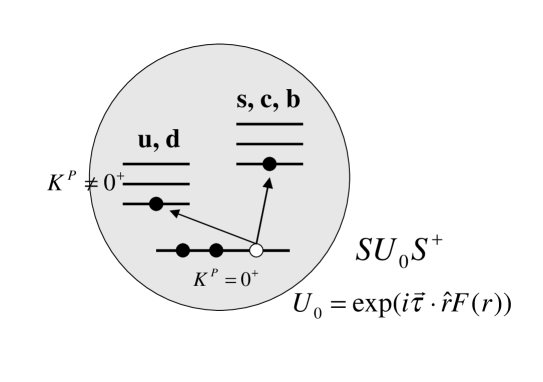
Figure 3: Two classes of excitation spectrum described by Berry potentials: Class A for excitations within up and down quark space; Class B for excitations involving heavy quark $Q=s,c,b\cdots$

To expose the physics behind the second term of (I.260) which is the principal element of our argument, we expand the fermionic fields in the complete set of states $\psi_{KM}$ with energies $\epsilon_{K}$ in the unrotating bag corresponding to the action $S_{S=1}$ in (I.260), and $M$ labels $2K+1$ projections of the grand spin $K$. Generically,

$$\psi(t,x)=\sum_{K,M}c_{KM}(t)\psi_{KM}(x)$$ (I.261)

where the $c$’s are Grassmannians, so that

$$S=\sum_{KM}\int dt\,\,c^{{\dagger}}_{KM}(i\partial_{t}-\epsilon_{K})c_{KM}+\sum_{KMK^{{}^{\prime}}N}\int dt\,\,c^{{\dagger}}_{KM}A^{KK^{{}^{\prime}}}_{MN}c_{K^{{}^{\prime}}N}$$ (I.262)

where

$$A_{MN}^{KK^{{}^{\prime}}}=\int_{V}d^{3}x\,\psi^{{\dagger}}_{KM}S^{{\dagger}}i\partial_{t}S\psi_{K^{{}^{\prime}}N}\,.$$ (I.263)

No approximation has been made up to this point. If the $A$ of (I.263) were defined in the whole $K$ space, then $A$ takes the form of a pure gauge and the field strength tensor would be identically zero . However we are forced to truncate the space. As in the preceding cases, we can use now the adiabatic approximation and neglect the off-diagonal terms in $K$, i.e., ignore the effect of adiabatic rotations that can cause the jumps between the energy levels of the fast quarks. Still, for every $K\neq 0$ the adiabatic rotation mixes $2K+1$ degenerate levels corresponding to particular fast eigenenergy $\epsilon_{K}$. In this form we clearly see that the rotation induces a hierarchy of Berry potentials in each K-band, on the generic form identical to Eq.(I.207). This field is truly a gauge field. Indeed, any local rotation of the $\psi_{KM}\rightarrow D^{K}_{MN}\psi_{KN}$ where $D^{K}$ is a $2K+1$ dimensional matrix spanning the representation of rotation in the $K$-space, can be compensated by a gauge transformation of the Berry potential

$$A^{K}\rightarrow D^{K}(\partial_{t}+A^{K})D^{K{\dagger}}$$ (I.264)

leaving $S_{S}$ invariant. A potential which has this transformation property is called “invariant gauge potential” [42].

The structure of the Berry potential depends on the choice of the parameterization of the isorotation $S$ (which is related to the gauge freedom). For the parameterization $S=a_{4}+i\vec{a}\cdot\vec{\tau}$ with the unitary constraint $a\cdot a=1$ (unitary gauge), we have

$$A^{K}=T_{K}^{a}\,A_{K}^{a}=T_{K}^{a}\,\left(\,g_{K}\,\,\frac{\eta_{\mu\nu}^{a}\,a_{\mu}da_{\nu}}{1+a^{2}}\right)$$ (I.265)

where $\eta$ is the ’t Hooft symbol and $g_{K}$ the induced coupling to be specified below. The $T$’s refer to the K-representation of $SU(2)$, the group of isorotations. In the unitary gauge the Berry potential has the algebraic structure of a unit size instanton in isospace, i.e, the space of the slow variables. It is not the Yang-Mills instanton, since the above configuration is not self-dual due to the unitary gauge constraint. This configuration is a non-abelian generalization of the monopole-like solution present in the diatomic molecular case.

To make our analogy more quantitative, let us refer to the Grassmannians $c$ in the valence states by $\alpha$’s and those in the Dirac sea by $\beta$’s. Clearly (I.262) can be trivially rewritten in the form

$$S = \sum_{KMN}\int dt\,\,{\alpha}^{{\dagger}}_{KM}\left[(i\partial_{t}-\epsilon_{K}){\bf 1}_{MN}+(A^{K})_{MN}\,\right]\alpha_{KN}$$ (I.266)

$$+ \sum_{KMN}\int dt\,\,{\beta}^{{\dagger}}_{KM}\left[(i\partial_{t}-\epsilon_{K}){\bf 1}_{MN}+(A^{K})_{MN}\,\right]\beta_{KN}\,.$$

Integrating over the Dirac sea in the presence of valence quarks yields the effective action

$$S= \sum_{KMN}\int dt\,\,{\alpha}^{{\dagger}}_{KM}\left[(i\partial_{t}-\epsilon_{K}){\bf 1}_{MN}+(A^{K})_{MN}\,\right]\alpha_{KN}$$

$$+ i{\rm Tr}\,{\rm ln}\,\left((i\partial_{t}-\epsilon_{K}){\bf 1}_{MN}+(A^{K})_{MN}\,\right)$$ (I.267)

where the Trace is over the Dirac sea states. The latter can be Taylor expanded in the isospin velocities $\dot{a}_{\mu}$ in the adiabatic limit,

$$i{\rm Tr}\,{\rm ln}\,((i\partial_{t}-\epsilon_{k}){\bf 1}_{MN}-({\cal A}_{\mu}^{K})_{MN}\dot{a}_{\mu})=\int\,dt\,\frac{{{\cal I}}_{q}}{2}\dot{a}_{\mu}\dot{a}_{\mu}+\cdots$$ (I.268)

where ${{\cal I}}_{q}$ is the moment of inertia contributed by the quark sector. We have exposed the velocity dependence by rewriting the form $A^{K}_{MN}=({\cal A}_{\mu}^{K})_{MN}\dot{a}_{\mu}$. Linear terms in the velocity are absent since the Berry phases in the sea cancel pairwise in the SU(2) isospin case under consideration. (For SU(3) they do not and are at the origin of the WZW term.) The ellipsis in (I.268) refers to higher derivative terms. We should point out that Eq.(I.268) includes implicitly the valence quark effect, because the levels of the Dirac sea are modified due to the presence of the valence quarks.

To clarify the general motivation for studying the excited states in terms of Berry phases, let us consider the case of the bag containing one valence quark in the $K=1$ state. The action for the adiabatic motion of this quark is obtained from the above formulae and yields (sum over repeated indices is understood)

$$S=\int dt\,\,[i{\alpha}^{{\dagger}}_{1M}\dot{\alpha}_{1M}-\epsilon_{1}\alpha^{{\dagger}}_{1M}\alpha_{1M}+\frac{1}{2}{{\cal I}}_{q}\dot{a}_{\mu}\dot{a}_{\mu}+\dot{a}_{\mu}({\cal A}_{\mu}^{1})_{MN}\alpha_{1M}^{{\dagger}}\alpha_{1N}]\,.$$ (I.269)

As we will see below, when canonically quantized, the generic structure of the resulting Hamiltonian is identical to (I.251). This illustrates the universal character of the Berry phases.

2.3.2 Excitation spectrum

To quantize the system, we note that (I.269) describes the motion of a particle with nonabelian charges coupled to an instanton-like gauge field on $S^{3}$. Since $S^{3}$ is isomorphic to the group manifold of $SU(2)$, it is convenient to use the left or right Maurer-Cartan forms as a basis for the vielbeins (one-form notation understood)

$$S^{\dagger}idS=-\omega_{a}\tau_{a}=-v_{a}^{c}(\theta)d\theta^{c}\tau^{a}$$ (I.270)

where we expressed the “velocity” forms $\omega$ in the basis of the vielbeins $v_{a}^{c}$, and $\theta$ denotes some arbitrary parametrization of the $SU(2)$, e.g. Euler angles. In terms of vielbeins, the induced Berry potential simplifies to

$${\cal A}^{c}=g_{K}A_{K}^{c}=-\,g_{K}\,v_{a}^{c}(\theta)T^{a}$$ (I.271)

where $T$ are generators of the induced Berry structure in the $K$ representation and $g_{K}$ is the corresponding charge [30], the explicit form of which is not needed.

Note that we could have equally well used the right-invariant Maurer-Cartan form instead of the left-invariant Maurer-Cartan form (I.270). The field strength can be written in terms of $A$ defined in Eq.(I.271)

$${\cal F}_{K}=dA_{K}-ig_{K}A_{K}\wedge A_{K}=-(1-g_{K}/2)\epsilon^{mij}T_{K}^{m}\,v^{i}\wedge v^{j}.$$ (I.272)

${\cal F}_{K}$ vanishes for $g_{K}=2$, $i.e.$ the Berry potential becomes a pure gauge. The vielbeins, and hence $A$ and ${\cal F}$ are frame-dependent, but to quantize the system no specific choice of framing is needed. The canonical momenta are $p_{a}={\partial L}/{\partial\dot{\theta}_{a}}$. Our system lives on $S^{3}$ and is invariant under $SO(4)\sim SU(2)\times SU(2)$. Right and left generators are defined as

$$R_{a} = u_{a}^{c}\,p_{c}$$

$$L_{a} = D_{ab}(S)\,R_{b}$$ (I.273)

where $u^{a}_{i}\,v^{i}_{c}=\delta_{c}^{a}$ and $D(S)$ spans the adjoint representation of $SU(2)$. Following the standard procedure we get our Hamiltonian in terms of the generators

$$H^{*}=\epsilon_{K}\,{\bf 1}+\frac{1}{8{\cal I}}\,\left(R_{j}-g_{K}\,T_{Kj}\right)\left(R_{j}-g_{K}\,T_{Kj}\right).$$ (I.274)

Here ${{\cal I}}$ is the total moment of inertia, the sum of the quark contribution and the mesonic contribution. As a result the Hamiltonian for a single excited quark takes the simple form

$$H^{*}=\epsilon_{1}{\bf 1}+\frac{1}{8{\cal I}}\left(\vec{R}^{2}-2g_{K}\vec{R}\cdot\vec{T}_{K}+g_{K}^{2}\vec{T}_{K}^{2}\right)$$ (I.275)

The spectrum can be readily constructed if we notice that (I.275) can be rewritten solely in terms of the independent Casimirs

$$H^{*}=\epsilon_{K}{\bf 1}+\frac{1}{2{\cal I}}\left[+\frac{g_{K}}{2}\vec{J}_{K}^{2}+(1-\frac{g_{K}}{2})\vec{I}^{2}-\frac{g_{K}}{2}(1-\frac{g_{K}}{2})\vec{T}^{2}\right]$$ (I.276)

where $\vec{J}_{K}={\vec{R}}/{2}-\vec{T}_{K}$ and $\vec{I}=\vec{L}/2$. We recall that $\vec{L}^{2}=\vec{R}^{2}$ on $S^{3}$. The set $J_{K}^{2}$, $I^{2}$, $J_{K3}$ and $I_{3}$ form a complete set of independent generators that commute with $H^{*}$. They can be used to span the Hilbert space of a single quark in the $K$ band. We will identify $J_{K}$ with the angular momentum and $I$ with the isospin.

The spectrum associated with (I.276) will be analyzed both in the light-quark and heavy-quark sectors when we have discussed the skyrmion structure. Let us briefly mention here that in the light-quark system, the limit $g_{K}=0$ for which the induced angular momentum $-\vec{T}_{K}$ decouples from the system (which would correspond to $(1-\kappa)=0$ in the diatomic molecule) is never reached. Neither is the abelian limit that will be attained for $g_{K}=2$ physically relevant. On the other hand, as we will explicitly show in Lecture II, the decoupling limit is attained in heavy-quark baryons because of the presence of heavy-quark symmetry that is present in QCD in the limit the heavy-quark mass becomes infinite.

Part II Skyrmions

[Updating remark]

[No significant development has been made in the skyrmion description of the ground state and excited baryons since the ELAF93 lecture although there have been some quantitative improvements in comparing with experiments. Some major developments have been made, however, in the mathematical studies of multi-baryon systems, namely, nuclei and nuclear matter. Some of this development will be commented on in the later section. There have been more excitements on the role of skyrmions in condensed matter physics, in connection with fractional quantized Hall effects, Bose-Einstein condensation etc. but this topic is outside of the scope of this note.]

1 Ground-State Baryons

In this lecture, we shrink the bag to a point using the Cheshire Cat strategy and consider it to be a gauge-fixed version of the chiral bag. We assume that the resulting system is a skyrmion [43] and describes the physics of the baryons. First we describe the ground-state systems, the nucleon and the $\Delta$. Excitations both in the light-flavor sector and in the heavy-flavor sector will then be discussed in terms of Berry potentials.

1.1 Large $N_{c}$ Consideration

The notion of large number of colors ($N_{c}$) plays an essential role in deriving or guessing effective Lagrangians of QCD applicable at low energy in terms of finite number of long wavelength meson excitations. We have used it (albeit implicitly) for the Cheshire Cat mechanism in four dimensions. The outcome of large $N_{c}$ considerations is a Lagrangian that contains weakly coupled meson fields only. If such a Lagrangian is the entire content of QCD at low energy, then where are the ground-state baryons? We have shown in the previous section that even when only Goldstone bosons are excited, there is a certain sense in which baryons could emerge through the approximate CCP. Here we discuss how in large-$N_{c}$ QCD baryons can emerge as solitons in mesonic effective theories. Note that the CCP argument did not rely on large $N_{c}$ explicitly. But the argument based on large $N_{c}$ implies that the CCP is a better approximation the larger the $N_{c}$.

That baryons must appear as solitons in meson field theory [44] is plausible but not fully established. The reason is that even in the limit $N_{c}=\infty$, the exact solution of QCD is not available. In any event, in the large $N_{c}$ limit, QCD is a weakly interacting meson field theory, with the meson mass going as $O(1)$ in $1/N_{c}$ and the $n$-Goldstone boson function going as $\sim N_{c}^{\lambda}$, $\lambda=(2-n)/2$. The meson scattering amplitude is described by the tree graphs of this effective Lagrangian with the coupling constant proportional to $1/\sqrt{N_{c}}$, so goes to zero as $N_{c}$ tends to infinity. Now this theory has no fermions and hence no explicit baryons. In quark picture, one needs $N_{c}$ quarks to make up a baryon, so the mass of a baryon must go like

$$m_{B}\sim N_{c}=\frac{1}{1/N_{c}}.$$ (II.1)

Such an object can occur from mesons only if there is a soliton in the meson field configuration. Such a configuration is known to exist in less than four dimensions and well understood. In four dimensions, we have the magnetic monopole which has not yet been seen experimentally. The soliton mass in weakly coupled meson field theory does indeed go like $1/\alpha$ where $\alpha$ is the coupling constant of the meson fields. Thus it must be that a baryon in QCD is a soliton with a large mass $\sim N_{c}$ with a size of $O(1)$. In the same vein, a nucleus made of $A$ nucleons must be a soliton of mass $\sim AN_{c}$ of the same mesonic Lagrangian.

In treating baryons as solitons, the basic assumption is that the bulk of baryon physics is dictated by the leading $N_{c}$ contributions and next $1/N_{c}$ corrections are in some systematic fashion calculable. It is not obvious that such corrections are necessarily small. For instance, nuclear binding is of $O(1/N_{c})$ and hence nuclei exist in the subleading order. So how useful is the concept of nucleons and nuclei as solitons? This is the question addressed below.

1.2 Soliton

1.2.1 Stability of the soliton

The large $N_{c}$ consideration suggests that baryons, if at all, can only arise from mesonic effective theories as solitons. Let us first see whether a stable soliton can indeed be obtained from simple meson Lagrangians.

The longest wavelength chiral Lagrangian is the leading nonlinear $\sigma$-model Lagrangian

$${{\cal L}}_{2}=\frac{f^{2}}{4}{\mbox{Tr}}(\partial_{\mu}U\partial^{\mu}U^{\dagger}).$$ (II.2)

Does this Lagrangian by itself give a stable soliton? One can answer this question quite simply.

Before proceeding to answer this question, we have to introduce a basic notion of a soliton in the way that we are using here . (The notion of soliton as used in particle and nuclear physics is different from other fields where the term soliton is applied to localized solutions which maintain their form even in scattering process.) Since we are going to shrink the bag to a point, we will consider only topological solitons, not the nontopological variety one finds in the literature. The topology involves space of fields of $U$. A sufficient condition for the existence of a soliton is that

$$U(\vec{x},t)\rightarrow 1\ \ \ \ {\rm as}\ \ |\vec{x}|=r\rightarrow\infty$$ (II.3)

with the rate of approach of $U$ to $1$ sufficiently fast so that the energy is finite, say, $E<\infty$. Consider the usual hedgehog ansatz made by Skyrme a long time ago [43]

$$U_{0}(\vec{x})=e^{i\hat{x}\cdot\vec{\tau}F(r)}.$$ (II.4)

Then the static energy functional is

$$E = 2\pi f^{2}\int_{\epsilon}^{\infty}r^{2}dr\left[(dF/dr)^{2}+\frac{2}{r^{2}}\sin^{2}F\right]$$ (II.5)

$$= 2\epsilon\pi f^{2}\int_{1}^{\infty}y^{2}dy\left[(dF/dy)^{2}+\frac{2}{y^{2}}\sin^{2}F\right]$$

where the second equality is obtained with the change of variable $y\equiv r/\epsilon$. We have put $\epsilon$ for the lower limit for the reason that will be apparent soon. If we let $\epsilon=0$, then the energy of the system is zero. Since the integral is positive definite, this is the lowest energy. Now $f$ has a dimension of mass and since the only other scale parameter possible is the size of the system ($R$), the energy must be proportional to $f^{2}R$ and hence the lowest energy solution corresponds to the zero size, namely, a collapsed system. This is the well-known result of “Hobart-Derrick theorem” [45]. Since there is no known massless point-like hadron with fermion quantum number, this must be an artifact of the defects of the theory.

There is one simple way [46] to avoid the Hobart-Derrick collapse without introducing any further terms in the Lagrangian or any other degrees of freedom, which is interesting and in a way, physically relevant. It is to simulate short-distance physics by “drilling” a hole into the skyrmion or equivalently by taking a nonzero $\epsilon$ in the energy functional (II.5). This is not as academic an issue as it seems since a hole of that type arises naturally in the chiral bag model discussed before. Let us for the moment ignore what is inside that hole and see what that hole does to the system. Since the detail of the analysis that establishes the existence of a stable soliton for $\epsilon\neq 0$ is not very relevant to us as there is a natural way of assuring a stable system using a realistic quark bag, it suffices to just summarize what transpires from the analysis: For any nonzero value of $\epsilon$, there is always a solution which is classically stable in the sense of escaping the Hobart-Derrick theorem and is stable against small fluctuation $\eta$ of the solution $F$

$$F(y)\rightarrow F(y)+\eta(y).$$ (II.6)

Since the system definitely collapses for $\epsilon=0$, it is clearly a singular point. This singular behavior is probably related to the presence or absence of a topological quantum number in the chiral bag [47]. Indeed a chiral bag can be shrunk to a point without losing its topological structure as long as a proper chiral boundary condition is imposed. Without the boundary condition, the topological quantum number is not conserved and the bag decays into a vacuum. Thus a nontrivial topological structure requires a finite $\epsilon$ to allow the boundary condition to be imposed at the bag boundary and if the bag is shrunk, then at the center. A relevant physical question is how to determine $\epsilon$. One practical approach suggested by Balakrishna et al [46] is to elevate it to a quantum variable whose expectation value is related to the “bag radius.” From this point of view, a bag is a necessary physical ingredient. On the other hand, although this is highly suggestive, the discussion on the Cheshire cat phenomenon given above clearly indicates that the picture of replacing a quark bag by a quantized cut-off variable can only be an academic one.

Another way of stabilizing the system for $\epsilon=0$ might be to introduce quantum fluctuations before solving for the minimum configuration. It is plausible that quantum effects could stabilize the system by themselves just as the collapse of the S-wave state of the classical hydrogen atom can be prevented by quantum fluctuations. It turns out that just quantizing a few collective degrees of freedom such as scale variable does not work without a certain “confinement” artifact of the sort mentioned above. So far nobody has been able to stabilize the skyrmion of (II.5) with $\epsilon=0$ in a fully convincing way. This of course does not mean that such a scheme is ruled out. There are many other collective variables than the scale variable to quantize and it is possible that by suitable quantization of appropriate variables, the system could be stabilized. We want to stress here however that all these are really academic issues. We are working with effective Lagrangians that are supposed to model QCD. Hence there are many other degrees of freedom in nature, be they in quark variables as in the chiral bag or in meson variables such as the strong vector mesons. We saw above that a quark-bag does trivially avoid the Hobart-Derrick collapse. As one eliminates the quark bag, higher derivative terms in the chiral field arise through various induced gauge fields as discussed above, among which we can have the quartic term

$$\frac{1}{32g^{2}}{\mbox{Tr}}[U^{\dagger}\partial_{\mu}U,U^{\dagger}\partial_{\nu}U]^{2}$$ (II.7)

the so-called “Skyrme quartic term” which Skyrme introduced (in a somewhat ad hoc way) to stabilize the soliton. We know now that such a term can arise in some particular way from the $\rho$ meson when the latter is integrated out. We can readily verify that this term is enough to stabilize the soliton. To see this, let us scale $U(x)\rightarrow U(\lambda x)$. Then the energy of the system changes

$$E_{\lambda}=\lambda^{2-d}E_{(2)}+\lambda^{4-d}E_{(4)}$$ (II.8)

where the first term is the contribution from the quadratic term and the second from the quartic term, with subscripts labelling them appropriately and $d$ is the space dimension (equal to 3 in nature). The minimum condition implies

$$dE_{\lambda}/d\lambda=0\rightarrow E_{(2)}/E_{(4)}=-(d-4)/(d-2)$$ (II.9)

and the stability implies

$$d^{2}E_{\lambda}/d\lambda^{2}>0\rightarrow 2(d-2)E_{(2)}>0.$$ (II.10)

Thus for stability, we need $d>2$ which is fine with $d=3$ for which we have $E_{(2)}=E_{(4)}$, the virial theorem. What this implies is then that once one has more massive strong interaction degrees of freedom, the stability issue is no longer a real issue. Indeed there have been considerable controversy as to what vector mesons stabilize the soliton, in particular, the question as to whether the $\rho$ meson can do the job by itself. It is now understood that while the Skyrme quartic term which can be traced to the $\rho$ meson in origin stabilizes the system, the finite-range $\rho$ meson cannot and it is instead the $\omega$ meson which plays the role of stabilization. There is no lack of candidates for the role if some do not do the job. Our attitude will be that the skyrmion is safe from the Hobart-Derrick collapse and so we can simply proceed to the real stuff, namely physics of the skyrmion. Those readers who want to know more about the technicality are referred to the literature.

1.2.2 Structure of the soliton

The original Skyrme model captures the essence of the soliton structure, so we will focus on the Lagrangian

$${{\cal L}}_{sk}=\frac{f^{2}}{4}{\mbox{Tr}}(\partial_{\mu}U\partial^{\mu}U^{\dagger})+\frac{1}{32g^{2}}{\mbox{Tr}}[U^{\dagger}\partial_{\mu}U,U^{\dagger}\partial_{\nu}U]^{2}.$$ (II.11)

A quantitatively more precise prediction can be made with a Lagrangian that contains the strong vector mesons in consistency with hidden gauge symmetry [48]. If the vector mesons are introduced disregarding HGS, one has to make sure that the chiral counting comes out correctly, which is not always transparent but the physics is not qualitatively modified by it. The static energy of the skyrmion given by (II.11) reads

$$E=\int d^{3}x\left\{-\frac{f^{2}}{4}{\mbox{Tr}}L_{i}^{2}-\frac{1}{32g^{2}}{\mbox{Tr}}[L_{i},L_{j}]^{2}\right\}$$ (II.12)

with $L_{i}=U^{\dagger}\partial_{i}U$. It is convenient to scale the length by $1/gf$ by setting $x\rightarrow(1/gf)x$ and give the energy in units of $f/2g$. In these units, the energy reads

$$E=\int d^{3}x\left\{-\frac{1}{2}{\mbox{Tr}}L_{i}^{2}-\frac{1}{16}{\mbox{Tr}}[L_{i},L_{j}]^{2}\right\}.$$ (II.13)

One can rewrite this

$$E = \int d^{3}x\frac{-1}{2}{\mbox{Tr}}\left\{L_{i}\pm\frac{1}{4}\epsilon_{ijk}[L_{j},L_{k}]\right\}^{2}$$ (II.14)

$$\pm 12\pi^{2}\int d^{3}x\frac{1}{24\pi^{2}}\epsilon_{ijk}{\mbox{Tr}}(L_{i}L_{j}L_{k}).$$

The first term is non-negative and the second integral measures the winding number which can be identified with the baryon number $B$

$$B=\frac{1}{24\pi^{2}}\int d^{3}x\epsilon_{ijk}{\mbox{Tr}}(L_{i}L_{j}L_{k})$$ (II.15)

and so we have the topological bound on the energy

$$E\geq 12\pi^{2}|B|.$$ (II.16)

This bound is known as Faddeev bound [49]. This bound would be saturated if we had the equality

$$L_{i}+\frac{1}{4}\epsilon_{ijk}[L_{j},L_{k}]=0.$$ (II.17)

But it turns out that the only solution to this equation is the trivial one, namely, $U=constant$ and so $L_{i}=0$ [50]. It turns out also that in curved space, this bound can actually be satisfied and plays an interesting role in connection with chiral symmetry restoration.

To proceed further, we shall now take an ansatz for the chiral field $U$. In particular we assume the hedgehog form

$$U({\bf x})=e^{iF(r)\hat{x}\cdot{\bf\tau}}.$$ (II.18)

With this, the energy (II.13) is

$$E = 4\pi\int_{0}^{\infty}\,dr\left\{r^{2}[(dF/dr)^{2}+2r^{-2}\sin^{2}F]+\sin^{2}F[r^{-2}\sin^{2}F+2(dF/dr)^{2}]\right\}$$ (II.19)

$$= 4\pi\int_{0}^{\infty}\,dr[r^{2}(dF/dr+r^{-2}\sin^{2}F)^{2}+2\sin^{2}F(dF/dr+1)^{2}]$$

$$-24\pi\int_{0}^{\infty}\,dr\sin^{2}F\frac{dF}{dr}.$$

For the energy to be finite, $U$, (II.18), must approach a constant at infinity which can be chosen to be the unit matrix. This means that the space is compactified to three-sphere ($S^{3}$) and $U$ represents a map from $S^{3}$ to to $SU(2)$ which is topologically $S^{3}$, the winding number of which was given by the right-hand side of (II.15). The implication of this on Eq. (II.19) is that since the “profile function” $F$ at the origin and at infinity must be an integral multiple of $\pi$, the second term of (II.19) must correspond to $12\pi[F(0)-F(\infty)]=12\pi^{2}B$, the Faddeev bound. As mentioned above, the first integral of (II.19) cannot vanish for a nontrivial $U$ in flat space, so the energy is always greater than $12\pi^{2}B$.

Minimizing the energy with respect to the profile function $F$ gives us the classical equation of motion. The exact solution with appropriate boundary conditions at the origin and at infinity is known [51, 52] but only numerically. For the present qualitative discussion, we do not need a precise form for $F$. Indeed one can infer a simple analytic form by the following argument[50]. First of all, it turns out numerically that the the first integral in (II.19) is small so that the soliton energy is only slightly greater than the Faddeev bound. The equation of motion shows that $F(r)$ goes like $B\pi-\alpha(r/r_{0})$ as $r\rightarrow 0$ and like $\beta(r_{0}/r)^{2}$ as $r\rightarrow\infty$ with some constant $r_{0}$. Let us therefore take the form for $B=1$

$$F = \pi-\alpha(r/r_{0}),\ \ \ \ r\leq r_{0},$$ (II.20)

$$= \beta(r_{0}/r)^{2},\ \ \ \ \ \ \ \ r\geq r_{0}.$$ (II.21)

Demanding the continuity of $F$ and its first derivative with respect to $r$ at $r=r_{0}$, one determines

$$\alpha=2\pi/3,\ \ \ \ \beta=\pi/3.$$ (II.22)

Substituting (II.21) with (II.22) into (II.19), one finds

$$E\approx 4\pi(4.76r_{0}+7.55/r_{0})$$ (II.23)

where the coefficients of $r_{0}$ and $1/r_{0}$ are estimated numerically. Minimizing with respect to $r_{0}$, one gets $r_{0}=1.26$ (in units of $(gf)^{-1}$) and $E=151$ (in units of $f/2g$) which is 1.03 times the exact energy evaluated numerically. The ansatz (II.21) is numerically close to the exact numerical solution. 

It is mentioned above that the true energy of the soliton is only slightly greater than the Faddeev bound $12\pi^{2}$. Numerically it turns out to be about 23 % above. An interesting question is: When can the Faddeev bound be saturated? As stated, this can never happen in flat space, which is the case in nature since the space we are dealing with is $R^{3}$ or $S^{3}(\infty)$, the three-sphere with an infinite radius. Consider instead the space $S^{3}(L)$ with $L$ finite. Let its (inverse) metric be $g^{ij}$ and denote the dreibein $e_{m}^{j}$ so that

$$g^{ij}=e^{i}_{m}e^{j}_{m}.$$ (II.24)

If we define

$$X_{m}\equiv e^{i}_{m}\partial_{i}UU^{\dagger}$$ (II.25)

then the static energy of the system is (for $n_{B}=1$)

$$E=\int d^{3}x\sqrt{g}[-\frac{1}{2}(X_{m}+\frac{1}{4}\epsilon_{mnp}[X_{n},X_{p}])^{2}]+12\pi^{2}.$$ (II.26)

The topological term, $12\pi^{2}$, is independent of the metric as expected. Now the bound is saturated provided

$$X_{m}+\frac{1}{4}\epsilon_{mnp}[X_{i},X_{j}]=0.$$ (II.27)

When the space is flat (i.e, $L=\infty$), this equation reduces to Eq. (II.17) which has no nontrivial solution as already mentioned above. In curved space, however, it has a solution when $L=1$. This is an identity map, inducing no distortion and corresponds to isometry. One can perhaps associate this particular solution with a state of symmetry different from the spontaneously broken chiral symmetry for which the bound can never be satisfied.

1.2.3 Quantization of the soliton

To give a physical meaning, the soliton has to be quantized. As it is, the hedgehog solution is not invariant under separate rotation in configuration space or in isospace. It is invariant under the simultaneous rotation of the two, with the conserved quantum number being the “grand spin” which is the vector sum of the spin and the isospin

$$\vec{K}=\vec{J}+\vec{I}.$$ (II.28)

The hedgehog configuration breaks the rotational symmetry as mentioned, as a consequence of which there are three zero modes corresponding to the triplet of the isospin direction. For $S\in SU(2)$, the equation of motion of the hedgehog is invariant under the transformation

$$U(\vec{x})\rightarrow SU(\vec{x})S^{\dagger}$$ (II.29)

so the states obtained by rotating the hedgehog are degenerate with the unrotated hedgehog. To restore the symmetry, one has then to elevate $S$ to a quantum variable by endowing it a time dependence and quantize the zero modes. This is essentially equivalent to rotating the hedgehog. It is also equivalent to projecting out good angular momentum and isospin states. Note that in discussing induced gauge fields above, we have already encountered the notion of an adiabatic rotation. Since this rotation leads to next order in $1/N_{c}$ in $N_{c}$ counting in physical quantities, we are implicitly making the adiabatic approximation.

Substituting $U(\vec{x},t)=S^{\dagger}(t)U(\vec{x})S(t)$ into the Skyrme Lagrangian (II.11), we get

$$L_{sk}=-{\cal M}+{\cal I}{\mbox{Tr}}(\dot{S}\dot{S}^{\dagger})$$ (II.30)

with

$${\cal I}=\frac{2\pi}{3}\frac{1}{g^{3}f}\int_{0}^{\infty}\,s^{2}ds\sin^{2}F[1+4{F^{\prime}}^{2}+4\frac{\sin^{2}F}{s^{2}}]$$ (II.31)

where $s=fgr$ is the dimensionless radial coordinate and ${\cal M}=E$, the soliton energy. Note that in terms of $N_{c}$, both ${\cal M}$ and ${\cal I}$ are of order $N_{c}$ while $\dot{S}$ is of order $1/N_{c}$. The theory can now be quantized canonically in a standard way. To do so, introduce the collective coordinates $(a_{0},\vec{a})$ by

$$S=a_{0}+i\vec{\tau}\cdot\vec{a}$$ (II.32)

with

$$S^{\dagger}S=1=a_{0}^{2}+\vec{a}^{2}.$$ (II.33)

The momentum conjugate to $a_{k}$ is

$$\pi_{k}=\frac{\partial L_{k}}{\partial\dot{a}_{k}}=4{\cal I}\dot{a}_{k}.$$ (II.34)

The Hamiltonian is

$$H=\sum_{k=0}^{3}\pi_{k}\dot{a}_{k}-L_{sk}={\cal M}+\frac{1}{8{\cal I}}\sum_{k=0}^{3}\pi_{k}^{2}.$$ (II.35)

Quantization is effected by taking $\pi_{k}=-i(\partial/\partial a_{k})$; thus

$$H={\cal M}+\frac{1}{8{\cal I}}\sum_{k=0}^{3}\left(-i\frac{\partial}{\partial a_{k}}\right)^{2}.$$ (II.36)

The second term is just the Laplacian on $S^{3}$ whose eigenstates are the Jacobi polynomials in $a$’s. Using the Noether method, the spin $J$ and isospin $I$ can be calculated

$$J_{k} = \frac{i}{2}\left(a_{k}\frac{\partial}{a_{0}}-a_{0}\frac{\partial}{\partial a_{k}}-\epsilon_{klm}a_{l}\frac{\partial}{\partial a_{m}}\right),$$ (II.37)

$$I_{k} = \frac{i}{2}\left(a_{0}\frac{\partial}{\partial a_{k}}-a_{k}\frac{\partial}{\partial a_{0}}-\epsilon_{klm}a_{l}\frac{\partial}{\partial a_{m}}\right)$$ (II.38)

with

$$\vec{J}^{2}=\vec{I}^{2}=\frac{1}{4}\sum_{k=0}^{3}\left(-\frac{\partial^{2}}{\partial a_{k}^{2}}\right).$$ (II.39)

Therefore the Hamiltonian describes a spherical top

$$H={\cal M}+\frac{1}{2{\cal I}}\vec{J}^{2}.$$ (II.40)

The energy eigenstates of this Hamiltonian can be explicitly constructed as polynomials in $a$’s. Whether they are even or odd polynomials depends upon whether the object satisfies bosonic or fermionic statistics. A detailed discussion on this matter will be given in the next subsection. If one considers fermions, then for the ground state $J=I=1/2$ and its wavefunction will then be a monomial in $a$’s. Specifically[52],

$$|p\uparrow\rangle=\frac{1}{\pi}(a_{1}+ia_{2}),\ \ \ \ |p\downarrow\rangle=-\frac{i}{\pi}(a_{0}-ia_{3}),$$ (II.41)

$$|n\uparrow\rangle=\frac{1}{\pi}(a_{0}+ia_{3}),\ \ \ \ |n\downarrow\rangle=-\frac{1}{\pi}(a_{1}-ia_{2}).$$ (II.42)

These can be identified with the physical proton with spin up or down and neutron with spin up or down. A similar construction can be made for the excited states with $J=I=3/2$ etc. A more general construction will be given later when we include the strangeness in the scheme.

1.3 Light-Quark Skyrmions

We have thus far motivated within the Cheshire cat picture that the object we have, namely the skyrmion, is a baryon. In what follows, we will supply further evidences that we are indeed dealing with what amounts to baryons expected in QCD. We will start with phenomenological aspects with $SU(2)$ skyrmions and later more mathematical aspects associated with the WZW term.

Some people have difficulty accepting the skyrmion as a bona-fide baryon consistent with QCD. They ask where the quark-gluon imprints are in the skyrmion description. They even attempt to find in skyrmions what should be there in QCD. In other words, their suspicion is that the skyrmion “misses” something basic of QCD. Throughout what follows, we will argue that this attitude is unfounded.

1.3.1 $SU(2)$ skyrmions

Masses

Let us assume that for $N_{c}$ odd, we have a fermion and when quantized as sketched above, it is a baryon. For $N_{c}=3$, we have two states $J=I=1/2$ and $J=I=3/2$. The first is the nucleon, the ground state and the second the excited state $\Delta$. In terms of $N_{c}$, their masses are of the form

$$M_{J}=M_{1}+M_{0}+M^{J}_{-1}+O(N_{c}^{-2})$$ (II.43)

where the subscript stands for $n$ in $N_{c}^{n}$. The $O(N_{c})$ term corresponds to the soliton mass ${\cal M}$ of Eq. (II.40) and the $O(N_{c}^{-1})$ to the “hyperfine structure” term, i.e, the second term of (II.40). The “fine structure” term $M_{0}$ has not yet been encountered. It is the first ($O(\hbar)$) quantum correction to the mass known as Casimir energy which describes the shift in energy of the vacuum produced by the presence of the soliton. Note that the two terms of $O(N_{c})$ and $O(1)$ define the ground state of the baryons and the dependence on quantum numbers appears at $O(1/N_{c})$. When heavy flavors are introduced, there will be an additional overall shift at $O(1)$ for each flavor. An important point is that the first two terms of (II.43) is common to all baryons, be they light-quark or heavy-quark baryons.

We will later present an argument that the term $M_{0}$ is attractive and can be of order of $\sim-0.5$ GeV. For the moment, let us treat it as a parameter independent of quantum numbers and estimate how much it could be from phenomenology. Let us consider the nucleon and $\Delta$. For definiteness, we will consider the Skyrme Lagrangian ${\cal L}_{sk}$ (II.11). There are two constants in the model, $f$ and $g$. We fix the constant $f$ to the pion decay constant $f_{\pi}=93$ MeV. The constant $g$ can be obtained from a more general Lagrangian containing HGS vector mesons but here we shall fix it from imposing that the $g_{A}$ of the neutron decay come out to be the experimental value 1.25 (see below how $g_{A}$ is calculated)[51]. The resulting value is $g\approx 4.76$. Restoring the energy unit $f/2g$, the soliton mass is

$$M_{1}={\cal M}=1.23\times 12\pi^{2}\left(\frac{f}{2g}\right)\approx 1423\ {\rm MeV}.$$ (II.44)

Similarly from (II.31), we get numerically

$${{\cal I}^{-1}}\approx 193\ {\rm{MeV}}.$$ (II.45)

We can now predict the mass difference between the $\Delta$ and $N$

$$\Delta M=\frac{3}{2}{\cal I}^{-1}\approx 290\ \rm{MeV}$$ (II.46)

to be compared with the experiment 296 MeV. The Casimir energy is a difficult quantity to calculate accurately and since our knowledge on it is quite uncertain, we cannot make a prediction for the absolute value of the ground state baryon (i.e, nucleon) mass. We can turn the procedure around and get some idea on the magnitude of the Casimir energy required for consistency with nature. Taking the nucleon mass formula with $J=1/2$, we have $M_{1}+\frac{3}{8}{\cal I}^{-1}\approx 1495$ MeV and hence

$$M_{0}\approx(940-1495)\ \rm{MeV}=-555\ \rm{MeV}.$$ (II.47)

This may look large but it is in the range expected theoretically as discussed below [53] and also consistent with the expectation based on the $N_{c}$ counting that

$$M_{1}>|M_{0}|>M_{-1}.$$ (II.48)

There is a caveat to this discussion which would modify the numerics somewhat. We have not taken into account the translational mode; the center-of-mass correction, which is of $O(N_{c}^{-1})$, should increase the centroid energy. Therefore the value of $M_{0}$ may even be higher in magnitude than (II.47).

Static properties

As an example of static quantities, consider the axial-vector coupling constant $g_{A}$. The nucleon matrix element of the axial current is

$$\langle N(p_{\prime})|A_{\mu}^{a}|N(p)\rangle=\bar{U}(p^{\prime})\frac{\tau^{a}}{2}\left[g_{A}(q^{2})\gamma_{\mu}\gamma_{5}+h_{A}(q^{2})q_{\mu}\gamma_{5}\right]U(p)$$ (II.49)

with $q_{\mu}=(p-p^{\prime})_{\mu}$ and $U(p)$ the Dirac spinor for the nucleon. We will continue working with the chiral limit, so the pseudoscalar form factor $h$ has the pion pole. Thus in the limit that $q_{\mu}\rightarrow 0$, we have

$$\lim_{q\rightarrow 0}\langle N(p^{\prime})|A_{i}^{a}|N(p)\rangle = \lim_{q\rightarrow 0}g_{A}(0)(\delta_{ij}-\hat{q}_{i}\hat{q}_{j})\langle N|\frac{\tau^{a}}{2}\sigma_{j}|N\rangle$$ (II.50)

$$= \frac{2}{3}g_{A}(0)\langle N|\frac{\tau^{a}}{2}\sigma_{i}|N\rangle$$

where we have expressed the matrix element in the nucleon rest frame. We now obtain the relevant matrix element in the present model. Using the axial current suitably “rotated”, we have

$$\int d\vec{x}A_{i}^{a}(\vec{x})=\frac{1}{2}\bar{g}{\mbox{Tr}}(\tau_{i}S^{\dagger}\tau_{a}S),$$ (II.51)

with

$$\bar{g}=\frac{2\pi}{3g^{2}}\int_{0}^{\infty}s^{2}ds\left(F^{\prime}+\frac{\sin 2F}{s}(1+4{F^{\prime}}^{2})+8F^{\prime}\frac{\sin^{2}F}{s^{2}}+4\frac{\sin^{2}F}{s^{3}}\sin 2F\right)$$ (II.52)

where we have used the dimensionless radial coordinate $s=(fg)r$. Note that given the profile function, $\bar{g}$ depends only on the constant $g$. The relevant matrix element is

$$\lim_{q\rightarrow 0}\int d\vec{x}e^{i{\vec{q}}\cdot{\vec{x}}}\langle N|A_{i}^{a}(\vec{x})|N\rangle=\frac{1}{2}\bar{g}\langle N|{\mbox{Tr}}(\tau_{i}S^{\dagger}\tau_{a}S)|N\rangle=\frac{2}{3}\bar{g}\langle N|\frac{\tau^{a}}{2}\sigma_{i}|N\rangle.$$ (II.53)

We are therefore led to identify

$$g_{A}(0)=\bar{g}.$$ (II.54)

Given $g_{A}$ from experiment, one can then determine the constant $g$ from this relation. The value $g\approx 4.76$ used in the mass formula was determined in this way.

Other static quantities like magnetic moments and various radii are calculated in a similar way and we will not go into details here, referring to standard review articles[55].

The Casimir energy

The calculation of the $O(N_{c}^{0})$ Casimir energy is in practice a very difficult affair although in principle it is a well-defined problem given an effective Lagrangian. The reason is that there are ultraviolet divergences that have to be cancelled by counter terms and since the effective theory is nonrenormalizable in the conventional sense, increasing number of counter terms intervene as one makes higher-order computations. In principle, given that the finite counter terms can be completely determined from experiments, the nonrenormalizability is not a serious obstacle to computing the Casimir contribution. The main problem is that chiral perturbation theory applicable in the Goldstone boson sector cannot be naively applied because of the baryon mass which is not small compared with the chiral scale $\Lambda_{\chi}\sim 4\pi f_{\pi}$. We will describe later how this problem is avoided in chiral expansion when baryon fields are explicitly introduced but it is not clear how to do so in the skyrmion structure.

The basic idea of computing the Casimir energy of $O(N_{c}^{0})$ is as follows: Let us consider specifically the Skyrme Lagrangian (II.11). The argument applies to any effective Lagrangian with more or less complications. Let $L_{\mu}\equiv i{\bf\tau}\cdot{\bf L}_{\mu}$. Then (II.11) takes the form

$${\cal L}_{sk}=\frac{f^{2}}{2}\left({\bf L}_{\mu}\cdot{\bf L}^{\mu}+\frac{1}{2\lambda^{2}}[({\bf L}_{\mu}\cdot{\bf L}^{\mu})^{2}-({\bf L}_{\mu}\cdot{\bf L}_{\nu})^{2}]\right)$$ (II.55)

with $\lambda=gf$. We denote by $\tilde{\bf L}_{\mu}$ the static solution of the Euler-Lagrange equation of motion

$$\partial^{\mu}\left(\tilde{L}_{\mu}^{a}+\frac{1}{\lambda^{2}}(\tilde{L}_{\mu}^{a}\tilde{\bf L}_{\nu}\cdot\tilde{\bf L}_{\nu}-\tilde{\bf L}_{\mu}\cdot\tilde{\bf L}_{\nu}\tilde{\bf L}_{\nu})\right)=0.$$ (II.56)

In terms of the chiral field $U$, the solution is of course the hedgehog we have seen above which we will denote by $U_{0}(\vec{x})$. We introduce fluctuation around $U_{0}$ by

$$U(x)=U_{0}e^{i{\bf\tau}\cdot{\bf\phi}}$$ (II.57)

and $L_{\mu}$ as

$${\bf L}_{\mu}=\tilde{\bf L}_{\mu}+\partial_{\mu}{\bf\phi}+\partial_{\mu}{\bf\phi}\wedge{\bf\phi}\cdots$$ (II.58)

Substitution of this expansion into (II.11) gives rise to a term zeroth order in ${\bf\phi}$ which is what we studied above for the nucleon and $\Delta$, a term quadratic in ${\bf\phi}$ and higher orders. There is no term linear in $\phi$ because its coefficient is just the equation of motion (II.56). To next to the leading order, the relevant Lagrangian is the quadratic term which takes the form

$$\Delta{\cal L}=\phi^{a}\left(H^{ab}+\cdots\right)\phi^{b},$$ (II.59)

$$H^{ab}=-\nabla_{\mu}^{2}\delta^{ab}-2\epsilon^{abc}\tilde{L}_{\mu}^{c}\nabla_{\mu}$$ (II.60)

where the ellipsis stands for the term coming from fluctuations around the Skyrme quartic term and higher derivative terms (and/or other matter fields in a generalized Lagrangian). Ignoring terms higher order in $\phi$’s, the effective potential $V^{eff}$ we wish to calculate is

$$e^{-i\int d^{4}xV^{eff}(\tilde{L})}=\int d[\phi]e^{i\int d^{4}x\Delta{\cal L}}.$$ (II.61)

The fluctuation contains the zero modes corresponding to three translational modes and three (isospin) rotational modes in addition to other “vibrational modes”. The three rotational modes were quantized to give rise to the correct quantum numbers of the baryons. Quantizing the translational zero modes is to restore the translational invariance to the system. We are here interested in the other modes which are orthogonal to these zero modes. This requires constraints or “gauge fixing”. Now doing the integral over the modes minus the six zero modes, we get formally

$$\int d^{4}xV^{eff}(\tilde{L})=-\frac{1}{2}{\mbox{Tr}}^{\prime}\ln(H+\cdots)$$ (II.62)

where the prime on trace means that zero energy modes of $H$ be omitted in the sum. This generates one-loop corrections to the effective potential. The $O(N_{c}^{0})$ Casimir energy, to one-loop order, is then given by

$$M_{0}=\frac{1}{T}\int d^{4}x\left(V^{eff}(\tilde{\bf L})-V^{eff}(0)\right)$$ (II.63)

where $T$ is the time interval. This can be evaluated by chiral perturbation theory. In doing so, one can ignore the quartic and higher derivative terms in (II.62) in the one-loop graphs since it leads to higher chiral order terms relative to the one-loop terms evaluated with the quadratic term $H$. In accordance with general strategy of chiral perturbation theory, the ultraviolet divergences are to be eliminated by counter terms involving four derivatives, with finite constants fixed by experiments. Those constants are available from analyses on $\pi\pi$ scattering. Using this strategy, several people have estimated this Casimir contribution to the nucleon mass. Because of the dubious validity in using the derivative expansion for skyrmions mentioned above, it is difficult to pin down the magnitude precisely: The magnitude will depend on the dynamical details of the Lagrangian and chiral loop corrections. The calculations, however, agree on its sign which is negative. Numerically it is found to range [53] from $\sim-200$ MeV to $\sim-1$ GeV. The recent more reliable calculations [56] give $\sim-500---600$ MeV, quite consistent with what seems to be needed for the ground-state baryon mass.

1.3.2 $SU(3)$ skyrmions: eight-fold way

We now study the system of three flavors u,d and s in the highly unrealistic situation where all three quarks are taken massless[54]. The idea that one can perhaps treat the three flavors on an equal footing, with the mass of the strange quark treated as a “small” perturbation turns out to be not good at all, but it provides a nice theoretical framework to study the role of the anomalous (Wess-Zumino) term which pervades even in realistic treatments given below. Putting the chiral field in $SU(3)$ space

$$U=e^{i\lambda^{a}\pi^{a}/f}$$ (II.64)

where $a$ runs over octet Goldstone bosons, we can generalize (II.11) to apply to $SU(3)$

$${\cal L}_{n}=-\frac{f^{2}}{4}{\mbox{Tr}}L_{\mu}L^{\mu}+\frac{1}{32g^{2}}{\mbox{Tr}}[L_{\mu},L_{\nu}]^{2}$$ (II.65)

and

$$S_{n}=\int d^{4}x{\cal L}_{n}$$ (II.66)

with $L_{\mu}$ defined with $U\in SU(3)$. While this Lagrangian was sufficient in $SU(2)$ space, it is not in $SU(3)$ space as mentioned before. Here we give a more physical argument for its “raison d’être” following Witten [20].

Consider two discrete symmetries $P_{1}$ and $P_{2}$

$$P_{1}: \ \ U(\vec{x},t)\rightarrow U(-\vec{x},t),$$ (II.67)

$$P_{2}: \ \ U(\vec{x},t)\rightarrow U^{\dagger}(\vec{x},t).$$ (II.68)

It is easy to see that (II.65) is invariant under both $P_{1}$ and $P_{2}$ and of course under parity

$$P=P_{1}P_{2}$$ (II.69)

which transforms

$$U(\vec{x},t)\rightarrow U^{\dagger}(-\vec{x},t).$$ (II.70)

QCD is of course invariant under parity but does not possess the symmetries $P_{1}$ and $P_{2}$ separately. For instance the well-known five pseudoscalar process $K^{+}K^{-}\rightarrow\pi^{+}\pi^{-}\pi^{0}$ is allowed by QCD but is not by the Lagrangian (II.65). Thus there must be an additional term that breaks $P_{1}$ and $P_{2}$ separately while preserving $P$. This information is encoded in the WZW term which we have encountered before in lower dimensions. In (3+1) dimensions, it is given by

$$S_{WZ}=-N_{c}\frac{i}{240\pi^{2}}\int_{D}d^{5}x\epsilon^{ijklm}{\mbox{Tr}}(\bar{L}_{i}\bar{L}_{j}\bar{L}_{k}\bar{L}_{l}\bar{L}_{m})$$ (II.71)

with $\bar{U}(\vec{x},t,s=0)=1$ and $\bar{U}(\vec{x},t,s=1)=U(\vec{x},t)$. Here $D$ is a five-dimensional disk whose boundary is the space time. The presence of the factor $N_{c}$ will be clarified later. It is easy to see that this has the right symmetry structure. It also carries other essential ingredients to render the CCP operative in baryon structure.

The action we will focus on is then the sum

$$S_{sk}=S_{n}+S_{WZ}.$$ (II.72)

As in the nonstrange hadrons, a marked improvement in quantitative agreement with experiments can be gained by introducing vector and axial-vector fields but the qualitative structure is not modified by those fields, so we will confine our discussion to the action (II.72) which we will call Skyrme action although the WZW term is a new addition.

The $SU(3)$ skyrmion is constructed by first taking the ansatz that embeds the hedgehog in $SU(3)$ as

$$U_{c}=\left(\matrix{e^{i\vec{\tau}\cdot\hat{r}F(r)}&0\cr 0&1\cr}\right).$$ (II.73)

This is one of two possible spherically symmetric ansätze that one can make. Instead of embedding the $SU(2)$ group, one could embed the $SO(3)$ group. However the latter turns out to give baryon-number even objects, perhaps related to dibaryons. We shall not pursue this latter embedding since it is not clear that such an embedding is physically relevant for the time being.

Substitution of (II.73) into (II.72) gives us the equations for $SU(2)$ soliton with a vanishing WZW term as the hedgehog is sitting only in that space. To generate excitations in the isospin as well as in the strangeness direction we rotate the hedgehog with the $SU(3)$ matrix $S$

$$U=S(t)U_{c}S^{\dagger}(t).$$ (II.74)

The resulting Lagrangian from (II.72), after some standard though tedious algebra, is

$$L_{sk}=\int d^{3}x{\cal L}_{sk}=-{\cal M}-\frac{a(U_{c})}{8}[{\mbox{Tr}}\lambda_{a}S^{\dagger}\dot{S}]^{2}-\frac{b(U_{c})}{8}[{\mbox{Tr}}\lambda_{\mbox{\tiny A}}S^{\dagger}\dot{S}]^{2}+L_{\mbox{\tiny WZ}}$$ (II.75)

where ${\cal M}$ is the static soliton energy and

$$a = \frac{8\pi}{3fg^{3}}\int_{0}^{\infty}s^{2}ds\,\sin^{2}F\left(1+{F^{\prime}}^{2}\sin^{2}F/s^{2}\right),$$

$$b = \frac{4\pi}{fg^{2}}\int_{0}^{\infty}s^{2}ds\,\sin^{2}F\left(1+\frac{1}{4}[{F^{\prime}}^{2}+2\sin^{2}F/s^{2}]\right)$$

with $\lambda_{\alpha}$ are the Gell-Mann matrices for $a=$ 1, 2, 3 and $A=$ 4, 5, 6, 7 and

$$L_{\mbox{\tiny WZ}}=-i\frac{N_{c}}{2}B(U_{c}){\mbox{Tr}}[YS^{\dagger}\dot{S}]$$ (II.76)

is the WZW term. Here $B(U_{c})$ is the baryon number corresponding to the configuration $U_{c}$ and $Y$ is the hypercharge $Y=\frac{1}{\sqrt{3}}\lambda_{8}$.

The WZW term and $U(1)$ gauge symmetry

The WZW term can now be shown to have some remarkable roles in making the skyrmion correspond precisely to the physical baryon. The Lagrangian (II.75) has an invariance under right $U(1)$ local (time-dependent) transformation

$$S(t)\rightarrow S(t)e^{iY\alpha(t)}.$$ (II.77)

This is simply because under this transformation $U=SU_{c}S^{\dagger}$ is invariant since $U_{c}$ commutes with $e^{iY\alpha(t)}$. This can be seen explicitly on $L_{n}$ in (II.75) as

$${\mbox{Tr}}[\lambda_{\alpha}S^{\dagger}\dot{S}]\rightarrow{\mbox{Tr}}[e^{iY\alpha(t)}\lambda_{\alpha}e^{-iY\alpha(t)}S^{\dagger}\dot{S}]+i\dot{\alpha}{\mbox{Tr}}[\lambda_{\alpha}Y]$$ (II.78)

and ${\mbox{Tr}}[\lambda_{\alpha}Y]=\frac{2}{\sqrt{3}}\delta_{\alpha 8}$. Now the Wess-Zumino term is also invariant modulo a total derivative term

$$L_{\mbox{\tiny WZ}}\rightarrow L_{\mbox{\tiny WZ}}+\frac{N_{c}B}{3}\dot{\alpha}.$$ (II.79)

The last term being a total derivative does not affect the equation of motion. Normally a group of symmetries implies conservation laws but this is not the case with a time-dependent gauge symmetry. It imposes instead a constraint. To see this, let $\hat{Y}$ be the operator that generates this $U(1)$ transformation which we will call right hypercharge generator. By Noether’s theorem,

$$\hat{Y}_{\mbox{\tiny R}}=\frac{N_{c}B}{3}$$ (II.80)

and hence the allowed quantum state must satisfy the eigenvalue equation

$$\hat{Y}_{\mbox{\tiny R}}\psi=\frac{N_{c}B}{3}\psi.$$ (II.81)

We will see later that this is the condition to be imposed on the wavefunction that we will construct.

A proof that the skyrmion is a fermion

We can now show explicitly that the skyrmion is a fermion for three colors (i.e, $N_{c}=3$). To do so, we note that the flavor $SU(3)_{f}$ and the spin $SU(2)_{s}$ are related to the left and right transformations, respectively

$$S \rightarrow BS\,\ \ \ B\in SU_{L}(3),$$

$$S \rightarrow SC^{\dagger}\,\ \ \ C\in SU(2)\subset SU_{R}(3).$$ (II.82)

The proof is simple. Under $SU(3)_{f}$ transformation,

$$SU_{c}S^{\dagger}\rightarrow B(SU_{c}S^{\dagger})B^{\dagger}=(BS)U_{c}(BS)^{\dagger}$$ (II.83)

so it is effectuated by a left multiplication on $S$ while under the space rotation $e^{i\alpha_{i}\hat{L}_{i}}$ with $\hat{L}_{i}$ ($i=$ 1, 2, 3), the angular momentum operator,

$$e^{i\alpha_{i}\hat{L}_{i}}(SU_{c}S^{\dagger})e^{-i\alpha_{i}\hat{L}_{i}}=(Se^{-i\alpha_{i}\lambda_{i}/2})U_{c}(Se^{-i\alpha_{i}\lambda_{i}/2})^{\dagger}$$ (II.84)

where we have used the fact that $S$ commutes with $\hat{L}_{i}$ and $L_{i}+\lambda_{i}/2=0$ with the hedgehog $U_{c}$. This shows that the spatial rotation is a right multiplication.

Now let us see what happens to the wavefunction of the system when we make a space rotation by angle $2\pi$ about the z axis for which we have

$$C=\left(\matrix{-1&0&0\cr 0&-1&0\cr 0&0&1\cr}\right).$$ (II.85)

This induces the transformation on $S$

$$S\rightarrow SC^{\dagger}=Se^{3\pi iY}.$$ (II.86)

Therefore the wavefunction is rotated to

$$\psi\rightarrow\psi e^{i\pi N_{c}B}$$ (II.87)

and hence for $N_{c}=3$ and $B=1$, the object is a fermion.

Canonical quantization

To quantize the theory described by (II.75), we let

$$S^{\dagger}\partial_{0}S=-i\lambda_{\alpha}\dot{q}_{\alpha}$$ (II.88)

and reexpress the Lagrangian (II.75)

$$L_{sk}=-{\cal M}+\frac{a}{2}(\dot{q}_{a})^{2}+\frac{b}{2}(\dot{q}_{\mbox{\tiny A}})^{2}+\frac{N_{c}}{\sqrt{3}}B\dot{q}_{8}.$$ (II.89)

The momenta conjugate to $q_{\alpha}$ are

$$\Pi_{\alpha}=\frac{\partial L_{sk}}{\partial\dot{q}_{\alpha}}=a\dot{q}_{a}\delta_{a\alpha}+b\dot{q}_{\mbox{\tiny A}}\delta_{{\mbox{\tiny A}}\alpha}+\frac{N_{c}}{\sqrt{3}}B\delta_{8\alpha}.$$ (II.90)

The Hamiltonian is

$$H=\Pi_{\alpha}\dot{q}_{\alpha}-L_{sk}={\cal M}+\frac{1}{2}a(\dot{q}_{a})^{2}+\frac{1}{2}b(\dot{q}_{\mbox{\tiny A}})^{2}.$$ (II.91)

The right generators are

$$R_{\alpha}=\Pi_{\alpha}=a\dot{q}_{\alpha}\delta_{a\alpha}+b\dot{q}_{\mbox{\tiny A}}\delta_{{\mbox{\tiny A}}\alpha}+\frac{N_{c}B}{\sqrt{3}}\delta_{8\alpha}$$ (II.92)

in terms of which the Hamiltonian takes the form

$$H={\cal M}+\frac{R_{a}^{2}}{2a}+\frac{R_{\mbox{\tiny A}}^{2}}{2b}+q_{8}\chi$$ (II.93)

where we have incorporated the right hypercharge constraint into the Hamiltonian as a (“primary”) constraint (à la Dirac)

$$\chi=R_{8}+\frac{N_{c}B}{\sqrt{3}}\approx 0.$$ (II.94)

Expressed in terms of the $SU(2)$ Casimir operator $\sum_{\alpha=1}^{3}R_{\alpha}^{2}=4\hat{J}^{2}$ and the $SU(3)$ Casimir operator $\sum_{\alpha=1}^{8}R_{\alpha}^{2}=4\hat{C}_{2}^{2}$, the Hamiltonian can be rewritten

$$H={\cal M}+\frac{1}{2}\left(a^{-1}-b^{-1}\right)4\hat{J}^{2}+\frac{1}{2}b^{-1}\left(4\hat{C}_{2}^{2}-3\hat{Y}_{\mbox{\tiny R}}^{2}\right)$$ (II.95)

Wave functions

To write down the spectrum for the Hamiltonian (II.95), consider the irreducible representation (IR) of the $SU(3)$ group. The IR’s are characterized by two integers (p,q). The element $S\in SU(3)$ is represented by the operator $D^{(p,q)}(S)$, with the basis vector on which it acts denoted by $|I,I_{3},Y\rangle$. If we denote the generators of the $SU(2)$ subgroup of $SU(3)$ by ${\cal I}_{a}$ ($a$=1,2,3), with the commutation relations $[{\cal I}_{a},{\cal I}_{b}]=i\epsilon_{abc}{\cal I}_{c}$, and the hypercharge operator by $\hat{Y}$, we have

$${\cal I}_{a}^{2}|I,I_{3},Y\rangle = I(I+1)|I,I_{3},Y\rangle,$$

$${\cal I}_{3}|I,I_{3},Y\rangle = I_{3}|I,I_{3},Y\rangle,$$

$$\hat{Y}|I,I_{3},Y\rangle = Y|I,I_{3},Y\rangle.$$ (II.96)

The basis for the corresponding Hilbert space is

$$D^{(p,q)}_{(I,I_{3},Y),(I^{\prime},I_{3}^{\prime},Y^{\prime})}\equiv\langle I,I_{3},Y|D^{(p,q)}(S)|I^{\prime},I_{3}^{\prime},Y^{\prime}\rangle.$$ (II.97)

The right hypercharge constraint then requires that $Y^{\prime}=N_{c}B/3$ which is 1 for $N_{c}=3$ and baryon number 1. We will write the wavefunction as

$$\psi^{(p,q)}_{ab}=\sqrt{{\rm dim}(p,q)}\langle a|D^{(p,q)}(S)|b\rangle.$$ (II.98)

To determine the quantum numbers involved, let us see how the wavefunctions transform under relevant operations. Under flavor $SU(3)$, $S$ gets transformed by left multiplication, namely, $S\rightarrow BS$. Under this transformation,

$$D^{(p,q)}_{(I,I_{3},Y),(I^{\prime},I_{3}^{\prime},Y^{\prime})}(S)\rightarrow D^{(p,q)}_{(I,I_{3},Y),(I^{"},I_{3}^{"},Y^{"})}(B)\times D^{(p,q)}_{(I^{"},I_{3}^{"},Y^{"}),(I^{\prime},I_{3}^{\prime},Y^{\prime})}(S)$$ (II.99)

which is just the consequence of the group property. From this one sees that the flavor is carried by the left group $(I,I_{3},Y)$. Thus $I$ and $I_{3}$ are the isospin and its projection respectively and $Y$ is the hypercharge. Under space rotation, $S$ is multiplied on the right $S\rightarrow SC^{\dagger}$ with $C^{\dagger}$ a $2I^{\prime}+1$ dimensional IR of $SU(2)$. Therefore we have

$$D^{(p,q)}_{(I,I_{3},Y),(I^{\prime},I_{3}^{\prime},Y^{\prime})}(S)\rightarrow D^{(p,q)}_{(I,I_{3},Y),(I^{"},I_{3}^{"},Y^{\prime})}(S)\times D^{(p,q)}_{(I^{"},I_{3}^{"},Y^{\prime}),(I^{\prime},I_{3}^{\prime},Y^{\prime})}(C^{\dagger}).$$ (II.100)

This means that the space rotation is characterized by the right group $(I^{\prime},I_{3}^{\prime})$. Thus $I^{\prime}_{a}$ is the angular momentum $J_{a}$, $I^{\prime}_{3}$ its projection $-J_{3}$ and $Y^{\prime}$ the right hypercharge.

The system we are interested in has $N_{c}=3$, $B=1$, and $Y^{\prime}=1$ for which the lowest allowed IR’s are $(p=1,q=1)$ corresponding to the octet with $J=1/2$ and $(p=3,q=0)$ corresponding to the decuplet with $J=3/2$. In this wavefunction representation, the Casimir operators have the eigenvalues

$$\hat{J}^{2}\psi_{..J..}^{(p,q)} = J(J+1)\psi_{..J..}^{(p,q)},$$

$$\hat{C}_{2}^{2}\psi_{ab}^{(p,q)} = \frac{1}{3}[p^{2}+q^{2}+3(p+q)+pq]\psi_{ab}^{(p,q)}.$$

With this, we can write down the mass formula valid in the chiral limit for the Hamiltonian (II.95)[54]

$$M={\cal M}+2(a^{-1}-b^{-1})J(J+1)+2b^{-1}\{\frac{1}{3}[p^{2}+q^{2}+3(p+q)+pq]-\frac{3}{4}\}.$$ (II.101)

Calculation of the matrix elements relevant to static properties and other observables involves standard (generalized) angular momentum algebra and is straightforward, so we will not go into details here.

Elegant disaster

The mass formula (II.101) is valid for the chiral limit at which all three quarks have zero mass. The u and d quarks are practically massless but in reality, the s-quark mass is not. Given the scheme sketched above, it is tempting to retain the elegance of the $SU(3)$ collective rotation by assuming that the mass difference can be treated as perturbation. This does not sound so bad in view of the fact that the Gell-Mann-Okubo mass formula which is proven to be so successful is obtained by taking the quark mass terms as a perturbation and that current algebra works fairly well even with s-quark hadrons. The procedure to implement the strange quark mass then is that one takes the $SU(3)$ wavefunctions constructed above and takes into account the symmetry breaking to first order with

$${\cal L}_{sb}=a{\mbox{Tr}}\,[U(M-1)+{\rm h.c.}]$$ (II.102)

where $M$ is the mass matrix which we can choose to be diagonal (since we are focusing on the strong interaction sector only), $M={\rm diag}\,(m_{u},m_{d},m_{s})$. This is the standard form of symmetry breaking transforming $(3,\bar{3})+(\bar{3},3)$. The spectrum then will be given by the mass formula (II.101) plus the lowest-order perturbative contribution from (II.102). The matrix elements of physical operators will however be given by the unperturbed wavefunctions constructed above. We will not say much anymore since this elegant scheme does not work!. The phenomenology is a simple disaster [57] not only for the spectrum but also for other observable matrix elements, showing that considering the s-quark mass to be light in the present context is incorrect. From this point of view, it seems that the s-quark cannot be classed in the chiral family.

Yabu-Ando method

That the eight-fold way of treating collective variables fails completely seems at odds with the relative success one has with current algebras with strangeness. Why is it that current algebras work with kaons to $\sim$ 20 % accuracy if the strange quark mass is too heavy to make chiral symmetry meaningless ?

A way out of this contradiction was suggested by the method of Yabu and Ando [58]. The idea is to preserve all seven (eight minus one right hypercharge constraint) zero modes as relevant dynamical variables but treat the symmetry breaking due to the s quark nonperturbatively. The result indicates that in consistency with three-flavor current algebras, the s quark can still be classed in the chiral family. This together with what we find below (the “heavy-quark” model of Callan and Klebanov) presents a puzzling duality that the s quark seems at the same time light and heavy. Testing experimentally which description is closer to Nature will be addressed later.

We start with the eight-fold way Hamiltonian (II.95) which we will call $H_{0}$ plus a symmetry breaking term

$$H_{\mbox{\tiny SB}}=\frac{1}{2}\gamma(1-D_{88})$$ (II.103)

with

$$D_{ab}(S)\equiv\frac{1}{2}{\rm Tr}(\lambda_{a}S\lambda_{b}S^{\dagger}).$$ (II.104)

The coefficient $\gamma$ measures the strength of the symmetry breaking that gives the mass difference between the pion and the kaon. Now if we adopt the parameterization used by Yabu and Ando

$$S=R(\alpha,\beta,\gamma)e^{-i\nu\lambda_{4}}R(\alpha^{\prime},\beta^{\prime},\gamma^{\prime})e^{-i\frac{\rho}{\sqrt{3}}\lambda_{8}}$$ (II.105)

where $R(\alpha,\beta,\gamma)$ is the $SU(2)$ isospin rotation matrix with the Euler angles $\alpha,\beta,\gamma$ and the eighth right generator $R_{8}$ and $\rho$ are the conjugate variables, then

$$H_{\mbox{\tiny SB}}=\frac{3}{4}\gamma\sin^{2}\nu.$$ (II.106)

The idea then is to diagonalize exactly the total Hamiltonian $(H_{0}+H_{\mbox{\tiny SB}})$ in the basis of the eight-fold way wavefunction. Specifically write the wavefunction as

$$\Psi_{YII_{3},JJ_{3}}=(-1)^{J-J_{3}}\sum_{M_{\mbox{\tiny L}},M_{\mbox{\tiny R}}}D_{I_{3},M_{\mbox{\tiny L}}}^{(I)*}(\alpha,\beta,\gamma)f_{M_{\mbox{\tiny L}}M_{\mbox{\tiny R}}}(\nu)e^{i\rho}D_{M_{\mbox{\tiny R}},-J_{3}}^{(J)*}(\alpha^{\prime},\beta^{\prime},\gamma^{\prime}).$$ (II.107)

Then the eigenvalue equation

$$[\hat{C}_{2}^{2}+\omega^{2}\sin^{2}\nu]\Psi=\epsilon_{\mbox{\tiny SB}}\Psi$$ (II.108)

leads to a set of coupled differential equations for the functions $f_{M_{\mbox{\tiny L}}M_{\mbox{\tiny R}}}(\nu)$. Here $\omega^{2}=\frac{3}{2}\gamma b$ with $b$ the moment of inertia in the “strange” direction appearing in (II.95). When the parameter $\gamma$ or $\omega^{2}$ is zero, the wavefunction is just the pure $SU(3)$ symmetric one corresponding to the eightfold way given above, namely the matrix element of an irreducible representation of $SU(3)$ containing states that satisfy $Y=1$ and $I=J$.

The mass spectrum is still very simple. It is given by the $SU(3)$ symmetric formula (II.101)) supplemented by the eigenvalue $\epsilon_{\mbox{\tiny SB}}$ of the $H_{\mbox{\tiny SB}}$

$$M = {\cal M}+2(a^{-1}-b^{-1})J(J+1)+2b^{-1}\{\frac{1}{3}[p^{2}+q^{2}+3(p+q)+pq]-\frac{3}{4}\}$$ (II.109)

$$+ 2b^{-1}\epsilon_{\mbox{\tiny SB}}.$$

The wave functions are also quite simple. A simple way of understanding the structure of the resulting wave function is to write it in perturbation theory. For instance, since the symmetry-breaking Hamiltonian mixes the ${\bf 8}$ with $\overline{{\bf 10}}$ and ${\bf 27}$ for spin $1/2$ baryons, the proton wave function would look like [59]

$$|p\rangle=|p;{\bf 8}\rangle+\frac{\omega^{2}}{9\sqrt{5}}|p;\overline{{\bf 10}}\rangle+\frac{\sqrt{6}\omega^{2}}{75}|p;{\bf 27}\rangle+\cdots$$ (II.110)

Phenomenology with Yabu-Ando method

Treating the s-quark mass term exactly improves considerably the baryon spectrum as well as their static properties. Once the ground state is suitably shifted, the excitation spectra are satisfactory for physical values of the coupling constants $f$, $g$ etc. Other static observables such as magnetic moments, radii, weak matrix elements etc. are also considerably improved[60]. The problem of high ground-state energy gets worse, however, for $SU(3)$ if one takes physical values of the coupling constants but as mentioned above, this is expected as the Casimir energy is proportional to the number of zero modes and the Casimir attraction will be $7/3$ times greater than the two-flavor case. Again a careful Casimir calculation will be needed to confront Nature in a quantitative way.

A surprising thing is that the results obtained in the Yabu-Ando $SU(3)$ description are rather similar to the Callan-Klebanov method described below, though the basic assumption is quite different. In the latter, while the vacuum is assumed to be $SU(3)$ symmetric, the excitation treats the strangeness direction completely asymmetrically with respect to the chiral direction. This seems to indicate that there is an intriguing duality that the s quark can be considered both light and heavy.

An important caveat with the exact treatment of the symmetry breaking is that it is not consistent with chiral perturbation theory. The point is that the symmetry-breaking Hamiltonian $H_{SB}$ is a linear term in quark-mass matrix $M$ and in principle one can have terms higher order in $M$ in combination with derivatives. Treating the linear mass term exactly while ignoring higher order mass terms is certainly not consistent. On the other hand, as mentioned before, the naive chiral expansion does not make sense in the baryon sector. Since the Yabu-Ando procedure seems to work rather satisfactorily, this may indicate that while the higher order chiral expansion is meaningful in the meson sector, it may not be in the baryon sector. This is somewhat like the six-derivative term in the skyrmion structure which is formally higher order in derivative but is more essential for the baryon than higher orders in quark mass term. This suggests that chiral perturbation theory powerful in certain aspect (see Lecture III) is not very useful in baryon structure.

1.4 On the “Proton Spin” Problem

We have here an “ingenious” model, full of clever ideas. But such a model would be useless if it could not explain existing experimental data and could not make new predictions. Up to date, there is no evidence against the model but neither is there an unambiguous support for it. As an illustration, we show what the skyrmion description says about the controversial “proton spin” problem. 

1.4.1 Flavor singlet axial current matrix element of the proton

The operator that is widely believed to be carrying information on the strangeness content as well as spin content of the nucleon is the current

$$\bar{q}\Gamma_{\mu}q$$ (II.111)

where $q$ is the quark field $u$, $d$ and $s$ and $\Gamma_{\mu}=\gamma_{\mu}$, $\gamma_{\mu}\gamma_{5}$. The axial current $\gamma_{\mu}\gamma_{5}$ will be considered in this subsection.

The most interesting quantity is the flavor-singlet axial current (FSAC in short)

$$J_{5\mu}^{0}=\frac{1}{2}\left(\bar{u}\gamma_{\mu}\gamma_{5}u+\bar{d}\gamma_{\mu}\gamma_{5}d+\bar{s}\gamma_{\mu}\gamma_{5}s\right)$$ (II.112)

and its matrix element of the proton. The matrix element at zero momentum transfer measures the flavor-singlet axial charge $g_{A}^{0}$ which can be extracted from deep inelastic experiments on spin-dependent structure functions. By its intrinsic structure, it can also carry information of the strangeness content of the spin of the proton. This quantity touches on various aspects of QCD proper and therefore merits an extensive discussion. Here we shall address this issue in terms of chiral effective theories to the extent that it is possible.

In order to treat the flavor singlet channel of (II.112), we have to include the nonet of pseudoscalar mesons rather than the usual octet so far treated. Thus we write the chiral field as

$$\tilde{U}=e^{i\lambda_{0}\eta^{\prime}/f}U,\ \ \ \ \pi\equiv\frac{\lambda}{2}\cdot\pi$$ (II.113)

where $U=e^{2i\pi/f}$ with ${\rm det}U=1$ is the octet chiral field. Here $\lambda_{0}=\sqrt{\frac{2}{3}}\vec{1}$. Since the singlet $\eta^{\prime}$ has a mass due to $U_{A}(1)$ anomaly, we need to take into account the anomaly in the effective Lagrangian as discussed in Lecture I. We do so in the simplest possible way following Schechter [63] whose discussion captures the essence of the problem without too much complication. For this we introduce the pseudoscalar glueball field $G=\partial_{\mu}K^{\mu}$ with

$$\partial_{\mu}K^{\mu}=\frac{N_{f}\alpha_{s}}{4\pi}{\mbox{Tr}}\left(F_{\mu\nu}{\tilde{F}}^{\mu\nu}\right)$$ (II.114)

(in the literature $K^{\mu}=\frac{N_{f}\alpha_{s}}{2\pi}\epsilon^{\mu\nu\alpha\beta}\left(A^{a}_{\nu}F^{a}_{\alpha\beta}-\frac{2}{3}gf^{abc}A^{a}_{\nu}A^{b}_{\alpha}A^{c}_{\beta}\right)$ is called Chern-Simons current and $\tilde{F}$ is the dual to the field tensor $F$) as given in Lecture I and write the chiral Lagrangian as

$${\cal L}=\frac{f^{2}}{4}{\mbox{Tr}}(\partial_{\mu}\tilde{U}\partial^{\mu}\tilde{U}^{\dagger})+\frac{1}{12f^{2}m_{\eta^{\prime}}^{2}}G^{2}+\frac{i}{12}G\ln\left(\frac{{\rm det}\tilde{U}}{{\rm det}\tilde{U}^{\dagger}}\right)+\cdots$$ (II.115)

where the ellipsis denotes higher derivative terms. The field $G$ has no kinetic energy term, so it does not propagate and hence the equation of motion just relates $G$ and $\eta^{\prime}$

$$G=\sqrt{6}fm_{\eta^{\prime}}^{2}\ \eta^{\prime}.$$ (II.116)

From the Lagrangian density one obtains the flavor-singlet axial current (FSAC) in the form

$$J_{5\mu}^{0}=\sqrt{6}f\partial_{\mu}\eta^{\prime}$$ (II.117)

and hence using the equation of motion for the $\eta^{\prime}$ field

$$\partial^{\mu}J_{5\mu}^{0}=G$$ (II.118)

which expresses the $U_{A}(1)$ anomaly. Consider now the matrix element of (II.117) for the proton

$$\langle p^{\prime}|J_{5\mu}^{0}|p\rangle=\frac{1}{2}\overline{U}(p^{\prime})\left[g_{A}^{0}\gamma_{\mu}+g_{P}^{0}\frac{q_{\mu}}{m_{N}}\right]\gamma_{5}U(p)$$ (II.119)

where $U(p)$ is the Dirac spinor for the nucleon with four-momentum $p$. At zero momentum transfer $q_{\mu}\equiv p^{\prime}-p=0$, the second term (pseudoscalar term) vanishes since there is no zero mass pole due to $U_{A}(1)$ anomaly. On the other hand from the right-hand side of (II.117), we have that

$$g_{A}^{0}=0.$$ (II.120)

This is the prediction of the skyrmion picture in its simplest version. This can be easily understood as follows. Since the axial current operator (II.117) is a gradient operator, its matrix element is proportional to the momentum transfer $q_{\mu}=(p^{\prime}-p)_{\mu}$ times a form factor, so its divergence goes to zero as $q^{2}\rightarrow 0$ as long as there is no zero mass pole in the form factor. Indeed in the flavor-singlet channel, there is no zero mass pole due to the anomaly.

A vanishing flavor-singlet axial charge naively implies that the proton contains strange-quark axial charge. To see this point, define

$$\langle p|\int d^{3}x\bar{q}\gamma_{\mu}\gamma_{5}q|p\rangle\equiv\Delta qS_{\mu}$$ (II.121)

where $q=$ $u$, $d$, $s$ is the quark field and $S_{\mu}$ the spin polarization vector. One can relate $\Delta q$ to the parton distribution function

$$\Delta q=\int_{0}^{1}dx[q_{+}(x)+\bar{q}_{+}(x)-q_{-}(x)-\bar{q}_{-}(x)]$$ (II.122)

where $q_{\pm}$ $(\bar{q}_{\pm})$ are the densities of parton quarks (antiquarks) with helicities $\pm\frac{1}{2}$ in the proton. Thus

$$\langle p|J_{5\mu}^{0}|p\rangle\equiv\Delta\Sigma S_{\mu}$$ (II.123)

with

$$\Delta\Sigma=\Delta u+\Delta d+\Delta s.$$ (II.124)

The result (II.120) implies a startling consequence on polarized quark moments, namely that

$$\Delta\Sigma=0.$$ (II.125)

The simplest Skyrme model we used above (without vector mesons or higher derivatives or quark bag) would predict this. Experimentally with the help of Bjorken sum rule and hyperon decays, the data give[64]

$$\Delta\Sigma^{exp}=0.22\pm 0.10$$ (II.126)

so one may be inclined to conclude as often done in the literature that “the valence quarks in the proton carry negligible spin,” generating a “proton spin crisis.” This interpretation comes about in the following way. In the nucleon, the helicity sum rule says that the proton spin $1/2$ consists of

$$\frac{1}{2}=\frac{1}{2}\Delta\Sigma+\Delta g+\Delta L_{z}$$ (II.127)

where $\Delta g$ is a possible contribution from gluons (see later) and $\Delta L_{z}$ the orbital contribution. In the usual quark model such as non-relativistic quark model and the MIT bag model, $\Delta g=0$ and $\Delta L_{z}\approx 0$, so the spin is lodged mainly in the valence quarks, so $\Delta\Sigma\approx 1$ (the relativistic effect reduces this by about 25%). The observed value (II.126) is in a violent disagreement with this quark-model description.

How does one understand the skyrmion prediction $\Delta\Sigma\approx 0$ ? The pure skyrmion without glueball degrees of freedom and without vector mesons or quark bags has $\Delta g=0$. Therefore from the helicity sum rule (II.127), the spin is entirely lodged in the orbital part. Is this unreasonable?

We will later show that none of these is a correct picture. It turns out that the skyrmion picture starts with $g_{A}^{0}\approx 0$ whereas usual quark models start with $g_{A}^{0}\approx 1$ with the corrections moving upwards in the former and downwards in the latter.

Let us assume for the moment that (II.125) holds and see what that means on the “strangeness in the proton.” Now from neutron beta decay (using Bjorken sum rule), we have

$$\Delta u-\Delta d=g_{A}=1.25$$ (II.128)

and from the hyperon decay

$$\Delta u+\Delta d-2\Delta s=0.67$$ (II.129)

Using $\Delta\Sigma=0$, we obtain

$$\Delta u\approx 0.74,\ \ \ \Delta d\approx-0.51,\ \ \ \Delta s\approx-0.23.$$ (II.130)

Naively then one would be led to the conclusion that there is large strangeness content in the proton current matrix element as already indicated in the matrix element of the scalar condensate $\bar{s}s$.

It turns out that this interpretation is too naive because of the subtle role that the $U_{A}(1)$ anomaly plays. The point is that the gauge-invariant quantity $\Delta q$ is not simply measuring the $q$ quark content. It contains information on gluons. Furthermore the Lagrangian (II.115) itself is not the whole story when baryons are around. We have to consider the baryons as solitons of the theory and take into account the soliton coupling to the glueball field $G$ as well as the quarkish scalar field $\eta^{\prime}$. This one could do in a self-consistent way starting with (II.115). It is however much simpler, following Schechter [63] to introduce the baryon fields directly and couple them to the $\tilde{U}$ and $G$ fields while treating (II.115) as consisting of fluctuating chiral fields. We will denote this mesonic Lagrangian ${\cal L}_{M}$. In fact in the next chapter, we will be forced to take this approach in treating nuclei and nuclear matter.

We wish to preserve the anomaly equation (II.118) (ignoring quark masses)

$$\partial^{\mu}J_{5\mu}^{0}=G=\partial^{\mu}K_{\mu}=\frac{N_{f}\alpha_{s}}{4\pi}{\mbox{Tr}}(F_{\mu\nu}\tilde{F}^{\mu\nu}).$$ (II.131)

Since the last term of (II.115) embodies fully the anomaly, we need to introduce only the couplings that are invariant under chiral $U(3)\times U(3)$ so that the anomaly relation is not spoiled. Such terms involving $\eta^{\prime}$ and $G$ can be written down immediately

$$\Delta{\cal L}=-{\mbox{Tr}}(\overline{B}\gamma_{\mu}\gamma_{5}B)(C_{\eta^{\prime}}\partial^{\mu}\eta^{\prime}+C_{\mbox{\tiny G}}\partial^{\mu}G).$$ (II.132)

For later purpose, it is useful to define a $GNN$ coupling

$$C_{\mbox{\tiny G}} = g_{\mbox{\tiny GNN}}/2m_{B}$$ (II.133)

where $m_{B}$ is a baryon (say, nucleon) mass and $B$ is the $SU(3)$ matrix-valued baryon field. The physical $\eta^{\prime}NN$ coupling will be defined and written later as $g_{\eta^{\prime}\mbox{\tiny NN}}$. It is clear that the coupling with the $G$ field contributes neither to the anomaly nor to the FSAC $J_{5\mu}^{0}$. While the coupling with $\eta^{\prime}$ leaves the anomaly relation intact it will however contribute to the FSAC since $\eta^{\prime}$ does transform under $U_{A}(1)$. We use the Noether method to construct the FSAC from the Lagrangian ${\cal L}_{M}+\Delta{\cal L}$

$$J_{5\mu}^{0}=\sqrt{6}f\partial_{\mu}\eta^{\prime}+\sqrt{6}fC_{\eta^{\prime}}{\mbox{Tr}}(\overline{B}\gamma_{\mu}\gamma_{5}B).$$ (II.134)

The second term is the new entry owing to the fact that the baryon matter is present. Such a term would be present whenever other degrees of freedom than Goldstone bosons enter into the baryon structure. Note that it is not a gradient of something. Now calculating the matrix element between the proton state at zero momentum transfer, we get zero from the first term as explained above but there is a (possibly non-vanishing) contribution from the second term

$$g_{A}^{0}=\sqrt{6}fC_{\eta^{\prime}}.$$ (II.135)

Although there is nothing which says that this cannot be zero, there is no compelling reason why $g_{A}^{0}$ should vanish either. Since $C_{\eta^{\prime}}$ cannot measure directly the $\eta^{\prime}NN$ coupling (see below), even if $g_{A}^{0}\approx 0$ experimentally, it would not be possible to conclude that the $\eta^{\prime}$ coupling to the nucleon goes to zero.

The divergence of the FSAC (II.134) is still given by (II.131) since $\Delta{\cal L}$ is $U_{A}(1)$ invariant. However now $G$ is modified from the previous equation (II.116). The equation of motion for $G$ is

$$G=\sqrt{6}fm_{\eta^{\prime}}^{2}\eta^{\prime}-6f^{2}m_{\eta^{\prime}}^{2}C_{\mbox{\tiny G}}\partial^{\mu}{\mbox{Tr}}(\overline{B}\gamma_{\mu}\gamma_{5}B).$$ (II.136)

Substituting this into ${\cal L}_{M}+\Delta{\cal L}$ (or “integrating out” the $G$ field in field theory jargon) and putting the baryons on-shell, we get

$${\cal L}_{\eta^{\prime}B} = \frac{f^{2}}{4}{\mbox{Tr}}(\partial_{\mu}U\partial^{\mu}U^{\dagger})+\frac{1}{2}(\partial_{\mu}\eta^{\prime})^{2}-\frac{1}{2}m_{\eta^{\prime}}^{2}\,{\eta^{\prime}}^{2}$$ (II.137)

$$+\left(2m_{B}C_{\eta^{\prime}}+\sqrt{6}fg_{\mbox{\tiny GNN}}m_{\eta^{\prime}}^{2}\right)\,\eta^{\prime}{\mbox{Tr}}(\overline{B}\gamma_{5}B)$$

$$-3f^{2}m_{\eta^{\prime}}^{2}g_{\mbox{\tiny GNN}}^{2}[{\mbox{Tr}}(\overline{B}\gamma_{5}B)]^{2}.$$

From this Lagrangian one can read off the effective $\eta^{\prime}NN$ coupling

$$g_{\eta^{\prime}{\mbox{\tiny NN}}}=2m_{B}C_{\eta^{\prime}}+\sqrt{6}fm_{\eta^{\prime}}^{2}g_{\mbox{\tiny GNN}}.$$ (II.138)

Eliminating $C_{\eta^{\prime}}$ from Eqs.(II.135) and (II.138), we obtain what is known as “$U_{A}(1)$ Goldberger-Treiman relation”

$$m_{B}g_{A}^{0}=f_{\eta^{\prime}}(g_{\eta^{\prime}{\mbox{\tiny NN}}}-2f_{\eta^{\prime}}m_{\eta^{\prime}}^{2}g_{\mbox{\tiny GNN}})$$ (II.139)

with $f_{\eta^{\prime}}=\frac{\sqrt{6}}{2}f$. Shore and Veneziano showed that this relation follows rigorously from $U_{A}(1)$ Ward identities [65]. The derivation given here, while less rigorous, is certainly much simpler and conveys the essential idea that the flavor singlet axial charge has two components: One matter component involving the $\eta^{\prime}$ field and the other gluon component involving pseudoscalar glueball $G$. Smallness of $g_{A}^{0}$ could arise from either small $\eta^{\prime}$ contribution and small glueball contribution or a cancellation of the two components regardless of their individual magnitudes. Thus the issue of strangeness in the proton spin may just be an artifact of a particular way of looking at the spin polarization moments.

While the $U_{A}(1)$ Goldberger-Treiman relation involves gauge invariant quantities, it is not obvious that all the quantities that appear there are “measurable.” For instance one can think of “measuring” the gluon coupling $g_{\mbox{\tiny GNN}}$ in lattice QCD. However it is nor clear what the operator is since there is no gauge invariant dimension-3 gluon operator. Furthermore as one can surmise from the last term of (II.137), the $G$ is either a massive object above the chiral scale or else unphysical. It is interesting to note that a term quartic in baryon field is naturally generated in the Lagrangian (II.137), contributing a contact term to baryon-baryon interactions. There will thus be two terms representing $\eta^{\prime}$ exchange in nucleon-nucleon potential, this contact term plus a finite range $\eta^{\prime}$ exchange.

2 Excited Baryons

So far we have treated what we might classify as “ground-state” baryons and their rotational excitations. Thus in the light u- and d-quark sector, we encountered only the states with $J=I$ and in the $SU(3)$ sector, strange baryons were rotational excitations in the strange direction on top of the $J=I$ nonstrange baryons. But in nature there are excitations that cannot be generated in this way. In the $SU(2)$ sector, for instance, there are excitations with $J\neq I$. To describe this class of excitations, one requires “vibrational” modes and Berry potentials associated with these modes.

2.1 Light-Quark Excitations

In the next subsection, we shall consider the strangeness as a “vibration” with its frequency $\omega_{K}$ much “faster” than the rotational frequency discussed above and describe strange hyperons in terms of nonabelian Berry potentials induced when the vibrational mode is integrated out. Since the description is better the faster the fast variable is, the description is expected to be more reliable the heavier the heavy quark is. The strange flavor is quite marginal in this sense while the c and b quarks are certainly of that type.

Here let us simply assume that we can apply the same adiabaticity relation to the vibrational excitations in the light u- and d-sector. Again using the chiral-bag picture, we can think of the vibration in the meson sector to be the fluctuating pion field and in the quark sector to be the excitation of one of the quarks sitting in $K=0^{+}$ level to higher $K$ levels, the lowest of which is the $K=1^{+}$ level. The Hamiltonian describing this excitation was given in Lecture I, i.e, Eq. (I.276),

$$H^{*}=\epsilon_{K}{\bf 1}+\frac{1}{2{\cal I}}\left[+\frac{g_{K}}{2}\vec{J_{K}}^{2}+(1-\frac{g_{K}}{2})\vec{I}^{2}-\frac{g_{K}}{2}(1-\frac{g_{K}}{2})\vec{T}^{2}\right]$$ (II.140)

This describes only one quark excited from the $K=0^{+}$ level to a $K$ level. One could generalize this to excitations of more than one quark with some simplifying assumptions (i.e, quasiparticles) but this may not give a realistic description in the light-quark sector whereas in the heavy-quark sector considered in the next chapter, it is found to be quite accurate. Here we will not consider multi-quark excitations.

If one confines to one-quark excitations, then there are three parameters involved. They are all calculable in a specific model as described in the chiral bag model [61] but given the drastic approximations, one should not expect that the calculation would yield reasonable values. On the other hand, the generic structure of the mass formula suggests that given a set of parameters, the mass formula could make useful predictions. Suppose then that we write mass formulas eliminating the parameters $\epsilon_{K}$, ${\cal I}$ and $g_{K}$. We give a few of the resulting mass formulas and see how they work. For instance, in the Roper channel, it follows from (II.140) that

$$P11-N=P33-\Delta$$ (II.141)

where here and in what follows we use particle symbols for their masses. Empirically the left-hand side is 502 MeV and the right-hand side is 688 MeV. In the odd-parity channel,

$$D13-D35+\Delta-N=-\frac{1}{4}(D35-S31).$$ (II.142)

From the data, we get 116 MeV for the left side and 76 MeV for the right. Also

$$S31-S11=\frac{5}{2}(\Delta-N)-\frac{3}{2}(D35-D13).$$ (II.143)

Empirically the left-hand side is 85 MeV and the right-hand side gives 125 MeV.

The agreement of the mass formulas is reasonable. But it is not very good either. This is not surprising as already warned above. Specifically the following should be noted. In the pure skyrmion description, we know that the vector mesons $\rho$, $\omega$ and possibly $a_{1}$ play an important role in describing some of the channels involved. For instance, to understand the phase shifts of the $S31$ and $S11$ channels, it is found that an anomalous parity (Wess-Zumino) term involving vector mesons consistent with hidden gauge symmetry is essential [62]. Now in our framework what this means is that the quark excitations corresponding to the vector mesons $\rho$ and $\omega$ etc. must be identified. This problem has not yet been fully understood in terms of induced gauge structure.

2.2 Heavy-Quark Baryons as Excitations

As announced, we will describe baryons with one or more heavy quarks as excitations of the Class B defined in subsection 2.3.1, Lecture I. Before doing this, we describe the picture of strange hyperons as bound soliton-kaon complex suggested by Callan and Klebanov [66].

2.2.1 Strangeness as a heavy flavor: Callan-Klebanov model

Since the s-quark is not “light,” let us imagine that it is very heavy. In a strict sense, this does not sound right. After all the s-quark mass in the range of 150 to 190 MeV is comparable to the QCD scale parameter $\Lambda_{\mbox{\tiny QCD}}$, not much larger as would be required to be in the heavy-quark category. As we will see later, heavy-quark hadrons exhibit a heavy-quark symmetry which is not explicitly visible but known to be present in the QCD Lagrangian that applies to the quarks $Q$ whose mass satisfies $m_{\mbox{\tiny Q}}>>\Lambda_{\mbox{\tiny QCD}}$. The b quark belongs to this category and to some extent so does the charm (c) quark. In this subsection, we will simply assume that the s quark can be treated as “heavy.” This leads to the successful Callan-Klebanov model [66, 68]. Instead of working with a complicated model, we will consider a simplified model based on the following intuitive idea. Imagine that the s quark is very heavy. Instead of “rotating” into the s-flavor direction as we did above, we treat it as an independent degree of freedom. The effective field carrying the s-quark flavor is the kaon which can be put into isospin doublet corresponding to the quark configurations $s\bar{u}$ and $s\bar{d}$. Let $K$ represent the doublet $K^{T}=(K^{-}\bar{K^{0}})$. (In anticipation of what is to come, let us mention that other “heavy” quark flavors $Q$ will also be put into independent doublets, the $Q$ replacing the s quark.) Suppose one puts a kaon into the $SU(2)$ soliton field. One can then ask what happens to the soliton-kaon system. The Lagrangian density takes the form

$${\cal L}_{toy}={\cal L}_{\mbox{\tiny SU(2)}}+{\cal L}_{\mbox{\tiny K-SU(2)}}.$$ (II.144)

Here the first term describes the chiral (u- and d–quark) sector

$${\cal L}_{\mbox{\tiny SU(2)}}=\frac{f^{2}}{4}{\mbox{Tr}}(\partial_{\mu}U\partial^{\mu}U^{\dagger})+\cdots$$ (II.145)

where $U=e^{i\vec{\tau}\cdot\vec{\pi}/f}$ is the $SU(2)$ chiral field and the ellipsis stands for terms of higher derivative, mass term etc. For simplicity, we will consider a Lagrangian density constructed entirely of the pion field since more realistic Lagrangians do not modify the discussion qualitatively. To write the second term of (II.144), introduce the “induced vector field” $v_{\mu}$ and axial field $a_{\mu}$

$$v_{\mu} = \frac{1}{2}(\partial_{\mu}\xi\xi^{\dagger}+\partial_{\mu}\xi^{\dagger}\xi),$$ (II.146)

$$a_{\mu} = \frac{1}{2i}(\partial_{\mu}\xi\xi^{\dagger}-\partial_{\mu}\xi^{\dagger}\xi)$$ (II.147)

with $\xi=\sqrt{U}$. Under chiral transformation $\xi\rightarrow L\xi h^{\dagger}=h\xi R^{\dagger}$, $v_{\mu}$ and $a_{\mu}$ transform

$$v_{\mu} \rightarrow h(\partial_{\mu}+v_{\mu})h^{\dagger},$$ (II.148)

$$a_{\mu} \rightarrow ha_{\mu}h^{\dagger}.$$ (II.149)

Note that $h$ is a complicated local function of $L$, $R$ and $\pi$. We assume that under chiral transformation, $K$ transforms

$$K\rightarrow hK.$$ (II.150)

(Later on we will implement this with heavy-quark spin transformation when the quark mass becomes heavy compared with the chiral symmetry scale as for instance in the case of $D$ and $B$ mesons containing a c quark and b quark respectively. Since $K^{*}$ is still much higher in mass, we need not worry about this transformation here.) Therefore in ${\cal L}_{\mbox{\tiny K-SU(2)}}$, we must have the “covariant” kinetic energy term $(D_{\mu}K)^{\dagger}D^{\mu}K$ with $D_{\mu}K=(\partial_{\mu}+v_{\mu})K$ and mass term $m_{K}^{2}K^{\dagger}K$. We must also have a potential term $K^{\dagger}VK$ with $V$ transforming $V\rightarrow hVh^{\dagger}$ in which we could have terms like $a_{\mu}^{2}$ etc. If the kaon is very massive, we can ignore terms higher order than quadratic in the kaon field. In accordance with the spirit of chiral perturbation theory, we ignore higher derivative terms involving pion fields. There is one term of higher derivatives however that we cannot ignore, namely the term involving the baryon current $B_{\mu}$ which contains three derivatives but while higher order in the chiral counting in the meson sector, is of $O(1)$ in the baryon sector. Therefore we also have a term of the form $(K^{\dagger}D^{\mu}KB_{\mu}+{\rm h.c.})$. Putting these together, the minimal Lagrangian density we will consider is

$${\cal L}_{toy} = \frac{f^{2}}{4}{\mbox{Tr}}(\partial_{\mu}U\partial^{\mu}U^{\dagger})+\cdots$$ (II.151)

$$+(D_{\mu}K)^{\dagger}D^{\mu}K-K^{\dagger}(m_{K}^{2}+V)K+\kappa(K^{\dagger}D^{\mu}KB_{\mu}+{\rm h.c.})$$

$$+\cdots$$

with $\kappa$ a dimensionful constant to be fixed later.

Isospin-spin transmutation

We will now show that in the field of the soliton the isospin of the kaon in (II.144) transmutes to a spin, the latter behaving effectively as an s quark. This is in analogy to the transmutation of a scalar doublet into a fermion in the presence of a magnetic monopole[67] except that in the present case, the scalar is “wrapped” by the soliton while in the other case, the scalar is “pierced” by the monopole. To see the isospin-spin transmutation in our soliton-kaon complex, we first note that the Lagrangian density (II.144) with (II.145) and (II.151) is invariant under the (global) rotation $S\in SU(2)$

$$U \rightarrow SUS^{\dagger},$$

$$K \rightarrow SK$$ (II.152)

which implies $D_{\mu}K\rightarrow S(D_{\mu}K)$. Thus we again have three zero modes. These zero modes have to be quantized to get the quantum numbers. Thus we are invited to write

$$K(\vec{x},t)=S(t)\tilde{K}(\vec{x},t).$$ (II.153)

Here $\tilde{K}$ is the kaon field defined in the soliton rotating frame. Under an isospin rotation $B$ which is a subgroup of the left transformation $L\in SU(3)$,

$$S\rightarrow BS,\ \ \ \ \ \tilde{K}\rightarrow\tilde{K}.$$ (II.154)

This shows that the kaon field in the rotating frame carries no isospin. Under a spatial rotation,

$$\tilde{K} \rightarrow e^{i\vec{\alpha}\cdot\vec{L}}\tilde{K}=e^{-i\vec{\alpha}\cdot\vec{I}}e^{i\vec{\alpha}\cdot\vec{T}}\tilde{K},$$

$$U_{c} \rightarrow e^{i\vec{\alpha}\cdot\vec{L}}U_{c}e^{-i\vec{\alpha}\cdot\vec{L}}=e^{-i\vec{\alpha}\cdot\vec{I}}U_{c}e^{i\vec{\alpha}\cdot\vec{I}}$$ (II.155)

where $\vec{T}$ is the grand spin $\vec{J}+\vec{I}$ under which the hedgehog $U_{c}$ is invariant. Under a spatial rotation

$$S\rightarrow Se^{-i\vec{\alpha}\cdot\vec{I}},$$ (II.156)

so we deduce

$$\tilde{K}\rightarrow e^{i\vec{\alpha}\cdot\vec{T}}\tilde{K}$$ (II.157)

which means that the grand spin operator $\vec{T}$ is the angular momentum operator on $\tilde{K}$. For the kaon the grand spin $\vec{T}$ is the vector sum $\vec{L}+\vec{I}$ with $I=1/2$ and since, as we will see later, the lowest kaon mode has $L=0$, the kaon seen from the soliton rotating frame carries spin 1/2. This shows that in the soliton rotating frame, the isospin lost from the kaon field is transmuted to a spin. This is the analog to the transmutation of the isospin of the scalar doublet to a spin in the presence of a magnetic monopole. There is one difference however. While the kaon acquires spin in this way, it retains its bosonic statistics while in the case of the monopole-scalar, the boson changes into a fermion. Since the soliton-kaon complex must be a baryon (fermion), the soliton which will be quantized with integer spin will carry fermion statistics. With one kaon in the system, the soliton carries $J=I=0,1,\cdots$

Suppose we have two kaons in the soliton rotating frame. They now have integer spins $T=0,1$, so the soliton carries $J=I=1/2,3/2,\cdots$. For three kaons in the system, the kaons carry $T=1/2,3/2,\cdots$ with the soliton carrying $J=I=0,1,\cdots$ and so on. One can show that this pattern of quantization follows naturally from the CK theory [66, 69]. The resulting quantum numbers and particle identification are given in Table II.1. It is remarkable that they are identical to what one expects from quark models. Thus effectively, the kaon behaves like an s quark in all respect except for its statistics. By field redefinition one can indeed make it behave precisely like an s quark, thus making the picture identical to the quark-model picture.

Table II.1

Even-parity $J={1\over 2}$ and ${3\over 2}$ baryons containing strange and charm quarks. $S$ and $C$ stand for the strangeness and charm numbers, respectively. $R$ is the rotor angular momentum which is equal to the isospin of the rotor $I$.

$$\begin{array}[]{ccccccccc}\hline\cr\hline\cr{\rm particle}&I&J&S&C&R&J_{1}&J_{2}&J_{m}\\ \hline\cr\Lambda&0&{1\over 2}&-1&0&0&{1\over 2}&0&{1\over 2}\\ \Sigma&1&{1\over 2}&-1&0&1&{1\over 2}&0&{1\over 2}\\ \Sigma^{*}&1&{3\over 2}&-1&0&1&{1\over 2}&0&{1\over 2}\\ \Xi&{1\over 2}&{1\over 2}&-2&0&{1\over 2}&1&0&1\\ \Xi^{*}&{1\over 2}&{3\over 2}&-2&0&{1\over 2}&1&0&1\\ \Omega&0&{3\over 2}&-3&0&0&{3\over 2}&0&{3\over 2}\\ \hline\cr\Lambda_{c}&0&{1\over 2}&0&1&0&0&{1\over 2}&{1\over 2}\\ \Sigma_{c}&1&{1\over 2}&0&1&1&0&{1\over 2}&{1\over 2}\\ \Sigma_{c}^{*}&1&{3\over 2}&0&1&1&0&{1\over 2}&{1\over 2}\\ \Xi_{cc}&{1\over 2}&{1\over 2}&0&2&{1\over 2}&0&1&1\\ \Xi_{cc}^{*}&{1\over 2}&{3\over 2}&0&2&{1\over 2}&0&1&1\\ \Omega_{ccc}&0&{3\over 2}&0&3&0&0&{3\over 2}&{3\over 2}\\ \Xi_{c}&{1\over 2}&{1\over 2}&-1&1&{1\over 2}&{1\over 2}&{1\over 2}&1,0\\ \Xi_{c}^{\prime}&{1\over 2}&{1\over 2}&-1&1&{1\over 2}&{1\over 2}&{1\over 2}&1,0\\ \Xi_{c}^{*}&{1\over 2}&{3\over 2}&-1&1&{1\over 2}&{1\over 2}&{1\over 2}&1\\ \Omega_{c}&0&{1\over 2}&-2&1&0&1&{1\over 2}&{1\over 2}\\ \Omega_{c}^{*}&0&{3\over 2}&-2&1&0&1&{1\over 2}&{3\over 2}\\ \Omega_{cc}&0&{1\over 2}&-1&2&0&{1\over 2}&1&{1\over 2}\\ \Omega_{cc}^{*}&0&{3\over 2}&-1&2&0&{1\over 2}&1&{3\over 2}\\ \hline\cr\hline\cr\end{array}$$

Heavy baryons from chiral symmetry

In discussing dynamical structure of the baryons in the CK approach, we have to specify the quantities that enter into the Lagrangian (II.151). Suppose that we want to arrive at (II.151) starting from a chiral Lagrangian as Callan and Klebanov did. Then the basic assumption to be made is that the vacuum is $SU(3)$-symmetric while the quark “particle-hole” excitation may not be. This means that we can start with a Lagrangian that contains a piece that is $SU(3)$ symmetric with the $U$ field in $SU(3)$ plus a symmetry-breaking term. Thus the $f$ that appears in (II.151) is directly related to the pion decay constant $f_{\pi}$ and the $V$ and $\kappa$ will be specified. In particular the coefficient $\kappa$ will be fixed by the topological Wess-Zumino term to

$$\kappa=N_{c}/4f^{2}.$$ (II.158)

The structure of the resulting baryons can be simply described as follows. In large $N_{c}$ limit, the $SU(2)$ soliton contributes a mass ${\cal M}$ which is of $O(N_{c})$. The kaon field which will be bound by the Wess-Zumino term of (II.151) (with some additional contribution from the potential term $V$) contributes a fine-structure splitting $n\omega$ of $O(N_{c}^{0})$ where $n$ is the number of bound kaons and $\omega$ is the eigenenergy of the bound kaon (so $<m_{K}$). The quantization of the collective rotation of the soliton brings in the rotational energy of the soliton as well as a hyperfine-structure splitting of $O(1/N_{c})$.

Let us now show how this structure arises in detail. We write the energy of the baryons as before

$$E_{JIs}={\cal M}+M_{0}+M_{-1}.$$ (II.159)

We know how ${\cal M}$ is obtained. Now $M_{0}$ contains the Casimir term discussed above and a term which depends on heavy flavor. Let us call the latter as $\delta M_{0}$. To obtain $\delta M_{0}$, we may write from (II.151) the equation of motion satisfied by the kaon field and solve it to $O(N_{c}^{0})$. Alternatively we calculate the Lagrangian (II.151) to $O(N_{c}^{0})$ by taking the hedgehog $U=U_{c}=e^{iF(r)\tau\cdot\hat{r}}$. To do this, we note that the hedgehog is symmetric under the “grand spin” rotation $\vec{T}=\vec{L}+\vec{I}$ (we are changing the notation for the “grand spin” to $T$), so we may write the kaon field as

$$K=k(r)Y_{TLT_{z}}.$$ (II.160)

The Lagrangian then is (using the length scale $1/gf$ as before, so that $s=(gf)r$ is dimensionless)

$$L_{\mbox{\tiny K}}=2\pi\int\,dss^{2}\left[\dot{k}^{\dagger}\dot{k}+i\lambda(s)(k^{\dagger}\dot{k}-\dot{k}^{\dagger}k)-\frac{d}{ds}k^{\dagger}\frac{d}{ds}k-k^{\dagger}k(m_{\mbox{\tiny K}}^{2}+V(s;T,L))\right]$$ (II.161)

where

$$\lambda(s)=-\frac{N_{c}g^{2}}{2\pi^{2}s^{2}}F^{\prime}\sin^{2}F$$ (II.162)

is the contribution from the Wess-Zumino term. This expression differs from what one sees in the literature [70] in that the kinetic energy terms are not multiplied by nonlinear functions of $F$ which come from the Skyrme term involving kaon fields. They are not essential, so we will not include them. The Euler-Lagrange equation of motion obtained from (II.161) is

$$\frac{d^{2}}{dt^{2}}k-2i\lambda(s)\frac{d}{dt}k+{\cal O}k=0$$ (II.163)

where

$${\cal O}=-\frac{1}{s^{2}}\frac{d}{ds}s^{2}\frac{d}{ds}+m_{\mbox{\tiny K}}^{2}+V(s;T,L).$$ (II.164)

Expanded in its eigenmodes, the field $k$ takes the form

$$k(s,t)=\sum_{n>0}\left(\tilde{k}(s)e^{i\tilde{\omega}_{n}t}b_{n}^{\dagger}+k_{n}(s)e^{-i\omega_{n}t}a_{n}\right)$$ (II.165)

with $\omega_{n}\geq 0$ and $\tilde{\omega}_{n}\geq 0$. The Euler-Lagrange equation gives the eigenmode equations

$$\left(\omega_{n}^{2}+2\lambda(s)\omega_{n}+{\cal O}\right)k_{n}=0,$$ (II.166)

$$\left(\tilde{\omega}_{n}^{2}-2\lambda(s)\tilde{\omega}_{n}+{\cal O}\right)\tilde{k}_{n}=0.$$ (II.167)

An important point to note here is the sign difference in the term linear in frequency associated with the Wess-Zumino term, which is of course due to the linear time derivative. We shall discuss its consequence shortly. Now recognizing that ${\cal O}$ is hermitian, one can derive the orthonormality condition

$$4\pi\int\,dss^{2}k_{n}^{*}k_{m}\left((\omega_{n}+\omega_{m})+2\lambda(s)\right) = \delta_{nm},$$ (II.168)

$$4\pi\int\,dss^{2}\tilde{k}_{n}^{*}\tilde{k}_{m}\left((\tilde{\omega}_{n}+\tilde{\omega}_{m})-2\lambda(s)\right) = \delta_{nm},$$ (II.169)

$$4\pi\int\,dss^{2}k_{n}^{*}\tilde{k}_{m}\left((\omega_{n}-\tilde{\omega}_{m})+2\lambda(s)\right) = 0.$$ (II.170)

The creation and annihilation operators of the modes satisfy the usual bosonic commutation rules

$$[a_{n},a_{m}^{\dagger}]=\delta_{nm},\ \ \ \ \ \ [b_{n},b_{m}^{\dagger}]=\delta_{nm}$$ (II.171)

with the rest of the commutators vanishing. The diagonalized Hamiltonian so quantized takes the form

$$H=\sum_{n>0}\left(\omega_{n}a_{n}^{\dagger}a_{n}+\tilde{\omega}_{n}b_{n}^{\dagger}b_{n}\right)$$ (II.172)

and the strangeness charge is given by

$$S=\sum_{n>0}\left(b_{n}^{\dagger}b_{n}-a_{n}^{\dagger}a_{n}\right).$$ (II.173)

It follows that the mode $k_{n}$ carrying $S=-1$ receives an attractive contribution from the Wess-Zumino term while the mode $\tilde{k}_{n}$ carrying $S=+1$ gets a repulsive contribution. The potential $V$ is numerically small compared with the strength of the Wess-Zumino term, so the $S=-1$ state is bound whereas the $S=+1$ state is not. The former has the strangeness quantum number of the hyperons seen experimentally and the latter the quantum number of what is called “exotics” in quark models.

To $O(N_{c}^{0})$, at which the kaon binding takes place, no quantum numbers of the bound system other than the strangeness are defined. It is at $O(N_{c}^{-1})$ that the proper quantum numbers are recovered. What we have at this point is a bound object in which the kaon has $T=1/2$ and $L=1$ with $S=-1$. We shall see shortly that the bound object, when collective-quantized, has the right quantum numbers to describe $\Lambda$, $\Sigma$ and $\Sigma^{*}$. The corresponding frequency $\omega_{n}$ constitutes the “fine-structure” contribution $\delta M_{0}$ to Eq. (II.159).

To get the “hyperfine-structure” term $M_{-1}$ and the quantum numbers, we have to quantize the three zero modes encountered above. Let

$$U(\vec{r},t)=S(t)U_{0}(\vec{r})S^{\dagger}(t),\ \ \ \ \ \tilde{K}(\vec{r},t)=S(t)K(\vec{r},t).$$ (II.174)

As defined, $K$ is the kaon field “seen” in the soliton rotating frame and $\tilde{K}$ is the kaon field defined in its rest frame. As before, we let

$$S^{\dagger}\partial_{0}S=-i\lambda_{\alpha}\dot{q}_{\alpha}\equiv\lambda_{\alpha}\Omega_{\alpha}$$ (II.175)

defining the rotational velocities $\Omega_{\alpha}$ where $\alpha$ here runs over 1 to 3. When (II.174) is substituted into (II.151) and integrated over space, one obtains the Hamiltonian at $O(N_{c}^{-1})$ of the following form

$$H_{-1}=2{\cal I}\vec{\Omega}^{2}-2\vec{\Omega}\cdot\vec{Q}.$$ (II.176)

Here ${{\cal I}}$ is the moment of inertia of the rotating $SU(2)$ soliton which can be determined by the $\Delta N$ mass difference as discussed above. Equation (II.176) has a generic form of the Hamiltonian with a linear time derivative encountered before. The quadratic velocity-dependent term arises from the kinetic energy term of the soliton rotation. The linear velocity-dependent term was seen above as arising from integrating out certain fast degrees of freedom. After some straightforward and tedious algebra, one can get an explicit form for $\vec{Q}$ from (II.151)

$$Q_{i}=\int\,d^{3}r\chi_{i}$$ (II.177)

with

$$\chi_{i} = i\dot{K}^{\dagger}M_{i}K+\lambda K^{\dagger}M_{i}K-2i\lambda\epsilon_{ijk}r_{j}K^{\dagger}D_{k}K$$ (II.178)

$$+ 2i\dot{K}^{\dagger}D_{j}K{\rm Tr}(P_{i}A_{j})-6i\dot{K}^{\dagger}[P_{i},A_{j}]D_{j}K+h.c.$$

where

$$M_{i} = \frac{1}{2}(\xi^{\dagger}\tau_{i}\xi+\xi\tau_{i}\xi^{\dagger}),$$ (II.179)

$$P_{i} = \frac{1}{2}(\xi^{\dagger}\tau_{i}\xi-\xi\tau_{i}\xi^{\dagger})$$ (II.180)

and

$$A_{i}\equiv\frac{1}{i}a_{i}=\frac{1}{2}(\xi^{\dagger}\partial_{i}\xi-\xi\partial_{i}\xi^{\dagger})$$ (II.181)

with $\xi=\sqrt{U_{0}}$. Canonically quantizing (II.176), we obtain

$$H_{-1}=\frac{1}{2{\cal I}}\left(R_{i}-\int\,d^{3}r\chi_{i}\right)^{2}$$ (II.182)

where $R_{i}$ is the right generator we encountered above which in the present case is the rotor angular momentum which we will denote $\vec{J}_{l}$ (the subscript $l$ stands for “light” quark making up the soliton). Explicitly evaluating with the known solutions for the soliton and the bound kaon, one finds that

$$\int\,d^{3}r\chi_{i}=cJ_{\mbox{\tiny K}}^{i}$$ (II.183)

where $J^{i}_{\mbox{\tiny K}}$ stored in the bound kaon identified with the grand spin $T^{i}$ and

$$c=2\int\,r^{2}dr\omega\,k^{*}kh(r;\lambda,F)$$ (II.184)

where

$$h=1-\frac{3}{4}\cos^{2}\frac{F}{2}+\frac{1}{2r}F^{\prime}\sin F+\frac{1}{2}\frac{d^{2}F}{dr^{2}}\sin F+\frac{1}{3r^{2}}\sin^{2}F\cos^{2}\frac{F}{2}.$$ (II.185)

The Hamiltonian (II.182) which can be rewritten in a form encountered in Lecture I

$$H_{1}=\frac{1}{2{\cal I}}\left(\vec{J}_{l}+c\vec{J}_{K}\right)^{2}$$ (II.186)

gives the hyperfine splitting spectrum

$$E_{-1}=\frac{1}{2{\cal I}}\left(cJ(J+1)+(1-c)J_{l}(J_{l}+1)+c(c-1)J_{K}(J_{K}+1)\right)$$ (II.187)

where $\vec{J}=\vec{J}_{l}+\vec{J_{K}}$ is the total angular momentum of the bound system.

The quantity $c$, as we will see shortly, can be interpreted in terms of a Berry charge quite analogous to the charge $(1-\kappa)$ that figures in the spectrum of the diatomic molecule. The hyperfine spectrum can be used to relate the $c$ coefficient to the masses of the hyperons. It takes the form (using the particle symbol for the masses)

$$c=\frac{2(\Sigma^{*}-\Sigma)}{2\Sigma^{*}+\Sigma-3\Lambda}\approx 0.62$$ (II.188)

where the last equality comes from experiments. Note that this is close to unity. Were it precisely equal to 1, then the hyperfine spectrum would have been that of a symmetric top depending only on the total angular momentum $J$. Deviation from 1 will become accentuated as the mass of the heavy meson increases. We will find that as the heavy meson mass becomes infinite, the charge $c$ will go to zero.

2.2.2 Hyperon spectrum

So far, we have considered one strange quark in the system. How can one describe the baryons with one or more s quarks such as $\Xi$ and $\Omega$? For this, we need to make an assumption on the interaction between “heavy” mesons. For simplicity, we will assume that mesons interact weakly so that higher order terms in meson field can be ignored. This was of course the basic premise under which the Lagrangian (II.151) was written to start with. We expect that this assumption gets better the larger the mass of the meson. Now two or more heavy mesons, each of which undergoes spin-isospin transmutation, can then be combined to give the states of total flavor quantum number and angular momentum with the $SU(2)$ soliton. It has been shown that the quantum numbers of the hyperon octet and decuplet do come out correctly in agreement with experiments and with quark models [69]. The quantum number identification of the strange and charmed hyperons is given in Table II.1. A straightforward calculation gives the fine- and hyperfine-structure mass formula

$$M(I,J,n_{1},n_{2},J_{1},J_{2},J_{m})-M_{\rm sol}-M_{0}=n_{1}\omega_{1}+n_{2}\omega_{2}+$$

$${1\over 2{\cal I}}\,\Bigl{\{}I(I+1)+(c_{1}-c_{2})[c_{1}J_{1}(J_{1}+1)-c_{2}J_{2}(J_{2}+1)]+c_{1}c_{2}J_{m}(J_{m}+1)+$$

$$[J(J+1)-J_{m}(J_{m}+1)-I(I+1)]\Bigl{[}{c_{1}+c_{2}\over 2}+{c_{1}-c_{2}\over 2}\,{J_{1}(J_{1}+1)-J_{2}(J_{2}+1)\over J_{m}(J_{m}+1)}\Bigr{]}\Bigr{\}}.$$ (II.189)

Here the subscript $i$ in $J_{i}$ and $c_{i}$ represents the heavy-meson flavor and $J_{m}$ stands for all possible vector addition of the two angular momenta $\vec{J}_{1}$ and $\vec{J}_{2}$ labelling different states.

2.2.3 Connection to Berry structure

In Lecture I, we introduced the notion that a nonabelian Berry potential emerges when a “particle-hole” excitation corresponding to a $Q\bar{q}$ configuration is eliminated in the presence of a slow rotational field, i.e, the class B case. We now show that the corresponding excitation spectrum is identical to what we obtained above, (II.186), when a pseudoscalar meson $K$ is bound to the soliton as in the Callan-Klebanov scheme. For this it suffices to notice that the angular momentum lodged in the rotating soliton is $J_{l}$ and that lodged in the Berry potential is $J_{K}$. The coefficient $c$ is just the Berry charge $(1-\kappa)$ in the diatomic-molecular case and $g_{K}$ in the case of the chiral bag. Although Eq.(II.186) is derived in the Callan-Klebanov framework, the resulting spectrum is quite generic with a general interpretation in terms of a Berry potential. Now given an effective Lagrangian, one can calculate the meson frequency $\omega_{i}$ and the hyperfine coefficients $c_{i}$ and use Eq.(II.189) to predict the spectrum. For strange hyperons, this is known to work quite well [68]. Given the generic form, it is tempting to extend the mass formula (II.189) to heavier-quark systems such as charmed and bottom baryons by taking the $\omega_{i}$’s and $c_{i}$’s as parameters and by assuming one or more bound mesons as quasiparticles (i.e, independent particles) which allows us to use the formula (II.189). Figure II.2 shows how well strange hyperons are described when $\omega_{K}$ and $c_{K}$ are taken as parameters fit to $\Lambda$ and $\Sigma$. (The ground-state parameters ${\cal I}$, $f_{\pi}$ and $g$ – in the case of the Skyrme term – are known from that sector.) This is a remarkable agreement with experiment. The parameters so determined are rather close to the Callan-Klebanov prediction made with the Skyrme Lagrangian with a suitable symmetry breaking term implemented.

In Figure II.3 is given the spectrum of charmed baryons containing one or more charm quarks and strange quarks. The only parameters of the model, $\omega_{D}$ and $c_{D}$, are again fixed by fitting $\Lambda_{c}$ and $\Sigma_{c}$. The prediction is compared with quark-model predictions. The agreement with quark models are quite impressive, much better than one would have the right to expect.

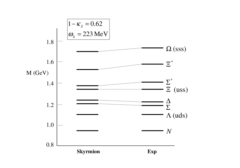
Figure 4: Strange hyperon spectrum in the skyrmion model compared with experiments (or equivalently nonrelativistic quark model): The parameter $\omega_{K}$ fixed by the state $\Lambda$ (marked by the star) and the $c_{K}$ by the empirical relation (II.188) are $\omega_{K}=223$ MeV and $c_{K}\equiv 1-\kappa_{s}=0.62$. This figure is an eyeball reproduction of the original figure in ELAF93.

2.2.4 Heavy-quark symmetry and skyrmions

Hyperfine splitting

One obvious feature in Figures II.2 and II.3 is that the hyperfine coefficients $c$ decrease as the heavy quark mass (or heavy-meson mass) increases. To be specific, let us consider the structure of baryons with one heavy quark $Q=s,s,b$ (we are considering the s quark to be heavy as mentioned above). From (II.187), we see that

$$\Sigma_{\mbox{\tiny Q}}-\Lambda_{\mbox{\tiny Q}}=\frac{1}{\cal I}(1-c_{\mbox{\tiny Q}})\simeq 195{\rm MeV}(1-c_{\mbox{\tiny Q}})$$ (II.190)

where the last equality is obtained from the $\Delta N$ mass splitting which fixes $1/{{\cal I}}$. This implies a simple relation for heavy-quark flavors $Q$ and $Q^{\prime}$

$$\frac{\Sigma_{Q}-\Lambda_{Q}}{\Sigma_{Q^{\prime}}-\Lambda_{Q^{\prime}}}\simeq\frac{1-c_{\mbox{\tiny Q}}}{1-c_{\mbox{\tiny Q}^{\prime}}}.$$ (II.191)

With the experimental value $\Sigma_{c}-\Lambda_{c}\approx 168{\rm MeV}$ for the charmed baryons, we get $c_{c}\simeq 0.14$ as given in Figure II.3. In the heavy-quark limit, we expect the hyperfine splitting to go to zero [71], so let us assume that

$$c_{\Phi}\approx am_{\Phi}^{-1}$$ (II.192)

where $\Phi$ stands for the heavy meson in which the heavy quark $Q$ is lodged and $a$ is a constant of mass dimension of $O(N_{c}^{0})$. Taking $m_{\mbox{\tiny D}}=1869{\rm MeV}$ in the charmed sector, we have $a\simeq 262$ MeV. So

$$c_{\mbox{\tiny Q}}\simeq 262{\rm MeV}/m_{\Phi}.$$ (II.193)

Now for b-quark baryons, using $m_{\mbox{\tiny B}}=5279$ MeV, we find $c_{b}\simeq 0.05$ which with (II.190) predicts

$$\Sigma_{b}-\Lambda_{b}\approx 185{\rm MeV}.$$ (II.194)

This agrees well with the quark-model prediction. Furthermore the $\Sigma^{*}-\Sigma$ splitting comes out correctly also. For instance, it is predicted that

$$\frac{\Sigma^{*}_{b}-\Sigma_{b}}{\Sigma^{*}_{c}-\Sigma_{c}}\simeq\frac{c_{b}}{c_{c}}\simeq\frac{m_{\mbox{\tiny D}}}{m_{\mbox{\tiny B}}}\approx 0.35$$ (II.195)

to be compared with the quark-model prediction $\sim 0.32$. If one assumes that the heavy mesons $\Phi$’s are weakly interacting, then we can put more than one heavy mesons in the soliton and obtain the spectra for $\Xi$’s and $\Omega$’s given in Figs. II.2 and II.3[72].

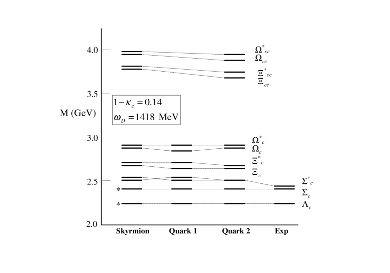
Figure 5: Charmed hyperon spectrum in the skyrmion model compared with quark-model predictions: Two parameters fixed by fitting two lowest experimental levels (marked by stars) are $\omega_{D}=1418$ MeV and $c_{D}\equiv 1-\kappa_{c}=0.14$. The parameters for the strange-quark sector are fixed from Figure II.2 “Quark model 1” is the prediction by L.A. Copley, N. Isgur and G. Karl, Phys. Rev. D20, 768 (1979) and K. Maltman and N. Isgur, Phys. Rev. D22, 1701 (1980) and “Quark model 2” is the prediction by A. De Rújula, H. Georgi and S.L. Glashow, Phys. Rev. D12, 147 (1975). This figure is an eyeball reproduction of the original figure in ELAF93.

2.2.5 Berry potentials in heavy-quark limit

The analysis made above suggests that the hyperfine splitting goes to zero in heavy quark limit as $O(N_{c}^{-1}m_{\Phi}^{-1})$. Here we will show that in the limit heavy-quark symmetry is restored, the Berry potential obtained in the last lecture vanishes, namely that $A=F=0$. To do this, we first construct the Lagrangian that possesses chiral symmetry and heavy quark symmetry, following Ref.[73].

Suppose that a meson is made up of a heavy quark $Q$ and a light antiquark $\bar{q}$. We denote the spin singlet $P$, the pseudoscalar used in the previous subsection and the spin triplet $P^{*}$. When the quark is light, then the $P^{*}$ is much heavier than $P$. For instance, the mass ratio $K^{*}/K\approx 0.5$. We understand this in terms of one-gluon exchange that pushes $P^{*}$ up above $P$ proportional to $(m_{q}m_{\mbox{\tiny Q}})^{-1}$. However as $m_{\mbox{\tiny Q}}\rightarrow\infty$, the $P$ and $P^{*}$ become degenerate. As a consequence, the heavy-quark spin that decouples from the spectrum becomes a good quantum number. This is the heavy-quark spin symmetry. Thus for a baryon containing a heavy quark $Q$, we need both $P$ and $P^{*}$ to construct a skyrmion in the Callan-Klebanov scheme if one wants to assure correct symmetry in heavy baryons. We will see that this degeneracy plays a key role in giving the correct Berry potential. An elegant way of incorporating the symmetry of $P$ and $P^{*}$ is to write the meson field as[74]

$$H=\frac{(1+\not\!{v})}{2}\left[{P^{*}}_{\mu}\gamma^{\mu}-P\gamma^{5}\right]$$ (II.196)

where $v_{\mu}$ is the four-velocity of the heavy quark. This field transforms as follows. Under chiral transformation $h$ (i.e, $\xi\rightarrow L\xi h^{\dagger}=h\xi R^{\dagger}$), it transforms

$$H\rightarrow Hh$$ (II.197)

which is equivalent to (II.150) generalized to the $H$ field and under heavy-quark spin symmetry $S$, it transforms as

$$H\rightarrow SH.$$ (II.198)

This is the symmetry we did not impose when we were discussing the Callan-Klebanov model. Writing in derivative expansion the Lagrangian density invariant simultaneously under the two symmetry transformations, we have

$${\cal L}^{\mbox{\tiny HQS}} = \frac{f^{2}}{4}{\mbox{Tr}}(\partial_{\mu}U\partial^{\mu}U^{\dagger})-i{\mbox{Tr}}\overline{H}_{a}v^{\mu}\partial_{\mu}H_{a}+i{\mbox{Tr}}\overline{H}_{a}H_{b}v^{\mu}\left(V_{\mu}\right)_{ba}$$ (II.199)

$$+ig{\mbox{Tr}}\overline{H}_{a}H_{b}\gamma^{\mu}\gamma_{5}\left(A_{\mu}\right)_{ba}+\cdots\ \ ,$$

where the subscript $a$ labels the light quark flavor and the “induced” vector and axial vector currents are given by

$$V_{\mu} = \frac{1}{2}(\partial_{\mu}\xi\xi^{\dagger}+\partial_{\mu}\xi^{\dagger}\xi),$$ (II.200)

$$A_{\mu} = \frac{1}{2i}(\partial_{\mu}\xi\xi^{\dagger}-\partial_{\mu}\xi^{\dagger}\xi)$$ (II.201)

with $\xi=\sqrt{U}$. The $g$ is an unknown axial vector coupling constant to be determined from experiments. The ellipsis stands for higher derivative terms and terms that break both chiral and heavy-quark symmetries. As written, the $H$ field has dimension 3/2 since a factor of $\sqrt{m_{\Phi}}$ has been incorporated into the component fields $P$ and $P^{*}$. The heavy meson mass term is cancelled away by the redefinition of the meson field $H\rightarrow e^{iv\cdot xm_{H}}H$ where $v_{\mu}$ is the velocity four vector.

We will now show that the vanishing of $c$ is tantamount to the disappearance of the associated nonabelian Berry potential that emerges from the Lagrangian (II.199). What happens is that the Berry phases generated from $P$ and $P^{*}$ when they are integrated out cancel exactly in the IW limit [75]. This is the analog of the vanishing Berry potential in the diatomic molecule when the electronic rotational symmetry is restored.

For the present purpose, it is convenient to rewrite (II.199) as

$${\cal L}_{H} = -i{\mbox{Tr}}\overline{H}_{a}v^{\mu}\partial_{\mu}H_{a}+i{\mbox{Tr}}\overline{H}_{a}H_{b}v^{\mu}\left(U^{\dagger}\partial_{\mu}U\right)_{ba}$$ (II.202)

$$+ig{\mbox{Tr}}\overline{H}_{a}H_{b}\gamma^{\mu}\gamma^{5}\left(U^{\dagger}\partial_{\mu}U\right)_{ba}+\frac{f^{2}}{4}{\mbox{Tr}}(\partial_{\mu}U\partial^{\mu}U^{\dagger})+\cdots$$

This is obtained from (II.199) by “dressing” $H$ with pion field as $H\rightarrow H\xi$. To $O(m_{Q}^{0}\cdot N_{c}^{0})$, we get the fine-structure spectrum by taking the hedgehog configuration $U_{c}$ in (II.202). In the infinite heavy-quark mass limit, the heavy meson is bound at the center of the soliton. Now we go to $O(m_{Q}^{0}\cdot N_{c}^{-1})$ by slowly rotating the hedgehog

$$U=S(t)U_{c}S^{\dagger}(t).$$ (II.203)

As we did in the case of the chiral bag, we let the rotation operator act on the $H$ field, thereby unwinding the soliton

$$H\rightarrow HS^{\dagger},\ \ \ \ \overline{H}\rightarrow S\overline{H}.$$ (II.204)

The Lagrangian (II.202) becomes

$${\cal L}_{H} = -i{\mbox{Tr}}\overline{H}\partial_{t}H-i{\mbox{Tr}}H\partial_{t}S^{\dagger}S\overline{H}+\frac{{\cal I}}{4}{\mbox{Tr}}(S^{\dagger}\partial_{t}S)^{2}$$ (II.205)

$$+i{\mbox{Tr}}\overline{H}_{a}H_{b}\left(S^{\dagger}(U^{\dagger}\partial_{t}U)S\right)_{ba}+ig{\mbox{Tr}}\overline{H}_{a}H_{b}\gamma^{o}\gamma^{5}\left(S^{\dagger}(U^{\dagger}\partial_{t}U)S\right)_{ba}$$

$$+ig{\mbox{Tr}}\overline{H}_{a}H_{b}\gamma^{i}\gamma^{5}\left(U_{c}^{\dagger}\partial_{i}U_{c}\right)_{ba}+\cdots\ \ .$$

Now one expects that the heavy meson is bound at the origin of the soliton; therefore the fourth and fifth terms of (II.205) vanish in the heavy-meson limit, so we are left with

$${\cal L}_{H} = -i{\mbox{Tr}}\overline{H}\partial_{t}H+\frac{{\cal I}}{4}{\mbox{Tr}}(S^{\dagger}\partial_{t}S)^{2}+-i{\mbox{Tr}}H\partial_{t}S^{\dagger}S\overline{H}$$ (II.206)

$$+ig{\mbox{Tr}}\overline{H}_{a}H_{b}\gamma^{i}\gamma^{5}\left(U_{c}^{\dagger}\partial_{i}U_{c}\right)_{ba}+\cdots\ \ .$$

In complete analogy with the diatomic molecule and the chiral bag, we can identify the second term of (II.206) with the Berry potential. As in the chiral bag case, $\dot{S}^{\dagger}S$ lives in the isospin space of the light-quark sector and hence operates on the space of the light antiquark $\bar{q}$. When the $H$ is bound to the soliton, the light antiquark is characterized by its grand spin $T=0$ where $\vec{T}=\vec{I}_{\bar{q}}+\vec{J}_{\bar{q}}$. This can be understood simply in the chiral bag model. In the chiral bag model, the lowest light-quark orbit is given by the hedgehog $T=0$. The heavy meson $Q\bar{q}$ is therefore made of a “hole” in the hedgehog and a (heavy) particle in the flavor $Q$ orbit. Thus the configuration of the light antiquark in $H$ takes the form

$$|T=0\rangle=\frac{1}{\sqrt{2}}\left(|\bar{d}\downarrow\rangle-|\bar{u}\uparrow\rangle\right).$$ (II.207)

Now the heavy particle decouples in the infinite mass limit, so behaves as a spectator and the role of fast variable is taken up entirely by the light antiquark, making it completely analogous to the quark sitting in $T=0$ orbit in the chiral bag model. We know from Lecture I that the operator $\dot{S}^{\dagger}S$ sandwiched between the $T=0$ states vanishes as one can readily verify with (II.207) acted on by an isospin operator. In other words, the Berry potential vanishes.

2.2.6 Comparison with large $N_{c}$ QCD

The general characteristics of the skyrmions, both the ground state (light-quark baryons) and the excited states (heavy-quarks baryons), can be understood in terms of large $N_{c}$ QCD. In large $N_{c}$ limit, the consistency in $N_{c}$ behavior as well as unitarity requires that the $O(1/N_{c})$ correction to the axial coupling constant $g_{A}$ or equivalently to the $\pi$-baryon coupling constant $g_{\pi NN}$ should vanish [76]. The leading nonvanishing correction comes at order $1/N_{c}^{2}$. This can happen only if there is an infinite tower of degenerate states contributing in the intermediate state in the limit of large $N_{c}$. The degeneracy is lifted at the order $1/N_{c}$. This can be seen by observing that the Born term for baryon-pion scattering violates both large $N_{c}$ constraint and unitarity, and hence must be cancelled – among the tower of intermediate states – to $O(1/N_{c})$ or alternatively by assuring that one loop chiral perturbation corrections to pion-baryon scattering do not violate the large $N_{c}$ constraint and unitarity.

A consequence of the Dashen-Manohar QCD constraints in light-quark baryons is found to be that baryon splittings must be proportional to $1/N_{c}$ and $\vec{J}^{2}$ where $J$ is the angular momentum of the baryon[77]. This is precisely the structure of the light-quark spectrum we obtained in the skyrmion picture. Now if the baryons contain one heavy quark $Q$ plus two light quarks, heavy-quark symmetry requires that the hyperfine splitting in the heavy baryons must be inversely proportional to the heavy-quark mass $m_{Q}$. Thus large $N_{c}$ QCD predicts the splitting to be $\sim(N_{c}m_{Q})^{-1}$. Furthermore from the Dashen-Manohar constraints, it follows [78] that the hyperfine splitting for, say, $\Sigma^{*}_{Q}-\Sigma_{Q}$ must be of the form, $\sim\vec{J}_{l}\cdot\vec{J}_{Q}$, where $J_{l}$ is the light-quark soliton angular momentum and $J_{Q}$ the heavy-quark angular momentum. This is identical to what we found in the heavy baryon spectrum (see (II.186))

$$\Delta H\sim\frac{1}{{\cal I}}c_{\Phi}\vec{J}_{l}\cdot\vec{J}_{\Phi}$$ (II.208)

where $J_{\Phi}$ is the angular momentum lodged in the Berry potential generated from the heavy meson $\Phi$ containing the heavy quark $Q$ when the latter is integrated out. (Recall that $c$ is of the form, Eq. (II.193).)

The same argument applies to non-relativistic quark models as one expects from the large $N_{c}$ equivalence between the skyrmion model and non-relativistic quark model[79].

Part III Chiral Symmetry in Nuclei

Updating Remark

[There has been an extensive activity in implementing chiral symmetry in nuclear physics since the time of the ELAF93 lectures. The recent developments are: (1) the skyrmion description of finite nuclei and nuclear matter; (2) effective field theory approach to few-nucleon systems (or dilute systems), nuclear matter and dense matter; (3) chiral restoration phase transition.

The Skyrme Lagrangian (II.11) has been investigated by mathematicians at classical level up to mass (or baryon) number $B\leq 22$ (e.g., see [141]) and the solutions were found to possess an intriguing geometrical structure. Although mathematically beautiful, it is not clear what the quantization will do to the solutions and whether the classical picture has anything to do with real nuclei. However the B=2 system is fairly well understood. In fact, the skyrmion description of the deuteron is a beautiful case of large $N_{c}$ QCD at work [142].

The modern development of an effective field theory for nuclei is described in subsection 3.7, that of the connection between a chiral Lagrangian field theory with BR scaling and Landau Fermi-liquid theory for nuclear matter in subsection 3.8 and that of hidden local symmetry theory in dense/hot matter in subsection 4.4.]

1 Introduction

In the preceding two lectures we discussed the structure of hadrons and their interactions in an isolated environment with a focus on chiral structure of the vacuum and light and heavy excitations on it. In this lecture, we turn to nuclei and nuclear matter and their interactions. We will focus on many-body systems with light-quark (up, down and strange ) hadrons only. We will not discuss the behavior of heavy baryons in medium. Broadly we can classify two classes of issues involved here. One is the change of the environment when there are many but finite number of baryons present in the system, thus addressing the issue of vacuum change in the medium and consequently modifications in the intrinsic property of the particles (both baryons and mesons) such as their masses and coupling constants. The other is the interaction of the particles among themselves, which is intrinsically many-body in nature. The question then is: Given an effective Lagrangian as discussed in Lectures I and II, with low-excitation mesons and baryons relevant at the energy scale below the chiral symmetry scale $\Lambda_{\chi}$, how do we describe nuclei and their interactions?

There are basically two ways of addressing this question. We will discuss both. The first described in the next section is to start with an effective Lagrangian given in large $N_{c}$ expansion as we have gotten in the previous lectures and develop many-body dynamics along the line that we have pursued for a baryon, that is to look at the multibaryon sector of the skyrmion picture. Unfortunately the mathematics of multibaryon structure is yet obscure and beyond baryon number 2, we have no clear understanding of the basic structure. There is a large number of literature on the infinite baryon number system, that is, nuclear matter, but again apart from a general global property, little is understood at the moment. In this chapter, we will treat the two-nucleon system, i.e, the deuteron and then nuclear force for which there is a promising new development that deserves to be recognized.

The second approach is to start with an effective Lagrangian that consists of mesons and baryons and guided by chiral symmetry and other symmetries of the strong interactions, develop chiral perturbation theory for nuclear dynamics. There is an inherent limitation to such an approach that is associated with low momentum/energy expansion. Nonetheless it has certain predictive powers as we shall show later. The main task then would be to understand nuclear forces from the point of view of chiral symmetry and then develop nuclear response functions in the same scheme. This approach will be discussed with applications to both finite nuclei and infinite nuclear matter, possible phase transitions under extreme conditions of density etc.

2 Nuclei As Skyrmions

Given a realistic effective Lagrangian of meson fields, the topological soliton sector should in principle give rise, not only to the baryons we considered above, but also to arbitrary winding-number objects. In the strong interactions, the winding number $W$ is the baryon number $n_{B}$ and hence we are to obtain nuclei with the baryon number $n_{B}=A$ where $A$ is the mass number of the nucleus when properly quantized. Unfortunately we have at present very little understanding of the structure of multi-skyrmion configurations. Given the approximations that one is forced to make in solving the problem, the question is how close the multi-winding-number solution is to real nuclei. We will discuss later an alternative approach of the skyrmion phenomenology that sidesteps solving this difficult problem. There the idea is to deduce an effective nucleon-nucleon potential using the skyrmion structure of the $n_{B}=2$ soliton and let the ensemble of $n_{B}=1$ solitons interact through the potential. This is closer to the conventional approach to the nucleus. In this Section, we discuss how much of nuclear properties we can understand solely from a skyrmion point of view. We discuss the simplest nucleus, the deuteron and then nucleon-nucleon potential. There are studies of $A\geq 3$ nuclei in terms of multi-winding-number skyrmions but the mathematics involved has not yet been worked out to the point as to be able to gauge whether such a description is realistic. We shall not pursue this approach any further . Also instead of working with a general, vector-meson-implemented Lagrangian, we will consider the simplest one, the original Skyrme Lagrangian discussed in Lecture II,

$${\cal L}_{skyrme}=\frac{f_{\pi}^{2}}{4}{\mbox{Tr}}\ [\partial_{\mu}U\partial^{\mu}U^{\dagger}]+\frac{1}{32g^{2}}{\mbox{Tr}}\ [U^{\dagger}\partial_{\mu}U,U^{\dagger}\partial_{\nu}U]^{2}+r{\mbox{Tr}}\ ({\cal M}U+h.c.)$$ (III.1)

with $f_{\pi}$ the pion decay constant and $g$ the Skyrme term constant related to vector meson gauge coupling discussed in Lecture II. The last term in (III.1) is the leading chiral symmetry-breaking term of $O(\partial^{2})$ in the “chiral counting” defined more precisely later. In dealing with nonstrange nuclear systems, $U$ will be the chiral field in $SU(2)$, so the Wess-Zumino term is missing from (III.1). Later we will consider the chiral field valued in $SU(3)$ in dealing with kaon-nuclear interactions. In what follows, one should keep in mind that in some sense, this is a Lagrangian that results from a large vector-meson mass limit of a Lagrangian with explicit vector mesons with the so-called Skyrme quartic term representing in some average sense the effect of all phenomenology. More sophisticated Lagrangians with vector mesons and baryon resonances bring about quantitative improvements but no qualitative changes. This was quite clear in hyperon phenomenology discussed in the preceding chapter.

2.1 Deuteron

Consider the simplest nucleus, the deuteron, which is a loosely bound proton-neutron system with a large quadrupole moment: a binding energy of 2.2 MeV and a root-mean-square radius of 2.095 fm. Since the two nucleons are on the average widely separated, we could start with the product ansatz for the chiral field with winding number 2. Let us put the centers of the two skyrmions symmetrically about the origin along the x axis. When the two nucleons are widely separated, a reasonable configuration for the system is the product form,

$$U_{1}(\vec{r}+s\hat{x})SU_{1}(\vec{r}-s\hat{x})S^{\dagger}$$ (III.2)

where $U_{1}$ is the hedgehog with baryon number 1 and $S$ is a constant (global) $SU(2)$ matrix describing the relative isospin orientation of the two skyrmions . The two skyrmions are separated along the $x$ axis by the distance of $2s$. It turns out from the early numerical studies[80] that the most attractive configuration is obtained when the isospin of one skyrmion is rotated by an angle of 180^∘ about an axis perpendicular to the $x$ axis (i.e, the axis of separation). Choosing the z axis for the rotation,

$$A=e^{i\pi\tau_{3}/2}=i\tau_{3}$$ (III.3)

the $n_{B}=2$ chiral field takes the form

$$U_{s}(x,y,z)=U_{1}(x+s,y,z)\tau_{3}U_{1}(x-s,y,z)\tau_{3}.$$ (III.4)

Let us see what symmetries this ansatz has [81]. With the explicit form for the single hedgehog $U_{1}=\exp(i\vec{\tau}\cdot\hat{r}F(r))$, it is easy to verify that it satisfies the following discrete symmetry relations

$$U_{s}(-x,y,z) = \tau_{2}U_{s}^{\dagger}(x,y,z)\tau_{2},$$ (III.5)

$$U_{s}(x,-y,z) = \tau_{1}U_{-s}^{\dagger}(x,y,z)\tau_{1},$$ (III.6)

$$U_{s}(x,y,-z) = U_{-s}^{\dagger}(x,y,z).$$ (III.7)

It also has the symmetry under the parity transformation

$$U_{s}^{\dagger}(-x,-y,-z)=\tau_{3}U_{s}(x,y,z)\tau_{3}.$$ (III.8)

These discrete symmetries can be summarized by one nontrivial one

$$U_{s}(x,-y,-z)=\tau_{1}U_{s}(x,y,z)\tau_{1}.$$ (III.9)

What this says is that a spatial rotation about the axis of separation by angle of $\pi$ is equivalent to an isospin rotation about the $x$ axis by $\pi$. This symmetry forbids the quantum number $I=J=0$ where $I$ is the isospin and $J$ the angular momentum of the state. This is consistent with Pauli exclusion principle. However the product ansatz is not a solution of the equation of motion and in addition there is nothing to prevent another deuteron-like state (say, $d^{\prime}$) with $I=0$ and $J=1$ to appear nearly degenerate with the deuteron. Indeed a simple analysis does show that a $d^{\prime}$ is present when the product ansatz is used. In Nature there is only one bound state, so while the product ansatz describes the deuteron property (and more generally static two-nucleon properties [82]) in qualitative agreement with experiments, it does not have enough symmetry of Nature. In addition to the symmetry (III.9)

$$U_{2}(x,-y,-z)=\tau_{1}U_{2}(x,y,z)\tau_{1},$$ (III.10)

other discrete symmetries not present in the product ansatz but needed to eliminate the spurious $d^{\prime}$ are

$$U_{2}(-x,y,-z) = \tau_{1}U_{2}(x,y,z)\tau_{1},$$ (III.11)

$$U_{2}(-x,-y,z) = U_{2}(x,y,z).$$ (III.12)

(We are using the subscript 2 to indicate the winding number-2 configuration.) In fact the last symmetry (III.12) is a special case (i.e, $\alpha=\pi$) of the continuous cylindrical symmetry

$$U_{2}(\rho,\phi+\alpha,z)=e^{-i\alpha\tau_{3}}U_{2}(\rho,\phi,z)e^{i\alpha\tau_{3}}$$ (III.13)

where the $z$ axis is taken to be the symmetry axis. This has a toroidal geometry. A $n_{B}=2$ skyrmion with the symmetries (III.10), (III.11), (III.12) and (III.13) is found to be the lowest energy solution of the skyrmion equation[83]. With this configuration, there is no bound $d^{\prime}$ state as it is pushed up by rotation. We will refer to this as toroidal skyrmion. To be more quantitative, let us see what the classical energies of various configurations come out to be[50]. For this we put the length in units of $(ef)^{-1}$ and the energy in units of $f/2e$. In these units, the energy of two infinitely separated skyrmions is $1.23\times 24\pi^{2}$ whereas the toroidal structure with coincident skyrmions comes slightly lower, at $1.18\times 24\pi^{2}$. The latter corresponds to the lowest energy solution of the $n_{B}=2$ skyrmion. The $n_{B}=2$ spherical hedgehog configuration has much higher energy, $1.83\times 24\pi^{2}$.

The question is: What is the deuteron seen in Nature? While lowest in energy, the toroidal configuration cannot be the dominant component of the deuteron. For with that configuration, the size – and hence the quadrupole moment – of the deuteron would be much too small[87], the calculated size being $\sqrt{\langle r^{2}\rangle_{d}}\approx 0.92$ fm while experimentally it is $2.095$ fm and the calculated quadrupole moment being $Q\approx 0.082$ fm² while experimentally it is $0.2859$ fm². This compactness of the structure is easily understandable in terms of much too large binding energy – about an order of magnitude too large – associated with this configuration. Clearly then this configuration must constitute only a small component of the deuteron wave function. Despite the problem alluded above, the size and quadrupole moment indicate that the widely separated configuration should be closer to Nature. Even so, the deuteron seems to share the torus symmetry in a variety of ways as observed in its static electromagnetic properties and other moments.

Even though reducing the problem from a field theory involving solitons to a quantum mechanics in “moduli space” brings in enormous simplification, the reality must still be rather complex in terms of skyrmion configurations. A realistic treatment[50, 85] must encompass the unstable spherical hedgehog with winding number 2 [51], the manifold of which is twelve dimensional including six unstable modes, the infinitely separated two skyrmion configuration – which is also twelve dimensional – and the eight-dimensional toroidal configuration [83]. This is a very difficult problem and it is very unlikely that we will see analytical solutions in the near future. It is however expected that numerical simulations will provide accurate solutions within a near future. Indeed an initial “experiment” of that type has been recently performed. While the result is only preliminary and semiquantitative at best, it is nonetheless a remarkable development. Since it is most likely to be soon superseded by more refined results, we will not go into the details of the present calculation. Let it suffice to summarize what has been achieved so far[86]. In this analysis, initially two widely separated skyrmions (which are not a solution on a finite lattice which they are using) are prepared by relaxation. The continuum solution is imposed on the lattice. As the skyrmions relax, they approach each other through the dissipation of their orbital energy. At the point of closest approach, the two skyrmions merge into the optimal toroidal configuration and then scatter at angle $\pi/2$, a feature generic of two solitons scattering at low energy, such as monopole-monopole, skyrmion-skyrmion and vortex-vortex scattering. This process is found to repeat, with the skyrmions falling into the toroidal form and scattering at right angles. At each cycle, energy is transferred from the orbital motion to a radial excitation of the individual skyrmion. Quantizing the nearly periodic motion, it is found that for large $g^{2}$ (for which the Skyrme quartic term emerges from the $\rho$ meson kinetic energy term in a more realistic hidden gauge symmetry Lagrangian[48]), there is only one bound state with $J=1$ and $I=0$, with an unbound $J=0$ and $I=1$ state nearby. (There are instead many bound states for weak $g^{2}$. But for a weak $g^{2}$, there is no reason why the Skyrme Lagrangian would be a good approximation.) The bound wavefunction describes a state peaked at a configuration with two nucleons widely separated, hence elongated, with the size about twice that of the static toroidal structure and a quadrupole moment about 4 times. These are all in semiquantitative agreement with experiments.

2.2 Nuclear Forces

The static minimum-energy configuration is known to be tetrahedron for $n_{B}=3$, octahedron for $n_{B}=4$ etc.[87]. It would undoubtedly be most exciting to see what happens when one extends the sort of analysis made on the torus configuration of the deuteron to ³He, ⁴He etc. Unfortunately this will take a tour-de-force computational effort and extending beyond would probably be impossible except for qualitative features. As in the case of the torus, these configurations will make up only a small component of the wavefunctions even though symmetries may be correctly described by them. The alternative to this – which is definitely more economical and more predictive– is to construct a nucleon-nucleon potential from skyrmion structure and treat the nuclei in the conventional way. Furthermore, constrained static solutions that are required for constructing NN potentials are much easier to work out than the time-dependent problem mentioned above. The question that is properly posed is: Can one derive a nucleon-nucleon potential which is close to, say, the Paris potential[88] ?

The $n_{B}=2$ baryon has twelve collective degrees of freedom: three for translation (or center-of-mass position), three for orientations in space and isospin space, three for the spatial separation and three for the relative orientation in isospin. For the asymptotic configuration where two skyrmions are widely separated, the twelve degrees of freedom correspond to the coordinate $\vec{r}_{i}$ and the isospin orientation $S_{i}$ for each skyrmion $i=1,2$. When quantized, they represent two free nucleon states. The product ansatz possessing twelve collective degrees of freedom is close to two free nucleons when widely separated but lacks the correct symmetry at short distance. When two skyrmions are on top of each other, as mentioned above, the lowest energy configuration is that of a torus (with axial symmetry) with eight collective degrees of freedom. Thus four additional collective degrees of freedom are needed for describing general $n_{B}=2$ configurations. This constitutes the moduli space that is involved for the problem.

For general $n_{B}=2$ configurations, global collective coordinates do not affect the energy, so for considering a potential, we may confine ourselves to the separation $r$ of the two skyrmions and the relative isospace orientation which can be expressed by three Euler angles $\alpha$, $\beta$ and $\gamma$

$$C=S_{1}^{\dagger}S_{2}=e^{i\tau_{3}\alpha/2}e^{i\tau_{2}\beta/2}e^{i\tau_{3}\gamma/2}.$$ (III.14)

When global collective coordinates are quantized, the resulting Hamiltonian involves a potential which will then depend only on the separation $r$ which we choose here to be along the $z$ axis and the three Euler angles. The potential therefore must be expressible in terms of the Wigner ${\cal D}$-functions as[89]

$$V(r,C)=\sum_{j=0}^{\infty}\sum_{m=-j}^{j}\sum_{n=-j}^{j}V_{jmn}(r){\cal D}^{(j)}_{m,n}(C).$$ (III.15)

This is the most general form since the ${\cal D}$ functions form a complete set over $SU(2)$ for integer $j$. This can be further reduced by using the symmetry associated with rotation about the $z$ axis – therefore reducing the Euler angles to two, namely, $\beta$ and $(\alpha-\gamma)$ –and the relation $V(r,C)=V(r,C^{\dagger})$ due to the $SU(2)$ symmetry, to the form

$$V(r,C)=\sum_{j=0}^{\infty}\sum_{m=0}^{j}V_{jm}\frac{1}{2}\left[{\cal D}^{(j)}_{m,m}(C)+{\cal D}^{(j)}_{-m,-m}(C)\right].$$ (III.16)

The nucleon-nucleon potential can then be defined by taking the matrix element with the asymptotic two-nucleon wavefunction

$$\Psi(1,2)\sim{\cal D}^{(1/2)}_{i_{1},-s_{1}}(S_{1}){\cal D}^{(1/2)}_{i_{2},-s_{2}}(S_{2}).$$ (III.17)

The potential so defined is guaranteed to give the correct asymptotic behavior shared by the product ansatz and the correct short-distance behavior shared by the toroidal configuration. Although there is no rigorous proof, it appears that only the partial waves $j\leq 1$ contribute significantly[89]. Thus ignoring the higher partial waves $j\geq 2$, we have

$$V(r,C)=V_{00}(r){\cal D}^{(0)}_{0,0}(C)+V_{10}{\cal D}^{(1)}_{0,0}(C)+V_{11}(r)[{\cal D}^{(1)}_{1,1}(C)+{\cal D}^{(1)}_{-1,-1}(C)]$$ (III.18)

which when sandwiched with the wavefunction (III.17) gives

$$V(1,2)=V_{C}(r)+V_{SS}(r)\vec{\tau}_{1}\cdot\vec{\tau}_{2}\vec{\sigma}_{1}\cdot\vec{\sigma}_{2}+V_{T}(r)\vec{\tau}_{1}\cdot\vec{\tau}_{2}(3\vec{\sigma}_{1}\cdot\hat{r}\vec{\sigma}_{2}\cdot\hat{r}-\vec{\sigma}_{1}\cdot\vec{\sigma}_{2})$$ (III.19)

with

$$V_{C}=V_{00},\ \ \ V_{SS}=25(V_{10}+V_{11})/247,\ \ \ V_{T}=25(2V_{10}-V_{11})/486$$ (III.20)

with potential functions $V_{i}$ given by the skyrmion solution of the classical equation of motion. The $V$’s are obtained numerically.

There is considerable uncertainty in defining the separation $r$ between two skyrmions because of their extended structure. A convenient definition is [89]

$$(\frac{r}{2})^{2}=\frac{1}{n_{B}}\int d^{3}x\vec{x}^{2}{\cal B}^{0}(\vec{x})$$ (III.21)

where ${\cal B}^{0}$ is the baryon number density. This reduces to the usual separation $r=|\vec{r}_{1}-\vec{r}_{2}|$ if one takes the form

$${\cal B}^{0}(\vec{x})=\delta^{3}(\vec{x}+\frac{1}{2}r\hat{e}_{3})+\delta^{3}(\vec{x}-\frac{1}{2}r\hat{e}_{3}).$$

The resulting central $V_{c}^{T}$ potentials obtained by Walhout and Wambach [89] and Walet and Amado [90] qualitatively agree with with realistic phenomenological potentials. The intermediate-range attraction in the central potential obtained in these calculations has been the most difficult one to obtain in the skyrmion picture. (Other components of the force have been better understood.) This difficulty is now largely eliminated. A considerable improvement is obtained by introducing state-mixing between NN, N$\Delta$ and $\Delta\Delta$ intermediate states that involves $1/N_{c}$ corrections[90].

In summary, the skyrmion picture is found[91] to provide a generally satisfactory account of long-range pion exchange, short-distance repulsion, tensor forces and spin-orbit forces. Considering the enormous simplicity of the effective Lagrangian, this is a truly remarkable success of the model.

3 Chiral Perturbation Theory

3.1 Foreword

Chiral symmetry has played indirectly an extremely important and powerful role in nuclear physics since many years [92]; yet it is only recently that the nuclear physics community started to pay attention to this, particularly in connection with the structure of the nucleon and associated issues. Even the role of mesons in nuclei – a problem which has been around for more than four decades – has only recently been elucidated, thanks largely to a better understanding of the workings of chiral symmetry in strongly interacting many-body systems. Though chiral symmetry addresses specifically to pions, it turns out to play a crucial role where other degrees of freedom than pions intervene. The reason for this is that pions dominate whenever they can and if they do not, then there are reasons for it, which have something to do with chiral symmetry.

In this part of the lecture, we discuss to what extent nuclear dynamics – both under normal and extreme conditions – are dictated by chiral symmetry. There are several layers of problems dealing with nuclei. The first is the property of the basic building block of the nucleus, which is of course the nucleon and the nucleon is made of quarks and gluons: We have to understand what the nucleon is to understand how two or more nucleons interact. Now given our understanding of the nucleon, we have to understand how they interact – following what symmetries and dynamics – and how the individual property of the nucleon is modified by the change of environment. In all these, we would like that the same guiding principles apply for both the basic structure of the nucleon and the residual interaction between them.

We shall discuss from the vantage point of chiral symmetry what the state of hadronic matter may be at densities near that of nuclear matter $\rho_{0}\approx 0.16fm^{-3}$ and ultimately higher including the regime $\rho\gg\rho_{0}$ where phase transitions from normal hadronic matter to “abnormal” matters are supposed to take place.

3.2 Chiral Lagrangians for Baryons and Goldstone Bosons

In Lecture II, we dealt with chiral Lagrangians with mesons only. We discussed there how baryons could emerge from meson fields as solitons (skyrmions). We saw that this picture of the baryons gets sharpened for large $N_{c}$. In principle, given such mesonic Lagrangians, we could expect to calculate properties of an A-skyrmion system and suitably quantized, to describe a nucleus with A nucleons. A brief discussion on this matter was given in the preceding section. One day it may be possible to describe, say, ²⁰⁸Pb with a Lagrangian whose parameters are completely fixed in the zero-baryon sector. In fact we might be able to expect that the Pb nucleus is understood because the nucleon is understood, through a concept of “tumbling” as stressed by Nambu[1], the idea being that it is a hierarchy of symmetries which tumble down from high energy to low energy with the strength of the condensates setting the scale. The key picture of such a hierarchy is a $\sigma$-model structure, which applies to the Higgs sector, to the QCD sector (nucleon), to the complex nuclear sector and to superconductivity. In Lecture I, we discussed the possibility that a hierarchy of induced gauge potentials might provide the link.

In this lecture, we approach the problem from a different vantage point. We shall assume that it is possible to map the soliton-meson Lagrangian that results from the soliton quantization and fluctuations around it to an effective Lagrangian of baryons and mesons. In large $N_{c}$ limit, the baryons are infinitely massive, so one can do a simultaneous expansion in $1/m_{\mbox{\tiny B}}$ (where $m_{\mbox{\tiny B}}$ is the baryon mass), $\partial/\Lambda_{\chi}$ and ${\cal M}/\Lambda_{\chi}$ (where ${\cal M}$ is the quark mass matrix). The baryon here is put in a way quite analogous to the heavy quark in the chiral symmetric heavy quark Lagrangian considered in the preceding lecture.

We will construct an appropriate Lagrangian in the spirit of chiral expansions. In so doing, we will postulate that mesons and baryons that figure in nuclei satisfy chiral symmetry and other flavor symmetries. We will simply write it with local fields. The underlying assumption is that Weinberg’s “theorem” [93] holds equally in the case that baryons are present explicitly. In this framework, the effective Lagrangian approach is as general as any field theory.

Although for the moment we will be mostly concerned with the up- and down-quark ($SU_{f}(2)$) sector, we shall write the Lagrangian for the $SU(3)$ flavor as it will be needed for kaon-nuclear interactions and kaon condensation in the later part of the lecture. As explained in the previous lectures, the $U_{A}(1)$ symmetry is broken by anomaly, so the associated ninth pseudoscalar meson $\eta^{\prime}$ is massive. It will not concern us here. The scale invariance is broken by the trace anomaly with the associated scalar $\chi$ playing an important role for scale properties of the hadrons. This feature will be incorporated later in the scheme. Let the octet pseudoscalar field $\pi=\pi^{a}T^{a}$ be denoted by

$$\sqrt{2}\pi=\left(\begin{array}[]{ccc}\frac{1}{\sqrt{2}}\pi^{0}+\frac{1}{\sqrt{6}}\eta&\pi^{+}&K^{+}\\ \pi^{-}&-\frac{1}{\sqrt{2}}\pi^{0}+\frac{1}{\sqrt{6}}\eta&K^{0}\\ K^{-}&\bar{K}^{0}&-\frac{2}{\sqrt{6}}\eta\end{array}\right)$$ (III.4)

and the octet baryon field $B=B^{a}T^{a}$ be given by

$$B=\left(\begin{array}[]{ccc}\frac{1}{\sqrt{2}}\Sigma^{0}+\frac{1}{\sqrt{6}}\Lambda&\Sigma^{+}&p\\ \Sigma^{-}&-\frac{1}{\sqrt{2}}\Sigma^{0}+\frac{1}{\sqrt{6}}&n\\ \Xi^{-}&\Xi^{0}&-\frac{2}{\sqrt{6}}\Lambda\end{array}\right).$$ (III.8)

Define as before the “induced” vector current $V_{\mu}$ and axial-vector vector current $A_{\mu}$

$$\left(\begin{array}[]{c}V^{\mu}\\ -iA^{\mu}\end{array}\right)=\frac{1}{2}\left(\xi^{\dagger}\partial^{\mu}\xi\pm\xi\partial^{\mu}\xi^{\dagger}\right)$$ (III.11)

where $U=\xi^{2}={\rm exp}(2i\pi^{a}T^{a}/f)$ with ${\mbox{Tr}}T^{a}T^{b}=\frac{1}{2}\delta_{ab}$ (i.e, $T^{a}\equiv\lambda^{a}/2$ where $\lambda^{a}$ are the usual Gell-Mann matrices). Recall: Since $U$ transforms $U\rightarrow LUR^{\dagger}$ under chiral transformation with $L\in SU_{L}(3)$ and $R\in SU_{R}(3)$, $\xi$ transforms $\xi\rightarrow L\xi g^{\dagger}(x)=g(x)\xi R^{\dagger}$ with $g\in SU(3)$ a local, nonlinear function of $L$, $R$ and $\pi$. Under the local transformation $g(x)$, $V_{\mu}$ transforms as a gauge field

$$V_{\mu}\rightarrow g(V_{\mu}+\partial_{\mu})g^{\dagger}$$ (III.12)

while $A_{\mu}$ transforms homogeneously (or covariantly)

$$A_{\mu}\rightarrow gA_{\mu}g^{\dagger}.$$ (III.13)

The next thing to do is to decide how the baryon field transforms under chiral $SU_{L}(3)\times SU_{R}(3)$ symmetry. Now the baryon field can be considered as a matter field just as the vector meson fields $\rho$ are. The general theory of matter fields interacting with Goldstone boson fields was formulated by Callan, Coleman, Wess and Zumino many years ago [94]. Since matter fields transform as definite representations only under the unbroken diagonal subgroup $SU_{L+R}(3)$, one may choose any representation that reduces to this subgroup. Different choices give rise to the same S-matrix. A convenient choice turns out to have the baryon field transform

$$B\rightarrow gBg^{\dagger}.$$ (III.14)

Under vector transformation $L=R=V$, we have $g=V$ so that Eq.(III.14) reduces to the desired vector (octet) transformation $B\rightarrow VBV^{\dagger}$. With this representation, the pion field has only derivative coupling to the baryons which facilitates the chiral counting developed below. [95]. With the “gauge” field $V_{\mu}$, we write the covariant derivative

$$D^{\mu}B=\partial^{\mu}+[V^{\mu},B]$$ (III.15)

which transforms $D^{\mu}B\rightarrow gD^{\mu}Bg^{\dagger}$. The Lagrangian containing the lowest derivative involving baryon fields is then

$${\cal L}_{B} = i{\mbox{Tr}}(\bar{B}\gamma^{\mu}D_{\mu}B)-m_{B}{\mbox{Tr}}(\bar{B}B)$$ (III.16)

$$+ D{\mbox{Tr}}(\bar{B}\gamma_{\mu}\gamma_{5}\{A^{\mu},B\})+F{\mbox{Tr}}(\bar{B}\gamma_{\mu}\gamma_{5}[A^{\mu},B])+O(\partial^{2})$$

where $D$ and $F$ are constants to be determined from experiments as we will see later. The mesonic sector is of course described by Eq. (III.1), the chirally invariant part of which is, in terms of the chiral field $U$ alone,

$${\cal L}^{U}=\frac{f_{\pi}^{2}}{4}{\mbox{Tr}}(\partial_{\mu}U\partial^{\mu}U^{\dagger})+O(\partial^{4}).$$ (III.17)

In Eqs.(III.16) and (III.17), truncation is made at the indicated order of derivatives.

Next we need to introduce chiral symmetry breaking terms since the symmetry is indeed broken by the quark mass terms. We assume as suggested by QCD Lagrangian that the quark mass matrix ${\cal M}$ transforms as $(3,\bar{3})+(\bar{3},3)$, namely, as

$${\cal M}\rightarrow L{\cal M}R^{\dagger}.$$ (III.18)

In our discussion, the mass matrix will be taken to be in the diagonal form

$${\cal M}={\rm diag}\ (m_{u},m_{d},m_{s}).$$ (III.19)

Writing terms involving ${\cal M}$ that transform invariantly under chiral transformation, we have

$${\cal L}_{\chi SB} = r{\mbox{Tr}}\ ({\cal M}U+h.c.)$$

$$+ a_{1}{\mbox{Tr}}\overline{B}\left(\xi{\cal M}\xi+h.c.\right)B+a_{2}{\mbox{Tr}}\overline{B}B\left(\xi{\cal M}\xi+h.c.\right)+a_{3}{\mbox{Tr}}\overline{B}B{\mbox{Tr}}\left({\cal M}U+h.c.\right).$$

In writing this only $CP$ even terms are kept. In general, without restriction on $CP$, the $h.c.$ term would be multiplied by complex conjugation of the coefficient which would in general be complex. As detailed later, the mass matrix ${\cal M}$ is formally $O(\partial^{2})$, so to the order involved in (LABEL:sbp), we have to implement with a Lagrangian that contains two derivatives. We will call it $\delta{{\cal L}_{B}}$. It will be specified below.

As given, the baryon Lagrangian (III.16) does not lend itself to a straightforward chiral expansion. This is because the baryon mass $m_{B}$ is not small compared with the chiral scale $\Lambda_{\chi}$: As noted below, while the space derivative acting on the baryon field can be considered to be small, the time derivative cannot be considered to be so since it picks up the baryon mass term. It is therefore more appropriate to consider the baryon to be “heavy” and make a field redefinition so as to eliminate the mass term from the Lagrangian. To do this we let [96]

$$B\rightarrow e^{im_{B}v\cdot x}\frac{1+\gamma\cdot v}{2}B$$ (III.21)

where $v_{\mu}$ is the velocity four-vector of the baryon with $v^{2}=1$. This rescaling eliminates the centroid mass dependence $m_{B}$ from the baryon Lagrangian ${{\cal L}}_{B}$ and banish negative-energy Dirac components $\frac{1}{2}(1+\gamma\cdot v)B$ to $1/m_{B}$ corrections

$${\cal L}_{B}={\mbox{Tr}}\overline{B}iv\cdot DB+2D{\mbox{Tr}}\overline{B}S^{\mu}\{A_{\mu},B\}+2F{\mbox{Tr}}\overline{B}[A_{\mu},B]+\cdots$$ (III.22)

and simplifies $\delta{{\cal L}_{B}}$ which is somewhat awesome looking to

$$\delta{\cal L}_{B} = c_{1}{\mbox{Tr}}\overline{B}D^{2}B+c_{2}{\mbox{Tr}}\overline{B}(v\cdot D)^{2}B+d_{1}{\mbox{Tr}}\overline{B}A^{2}B+d_{2}{\mbox{Tr}}\overline{B}(v\cdot A)^{2}B+\cdots$$

$$+ f_{1}{\mbox{Tr}}\overline{B}(v\cdot D)(S\cdot A)B+f_{2}{\mbox{Tr}}\overline{B}(S\cdot D)(v\cdot A)B+f_{3}{\mbox{Tr}}\overline{B}[S^{\alpha},S^{\beta}]A_{\alpha}A_{\beta}B+\cdots$$

where the ellipsis stands for other terms of the same class as well as $1/m_{B}$ corrections which are of the same order as the symmetry-breaking term (LABEL:sbp), that is, $O(\partial^{2})$. Here $S_{\mu}$ is the spin operator defined as $S_{\mu}=\frac{1}{4}\gamma_{5}[\not\!\!{v},\gamma_{\mu}]$ constrained to $v\cdot S=0$ and the constants $a_{i}$, $c_{i}$, $d_{i}$, $f_{i}$ and $r$ are parameters to be fixed from experiments.

In many-body systems like nuclei, we have to include also terms higher order in baryon field, such as[97]

$${\cal L}_{4}=\sum_{i}{\mbox{Tr}}\left(\overline{B}\Gamma_{i}B\right)^{2}+\cdots$$ (III.24)

where $\Gamma_{i}$ are matrices constrained by flavor and Lorentz symmetries which we assume do not contain derivatives. The ellipsis stands for four-fermion interactions containing derivatives and also for higher-fermion interaction terms. Such terms with quartic fermion fields can be thought of as arising when meson exchanges with the meson mass greater than the chiral scale are eliminated. We have already encountered such a term in Lecture II in connection with the $\eta^{\prime}$ exchange between baryons. We can also have derivatives multiplying $\Gamma_{i}$. We will encounter such derivative-dependent four-fermion terms later on – as counter terms – when we consider nuclear responses to electroweak interactions at which time we shall write down the explicit forms.

In the form given above for ${\cal L}_{B}$ and $\delta{\cal L}_{B}$, derivatives on the baryon field pick up small residual four-momentum $k_{\mu}$

$$p^{\mu}=m_{B}v^{\mu}+k^{\mu}.$$ (III.25)

In this form, a derivative on the baryon field is of the same order as a derivative on a pseudoscalar meson field or the mass matrix $\sqrt{{\cal M}}$.

The Lagrangian we will work with then is the sum of (III.17), (III.22), (LABEL:deltalb) and (III.24)

$${\cal L}={\cal L}^{U}+{\cal L}_{B}+\delta{\cal L}_{B}+{\cal L}_{4}.$$ (III.26)

Now given this Lagrangian for three-flavor system, it is easy to reduce it to one for two flavors – which is what we need for most of nuclear physics applications. The pseudoscalar field is then a $2\times 2$ matrix

$$\sqrt{2}\pi=\left(\begin{array}[]{cc}\frac{1}{\sqrt{2}}\pi^{0}&\pi^{+}\\ \pi^{-}&-\frac{1}{\sqrt{2}}\pi^{0}\end{array}\right)$$ (III.29)

and the baryon field becomes a simple doublet

$$N=\left(\begin{array}[]{c}p\\ n\end{array}\right)$$ (III.32)

with the resulting Lagrangian

$${\cal L} = N^{\dagger}i\partial_{0}N+iN^{\dagger}V_{0}N-g_{A}N^{\dagger}\vec{\sigma}\cdot\vec{A}N$$ (III.33)

$$+ bN^{\dagger}\left(\xi{\cal M}\xi+h.c.\right)N+h^{\prime}N^{\dagger}N{\mbox{Tr}}\left({\cal M}U+h.c.\right)+\cdots.$$

$$+ \sum_{i}(N^{\dagger}\Gamma_{i}N)^{2}+\delta{\cal L}_{B}\cdots$$

where we have replaced $(F+D)$ by $g_{A}$, relevant for neutron beta decay, a procedure which is justified at the tree order. This relation no longer holds, however, when loop corrections are included. This Lagrangian (III.33) will be used in nuclear physics applications in what follows.

So far, we have written down Lagrangian terms that are lowest in derivatives and in the quark mass matrix ${\cal M}$. Going further in the expansion can be done in two ways: one, higher derivatives in pseudoscalar fields (and higher orders in ${\cal M}$); two, introduce vector fields (and higher orders in ${\cal M}$). For instance, we can take the vector and axial-vector fields to be $O(\partial)$ and if they are coupled to the lowest derivatives on pseudoscalars consistent with chiral transformation, then we wind up with a Lagrangian valid up to $O(\partial^{4})$, e.g., the vector meson field tensor which involves $(\partial_{\mu}V_{\nu})^{2}$. In all applications we will discuss, we will follow the second route which is simpler at low orders we use.

3.3 Chiral Power Counting

In nuclear physics, we are concerned with an amplitude that involves $E_{N}$ nucleon lines (sum of incoming and outgoing lines), $E_{\pi}$ pion lines and one electroweak current. Chiral Lagrangian approach is relevant at low energy and low momentum, so we are primarily concerned with slowly varying electroweak fields. In dealing with chiral power counting, the pion field and its coupling are simple because chiral symmetry requires derivative coupling. The chiral field $U$ can be counted as $O(1)$ in chiral counting, a derivative acting on the pion field as $O(Q)$ where $Q$ is a characteristic pion four-momentum involved in the process, assumed to be of $O(m_{\pi})$ or less – and in any case much less than the chiral scale of order 1 GeV – and $m_{q}\sim m_{\pi}^{2}\sim O(Q^{2})$. As remarked above, the situation with the baryon as given in (III.16) is somewhat more complicated because the baryon mass is of $O(1)$ relative to the chiral scale. Indeed, one should count $m_{B}\sim O(1)$, the generic baryon field $\psi\sim O(1)$ and hence $\partial^{\mu}\psi\sim O(1)$. This means that

$$(i\gamma_{\mu}\partial^{\mu}-m_{B})\psi=iv_{\mu}\partial^{\mu}N\sim O(Q).$$ (III.34)

However the three-momentum of the baryon – and hence the space derivative of the baryon field – should be taken to be $O(Q)$ while the time derivative of it should be taken to be $O(1)$. The heavy-fermion formalism takes care of this problem of the heavy baryon mass. We will illustrate how this works out in specific examples we will treat later.

In deducing the chiral counting rule, we must distinguish two types of graphs: one, reducible graphs and the other, irreducible graphs. Chiral expansion is useful for the second class of diagrams. An irreducible graph is a graph that cannot be made into disconnected graphs by cutting any intermediate state containing $E_{N}/2$ nucleon lines and either all the initial pions or all the final pions. Reducible graphs involve energy denominators involving the difference in nucleon kinetic energy which is much smaller than the pion mass whereas irreducible graphs involve energy denominators of $O(Q)$ or the pion mass. We must apply chiral perturbation theory to the irreducible graphs, but not to the reducible ones. The reducible ones involve infrared divergences and are responsible for such nonperturbative effect as binding or pairing transitions. In the language of effective field theories [2] it is the effect of reducible graphs that transform “irrelevant terms” to “marginal” leading to interesting phenomena such as superconductivity as discussed in Polchinski’s lecture and elsewhere. In the present context, the reducible graphs are included when one solves Lippman-Schwinger equation or Schrödinger equation. We will therefore confine ourselves to the irreducible graphs only.

Furthermore the counting rule is much more clearly defined without vector mesons than with vector mesons. The vector mesons with their mass comparable to the chiral scale bring in additional scale to the problem.

In what follows, using heavy-fermion formalism (HFF), we rederive and generalize somewhat Weinberg’s counting rule applicable to irreducible graphs [93, 97, 98]. Although we shall not consider explicitly the vector-meson degrees of freedom, we include them here in addition to pions and nucleons. Much of what we obtain later turn out to be valid in the presence of vector mesons. Now in dealing with them, their masses will be regarded as comparable to the characteristic mass scale of QCD $\sim 4\pi f_{\pi}$ which can be considered heavy compared to $Q$ – say, scale of external three momenta or $m_{\pi}$ .
In establishing the counting rule, we make the following key assumptions: Every intermediate meson (whether heavy or light) carries a four-momentum of order of $Q$ while every intermediate nucleon carries a four-momentum of order of $m_{N}$, namely, of the QCD scale. In addition we assume that for any loop, the effective cut-off in the loop integration is of order of $Q$. We will be more precise as to what this means physically when we discuss specific processes, for this clarifies the limitation of the chiral expansion scheme.

An arbitrary Feynman graph can be characterized by the number $E_{N}(E_{H})$ of external – both incoming and outgoing – nucleon (vector-meson) lines, the number $L$ of loops, the number $I_{N}(I_{\pi},\ I_{H})$ of internal nucleon (pion, vector-meson) lines. Each vertex can in turn be characterized by the number $d_{i}$ of derivatives and/or of $m_{\pi}$ factors and the number $n_{i}$ $(h_{i})$ of nucleon (vector-meson) lines attached to the vertex. Now for a nucleon intermediate state of momentum $p^{\mu}=mv^{\mu}+k^{\mu}$ where $k^{\mu}={\cal O}(Q)$, we acquire a factor $Q^{-1}$ since

$$S_{F}(mv+k)=\frac{1}{v\cdot k}={\cal O}(Q^{-1}).$$ (III.35)

An internal pion line contributes a factor $Q^{-2}$ since

$$\Delta(q^{2};m_{\pi}^{2})=\frac{1}{q^{2}-m_{\pi}^{2}}={\cal O}(Q^{-2})$$

while a vector-meson intermediate state contributes $Q^{0}$ $(\sim O(1))$ as one can see from its propagator

$$\Delta_{F}(q^{2};m_{V}^{2})=\frac{1}{q^{2}-m_{V}^{2}}\simeq\frac{1}{-m_{V}^{2}}={\cal O}(Q^{0})$$ (III.36)

where $m_{V}$ represents a generic mass of vector mesons. Finally a loop contributes a factor $Q^{4}$ because its effective cut-off is assumed to be of order of $Q$. We thus arrive at the counting rule that an arbitrary graph is characterized by the factor $Q^{\nu}$ (times a slowly varying function $f(Q/\mu)$ where $\mu\sim\Lambda_{\chi}$) with

$$\nu=-I_{N}-2I_{\pi}+4L+\sum_{i}d_{i}$$ (III.37)

where the sum over $i$ runs over all vertices of the graph. Using the identities, $I_{\pi}+I_{H}+I_{N}=L+V-1$, $I_{H}=\frac{1}{2}\sum_{i}h_{i}-\frac{E_{H}}{2}$ and $I_{N}=\frac{1}{2}\sum_{i}n_{i}-\frac{E_{N}}{2}$, we can rewrite the counting rule

$$\nu=2-\frac{E_{N}+2E_{H}}{2}+2L+\sum_{i}\nu_{i},\ \ \ \ \ \nu_{i}\equiv d_{i}+\frac{n_{i}+2h_{i}}{2}-2.$$ (III.38)

We recover the counting rule derived by Weinberg [97, 98] if we set $E_{H}=h_{i}=0$.

The situation is different depending upon whether or not there is external gauge field (i.e., electroweak field) present in the process. In its absence (as in nuclear forces), $\nu_{i}$ is non-negative

$$d_{i}+\frac{n_{i}+2h_{i}}{2}-2\geq 0.$$ (III.39)

This is guaranteed by chiral symmetry. This means that the leading order effect comes from graphs with vertices satisfying

$$d_{i}+\frac{n_{i}+2h_{i}}{2}-2=0\,.$$ (III.40)

Examples of vertices of this kind are: $\pi NN\,(d_{i}=1,\ n_{i}=2,\ h_{i}=0)$, $hNN\,(d_{i}=0,\ n_{i}=2,\ h_{i}=1)$, $({\overline{N}}\Gamma N)^{2}\,(d_{i}=0,\ n_{i}=4,\ h_{i}=0)$, $\pi\pi NN\,(d_{i}=1,\ n_{i}=2,\ h_{i}=0)$, $\rho\pi\pi\,(d_{i}=1,\ n_{i}=0,\ h_{i}=1)$, etc. In $NN$ scattering or in nuclear forces, $E_{N}=4$ and $E_{H}=0$, and so we have $\nu\geq 0$. The leading order contribution corresponds to $\nu=0$, coming from three classes of diagrams; one-pion-exchange, one-vector-meson-exchange and four-fermi contact graphs. In $\pi N$ scattering, $E_{N}=2$ and $E_{H}=0$, we have $\nu\geq 1$ and the leading order comes from nucleon Born graphs, seagull graphs and one-vector-meson-exchange graphs.

In the presence of external fields, the condition becomes [99, 100]

$$\left(d_{i}+\frac{n_{i}+2h_{i}}{2}-2\right)\geq-1\,.$$ (III.41)

The difference from the previous case comes from the fact that a derivative is replaced by gauge fields. The equality holds only when $h_{i}=0$. We will later show that this is related to what is called the “chiral filter” phenomenon. The condition (III.41) plays an important role in determining exchange currents in nuclei. Apart from the usual nucleon Born terms which are in the class of “reducible” graphs and hence do not enter into our consideration, we have two graphs that contribute in the leading order to the exchange current: the “seagull” graphs and “pion-pole” graphs, both of which involve a vertex with $\nu_{i}=-1$. On the other hand, a vector-meson-exchange graph involves a $\nu_{i}=+1$ vertex. This is because $d_{i}=1,\ h_{i}=2$ at the $J_{\mu}hh$ vertex. Therefore vector-exchange graphs are suppressed by power of $Q^{2}$. This counting rule is the basis for chiral filtering.

The key point of chiral perturbation theory is that for small enough $Q$ with which the system is probed, physical quantities should be dominantly given by the low values of $\nu$. The leading term is therefore given by tree diagrams with the next-to-the leading order being given by one-loop diagrams with vertices that involve lowest derivative terms. The divergences present in one-loop graphs are then to be cancelled by counter terms in the next order derivative terms. The finite counter terms of $O(1)$ are to be determined from empirical data. This can be continued to an arbitrary order in a well-defined manner. “Weinberg theorem” states that this should correspond to QCD at long wavelength. A systematic application of this strategy to $\pi\pi$ scattering has been made with an impressive success [101].

3.4 Effective Theories in Nuclear Medium

Before we apply chiral perturbation theory (ChPT) to many-body nuclear systems, we need to extend the concept of effective theories somewhat further. For this we restate what the basic premise of writing down the chiral Lagrangian (III.26) was . Given a set of fields denoted by $\phi$ which can be decomposed into a high-energy component $\phi_{H}$ with $\omega>\Lambda$ in which we are not interested and a low-energy component $\phi_{L}$ with $\omega<\Lambda$ in which we are interested. Here $\Lambda$ is some cut-off. Now integrating out the uninteresting “fast” component and leaving only the interesting “slow” component

$$\int[d\phi_{L}][d\phi_{H}]e^{iS(\phi_{L},\phi_{H})}=\int[d\phi_{L}]e^{iS_{\Lambda}(\phi_{L})}$$ (III.42)

where

$$e^{iS_{\Lambda}(\phi_{L})}\equiv\int[d\phi_{H}]e^{iS(\phi_{L},\phi_{H})}.$$ (III.43)

Now the effective action $S_{\Lambda}$ is given by the sum of all the terms allowed by symmetries of the fundamental theory

$$S_{\Lambda}=\sum_{i}g_{i}O_{i}$$ (III.44)

where $g_{i}$ are some constants and $O_{i}$ are operators which can in general be nonlocal. The chiral expansion we sketched above corresponds to making a local expansion in terms of derivatives. In Lecture I, we have discussed how this operation could be done in terms of the chiral bag: It led to among others the non-trivial emergence of the Wess-Zumino term (or Berry phases). There $\Lambda$ was identified with the chiral scale $\Lambda_{\chi}$.

In going to nuclear systems, we make further reductions. We do this in recognition of the existence of the Fermi surface characterized by the Fermi momentum $k_{F}$. Since we will be interested in excitations near the Fermi surface, we would like to integrate out further the sector $\frac{\Lambda}{s}<\omega\leq\Lambda$ where $s>1$ which we assume depends on $k_{F}$

$$\int[d\phi_{L}^{<}][d\phi_{L}^{>}]e^{iS_{\Lambda}(\phi_{L}^{<},\phi_{L}^{>})}=\int[d\phi_{L}^{<}]e^{iS_{L}^{*}(\phi_{L}^{<})}$$ (III.45)

where the superscript $<$ ($>$) represents the sector $\omega<\Lambda/s$ ($\omega>\Lambda/s$). The successive reduction satisfies renormalization group equation and forms the usual program proven to be a powerful technique in condensed matter physics [102]. It is clear that we will have in place of (III.44)

$$S_{L}^{*}=\sum_{i}g_{i}^{*}O_{i}^{*}$$ (III.46)

where the star indicates the dependence on $k_{F}$ through $s$. The key point here is that (III.46) is of the same structure as (III.44) dictated by the symmetries of the original action. This is quite analogous to Nambu’s proposition. The assumption is that there is no phase transition so that symmetries are not modified as the cut-off $\Lambda^{*}=\Lambda/s$ is decreased with an increasing density $k_{F}$. As discussed by Polchinski and Shankar[2, 102], Landau’s Fermi liquid theory can be derived using the notion of effective field theories. In our discussion, we are essentially transposing this same argument to nuclear systems in a way analogous to Migdal’s formulation of finite Fermi systems [103].

3.4.1 In-medium effective chiral Lagrangian

As a concrete application of the above idea, we will construct an effective Lagrangian applicable in medium based on chiral symmetry and (broken) scale invariance of QCD [104, 105].

Let us denote the baryon matter density that we will be concerned with by $\rho$. For a given density, we suppose that we can define a “vacuum”, which corresponds to the ground state with vacuum quantum number. We choose to characterize it by the vacuum expectation value (VEV) of a generic scalar field denoted as $\Omega$. In QCD, $\Omega$ can be either the quark scalar density $\bar{q}q$ or the gluon scalar density $G_{\mu\nu}G^{\mu\nu}$ or a linear combination. A reasonable working hypothesis is that the condensates $\langle\Omega\rangle^{*}$ (where the star indicates medium) get modified as the density is changed. This should be verifiable by lattice QCD calculations. A baryon or meson in that system could then be described as a quasiparticle excitation on top of that vacuum $|0^{*}\rangle$, propagating with a mass $m^{*}$ and interacting with matter with coupling constants $g^{*}$. As mentioned, our key assumption is that that the effective Lagrangian relevant in the system is given by one with known symmetries of QCD which in our case will be taken to be approximate chiral and scale (or conformal) invariances. We wish to establish the scaling of the relevant masses and coupling constants consistent with the renormalization group equations and with general properties of chiral and scale invariances, so that used at the tree level, it captures the essence of QCD at that length scale . This would define a Lagrangian for a given background density. Given this Lagrangian for $\rho$, we are to calculate physical amplitudes involving mesons, baryons and electroweak currents in the medium in terms of the chiral expansion developed above. We shall illustrate in what follows how this strategy can be confronted with experimental data.

3.4.2 Construction of the Lagrangian

Since we are in a phase in which chiral symmetry is spontaneously broken, we have nonzero quark condensates

$$\langle\bar{q}q\rangle^{*}\equiv\langle 0^{*}|\bar{q}q|0^{*}\rangle$$

as a consequence of which the quark mass is dynamically generated. Since the vacuum is modified, it is different from the matter-free vacuum. It can in principle be calculated but we will take it as a parameter here. Baryons and mesons (other than Goldstone bosons) –bound states of the “constituent” quarks– are believed to pick up their dynamical masses in this way. (We will first ignore current quark masses and discuss the chiral limit. The explicit symmetry breaking will be brought in later.) Thus a scale is generated through spontaneous symmetry breaking (SSB). A scale is also generated through the conformal (trace) anomaly, i.e,

$$\theta^{\mu}_{\mu}=\frac{\beta}{g}{\mbox{Tr}}\ F_{\mu\nu}F^{\mu\nu};\ \ \ (m_{q}\rightarrow 0)$$ (III.47)

where $\theta_{\mu\nu}$ is the energy momentum tensor, $\beta$ is the renormalization group $\beta$ function which at one loop order is

$$\beta(g)/g=-\frac{\alpha_{s}}{4\pi}(11-\frac{2}{3}N_{f}),$$ (III.48)

$g$ the color gauge coupling constant ($\alpha_{s}=\frac{g^{2}}{4\pi}$) and $G$ the gluon field strength tensor. That the trace of the energy-momentum tensor is non-vanishing is just equivalent to saying that the divergence of the dilatation current is nonvanishing,

$$\partial^{\mu}D_{\mu}\neq 0$$ (III.49)

with the dilatation current defined by

$$D_{\mu}\equiv x^{\nu}\theta_{\mu\nu}.$$ (III.50)

This means that the scale invariance – which is the symmetry of the QCD Lagrangian in the chiral limit – is broken. The breaking is a quantum mechanical effect, associated with the dimensional transmutation occurring in QCD. We are also interested in the change of the “vacuum” expectation value $\langle\theta^{\mu}_{\mu}\rangle^{*}\equiv\langle 0^{*}|\theta^{\mu}_{\mu}|0^{*}\rangle$ as the density is increased. Since the gluon field has canonical scale dimension –1, $\theta^{\mu}_{\mu}$ has scale dimension –4, so it is convenient to define [104] a scalar glueball field $\chi$ of scale dimension –1 and write

$$\theta^{\mu}_{\mu}\equiv\chi^{4}$$ (III.51)

and express the gluon condensate as $\langle 0^{*}|\chi^{4}|0^{*}\rangle$. This scalar glueball field plays an important role in implementing trace anomaly to effective chiral Lagrangians.

Before proceeding, we give a heuristic derivation of (III.47) and (III.51). Consider the Yang-Mills Lagrangian for the gluons,

$${\cal L}_{YM}=-\frac{1}{4}\vec{F}_{\mu\nu}\cdot\vec{F}^{\mu\nu}$$ (III.52)

where the vector product is in the color space. The Lagrangians for the quarks, gauge-fixing and ghosts are not written down. To get the energy-momentum tensor, we take the action

$$S=\int d^{D}x\sqrt{-g}g^{\mu\sigma}g^{\nu\lambda}\left(-\frac{1}{4}\vec{F}_{\mu\nu}\cdot\vec{F}_{\sigma\lambda}\right)$$ (III.53)

with $g=\det g$ and $D$ the space-time dimension (=4 in Nature). The metric is introduced to define the energy-momentum tensor. In reality, the metric is flat, so $-g=1$ with $g_{\mu\nu}=\eta_{\mu\nu}={\rm diag}(1,-1,-1,-1)$. The energy-momentum tensor is obtained as

$$\theta_{\mu\nu}=-\frac{2}{\sqrt{-g}}\frac{\delta S(g)}{\delta g^{\mu\nu}}.$$ (III.54)

Since

$$\delta\sqrt{-g}=\frac{1}{2}\sqrt{-g}g_{\mu\nu}\delta g^{\mu\nu}$$ (III.55)

and

$$\delta\left(g^{\mu\sigma}g^{\nu\lambda}F_{\mu\nu}F_{\sigma\lambda}\right)=2F_{\mu\sigma}F_{\nu}^{\sigma}\delta g^{\mu\nu},$$

we have

$$\theta_{\mu\nu}=-g_{\mu\nu}{\cal L}_{YM}-F_{\mu\sigma}F_{\nu}^{\sigma}+\cdots$$ (III.56)

Thus

$$\theta_{\mu}^{\mu}=-(D-4){\cal L}_{YM}+\cdots=\epsilon{\cal L}_{YM}+\cdots$$ (III.57)

where $\epsilon=4-D$. Since $D=4$ in reality, the trace of the energy-momentum tensor would vanish classically. Quantum effects change this in a basic way. With dimensional regularization, we reexpress (III.52) in terms of the regularized field as

$${\cal L}_{YM}=\frac{1}{\epsilon}\frac{2\beta(g)}{g}\left(\frac{1}{4}F_{\mu\nu}F^{\mu\nu}\right)_{R}+\cdots$$ (III.58)

where the subscript R stands for renormalized quantity. Therefore we finally obtain

$$\theta_{\mu}^{\mu}=\frac{\beta(g)}{2g}\left(F_{\mu\nu}F^{\mu\nu}\right)_{R}.$$ (III.59)

The objective of an effective Lagrangian is that the quantum anomaly is to be reproduced by the Lagrangian calculated at the tree level. To implement this feature, we first note that under the scale transformation

$$x\rightarrow^{\lambda}x=\lambda^{-1}x,\ \ \lambda>0$$ (III.60)

a field $\phi$ of scale dimension $d_{\phi}$ transforms as

$$\delta\phi(x)=\delta\epsilon(d_{\phi}+x\cdot\partial)\phi(x)$$ (III.61)

with $\delta\epsilon=\ln\lambda$. This can be phrased in terms of the dilatation generator $D$

$$D=\int d^{3}xD_{0}(x),$$ (III.62)

where $D_{0}$ is the time component of the dilatation current $D_{\mu}$ defined above. We have

$$[D,\phi(x)]=i(d_{\phi}+x.\partial)\phi(x).$$ (III.63)

Under this transformation, the action $S=\int d^{4}x{\cal L}\{\phi\}$ transforms

$$\delta S=\delta\epsilon\int d^{4}x\partial_{\mu}D^{\mu}(x).$$ (III.64)

Now let us consider our effective Lagrangian in the chiral limit

$${\cal L}^{eff}={\cal L}_{4}+V(\chi)$$ (III.65)

where the first term is of scale dimension $-4$ by construction and

$$V(\chi)\sim\chi^{4}\ln\chi.$$ (III.66)

Under scale transformation, $\delta\int d^{4}x{\cal L}_{4}=0$ and the $\delta V(\chi)$ gives

$$[-4+\chi\frac{\partial}{\partial\chi}]V(\chi)=\chi^{4}\equiv-\frac{\beta(g)}{2g}\vec{F}\cdot\vec{F}$$ (III.67)

which follows from $\chi(^{\lambda}x)=\lambda\chi(x)$ This is the desired result.

In what follows, we will argue in terms of only the scalar field $\chi$ and the chiral field $U=e^{2i\pi/f_{\pi}}$ but in actual applications, we will generalize the consideration to vector-meson and baryon fields using arguments based, respectively, on hidden gauge symmetry [48] and skyrmion description. For simplicity, we will restrict to the $SU(2)$ flavor. The generalization to the $SU(3)$ flavor is straightforward.

First consider the chiral limit. Chiral invariance requires that only the derivative of the chiral field, $\partial_{\mu}U$, appear in building up an effective Lagrangian. We thus have a quadratic current algebra term

$${\mbox{Tr}}(\partial_{\mu}U\partial^{\mu}U^{\dagger}),$$ (III.68)

a quartic (Skyrme) term,

$${\mbox{Tr}}[U^{\dagger}\partial_{\mu}U,U^{\dagger}\partial_{\nu}U]^{2}$$ (III.69)

and so on. These terms, not involving glueball fields, should not be expected to contribute to the trace of the energy momentum tensor. Therefore we would like them to be scale invariant. Since the chiral field $U$ has scale dimension 0, one can see that the quartic term has scale dimension –4, so it is scale-invariant. But the quadratic term has scale dimension –2 and hence does not have the right dimension. We can make it scale correctly by multiplying it by an object of scale dimension –2, i.e, by $\chi^{2}$. We can continue doing this to all the chiral derivative terms by simply using various powers of the scalar glueball field. Now having assured that the chiral fields do not contribute to $\theta_{\mu}^{\mu}$, we need to have a term made up of the glueball fields that will supply the contribution $\sim\chi^{4}$. We may do this by adding the potential term that as shown above has a correct scale transformation,

$$V(\chi)\sim\chi^{4}\ln\chi.$$ (III.70)

Now what about the explicit chiral symmetry breaking which introduces an additional scale parameter? This is an intricate story which introduces a certain element of uncertainty in constructing effective Lagrangians. The reason is that the quark mass gives an additional term to $\theta_{\mu}^{\mu}$ with an anomalous dimension contribution $\gamma$ (because of the chiral symmetry breaking by the mass term)

$$\theta_{\mu}^{\mu}=\sum_{q}(1+\gamma_{q})m_{q}\bar{q}q+\frac{\beta}{g}{\mbox{Tr}}\ [F_{\mu\nu}F^{\mu\nu}].$$ (III.71)

Apart from the anomalous dimension contribution, the mass term brings in a dimension –3 term. How does one represent such a term in terms of the chiral fields? Here we will take the most obvious possibility which is to multiply by a scale dimension-3 field $\chi^{3}$ to the mass term ${\mbox{Tr}}({\cal M}U+h.c.)$ – which is of scale dimension 0 – where ${\cal M}$ is the quark mass matrix. Just as the anomalous dimension modifies the scale dimension of the quark mass term in the QCD Lagrangian, we would expect that quantum effects with a given effective Lagrangian would bring in terms of other scale dimensions. While the anomalous dimension in QCD proper may be ignorable, it is possible that loop effects in effective theories may not be small for Goldstone bosons. This problem has not yet been fully clarified. In view of theoretical uncertainties, only experiments will be able to provide the answer.

Collecting all the relevant terms together, our effective Lagrangian is of the form

$${\cal L}^{eff} = \frac{f_{\pi}^{2}}{4}(\frac{\chi}{\chi_{0}})^{2}{\mbox{Tr}}(\partial_{\mu}U\partial^{\mu}U^{\dagger})+\frac{1}{32e^{2}}{\mbox{Tr}}[U^{\dagger}\partial_{\mu}U,U^{\dagger}\partial_{\nu}U]^{2}+\cdots$$ (III.72)

$$+ c\left(\frac{\chi}{\chi_{0}}\right)^{3}{\mbox{Tr}}({\cal M}U+h.c.)+\cdots$$

$$+ \frac{1}{2}\partial_{\mu}\chi\partial^{\mu}\chi+V(\chi),$$

where the ellipsis stands for higher derivative and mass matrix terms that can contribute. We have added the scale-invariant kinetic energy term for the scalar field. The quantity $\chi_{0}$ is a constant of mass dimension which will be identified with the vacuum expectation value of the $\chi$ field in medium-free space, $\chi_{0}\equiv\langle 0|\chi|0\rangle$.

The potential $V(\chi)$ is manufactured such that it gives the trace anomaly correctly [104]. One can always add scale-invariant and chiral-invariant quantities to it. It can be quite complicated in reality and perhaps quantum effects may play a role in the sense of Coleman-Weinberg mechanism [106]. Its structure in medium is at present completely unknown. In the total ignorance, we will simply assume that for a given density $\rho$, the potential is minimized at a vacuum expectation of the $\chi$ field,

$$\chi_{*}\equiv\langle 0^{*}|\chi|0^{*}\rangle.$$ (III.73)

This suggests to expand the Lagrangian at a given density around the vacuum value $\chi_{*}$ by shifting

$$\chi=\chi_{*}+\chi^{\prime}$$ (III.74)

where $\chi^{\prime}$ is the fluctuating scalar field. Defining a parameter

$$f_{\pi}^{*}\equiv f_{\pi}\frac{\chi_{*}}{\chi_{0}}$$ (III.75)

we may rewrite the Lagrangian (III.72) as

$${\cal L}^{eff} = \frac{{f^{*}_{\pi}}^{2}}{4}{\mbox{Tr}}(\partial_{\mu}U\partial^{\mu}U^{\dagger})+\frac{1}{32e^{2}}{\mbox{Tr}}[U^{\dagger}\partial_{\mu}U,U^{\dagger}\partial_{\nu}U]^{2}+\cdots$$ (III.76)

$$+ c\left(\frac{f^{*}_{\pi}}{f_{\pi}}\right)^{3}{\mbox{Tr}}({\cal M}U+h.c.)+\cdots$$

$$+ \frac{1}{2}\partial_{\mu}\chi\partial^{\mu}\chi-\frac{1}{2}{m_{\chi}^{*}}^{2}\chi^{2}+\cdots,$$

with

$${m_{\chi}^{*}}^{2}={m_{\chi}}^{2}\left(\frac{\chi_{*}}{\chi_{0}}\right)^{2}\approx m_{\chi}^{2}\left(\frac{f_{\pi}^{*}}{f_{\pi}}\right)^{2}.$$ (III.77)

The last ellipsis in (III.76) stands for all possible $\chi$ field couplings to other fields that enter into the Lagrangian. Clearly in the medium-free vacuum where $\chi_{*}=\chi_{0}$, we recover the familiar chiral Lagrangian with an additional $\chi$-$U$ coupling.

3.4.3 Scaled parameters

We can now read off from (III.76) the consequences of this procedure for the tree level masses and coupling constants. This procedure is equivalent to the familiar Ginzburg-Landau approximation used in statistical mechanics. We invoke the result obtained in Lecture II, namely, that baryons emerge as skyrmions of this Lagrangian and hence their tree-level masses scale as

$$m_{B}^{*}\sim f_{\pi}^{*}/e\sim f_{\pi}^{*}\sqrt{g_{A}^{*}}$$ (III.78)

from which we obtain

$$\frac{m_{B}^{*}}{m_{B}} \approx \frac{f_{\pi}^{*}}{f_{\pi}}\equiv\Phi(\rho).$$ (III.79)

It follows also that

$$\frac{g_{A}^{*}}{g_{A}} \approx 1.$$ (III.80)

That at the tree level $g_{A}$ does not get renormalized by the density can perhaps be understood by the fact that in large $N_{c}$ limit, $g_{A}$ gets corrections only at $O(1/N_{c}^{2})$. We will see later that the in-medium renormalization of $g_{A}$ cannot be understood within the framework of low-order chiral perturbation theory. The in-medium Goldberger-Treiman relation which states that

$$m_{N}^{*}g_{A}^{*}=g_{\pi NN}^{*}f_{\pi}^{*}$$ (III.81)

implies that the $\pi NN$ coupling is also unscaled at tree order,

$$\frac{g_{\pi NN}^{*}}{g_{\pi NN}}\approx 1.$$ (III.82)

If one assumes that vector mesons emerge as hidden gauge bosons from the chiral Lagrangian as suggested by Bando et al. [48] then the mass formula

$${m_{V}^{*}}^{2}=2{f_{\pi}^{*}}^{2}g^{2}$$ (III.83)

leads to the scaling

$$\frac{m_{V}^{*}}{m_{V}}\approx\Phi(\rho).$$ (III.84)

To leading order in $N_{c}$, this scaling applies to the $\rho$, $\omega$, $A_{1}$ and other vectors. We do not have explicitly in our effective Lagrangian the quarkish scalar meson $\sigma$ that figures in nuclear physics: It is actually an interpolating field for a two-pion correlation. We expect that it will couple with the scalar glueball and scale as

$$\frac{m_{\sigma}^{*}}{m_{\sigma}}\approx\frac{m_{\chi}^{*}}{m_{\chi}}\approx\Phi.$$ (III.85)

So far we have a “universal scaling” characterized by one parameter, $\Phi$. We expect this scaling factor to be calculable from the fundamental theory, QCD. In our application, we will however take it as a parameter. It should be stressed that the scaling established so far applies only to those hadrons whose masses are generated by spontaneous symmetry breaking. In the chiral limit, Goldstone-boson masses are zero and remain zero at all density protected by chiral invariance. Therefore the behavior of the pion or kaon masses must reflect directly on the way the chiral symmetry is explicitly broken at the electroweak scale. This implies that how their masses change in density (or temperature) must be quite intricate.

Within the framework thus far developed, the effective Lagrangian (III.76) predicts at tree level that the pion mass scales

$$\frac{m_{\pi}^{*}}{m_{\pi}}\approx\sqrt{\Phi}.$$ (III.86)

But this is probably not the entire story. The reason is simply that in the case of pions, there are other terms which are equally important. For instance, Pauli-blocking effects, appearing at one-loop level may be enough to compensate the scaling of (III.86). Consequently it will not be safe to take (III.86) without further corrections in applying the formalism to nuclei. In fact, there is no indication in nuclear processes so far examined that the pion mass changes as a function of density. While awaiting experimental determination, we will assume that up to nuclear matter density, $m_{\pi}^{*}\approx m_{\pi}$.

3.5 Applications

3.5.1 Nuclear forces

Two-body forces

As a first application, we discuss Weinberg’s approach to nuclear forces [97, 98], in particular the consequences on n-body nuclear forces (for n=2,3,4) of the leading order chiral expansion with (III.33). From Eq.(III.38), one can see that we want $L=0$ (or tree approximation) and for nuclear forces,

$$d_{i}+\frac{1}{2}n_{i}-2\geq 0,$$ (III.87)

hence we want $d_{i}+\frac{1}{2}n_{i}-2=0$ which can be satisfied by two classes of vertices: the vertices with $d_{i}=1$ and $n_{i}=2$ corresponding to the pseudovector $\pi NN$ coupling and the vertices with $d_{i}=0$ and $n_{i}=4$. The former gives rise to the standard one-pion exchange force and the latter, coming from the four-nucleon interaction in (III.33), gives rise to a short-ranged $\delta$-function force. For two-body forces, we have

$$V_{2}= - \left(\frac{g_{A}^{*}}{2{f_{\pi}^{*}}}\right)^{2}(\vec{\tau}_{1}\cdot\vec{\tau}_{2})(\vec{\sigma}_{1}\cdot\vec{\nabla}_{1})(\vec{\sigma}_{2}\cdot\vec{\nabla}_{2})Y(r_{12})-(1\leftrightarrow 2)$$ (III.88)

$$+ 2(C_{S}+C_{T}\vec{\sigma}_{1}\cdot\vec{\sigma}_{2})\delta(\vec{r}_{12})\cdots$$

where $Y(r)\equiv e^{-m_{\pi}r}/4\pi r$ and $C_{S,T}$ are unknown constants. The $\delta$-function force summarizes effects of all the massive degrees of freedom consistent with chiral invariance that have been integrated out from the effective Lagrangian. It will be shown below that in medium, we have $g_{A}^{*}/f_{\pi}^{*}\approx g_{A}/f_{\pi}$ and $m_{\pi}^{*}\approx m_{\pi}$ which will be used for applications in nuclei. An important point to note here is that as long as the vector mesons are not integrated out, they will contribute to nuclear forces at the same chiral order as the pion as one can see in the counting rule (III.38). This is in agreement with the observation that the $\rho$ contribution to the tensor force is as important as the $\pi$ contribution .

Many-body forces

Next we consider three-body forces. The graph given in Figure (6) is a Feynman diagram which is genuinely irreducible and hence is a bona-fide three-body force as defined above. However it involves the middle vertex involving $NN\pi\pi$ of the form $N^{\dagger}V_{0}N\sim N^{\dagger}\vec{\tau}\cdot\vec{\pi}\times\dot{\vec{\pi}}N\sim O(\frac{Q^{2}}{m_{B}})$. So it does not contribute to the leading order as it is suppressed to $O(Q^{3}/m_{B}^{3})$.

Figure 6: Three-body forces involving a nonlinear coupling that are suppressed up to $O(Q^{2})$

Next consider the Feynman diagrams Fig. 7. In terms of time-ordered graphs, some graphs are reducible in the sense defined above, so we should separate them out to obtain the contribution to the potential. A simple argument shows that when the reducible graphs are separated out in a way consistent with the chiral counting, nothing remains to the ordered considered, so the contribution vanishes provided static approximation in the one-pion exchange is adopted. This is easy to see as follows. In the Feynman diagram, each pion propagator of three-momentum $\vec{q}$ and energy $q_{0}$ is of the form $(q_{0}^{2}-\vec{q}^{2}-m_{\pi}^{2})^{-1}$. The energy is conserved at the $\pi NN$ vertex, so $q_{0}$ is just the difference of kinetic energies of the nucleon $p^{2}/2m_{N}-{p^{\prime}}^{2}/2m_{N}$ which is taken to be small compared with the three-momentum of the pion $|\vec{q}|$. Therefore to the leading order, $q_{0}$ should be dropped in evaluating the graphs of Fig. 7. This means that as long as the intermediate baryon is a nucleon, it is included in the iteration of the static two-body potential. Bona-fide three-body potentials arise only to higher orders, say, $O(Q^{3}/m_{N}^{3})$ . What this means is that if one does the static approximation as is customarily done in nuclear physics calculations, there are no many-body forces to the leading chiral order. This result justifies the standard approximation in nuclear physics from the point of view of chiral symmetry and, in an indirect sense, of QCD.

Figure 7: Feynman diagrams for three-body amplitudes involving pairwise one-pion exchange that consist of both reducible and irreducible graphs. Note that the pion propagator is a Feynman propagator.

We should remark at this point that if we were to include baryon resonances (in particular the $\Delta$’s) in the chiral Lagrangian as we will do later, there could be many-body contributions at the level of Fig. 7. The graph Fig. 8 with a $\Delta$ in the intermediate state is a genuine three-body force in the space of nucleons and such graphs have been considered in the literature [108].

Figure 8: Three-body force mediated with a $\Delta$ intermediate state that can contribute. The wiggly line stands for Feynman propagator for the pion.

Problems

The problem with nuclear forces à la chiral symmetry is the number of unknown constants that appear if one goes beyond the tree order we have focused on. To one loop and beyond, many counter terms are needed to renormalize the theory and to make a consistent chiral expansion. The contact four-fermion interactions will receive further contributions from the loop graphs and its number will increase as derivatives and chiral symmetry breaking mass terms are included. The contact terms are $\delta$ functions in coordinate space and describe high-energy degrees of freedom that are “integrated out” to describe low-energy sectors. To handle the zero-range interactions, we need to understand short-range correlations which we know from phenomenology play an important role in nuclear dynamics. The scale involved here is not the small scale $Q$ of order of pion mass but vastly greater. In order to have an idea as to whether – and in what sense – the chiral expansion is meaningful, we need to calculate graphs beyond the tree order. However all these indicate that chiral perturbation theory beyond tree is a difficult, if not impossible task and it is not at all clear whether there will be any predictive power in this scheme. In view of this, the pragmatic point of view one can take is that chiral symmetry can constrain phenomenological approaches in nuclear-force problem, but not really predict any new phenomena.

One of the crucial questions in connection with the in-medium Lagrangian discussed above is: In view of the scaling nucleon mass in medium, at what point does the heavy-fermion approximation break down? The point is that the smallness of many-body forces depends crucially on the largeness of the nucleon mass. Will the dropping mass not invalidate the low-order chiral expansion and thereby increase the importance of many-body forces in heavy nuclei? A similar problem arises with the mass of the vector mesons which scale in dense medium. Considering the vectors as “light” requires the implementation of hidden gauge symmetry. This will be discussed later.

We now turn to the case where the situation is markedly different, where chiral symmetry can have a real predictive power.

3.5.2 Exchange currents

When a nucleus is probed by an external field, the transition is described by an operator that consists of one-body, two-body and many-body ones. It is usually dominated by a one-body operator and in some situations two-body operators play an important role. It has been known since some time that under certain kinematic conditions, certain two-body operators can even dominate [109, 110, 111]. The well-known example is the threshold electrodisintegration of the deuteron at large momentum transfers. Another case is the axial-charge transition in nuclei. In this section, we describe how one can calculate many-body currents from chiral symmetry point of view.

First we have to introduce external fields into the effective Lagrangian. Consider the vector and axial-vector fields

$${\cal V}_{\mu}=\frac{\tau^{i}}{2}{\cal V}_{\mu}^{i},\ \ \ {\cal A}_{\mu}=\frac{\tau^{i}}{2}{\cal A}_{\mu}^{i}.$$ (III.89)

Then the coupling can be introduced by gauging the Lagrangian (III.22) and (LABEL:deltalb). This is simply effectuated by the replacement

$$D_{\mu} \rightarrow {\cal D}_{\mu}\equiv D_{\mu}-\frac{i}{2}\xi^{\dagger}\left({\cal V}_{\mu}+{\cal A}_{\mu}\right)\xi-\frac{i}{2}\xi\left({\cal V}_{\mu}-{\cal A}_{\mu}\right)\xi^{\dagger},$$

$$A_{\mu} \rightarrow \Delta_{\mu}\equiv A_{\mu}+\frac{1}{2}\xi^{\dagger}\left({\cal V}_{\mu}+{\cal A}_{\mu}\right)\xi-\frac{1}{2}\xi\left({\cal V}_{\mu}-{\cal A}_{\mu}\right)\xi^{\dagger}$$ (III.90)

The corresponding vector and axial-vector currents denoted respectively by $J^{i\mu}$ and $J_{5}^{i\mu}$ can be read off

$${\vec{J}}_{5\mu} = -f_{\pi}\left[{\partial_{\mu}}{\vec{\pi}}-\frac{2}{3f_{\pi}^{2}}\left({\partial_{\mu}}{\vec{\pi}}\,{\vec{\pi}}^{2}-{\vec{\pi}}\,{\vec{\pi}}\cdot{\partial_{\mu}}{\vec{\pi}}\right)\right]$$

$$+\ \frac{1}{2}{\overline{B}}\left\{2g_{A}S^{\mu}\left[{\vec{\tau}}+\frac{1}{2f_{\pi}^{2}}\left({\vec{\pi}}\,{\vec{\tau}}\cdot{\vec{\pi}}-{\vec{\tau}}\,{\vec{\pi}}^{2}\right)\right]+v^{\mu}\left[\frac{1}{f_{\pi}}{\vec{\tau}}\times{\vec{\pi}}-\frac{1}{6f_{\pi}^{3}}{\vec{\tau}}\times{\vec{\pi}}\,{\vec{\pi}}^{2}\right]\right\}B+\cdots,$$

$${\vec{J}}_{\mu} = \left[{\vec{\pi}}\times{\partial_{\mu}}{\vec{\pi}}-\frac{1}{3f_{\pi}^{2}}{\vec{\pi}}\times{\partial_{\mu}}{\vec{\pi}}\,{\vec{\pi}}^{2}\right]$$

$$+\ \frac{1}{2}{\overline{B}}\left\{v^{\mu}\left[{\vec{\tau}}+\frac{1}{2f_{\pi}^{2}}\left({\vec{\pi}}\,{\vec{\tau}}\cdot{\vec{\pi}}-{\vec{\tau}}\,{\vec{\pi}}^{2}\right)\right]+2g_{A}S^{\mu}\left[\frac{1}{f_{\pi}}{\vec{\tau}}\times{\vec{\pi}}-\frac{1}{6f_{\pi}^{3}}{\vec{\tau}}\times{\vec{\pi}}\,{\vec{\pi}}^{2}\right]\right\}B+\cdots.$$

Here $B$ is the “heavy” nucleon field defined before.

It is now easy to see what the chiral counting tells us [99, 100]. The following is known as “chiral filter phenomenon” in nuclei. Consider an amplitude involving four external (two in-going and two outgoing) nucleon fields interacting with a slowly-varying electroweak current. It can be characterized just as for nuclear forces with the exponent $\nu$, (III.38), with one difference: the vertices involving electroweak currents satisfy instead

$$d_{i}+\frac{1}{2}n_{i}-2\geq-1.$$ (III.93)

Thus the leading order graphs are given by $L=0$ with a single vertex probed by an electroweak current for which $d_{i}+\frac{1}{2}n_{i}-2=-1$ and $\pi NN$ vertices satisfying $d_{i}+\frac{1}{2}n_{i}-2=0$. One can easily see that such graphs are given only by one-pion exchange terms in which the current is coupled to a $\pi NN$ vertex or hooks onto a pion line and that to this order, there is no contribution from the four-nucleon contact interaction or from vector-meson exchanges. Effectively then, there are only two soft-pion graphs for electromagnetic field (i.e, the “pair” and “pionic” graphs in the jargon used in the literature [109]) and only one graph (“pair”) for weak currents. These are given in Fig. 9.

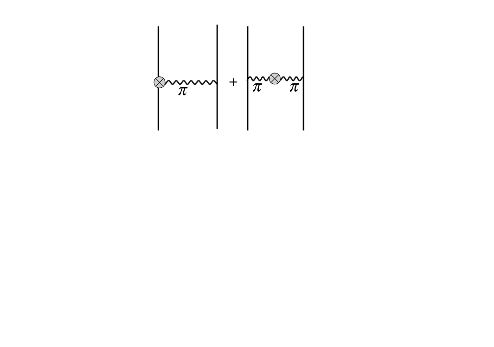
Figure 9: The leading “soft-pion” graphs contributing to exchange electromagnetic currents ([left] and [right]) and to exchange axial charge ([left]). The circled cross stands for the vector current $V^{\mu}$ or the axial current $A^{\mu}$. The propagators are as defined in Fig. 7.

We should emphasize that there are no heavy-meson or multi-pion exchanges at this order, a situation that renders the calculation for currents markedly simpler than for forces. What this means is that when massive degrees of freedom are explicitly included, they can contribute only at $O(Q^{2})$ relative to the tree order. Put more precisely, if one includes one soft-pion ($A_{\pi}$), two or more pion ($A_{\pi\pi}$) and vector meson ($A_{V}$) exchanges, excited baryons ($A_{N^{*}}$) and appropriate form factors ($A_{FF}$) as one customarily does in exchange current calculations, consistency with chiral symmetry requires that even though each contribution could be large, the sum must satisfy[99]

$$A_{\pi}+A_{\pi\pi}+A_{V}+A_{N^{*}}+A_{FF}\approx A_{\pi}(1+O(Q^{2})).$$ (III.94)

Later we will give a simple justification of this result by one-loop chiral perturbation theory and give a numerical value for the $O(Q^{2})$ term. The surprising thing is that the relation (III.94) holds remarkably well for the famous threshold electrodisintegration of the deuteron as well as in the magnetic form factors of ³He and ³H to large momentum transfers [110]. In the case of nuclear axial-charge transitions mediated by the time component of the isovector axial current which will be discussed below, one can construct a phenomenological model that fits nucleon-nucleon interactions which satisfies this condition well with the $O(Q^{2})$ less than 10% of the dominant soft-pion contribution.

3.5.3 Axial-charge transitions in nuclei

We now illustrate how our formalism works by applying it to what is known as axial-charge transition in nuclei. It involves the time component of the isovector axial current $\vec{J}_{5}^{\mu\pm}$ inducing the transition $0^{+}\leftrightarrow 0^{-}$ with $\Delta I=1$. This transition in heavy nuclei is quite sensitive to the soft-pion exchange as well as to the scaling effect[112] and illustrates nicely the power of chiral symmetry in understanding subtle nuclear phenomena.

Tree order

The axial-charge transition is described by a one-body (“impulse”) axial-charge operator plus a two-body (“exchange”) axial-charge operator described above. Three-body and higher many-body operators do not contribute at small energy-momentum transfer we will focus on. In a work done some time ago[111], these operators were calculated without the scaling effect. Now from the foregoing discussion, it is obvious that we will get the operators of exactly the same form except that the masses $m_{i}$’s are replaced by $m_{i}^{*}$’s and the coupling constants $g_{i}$’s are replaced by $g_{i}^{*}$’s. This means that in the results obtained previously, we are to make the following replacements

$$m_{N}\rightarrow m_{N}\Phi(\rho),\ \ \ \ f_{\pi}\rightarrow f_{\pi}\Phi,\ \ \ \ m_{\pi}\rightarrow m_{\pi}\sqrt{\Phi}$$ (III.95)

with $\Phi$ a density-dependent constant to be determined empirically. (This quantity is probably calculable from a microscopic Hamiltonian, but for the moment we should simply take it as a parameter.) At the mean-field level, the coupling constants $g_{\pi NN}$ and $g_{A}$ are not affected by density as shown above (see Eq.(III.80). We shall come back to loop effects later. The axial-charge density one-body and two-body operators are of the form

$$J_{5}^{0\pm} = J_{5}^{(1)\pm}+J_{5}^{(2)\pm},$$ (III.96)

$$J_{5}^{(1)\pm} = -g_{A}\sum_{i}\tau_{i}^{\pm}(\vec{\sigma}_{i}\cdot\vec{p}_{i}/m_{N}^{\star})\delta(\vec{x}-\vec{x}_{i}),$$ (III.97)

$$J_{5}^{(2)\pm} = \frac{{m_{\pi}^{\star}}^{2}}{8\pi f_{\pi}^{\star}}\left(\frac{g_{A}^{\star}}{f_{\pi}^{\star}}\right)\sum_{i<j}(\tau_{i}\times\tau_{j})^{\pm}[\vec{\sigma}_{i}\cdot\hat{r}\delta(\vec{x}-\vec{x}_{j})+\vec{\sigma}_{j}\cdot\hat{r}\delta(\vec{x}-\vec{x}_{i})]Z(r_{ij})$$ (III.98)

with

$$Z(r)=\left(1+\frac{1}{{m_{\pi}^{\star}}r}\right)e^{-{m_{\pi}^{\star}}r}/{m_{\pi}^{\star}}r$$

where $r_{ij}=\vec{x}_{i}-\vec{x}_{j}$ and $\vec{p}$ the initial momentum of the nucleon making the transition. The two-body current comes only from the left graph of Fig.9. We have set the current momentum equal to zero. Note that the star is put on all the quantities that scale within the framework given above. However in applying the result to actual transitions in nuclei, there is a subtlety due to the fact that the Gamow-Teller coupling constant $g_{A}$ scales in medium due to short-range interactions between baryons as described later. As a consequence, effectively, at least up to nuclear matter density, the constant $g_{A}^{\star}/f_{\pi}^{\star}$ associated with a pion exchange remains unscaled. Furthermore consideration based on QCD indicates that the properties of Goldstone bosons are not affected by the changes in the quark condensates. Thus we should take in Eq. (III.98) $m_{\pi}^{\star}\approx m_{\pi}$ and $\frac{g_{A}^{\star}}{f_{\pi}^{\star}}\approx\frac{g_{A}}{f_{\pi}}$. The $g_{A}$ that figures in the single-particle axial charge operator in (III.98) remains unscaled since it is not associated with a Gamow-Teller operator.

Let us denote the one-body matrix element calculated with the scaling by ${\cal M}_{1}^{*}$ and the corresponding two-body exchange current matrix element by ${\cal M}_{2}^{*}$

$${\cal M}^{*}_{a}\equiv\langle f|J_{5}^{(a)\pm}|i\rangle,\ \ \ \ a=1,2.$$ (III.99)

Let ${\cal M}_{a}$ denote the quantities calculated with the operators in which no scaling is taken into account. For comparison with experiments, it is a common practice to consider the ratio

$$\epsilon_{MEC}\equiv\frac{{\cal M}^{observed}}{{\cal M}_{1}}.$$ (III.100)

This is a ratio of an experimental quantity over a theoretical quantity, describing the deviation of the impulse approximation from the observation. The prediction that the present theory makes is remarkably simple. It is immediate from (III.96) and the argument given above that

$$\epsilon_{MEC}^{th}=\frac{{\cal M}_{1}^{*}+{\cal M}_{2}^{*}}{{\cal M}_{1}}=\Phi^{-1}(1+R)$$ (III.101)

where $R={\cal M}_{2}/{\cal M}_{1}$.

One-loop corrections

There are two ways of computing the $O(Q^{2})$ correction in (III.94). One is to introduce vector mesons and saturate the correction by tree graphs and the other is to compute one loop graphs with pions. Clearly the former is easier. However tree graphs with vector mesons are not complete as we know from $O(\partial^{4})$ in $\pi\pi$ scattering. There are nonanalytic terms coming from pion loops in addition to the counter terms saturated by the vectors. In this subsection, we shall compute the $O(Q^{2})$ correction to $R$ using pions and nucleons only. The $\Delta$ resonance does not contribute and the effect of the vector mesons $\rho$ and $a_{1}$ are effectively included in the treatment through the loop effect. These are discussed in the work of Park et al [100].

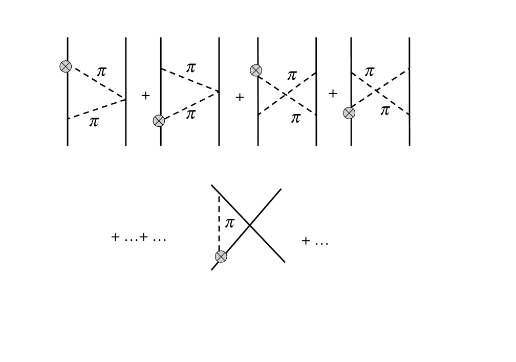
Figure 10: Two-body exchange graphs of $O(Q^{2})$ relative to the leading soft-pion graphs. The non-vanishing graphs are [a], [b] and [c]; all the rest, most of which are not shown here, do not contribute to the order considered. The dashed line represents the time-order pion propagator.

Let the corrected ratio be

$$R\rightarrow(1+\Delta)R$$ (III.102)

where $\Delta$ is given by the loops according to the counting rule given in (III.38). $\Delta$ can come from two sources. One is the loop correction to the soft-pion term of Fig. 9, essentially given by one-loop corrections to the vertex $A_{0}NN\pi$ since there is no one-loop correction in HFF to the $\pi NN$ vertex other than renormalizing the $\pi NN$ coupling constant $g_{\pi NN}$. Now the one-loop correction to the $A_{0}NN\pi$ is nothing but the one-loop correction to the isovector Dirac form factor $F_{1}^{V}$, so it is completely determined by experiments. We will call the corresponding correction $\Delta_{1\pi}$. The other class of diagrams contributing to $\Delta_{2\pi}$ is two-pion exchange graphs given in Figure 10. There are many other graphs one can draw but they do not contribute to the order considered when the HFF is used. In particular the four-fermion contact interactions that appear in nuclear forces do not play any role in the currents. In evaluating these graphs, Fig. 10, counter terms (there are effectively two of them) involving four-fermion field with derivatives are needed to remove divergences. They would also contribute to nuclear forces at the same chiral order. Now the finite counter terms that appear are the so-called “irrelevant terms” in effective theory (as they are down by the inverse power of the chiral scale parameter) and can only be probed at very short distance. Indeed the currents that come from such terms are $\delta$ functions and derivatives of the $\delta$ functions, so they should be suppressed if the wave functions have short-range correlations. Therefore the counter terms that appear here can be ignored. This can be also understood by the fact that such terms do not figure in phenomenological potentials; this also means that one cannot extract them from nucleon-nucleon scattering data. They could perhaps be seen if one measures small effects at very short distances. Thus embedded in nuclear medium, the unknown counter terms do not play any role. This is the part of “chiral filtering” by nuclear matter of short-wavelength degrees of freedom. A corollary to this “theorem” is that if the dominant soft-pion contribution is suppressed by kinematics or by selection rules, then the next order terms including $1/m_{N}$ corrections must enter. This is the other side of the same coin as predicted a long ago [111]. For instance, s-wave pion production in

$$pp\rightarrow pp\pi^{0}$$ (III.103)

is closely related to the matrix element of the axial charge operator. But because of an isospin selection rule, the soft-pion exchange current cannot contribute. Since the single-particle matrix element is kinematically suppressed, the contribution from higher chiral corrections will be substantial. This turns out to be the case [113]. The case with the space component of the axial current, namely, the coupling constant $g_{A}$ in nuclei, is discussed below.

Apart from these counter terms which are rendered ineffective inside nuclei, there are no unknown parameters once the masses of the nucleon and the pion and constants such as $g_{A}$, $f_{\pi}$ are taken from free space. We quote the results, omitting details. The quantity we want is the ratio of nuclear matrix elements (denoted by $<$ $>$)

$$\Delta_{1\pi} = \langle\delta J_{5}^{(2)}(1\pi)\rangle/\langle J_{5}^{(2)}(soft)\rangle,$$ (III.104)

$$\Delta_{2\pi} = \langle\delta J_{5}^{(2)}(2\pi)\rangle/\langle J_{5}^{(2)}(soft)\rangle$$ (III.105)

where $J_{5}^{(2)}(soft)$ is given by the soft-pion term (III.98)

$$J_{5}^{(2)}(soft)={\cal T}^{(1)}\frac{d}{dr}\left[-\frac{1}{4\pi r}e^{-m_{\pi}r}\right],$$ (III.106)

with the matrix element to be evaluated in the sense of (III.99) and

$$\delta J_{5}^{(2)}(1\pi) = \frac{m_{\pi}^{2}}{6}\langle r^{2}\rangle_{1}^{V}\frac{m_{\pi}^{2}}{f_{\pi}^{2}}\,J_{5}^{(2)}(soft)$$

$$+ \frac{{\cal T}^{(1)}}{16\pi^{2}f_{\pi}^{2}}\frac{d}{dr}\left\{-\frac{1+3g_{A}^{2}}{2}\left[K_{0}(r)-{\tilde{K}_{0}}(r)\right]+(2+4g_{A}^{2})\left[K_{2}(r)-{\tilde{K}_{2}}(r)\right]\right\},$$

$$\delta J_{5}^{(2)}(2\pi) = \frac{1}{16\pi^{2}f_{\pi}^{2}}\frac{d}{dr}\left\{-\left[\frac{3g_{A}^{2}-2}{4}K_{0}(r)+\frac{1}{2}g_{A}^{2}K_{1}(r)\right]{\cal T}^{(1)}+2g_{A}^{2}K_{0}(r){\cal T}^{(2)}\right\},$$

where $n\pi$ in the argument of the $\delta J_{5}$’s stands for $n\pi$ exchange in the one-loop graphs and $\langle r^{2}\rangle_{1}^{V}$ is the isovector charge radius of the nucleon. We have used the notations

$${\cal T}^{(1)} \equiv {\vec{\tau}}_{1}\times{\vec{\tau}}_{2}\,{\hat{r}}\cdot({\vec{\sigma}_{1}}+{\vec{\sigma}_{2}}),$$ (III.109)

$${\cal T}^{(2)} \equiv ({\vec{\tau}}_{1}+{\vec{\tau}}_{2})\,{\hat{r}}\cdot{\vec{\sigma}_{1}}\times{\vec{\sigma}_{2}}$$ (III.110)

and the functions $K_{i}$ and $\tilde{K}_{i}$ defined by

$$K_{0}(r) = -\frac{1}{4\pi r}\,\int_{0}^{1}dx\,\frac{2x^{2}}{1-x^{2}}\,E^{2}e^{-Er},$$

$$K_{2}(r) = -\frac{1}{4\pi r}\,\int_{0}^{1}dx\,\frac{2x^{2}}{1-x^{2}}\,\left(\frac{1}{4}-\frac{x^{2}}{12}\right)\,E^{2}e^{-Er}$$ (III.111)

and

$${\tilde{K}}_{0}(r) = \frac{1}{4\pi r}\,\int_{0}^{1}dx\,\frac{2x^{2}}{1-x^{2}}\,\frac{m_{\pi}^{2}}{m_{\pi}^{2}-E^{2}}\,\left(m_{\pi}^{2}e^{-m_{\pi}r}-E^{2}e^{-Er}\right),$$

$${\tilde{K}}_{2}(r) = \frac{1}{4\pi r}\,\int_{0}^{1}dx\,\frac{2x^{2}}{1-x^{2}}\,\left(\frac{1}{4}-\frac{x^{2}}{12}\right)\,\frac{m_{\pi}^{2}}{m_{\pi}^{2}-E^{2}}\,\left(m_{\pi}^{2}e^{-m_{\pi}r}-E^{2}e^{-Er}\right).$$ (III.112)

Here $E(x)=2m_{\pi}/\sqrt{1-x^{2}}$. These are Fourier-transforms of McDonald functions and their derivatives with $\delta$ function terms excised on account of short-range correlations.

For a first estimate, we shall calculate the relevant matrix elements in fermi-gas model with a short-range correlation function in the simple form (in coordinate space)

$$g(r)=\theta(r-d),\ \ \ r=|\vec{r}_{1}-\vec{r}_{2}|.$$ (III.113)

Figure 11 summarizes the result for various short-range cut-off $d$. The relevant $d$ commonly used in the literature is 0.7 fm. It is difficult to pin down the cut-off accurately but this is roughly what realistic calculations give.

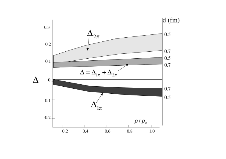
Figure 11: The $O(Q^{2})$ correction $\Delta_{1\pi}$, $\Delta_{2\pi}$ and $\Delta=\Delta_{1\pi}+\Delta_{2\pi}$ calculated in Fermi gas model as function of density $\rho/\rho_{0}$ for short-range cut-off $d=0.5$ fm and $0.7$ fm. The possible uncertainty in the value of cut-off is indicated by the shaded area.

Numerically although $\Delta_{1\pi}$ and $\Delta_{2\pi}$ can be non-negligible individually, there is a large cancellation, so the total is small, $\Delta<0.1$. This is the chiral filter mechanism mentioned before. This cancellation mechanism which is also operative in nuclear electromagnetic processes mediated by magnetic operators as in the electrodisintegration of the deuteron and the magnetic form factors of the tri-nucleon systems is characteristic of the strong constraints coming from chiral symmetry, analogous to the pair suppression in $\pi$N scattering.

Absence of multi-body currents

For small energy transfer (say, much less than $m_{\pi}$), three-body and other multi-body forces do not contribute to $O(Q^{2})$ relative to the soft-pion term. This can be seen in the following way.

Consider attaching an axial-charge operator to the vertices in the graphs for three-body forces, Figure 12. We need not consider those graphs where the operator acts on any of the nucleon line. Now the argument that the sum of all such irreducible graphs cannot contribute to the order considered as long as the static pion propagator is used for two-body soft-pion exchange currents parallels exactly the argument used for the forces.

The situation is quite different, however, if the energy transfer is larger than say the pion mass as in the case where a $\Delta$ is excited by an external electroweak probe. In such cases, there is no reason why three-body and higher-body currents should be small compared with one- and two-body currents. This phenomenon should be measurable by high intensity electron machines at multi-GeV region.

Figure 12: Three-body currents suppressed to $O(Q^{2})$ relative to the soft-pion (two-body) graphs. The mechanism for the suppression is the same as for three-body forces to the same chiral order. As before, the wiggly line represents the Feynman propagator and the dotted line the time-ordered propagator of the pion.

Comparison with experiments

We shall estimate the ratio $R$ in fermi-gas model. This will give us a global estimate. It turns out that the ratio $R$ depends little on nuclear model and on mass number. In fermi-gas model, it is given by

$$R=\frac{g_{\pi NN}^{2}}{4\pi^{2}g_{A}^{2}}\frac{p_{F}}{m_{N}}\left[1+\lambda-\lambda(1+\frac{\lambda}{2})\ln(1+\frac{2}{\lambda})\right]$$ (III.114)

with $\lambda\equiv\frac{m_{\pi}^{2}}{2p_{F}^{2}}$, where $p_{F}$ is the Fermi momentum (which is $(\frac{3\pi^{2}}{2}\rho)^{1/3}$ for nuclear matter). Numerically this ranges from $R\approx 0.44$ for $\rho=\frac{1}{2}\rho_{0}$ to $R\approx 0.62$ for $\rho=\rho_{0}$. Now in the same model with a reasonable short-range correlation, $\Delta$ comes out to be about 0.1, pretty much independently of nuclear density[100], so that we can take

$$R(1+\Delta)\approx 1.1R.$$ (III.115)

The only undetermined parameter in this theory is the scaling factor $\Phi$. Ideally one should determine it from experiments. However it is a mean-field quantity which makes sense only for large nuclei and has not been pinned down yet. Once it is fixed in heavy nuclei, one could then use local-density approximation to describe transitions in light nuclei. At the moment it is known only from QCD sum-rule calculations of hadrons in medium, e.g., the vector-meson mass [114]. To have a qualitative idea, we shall take

$$\Phi\approx 1-0.18\frac{\rho}{\rho_{0}}.$$ (III.116)

With eqs. (III.115) and (III.116), we predict

$$\epsilon_{MEC} \approx 1.63,\,2.05\,\ \ {\rm for}\ \rho=\rho_{0}/2,\,\rho_{0}.$$ (III.117)

In view of the crudeness in (III.115) we have an uncertainty of $\pm 0.2$ in these values. This agrees with the result (experimentally $\approx 1.6$) in light nuclei as well as with the results (experimentally $\sim 2$) in heavy nuclei[115]. The empirical value in the Pb region is

$$\epsilon_{MEC}^{exp}=2.01\pm 0.05.$$ (III.118)

For a meaningful test of the theory, a finite-nucleus calculation will be required.

3.5.4 $g_{A}^{*}$ in Nuclei

As already discussed, at the tree level of the effective Lagrangian, the axial-vector coupling constant $g_{A}$ is not renormalized in medium. Here we illustrate how short-distance in-medium effects which cannot be included by low-order chiral perturbation theory can induce an important density dependence for the Gamow-Teller vertex. Such a correction is actually required by the observation that the value of $g_{A}$ measured in the neutron beta decay [116]

$$g_{A}=1.262\pm 0.005$$ (III.119)

is quenched to about 1 in medium and heavy nuclei[117]. This explains why we must take $g_{A}^{\star}/f_{\pi}^{\star}\approx g_{A}/f_{\pi}$ for the $\pi NN$ vertex contributing to the one-pion exchange operators, at least up to nuclear matter density. The important point here is that this quenching is not to be attributed to an influence of a modified vacuum, in other words, a “fundamental quenching” as often thought in the past. This is obviated by the fact that in large $N_{c}$ QCD, it is the $O(1/N_{c}^{2})$ correction that is affected by nuclear medium. Of course at an asymptotic density, $g_{A}$ should reach unity as a consequence of the melting of the quark condensate.

In nuclei, $g_{A}^{*}$ is measured in Gamow-Teller transitions, namely the space component of the axial current. For this component, the exchange current given by the soft-pion theorem discussed above is suppressed. Therefore according the corollary to the “chiral filter” argument, corrections to $g_{A}^{*}$ must come from loop terms and/or higher $Q$ Lagrangian pieces or many-body currents involving short-distance physics . It is known that the dominant correction comes from the excitation of $\Delta$-hole states as given in Fig. 13.

Figure 13: The $\Delta$-hole graph involving four-baryon contact interaction that plays a dominant role in quenching $g_{A}$ in nuclei. The cross stands for $\vec{A}$,the space component of the axial current, the double line stands for the $\Delta$ and $N^{-1}$ for the nucleon hole.

The introduction of the $\Delta$ requires extending the effective Lagrangian to decuplet (spin-3/2) baryons in the case of three flavors. This can be done in the following way[118].

Introduce a Rarita-Schwinger field $\Delta^{\mu}$ obeying the constraint $\gamma_{\mu}\Delta^{\mu}=0$. This field carries $SU(3)$ tensor indices $abc$ that are completely symmetrized to form the decuplet. The chirally symmetric Lagrangian involving the decuplet with its coupling to octet baryon and mesons equivalent to (III.16) is

$${\cal L}^{\Delta}=i\bar{\Delta^{\mu}}\gamma_{\nu}{\cal D}^{\nu}\Delta_{\mu}-m_{\Delta}\bar{\Delta}^{\mu}\Delta_{\mu}+\alpha\left(\bar{\Delta}^{\mu}A_{\mu}B+h.c.\right)+\beta\bar{\Delta}^{\mu}\gamma_{\nu}\gamma_{5}A^{\nu}\Delta_{\mu},$$ (III.120)

where $\alpha$ and $\beta$ are unknown constants, $B$ stands for the spin-1/2 octet baryons, $\Delta^{\mu}$ the spin-3/2 decuplets $\Delta$, $\Sigma^{*}$, $\Xi^{*}$ and $\Omega$ and $A^{\mu}$ is the “induced” axial vector $A^{\mu}=\frac{i}{2}(\xi\partial^{\mu}\xi^{\dagger}-\xi^{\dagger}\partial^{\mu}\xi)$. Sum over all $SU(3)$ indices (not explicitly written down here) is understood. The covariant derivative acting on the Rarita-Schwinger field is defined by

$${\cal D}^{\nu}\Delta^{\mu}_{abc}=\partial^{\nu}\Delta^{\mu}_{abc}+(V^{\nu})^{d}_{a}\Delta^{\mu}_{dbc}+(V^{\mu})^{d}_{b}\Delta^{\mu}_{adc}+(V^{\mu})^{d}_{c}\Delta^{\mu}_{abd}$$ (III.121)

with $V^{\mu}=\frac{1}{2}(\xi\partial^{\mu}\xi^{\dagger}+\xi^{\dagger}\partial^{\mu}\xi)$. Under chiral $SU_{L}(3)\times SU_{R}(3)$ transformation, the Rarita-Schwinger field transforms as

$$\Delta^{\mu}_{abc}\rightarrow g^{d}_{a}g^{e}_{b}g^{f}_{c}\Delta^{\mu}_{def}.$$ (III.122)

As before, we have terms quadratic in baryon fields which we may write

$${\cal L}^{\Delta}_{4}=\gamma\left(\bar{\Delta}^{\mu}{\cal C}_{\mu\nu}B\bar{B}{\cal F}^{\nu}B+h.c.\right)+(\Delta\Delta BB)+(\Delta B\Delta B)+(\Delta\Delta\Delta\Delta)+\cdots.$$ (III.123)

where ${\cal C}$ and ${\cal F}$ are appropriate tensors allowed by Lorentz and isospin invariance. We have indicated explicitly only the $\Delta BBB$ components as they play the essential role for $g_{A}^{*}$.

As with the nucleon, we can use the heavy-baryon formalism for the $\Delta$. Evaluating the diagram in Fig.III.9 requires information on the axial-vector coupling constant $g_{A}^{\Delta}$ connecting to $\Delta$ and $N$ and the contact interaction $g_{\Delta}^{\prime}$ for $\Delta N\leftrightarrow NN$ in the particle-hole channel. The latter is analogous to the Landau-Migdal particle-hole interaction $g_{0}^{\prime}\vec{\tau}_{1}\cdot\vec{\tau}_{2}\vec{\sigma}_{1}\cdot\vec{\sigma}_{2}\delta(r_{12})$ governing spin-isospin interactions in nuclei and can be written in terms of the transition spin operator $\vec{S}$ and transition isospin operator $\vec{T}$ as[119]

$$g_{\Delta}^{\prime}\vec{T}_{1}\cdot\vec{\tau}_{2}\vec{S}_{1}\cdot\vec{\sigma}_{2}\delta(r_{12}).$$ (III.124)

Neither ${g_{A}^{\Delta}}$ nor $g_{\Delta}^{\prime}$ is known sufficiently well. Assuming that the axial-vector current couples to the $\Delta$ and $N$ in the same way as the pion does, one usually takes

$$g_{A}^{\Delta}/g_{A}\approx 2.$$ (III.125)

We can then roughly estimate in small-density approximation that

$$g_{A}^{*}/g_{A}=1-ag_{\Delta}^{\prime}\rho(m_{\Delta}-m_{N})^{-1}+\cdots$$ (III.126)

with $a\approx(\frac{2}{3}{m_{\pi}}^{-1})^{2}$ (where the factor $(2/3)$ comes from the matrix element of the transition spin and isospin). It turns out that the acceptable empirical value (coming from pion-nucleus scattering) for $g_{\Delta}^{\prime}$ is about $1/3$. Taking the $\Delta N$ mass difference $\sim 2.1m_{\pi}$, we have

$$g_{A}^{*}/g_{A}\approx 0.8\ \ \ {\rm for}\ \ \rho=\rho_{0}.$$ (III.127)

This makes $g_{A}^{*}$ approximately 1 in nuclear matter.

There are many other diagrams contributing at the same order but none of them is as important as Fig.V.9 except possibly for core polarizations involving particle-hole excitations through tensor interactions . What one observes in nuclei is of course the sum of all. The point of the above exercise is that the $g_{A}$ is quenched in nuclei due to higher order chiral effects of short-range character and not due to soft pions.

3.6 Nuclei in the “Swelled World”

The case of axial-charge transitions (and the isovector magnetic dipole process which we did not discuss here) corresponds to small energy and momentum transfers $q_{\mu}\approx 0$. The effective Lagrangian (III.76) with the parameters scaled as

$$\frac{m_{B}^{*}}{m_{B}}\approx\frac{m_{V}^{*}}{m_{V}}\approx\frac{m_{\sigma}^{*}}{m_{\sigma}}\approx\frac{f_{\pi}^{*}}{f_{\pi}}\equiv\Phi(\rho)$$ (III.128)

can be applied to other nuclear processes of similar nature. For this relation to be useful, it is necessary that the process studied should be dominated by tree graphs, with next chiral order corrections suppressed as in the axial-charge example seen above. In phenomenological approach in nuclear physics, this is usually the case. Let us therefore consider cases where the scaling (III.128) makes a marked improvement in fitting experimental data. Here we discuss a few of such examples [120].

3.6.1 Tensor forces in nuclei

If the $\rho$ field is not integrated out assuming that its mass is very high, then at tree level, there can be two terms contributing to tensor forces in nuclei. The first is the tensor force coming from one-pion exchange. As noted before, there is little scaling in the one-pion exchange potential, so this part will be left untouched by medium. The second is a contribution from one-$\rho$ exchange and this part will be scaled. As we saw before, the vector mesons contribute to forces at the same chiral order as the pion. Effectively the tensor force has the form

$$V_{T}(\vec{q},\omega)= - \frac{f^{2}}{m_{\pi}^{2}}\left[\frac{\vec{\sigma}_{1}\cdot\vec{q}\vec{\sigma}_{2}\cdot\vec{q}-\frac{1}{3}(\vec{\sigma}_{1}\cdot\vec{\sigma}_{2})q^{2}}{(q^{2}+m_{\pi}^{2})-\omega^{2}}\right]{\bf\tau}_{1}\cdot{\bf\tau}_{2}$$ (III.129)

$$+ \frac{{f^{*}_{\rho}}^{2}}{{m^{*}_{\rho}}^{2}}\left[\frac{\vec{\sigma}_{1}\cdot\vec{q}\vec{\sigma}_{2}\cdot\vec{q}-\frac{1}{3}(\vec{\sigma}_{1}\cdot\vec{\sigma}_{2})q^{2}}{(q^{2}+{m^{*}_{\rho}}^{2})-\omega^{2}}\right]{\bf\tau}_{1}\cdot{\bf\tau}_{2}$$

where we have defined $\frac{f^{2}}{m_{\pi}^{2}}=\left(\frac{g_{A}}{2f_{\pi}}\right)^{2}$. It is assumed in (III.129) that the pion-exchange term is unscaled up to nuclear matter density as suggested by nature. Using

$$\frac{{f^{*}_{\rho}}^{2}}{{m^{*}_{\rho}}^{2}}\approx\frac{{f_{\rho}}^{2}}{{m_{\rho}}^{2}}\Phi(\rho)^{-2}$$ (III.130)

and the empirical observation

$$\frac{{f_{\rho}}^{2}}{{m_{\rho}}^{2}}\approx 2\frac{f^{2}}{{m_{\pi}}^{2}}$$ (III.131)

we see that the tensor force would vanish when

$$\frac{1}{2}\Phi^{2}\frac{\langle(q^{2}+{m^{*}_{\rho}}^{2})\rangle}{\langle(q^{2}+m_{\pi}^{2})\rangle}\approx 1$$ (III.132)

where we have set $\omega\approx 0$ for static force. This happens when $\langle q^{2}\rangle\approx 7.6m_{\pi}^{2}$ for $\Phi\approx 0.8$ corresponding to nuclear matter density. This is within the range of momentum a meson carries between nucleons in nuclear matter. Such effects of a medium-quenched tensor force are observed in $(e,e^{\prime})$ and $(p,p^{\prime})$ processes on heavy nuclei at several hundreds of MeV: The value of $\Phi$ required is $m^{*}/m=$ 0.79 – 0.86 which is consistent with the value needed to explain the enhanced axial charge transitions seen in Pb nuclei (see Eq. (III.116)). This again indicates that the $\rho$ should be considered on the same footing as the $\pi$ when nucleons are present. This is consistent with the picture of the $\rho$ as a light gauge field.

3.6.2 Other processes

Other evidences [122] are:

• Electroweak probes. In addition to the weak current discussed above, electromagnetic probes also provide an indirect evidence of the scaling effect. Specifically, the scaling of the vector meson and nucleon masses can be used to explain the longitudinal-to-transverse response function ratios in $(e,e^{\prime}p)$ processes with such nuclei as ³He, ⁴He and ⁴⁰Ca. Experimentally there is quenching in the longitudinal response function that seems to increase with nuclear density while the transverse response remains unaffected. This feature can be economically (but perhaps not uniquely) explained by the scaling vector meson masses.

• Hadronic probes. Some long-standing problems in hadron-nucleus scattering (i.e, the kaon-nucleus and nucleon-nucleus optical potentials) are resolved by a quenched vector-meson mass. A stiffening of nucleon-nucleus spin-isospin response is predicted and is observed. These effects are manifested through the forces mediating the processes and the change in the range of such forces due to the scaling masses.

3.7 Appendix Added 1: Effective Field Theory for Nuclei

During slightly more than one decade since Weinberg’s paper in 1990 [97], there has been a splurge of activity in applying effective field theory to the studies of two-nucleon systems, principally of two-nucleon scattering and two-nucleon potential and less of few-nucleon response functions. Here the focus has been to assess how well one can understand nucleon-nucleon dynamics from the starting point of an effective theory anchored on “fundamental principles,” namely QCD. Although there have been efforts to address three- or more-body systems for a similar purpose, there has been little progress on them. The up-to-date status of the progress made so far was reviewed in [144]. Leaving this part of the story to the review article and references given therein, I would like to summarize an aspect of nuclear EFT that is of a different objective than just “seeing” how EFT works in nuclei and how much one can reproduce what has been achieved by the standard nuclear physics approach (SNPA) [145]. If nuclear EFT is to be a reliable representation of QCD in nuclei, then it must have the power of predictiveness that the SNPA – which is anchored largely on phenomenology – cannot achieve. What I would like to do here is to describe what EFT has been able to do in making predictions that cannot be done otherwise for processes that figure importantly in astrophysics. The point I emphasize here is that one should recognize that the “old” SNPA is not an object alien to the basic theory of strong interactions but rather is an integral – though perhaps incomplete – part of it and an EFT that incorporates the SNPA in a way consistent with the tenet of EFT is a lot more powerful than one which eschews the SNPA. This aspect has been largely enunciated in several recent publications [136, 146].

3.7.1 Chiral filter mechanism

In contrast to the approaches adhering to strict order-by-order power counting rule proposed subsequently to Weinberg’s work [97], I find it a lot more powerful for my purpose to follow Weinberg’s original chiral perturbation scheme in which the pion exchange is put on the same footing as contact non-derivative four-nucleon interactions with the pion mass incorporated by means of perturbative unitarity. This is because it allows a direct contact with the SNPA and the wealth of information available from the long history of nuclear physics. There is a bit of problem with the power counting when the pion is present ab initio and this has been discussed extensively by several people [144]. I would not like to get into that matter as I believe it is a technical matter that does not seem to be important in most of the processes considered so far.

I will take it for granted that a sophisticated phenomenology with light nuclei can supply us accurate wave functions with which one can calculate response functions. Although $n$-body potentials for $n>2$ cannot be unambiguously determined in this way, two-body and possibly three-body potentials could be determined with great accuracy. And there is a growing evidence that this is the case. Solving the Schrödinger equation with such potentials corresponds to summing to all orders a subset of “reducible graphs” in the EFT expansion, with the “irreducible graphs” subsumed to be taken into account in the “accurate potentials” up to some high order. In exploiting these accurate wave functions that emerge from such calculations in the context of an EFT, it would of course be highly desirable to have a clear idea what is included and what is not in the potentials used. In some cases, one of which is discussed here, this is possible. Now given such wave functions, can one calculate response functions measured in precision experiments as accurately as possible with the possibility of controlling the theoretical errors one commits ? This question can be answered affirmatively for the calculation of responses to slowly-varying EW fields.

Consider the matrix element of the vector current $J_{\mu}^{a}$ and the axial-vector current $J_{5\mu}^{a}$. We are interested in calculating $\langle f|J_{\mu}|i\rangle$ where $i$ and $f$ denote respectively the initial and final nuclear states. This current effective in an $A$-body system can be decomposed into

$$J_{\mu}=\sum_{n=1}^{A}J_{\mu}^{(n)}.$$ (III.133)

Customarily, except for unusual cases, an example of which we will encounter below, one-body terms are leading in the power counting (chiral counting in chiral-invariant theories) – and they $are$ leading numerically, so the theorist’s task is to compute the matrix elements of higher-body currents. Since the EW current will act only once for very weak and slowly-varying interactions, it suffices to systematically count the chiral orders of the irreducible graphs contributing to the current. This strategy is rather close to the that initiated many years ago [109]. In terms of exchanges of mesons between the nucleons in interaction, the dominant “correction” to the leading one-body is the 2-body contribution with the exchange of one soft-pion. Recall that the chiral filter mechanism states [111] that whenever the one soft-pion exchange is allowed, unsuppressed by kinematics and symmetry, the soft-pion-exchange two-body current dominates the correction with higher (chiral order) terms suppressed typically by an order of magnitude and yet calculable reliably. This means that one can compute the transition matrix elements with high accuracy within the framework of chiral perturbation theory. Conversely if the one-soft-pion term is suppressed, then corrections to the leading term are several orders higher in the power counting or shorter-ranged and cannot be accessed reliably with only a finite number of terms. In this case, ordinary chiral perturbation theory is not much of power and one has to resort to a different strategy than ordinary chiral perturbation theory. A simple analysis of the graphs of Fig. 9 shows that the space component of the vector current and the time component of the axial current are protected by the chiral filter mechanism and the remainders are not [111]. One beautiful example that supports this observation is the thermal $np$ capture process [147] which involves the space component of the vector current, that is, the isovector $M1$ operator,

$$n+p\rightarrow d+\gamma,$$ (III.134)

the cross section of which is predicted (in the sense that there are no free parameters) with a theoretical error of $\mathrel{\raise 1.29167pt\hbox{$<$\kern-7.5pt\lower 4.30554pt\hbox{$\sim$}}}1\%$ with the prediction agreeing perfectly with the experiment. The other example is the axial charge transition in heavy nuclei

$$A(0^{\pm})\rightarrow A^{\prime}(0^{\mp})\ e\ \nu\ \ \ \Delta T=1.$$ (III.135)

It has been confirmed in forbidden $\beta$ transitions that the enhancement due to the soft-pion exchange graph with a suitable scaling due to density in the chiral Lagrangian (described below) can be $\sim 100\%$ in heavy nuclei such as Pb [112, 148, 149].

3.7.2 Predictions for the solar $pp$ and $hep$ processes

It turns out, somewhat unexpectedly, that even when the chiral filter mechanism is suppressed and hence the soft-pion contribution is absent, under certain circumstances (to be described below), one can still make accurate predictions without being obstructed by unknown parameters. I discuss two cases here which are quite important for astrophysics.  The processes I will consider, recently discussed in [150, 151], are

$$p+p \rightarrow d+e^{+}+\nu_{e},$$ (III.136)

$${}^{3}{\rm He}+p \rightarrow {}^{4}{\rm He}+e^{+}+\nu_{e}.$$ (III.137)

These two processes are important for the solar neutrino problem that has bearing on the issues of neutrino mass and stellar evolution. What we are concerned with here is neither the neutrino mass nor the stellar evolution but with the strong interaction input – that is, accurate nuclear matrix elements of the weak current – which is of course essential for the main issues. This problem turns out to be highly nontrivial, particularly for the $hep$ process (III.137), for the following reasons. A naive (chiral) power counting shows that the dominant contribution should come from the space part of the axial current, in particular, the single-particle Gamow-Teller (GT) operator, since the lepton momentum transfer is small. However the chiral filter argument says that the soft-pion correction is suppressed for the space component of the axial current and hence corrections to the leading one-body current would inevitably involve shorter-distance physics. In terms of the chiral power counting relative to the leading single-particle GT operator which formally is of ${\cal O}(p^{0})$, corrections to the GT would start at next-to-next-to-next-to-leading order (denoted N³LO or ${\cal O}(p^{3})$). (There are also small contributions from the axial charge operator but this operator is protected by the chiral filter and hence is accurately calculable.) If the single-particle GT matrix element does not have an $anomalous$ suppression, then this term should make up the bulk of the amplitude and the N³LO correction, even with an inherent uncertainty, would not affect the total significantly. This is indeed the case for the $pp$ process (III.136): Here the single-particle term makes up typically more than 95 % of the decay rate. However this is not the case for (III.137) because of an “accidental” suppression of the single-particle GT term caused by the spatial symmetry mismatch between the initial and final wave functions. Furthermore the situation is even more acerbated since the leading correction term comes with an opposite sign to the single-particle term with a comparable magnitude. Due to the cancellation, the resulting decay rate could differ by orders of magnitude depending on the theory. Thus for the process in question, it is imperative that the suppressed correction term be calculated with high accuracy as emphasized in the context of EFT in [152].

The details of the solution to this problem are rather complex but the general idea of how it comes about is rather simple. I shall describe this in as simple a way as possible. Since other terms than the GT are straightforward and unambiguous, let me focus on the GT.

Since the long-range soft-pionic contribution is made inoperative in the GT channel, it is the short-range interaction that figures importantly. In the standard nuclear physics approach, this aspect of physics is interpreted as “short-range correlation.” In the present framework of EFT, this short-distance N³LO current receives contributions from both “hard” pionic part and heavy mesonic part, zero-ranged as the heavy mesons are integrated out. Denote the matrix element of the finite-range pionic part by

$$M_{\pi}=\int d^{3}rF_{\pi}(r)$$ (III.138)

and that of the zero-ranged pionic part and heavy-meson parts by

$$M_{zero}=\int d^{3}rF_{zero}(r).$$ (III.139)

The coefficients of the operators in (III.138) as well as the pionic part of (III.139) are of course known. However the rest of the terms in (III.139), such as, e.g., the counter terms, are not known. Since they must depend on the cutoff imposed, they cannot be obtained by saturating with a set of known heavy mesons. They can only be determined from experiments if data are available.

To have a contact with SNPA, we work in coordinate space. The quantities $F_{\pi,{zero}}(r)$ contain information on the “exact” wave functions (with the phenomenological potentials fitted to an ensemble of experimental data). By the procedure, the wave functions embody not only the physics ingredient that figures in the calculation of the currents calculated to N³LO but also much – though perhaps not all – of short-distance interactions that are of higher order than N³LO. If the currents were calculated to all orders in the chiral counting and the wave functions corresponded to the same order, then the integrals would be well-defined without any further regularization. However our currents are calculated to a given order, i.e., N³LO, and the wave function to an order presumably higher than N³LO. Therefore, the integrals will diverge and to make sense, an ultraviolet regularization is needed. In SNPA, one customarily cuts off the integral at a “hard-core” size $r=r_{c}$. Such a hard core kills all zero-range terms (including all counter terms) in (III.139) as well as cuts the short-range piece of the (known) finite-range terms in (III.138). I will call this SNPA procedure “hard-core regularization (HCR).” If the process is dominated by long-range interactions as in the case where the chiral filter mechanism is operative, this prescription is expected – and verified – to be reliable. The prime example is the thermal $np$ capture mentioned above. However in the present problem, the principal action comes from the short-distance part, so it is evident that the HCR prescription will give a result that strongly depends on the hard-core radius, thus upsetting the tenet of EFT and hence predictivity.

This is where the basic idea of EFT comes to help. The strategy of EFT is to regularize the operators in both (III.138) and (III.139) in such a way that the integrals be well-defined and the sum of (III.138) and (III.139) come out independent of the cutoff one imposes to the order considered . This regularization will be referred to as “modified hard-core regularization (MHCR).” This is not a trivial feat and there seems to be much misunderstanding on this in the community of nuclear EFT.

Now, what is the relevant scale of the cutoff? Since the lightest degrees of freedom that enter in the short-distance physics embedded in the counter terms are the scalar $\sigma$, $\rho$, $\omega$ mesons, we expect the cutoff to be in the vicinity of the $\sigma$ mass $\mathrel{\raise 1.29167pt\hbox{$>$\kern-7.5pt\lower 4.30554pt\hbox{$\sim$}}}500$ MeV.

Next what is expected of a bona-fide EFT? An EFT requires that the cutoff dependence in (III.138) – that reflects defect in short-distance physics in (III.138) – be cancelled by the cutoff dependence in (III.139). This implies that the coefficients of the counter terms will be cutoff dependent; the stronger it will be, the more short-ranged the physics is. Now in order for this procedure to work, we need an independent experimental source that determines the cut-off dependent parameters in (III.139). For the processes in question (III.136) and (III.137), it is the tritium beta decay that supplies the crucial link:

$${}^{3}{\rm H}\rightarrow^{3}{\rm He}+e^{-}+\bar{\nu}_{e}.$$ (III.140)

What turns out to be remarkable is that the same linear combination of counter-term operators figures in all three processes (III.136), (III.137) and (III.140). The reason for this “miracle” is that the same symmetry is operative in this GT channel. Furthermore since one is dealing with a rather short-ranged interaction, the same dynamics prevails for the two-body current whether it takes place in two-body, 3-body or 4-body systems. Thus once the single unknown term (called $\hat{d}^{R}$ in [150, 151]) is fixed for a given cutoff from (III.140), there are no free parameters for the processes (III.136) and (III.137). This makes the calculation of the delicate correction term firmer since three-body and four-body currents (suppressed by power counting) turn out to be totally negligible numerically.

To give an idea what happens, let me give what is called “S factor” which carries the nuclear information needed. With the error estimated from the cutoff dependence in the range $500\leq\Lambda/{\rm MeV}\leq 800$, the results are

$$S_{pp} = 3.94(1\pm 10^{-3})\times 10^{-25}\ {\rm MeV-barn},$$ (III.141)

$$S_{hep} = (8.5\pm 1.4)\times 10^{-20}\ {\rm MeV-barn}.$$ (III.142)

I would say that these results are one of the most accurate predictions ever made in nuclear physics. The reason why the $pp$ can be calculated with such a greater precision is that the main term is the single-particle GT and the correction term which is quite small $\mathrel{\raise 1.29167pt\hbox{$<$\kern-7.5pt\lower 4.30554pt\hbox{$\sim$}}}1$ % can be more or less controlled. Because of the accidental suppression of the single-particle GT, such an accuracy cannot be attained in the $hep$ process. Nonetheless, the result is remarkable, considering that in the past the uncertainty was orders of magnitude.

To conclude, whenever the chiral filter is operative, the dominant single-particle contribution and the soft-pion correction thereof are accurately given by the matrix elements computed with the SNPA wave functions. In this case, it is possible to argue that the wave functions do make an integral part of the EFT itself. The aficionados of the puristic power counting will agree to this statement since it is possible to do a rigorous calculation fully consistent with chiral counting at each order and come to the same result. But there is nothing really gained in adhering to the counting rule since one learns nothing beyond what we already know from SNPA. When the chiral filter mechanism is not operative, the same aficionados will face difficulty in calculating, say, the $hep$ process because it involves short distance and hence high orders, perhaps much higher than what can be managed with the given experimental data.

I should note that in the approach presented here, the possible error in counting brought in by the “exact” wave functions with ${\cal O}(p^{3})$ currents is most likely compensated by the regularization procedure that assures the cutoff independence. Exactly the same observation was made in the calculation of the isoscalar $M1$ and $E2$ matrix elements in the process $n+p\rightarrow d+\gamma$ [153]. Although these matrix elements, governed by the chiral-filter-unprotected operators, are suppressed with respect to the dominant isovector $M1$ matrix element by $\sim$ three orders of magnitude, the same regularization scheme used above produced a prediction with a very small theoretical error bar. What is in action is again a universal feature associated with the short-distance interaction not easily accessible by a low-order chiral perturbation expansion. This prediction can be potentially checked by experiments.

3.7.3 Experimental tests

There are a number of experimental indications that the predictions or postdictions for those processes protected by the chiral filter are valid. The situation for the predictions discussed above where a short-distance regularization, i.e., the modified hard-core regularization (MHCR), enters has not yet been confirmed. When the parity-violation experiments in the process $n+p\rightarrow d+\gamma$ are sufficiently refined, one could perhaps isolate the suppressed isoscalar $M1$ matrix element ($M1S$) and $E2$ matrix element ($E2S$) and check the prediction based on the MHCR. The presently available data on polarization observables are not precise enough for the test.

The solar neutrino experiments performed at the SNO and the super-Kamiokande provide some information on the $hep$ process but at present, there is little one can say about the value of the $hep$ amplitude from the observation. Future refined measurements will perhaps supply the necessary information.

A process somewhat related to the $hep$ process is the $``hen"$ process

$${}^{3}{\rm He}+n\rightarrow^{4}{\rm He}+\gamma$$ (III.143)

which involves the same wave function overlap problem. An EFT analysis using the same strategy used for the $hep$ process might be illuminating to test some of the ideas used for the latter. However one should note that as is known since a long time [109] the structure of multi-body currents is basically different between the EM vector current that enters in (III.143) and the axial-current that enters in (III.137). It is not obvious that the short-distance physics that plays a crucial role in (III.137) figures in (III.143) in the same way. This point is being analyzed and we will have the answer in the near future.

3.8 Appendix Added 2: Intrinsic Density Dependence of In-Medium Effective Chiral Lagrangians and Landau Fermi-Liquid Fixed Point Parameters

One of the most important developments in the field of effective field theories in many-hadron systems is the finding that matching to QCD of an effective theory with chiral symmetry leads to the notion that the $bare$ parameters of the Lagrangian defined at a scale $\bar{\Lambda}$ must have an intrinsic density dependence just as was found in BR scaling described in the ELAP 93 lecture. This story will be discussed in an appendix in the next section. Here I would like to discuss the possible relation found since 93 between the density-dependent parameters of the chiral Lagrangian to the Fermi-liquid fixed point parameters: This issue was briefly alluded to in Section 3.4 above.

3.8.1 Walecka mean field theory with intrinsic density dependence

We start with the ground state of many-body systems, in particular nuclear matter. In the next subsection, we will consider fluctuations.

For the ground state, we exploit the fact that Walecka’s mean field theory [123] is equivalent to Fermi-liquid theory [143]. To set up the EFT for the system, let us consider that the degrees of freedom we want to take into account explicitly, $\Phi_{L}$ of (III.43), now contain nucleons, pions and vector mesons. In fact the same can be formulated with the vector mesons and other heavy mesons integrated out but it is convenient to put the vectors and a scalar meson denoted $\phi$ explicitly. In free space this scalar may be the scalar meson with a broad width which is being hotly debated nowadays. For the symmetric nuclear matter for which we will apply mean field approximation, we can drop the pions and the $\rho$ mesons. The Lagrangian we will consider is

$${\cal L} = \bar{N}(i\gamma_{\mu}(\partial^{\mu}+ig^{\star}\omega^{\mu})-M^{\star}+h^{\star}\phi)N-\frac{1}{4}F^{2}_{\mu\nu}$$ (III.144)

$$+\frac{1}{2}{m^{\star}_{\omega}}^{2}\omega^{2}+\frac{1}{2}(\partial_{\mu}\phi)^{2}-\frac{1}{2}{m^{\star}_{\phi}}^{2}\phi^{2}\cdots.$$

Apart from the stars appearing in the parameters, this is of the same form as Walecka’s linear mean field model [123]. I should emphasize that this Lagrangian can be made consistent with chiral symmetry by restoring pion fields and identifying $\phi$ as a chiral scalar, not as the fourth component of the chiral four vector as in linear sigma model. The $\omega$ meson is a chiral scalar. The ellipsis stands for higher chiral-order terms (involving derivatives and chiral symmetry breaking terms) that can contribute in general but will not be explicitly considered here.

Suppose now that we do the mean field approximation in computing nuclear matter properties. If one simply puts the density dependence as $m^{\star}=m(n)$, $n$ being the matter density, and do the mean field, one does not get the right answer. In fact, one loses the conservation of energy-momentum tensor and thermodynamics does not come out right as a consequence. This has been a long standing difficulty in naively putting density dependence into the parameters of a mean field theory Lagrangian.

There may be more than one resolutions to this problem. One such solution was found by Song, Min and Rho [154, 155]. The idea is to make the parameters of the Lagrangian a chiral invariant functional of the density field $operator$ $\check{n}$ defined by

$$\check{n}u^{\mu}=\bar{N}\gamma^{\mu}N$$ (III.145)

with unit fluid 4-velocity

$$u^{\mu}=\frac{1}{\sqrt{1-\vec{v}^{2}}}(1,\vec{v})=\frac{1}{\sqrt{n^{2}-\vec{j}^{2}}}(n,\vec{j}).$$ (III.146)

Here $\vec{j}=\langle\bar{N}\vec{\gamma}N\rangle$ is the baryon current density and $n\equiv\langle N^{\dagger}N\rangle$ is the baryon number density. In mean field, the field dependence brings additional terms in the baryon equation of motion whereas it does not affect the meson equations of motion. These additional terms contribute to the energy momentum tensor a term of the form

$$\delta T^{\mu\nu}=-2\check{\Sigma}\bar{N}\gamma_{\mu}n^{\mu}Ng^{\mu\nu}$$ (III.147)

where

$$\check{\Sigma}=\frac{\partial{\cal L}}{\partial\check{n}}$$ (III.148)

which comes into the energy density and the pressure of the system. In many-body theory language, this additional term at mean field order can be identified as “rearrangement” terms. Note that these terms enter here in a chirally invariant manner. This simple manipulation restores all the conservation laws lost when a c-number density is used. The resulting energy density etc. is of the same form as that of linear Walecka model except that the mass and coupling constants are a function of density. Let me just use the scaling consistent with the BR scaling 

$$\frac{m_{\omega}^{\star}}{m_{\omega}}\approx\frac{m_{\phi}^{\star}}{m_{\phi}}\approx\frac{M^{\star}}{M}=\Phi(n)$$ (III.149)

and 

$$\frac{g^{\star}}{g}\approx\Phi(n)$$ (III.150)

with a universal scaling factor

$$\Phi(n)=\frac{1}{1+0.28n/n_{0}}.$$ (III.151)

The numerical value 0.28 in the denominator of $\Phi$ will be seen coming from nuclear gyromagnetic ratio in lead nuclei. Using the standard value for the masses for the $\omega$ and the nucleon and $m_{\phi}\approx 700$ MeV, I get the binding energy $BE=16.0$ MeV, the equilibrium density $k_{eq}=257.3$ MeV, $m^{\star}/M=0.62$ and the compression modulus $K=296$ MeV. These results agree well with experiments, much better than the simple Walecka linear model, in particular for the compression modulus. In fact they are comparable to the “best-fit” mean field model [157] which gives $BE=16.0\pm 0.1$ MeV, $k_{eq}=256\pm 2$ MeV, $m^{\star}/M=0.61\pm 0.03$ and $K=250\pm 50$ MeV.

The use of the bilinear nucleon field operator (III.145) makes evident and direct the dependence on density of the parameters of the Lagrangian in the mean field approximation. One could perhaps use other field variables such as the scalar field $\phi$ which is chiral scalar. However the scalar field would affect only the equation of motion of the scalar field, not that of the fermion field. It would make the density dependence complicated since the ground-state expectation value (GEV) of the scalar field is only indirectly related to the number density. Also doing the mean field with the scalar would involve different approximations. This is an interesting possibility to explore, however; it has not yet been studied.

One more point to note. Use of the scaling relations (III.149) and (III.150) is an additional ingredient to the notion that there should be an intrinsic dependence on density in the parameters of the Lagrangian. It is not dictated by the RGEs and the QCD-HLS matching discussed below in connection with the vector manifestation à la Harada and Yamawaki.

3.8.2 Response functions of a quasiparticle

Given the ground state as described above, we now would like to calculate the response to an external field of a quasiparticle sitting on top of the Fermi sea. Here I will discuss response to the electromagnetic (EM) field. The response to the weak field in the axial channel is not yet well understood.

Consider a (non-relativistic) quasiparticle sitting on top of the Fermi sea with the momentum $\vec{p}$ which is probed by a slowly varying EM field. The convection current is given by

$$\vec{J}=g_{l}\frac{\vec{p}}{M}$$ (III.152)

with $|\vec{p}|\approx k_{F}$, where $M$ is the free-space nucleon mass and $g_{l}$ is the orbital gyromagnetic ratio given by

$$g_{l}=\frac{1+\tau_{3}}{2}+\delta g_{l}.$$ (III.153)

It is important to note that it is the free-space mass $M$, not an effective mass $m^{\star}$, that appears in (III.152). This is so because of the charge conservation or more generally gauge invariance. In condensed matter physics, such a requirement is known for the cyclotron frequency of an electron in magnetic field as “Kohn theorem.”

To calculate $g_{l}$, one starts with a chiral Lagrangian with the parameters of the Lagrangian density-dependent as determined by the mean field property as described in the last subsection and then calculates fluctuations on top of the ground state. This has been discussed extensively in the literature [158, 148, 136], so I shall not go into details. The calculation is rather straightforward and the result is

$$\delta g_{l}=\frac{4}{9}\left[\Phi^{-1}-1-\frac{1}{2}\tilde{F}^{\pi}_{1}\right]\tau_{3}$$ (III.154)

where $\tilde{F}^{\pi}_{1}$ is the $l=1$ component of the Landau parameter $F$ – the spin- and isospin-independent component of the quasiparticle interaction ${\cal F}$ – coming from one-pion exchange which is of course given unambiguously by the chiral Lagrangian for a given $k_{F}$. The expression is valid for density up to $\sim n_{0}$ but cannot be pushed to the regime where $\Phi\ll 1$. (When $\Phi\ll 1$, the nucleon cannot be treated non-relativistically and hence (III.154) will break down.)

For nuclear matter density,

$$\tilde{F}^{\pi}_{1}(n_{0})=-0.153$$ (III.155)

and from an experiment for a proton in the lead region

$$\delta g_{l}^{p}=0.23\pm 0.03.$$ (III.156)

This then gives

$$\Phi(n_{0})\approx 0.78.$$ (III.157)

In terms of the parameterization $\Phi(n)=(1+yn/n_{0})^{-1}$, this corresponds to $y=0.28$ used before for the ground state of nuclear matter. Here we have extracted the scaling factor $\Phi$ from the experimental gyromagnetic ratio at nuclear matter density. In the past [158], the procedure was reversed, that is, the $\Phi$ was picked from QCD sum-rule calculations of the in-medium mass of the $\rho$ meson and the $\delta g_{l}$ was predicted. As reviewed in [149], this value was shown to be consistent with a variety of nuclear observables such as, e.g., quasielastic electron scattering, axial-charge transitions in heavy nuclei etc.

What we have gotten here is a beginning of the relation between the hadronic parameters effective in medium of an effective Lagrangian matched to QCD and many-body interactions characterized by a number of fixed points around the Fermi surface. Much work needs to be done to unravel the intricate connections that we have a glimpse of.

4 Hadronic Phase Transitions

So far we have been discussing response functions and two-body forces in terms of chiral Lagrangians. In this section we will turn to the bulk property of nuclear matter, particularly its structure under extreme conditions of high density. The question which remains largely unanswered up to date is whether or not effective Lagrangians can address the bulk property of hadronic matter. Our discussion given here is therefore very much tentative and could be even incorrect. Nonetheless the problem is important for further development in nuclear physics and our purpose here is more to indicate the issues involved than to provide any answers.

4.1 Nuclear Matter

Before discussing matter with density $\rho>\rho_{0}$ (where $\rho_{0}\approx\frac{1}{2}m_{\pi}^{3}$ is the ordinary nuclear matter density), we discuss briefly how the chiral Lagrangians that we shall use fare in describing ordinary nuclear matter.

It has been a disturbing point for chiral symmetry in nuclear physics that a Lagrangian with chiral symmetry treated at low chiral orders fails to describe correctly both nuclear matter and nuclei. Instead the Walecka model [123] with the scalar $\sigma$ and the vector $\omega$ coupled to nucleons when treated at mean field is found to work fairly well both for nuclear matter and nuclei. This model however has no chiral symmetry. What is more disturbing is that since the pion has no mean field, the only solidly established low-energy excitations of QCD (as seen in preceding chapters), Goldstone bosons, seem to play no role whatsoever in the ground-state property and low-energy excitations of nuclear systems. This has led many people to believe that chiral Lagrangians are useless for nuclear physics. This is in glaring conflict with the power of low-energy theorems and effective theories seen in some nuclear response functions.

This issue is being revived and will presumably be resolved in the future. The recent attempt (at the time of this writing) is to include all the known symmetries of QCD, not just chiral symmetry which has been mainly investigated, in constructing effective Lagrangians. One of the additional ingredients so far considered is the broken conformal invariance associated with the trace anomaly discussed above. Given such a nonlinear Lagrangian, one could obtain nuclear matter and finite nuclei nuclear matter as a “chiral liquid” and ” chiral liquid drop” as suggested by Lynn [124]. In this description, nuclei are nontopological solitons . Since the parameters appearing in such Lagrangians may be fixed by elementary processes involving mesons and baryons that satisfy low-energy theorems, this would be a natural way to marry chiral symmetry (and trace anomaly) with nuclear characteristics. This is an exciting new development in the field and deserves attention. Indeed, implementing vector mesons to the chiral Lagrangian that has correct trace anomaly structure, it has been found [125] that both nuclear matter and finite nuclei can be described satisfactorily at mean-field level with effective Lagrangians provided certain nonlinear couplings of the matter fields are allowed. The compression modulus K seems to come out somewhat too high but this is presumably symptomatic of the tree approximation, not of the Lagrangian structure.

Although the situation is not entirely clear, we believe it to be safe to assume that there is no fundamental obstacle to understanding normal nuclear matter in terms of effective actions. This is similar to the description of Fermi liquids and instabilities therefrom leading to phase transitions [2, 102] in terms of effective field theories. Here phase transitions are driven by instabilities associated with “marginal” terms and some “irrelevant” terms kinematically enhanced in the effective Lagrangian absent in normal Fermi liquids. We will essentially take the same point of view in treating phase transitions in nuclear matter associated with meson condensations. In other words, our somewhat poor understanding of normal nuclear matter and finite nuclei need not preclude the prediction of possible phase transitions at high density in terms of effective field theories.

4.2 Goldstone Boson Condensation

4.2.1 Kaon condensation with pion condensation

At large density or temperature, there can be two basically different phase transitions seen from the point of view of effective chiral Lagrangians: Goldstone boson condensation and chiral/deconfinement phase transitions. In this section, we consider the density effect and discuss the first. We will focus on kaon condensation because it is most likely that pion condensation cannot occur at a density lower than 5-6 times that of nuclear matter and kaon condensation may occur before that density as suggested first by Kaplan and Nelson[126]

There are two kinds of driving mechanism as density increases. First of all, the masses generally drop due to the “shrinking ” of the chiral circle which is inherently of the vacuum nature. The second mechanism is the tendency of Nature to restore symmetry on the chiral circle. Consider infinite (nuclear) matter. A specific system to imagine is the “neutron star” matter. The relevant Lagrangian we will consider is the sum ${\cal L}^{U}+{\cal L}_{B}+\delta{\cal L}_{B}$ of Eq. (III.26) in flavor $SU(3)$ sector,

$${\cal L} = \frac{f^{2}}{4}{\mbox{Tr}}\partial_{\mu}U\partial^{\mu}U^{\dagger}+c{\mbox{Tr}}\left({\mbox{Tr}}{\cal M}U+h.c.\right)$$ (III.158)

$$+ {\mbox{Tr}}B^{\dagger}i\partial_{0}B+i{\mbox{Tr}}B^{\dagger}[V_{0},B]-D{\mbox{Tr}}B^{\dagger}\vec{\sigma}\cdot\{\vec{A},B\}-F{\mbox{Tr}}B^{\dagger}\vec{\sigma}\cdot[\vec{A},B]$$

$$+ b{\mbox{Tr}}B^{\dagger}\left(\xi{\cal M}\xi\right)B+d{\mbox{Tr}}B^{\dagger}B\left(\xi{\cal M}\xi+h.c.\right)+h{\mbox{Tr}}B^{\dagger}B\left({\cal M}U+h.c.\right)+\cdots.$$

The ellipsis stands for chiral symmetric terms quadratic in derivatives (A), terms linear in ${\cal M}$ and powers of derivatives (B), terms higher order in ${\cal M}$ (C) etc. The class B and class C terms are not relevant at tree order that we will be considering here but the class A term is of the same order in chiral counting as the terms linear in ${\cal M}$ given in (III.158). For the moment we will not worry about this class A terms but return to them later in discussing kaon-nuclear scattering at the same order.

Taking the Lagrangian (III.158) effectively as a Ginzburg-Landau form, we will treat it in tree order, so the parameters appearing in (III.158) can be fixed directly by experiments in free space. Weak leptonic pion decay gives $f=f_{\pi}\approx 93$ MeV. Nuclear $\beta$ decay and semi-leptonic hyperon decay fix $F\approx 0.44$ and $D\approx 0.81$. The kaon and $\eta$ masses are given by the Gell-Mann-Oakes-Renner relation (at the lowest order in the mass matrix)

$$m_{K}^{2}=\frac{3}{4}m_{\eta}^{2}=2m_{s}c/f^{2}$$ (III.159)

with $m_{s}$ the s-quark current quark mass. Empirical mass gives

$$m_{s}c\approx(182MeV)^{4}.$$ (III.160)

Baryon mass splittings are given by

$$m_{\Sigma}-m_{N} = 2dm_{s},$$ (III.161)

$$m_{\Lambda}-m_{N} = \frac{2}{3}(d-2b)m_{s},$$ (III.162)

$$m_{\Xi}-m_{N} = 2(d-b)m_{s}.$$ (III.163)

From these we obtain

$$bm_{s} \approx -67\ MeV,$$ (III.164)

$$dm_{s} \approx 134\ MeV.$$ (III.165)

The coefficient $h$ is related to the $\pi N$ sigma term and has a large uncertainty. The presently accepted value is

$$hm_{s}\approx-310\ MeV$$ (III.166)

with an error of order $\pm 50$ MeV. In fact, this term related to the strangeness content of the proton could be considerably less than this, making the following estimate subject to doubt. Indeed by Feynman-Hellman theorem

$$m_{s}\langle p|\bar{s}s|p\rangle=m_{s}\frac{\partial m_{N}}{\partial m_{s}}=-2(d+h)m_{s}\approx 350\ MeV.$$ (III.167)

This corresponds to the strange quark contribution ($\sim 350$ MeV) to the nucleon mass and it is most certainly too big to be reasonable. A skyrmion estimate gives a value smaller by as much as an order of magnitude. One can gain an interesting idea by looking at the two extreme limits when $m_{s}\rightarrow 0$ and $m_{s}\rightarrow\infty$. In the former case, the s-quark contribution to the baryon mass is trivially zero since $\langle p|\bar{s}s|p\rangle$ is smooth in that limit. In the latter case, the s quark can be integrated out and one gets

$$m_{s}\frac{\partial m_{N}}{\partial m_{s}}|_{m_{s}\rightarrow\infty}\rightarrow\frac{2}{9}m_{n}\approx 65\ MeV.$$ (III.168)

thus the two limits give a much smaller value than the “empirical” value.

Let the Hamiltonian obtained from (III.158) be denoted as $H$. To ensure charge neutrality of the matter system, we consider

$$\tilde{H}=H+\mu Q$$ (III.169)

with $Q$ the electric charge and $\mu$ the corresponding Lagrange multiplier (chemical potential). Let the expectation value of $\tilde{H}$ with respect to the lowest-energy state be denoted by $\tilde{E}$. Then the charge neutrality condition is

$$\frac{\partial\tilde{E}}{\partial\mu}=\langle Q\rangle=0.$$ (III.170)

When this condition is satisfied, $\tilde{E}=E$, the quantity we wish to calculate. We assume the ground-state expectation values

$$\langle\pi^{-}\rangle = e^{-i\mu t}e^{i\vec{p}_{\pi}\cdot\vec{x}},$$ (III.171)

$$\langle K^{0}\rangle = e^{i\vec{q}\cdot\vec{x}}v_{0},$$ (III.172)

$$\langle K^{+}\rangle = e^{i\mu t}e^{i\vec{k}\cdot\vec{x}}v_{K}.$$ (III.173)

For the neutral kaons, the chemical potential is zero. As for the charged pions and kaons, the time dependence of the field is precisely given by the chemical potential with ${p_{\pi}}_{0}=k_{0}=\mu$. In our consideration, the negatively charged mesons $\pi^{-}$ and $K^{-}$ are involved. The Hamiltonian mixes the neutron state to baryons with unit charge of strangeness $S=-1$ since we will be looking at the threshold for kaon condensation and hence limiting to quadratic order in kaon field, thus allowing $|\Delta S|=1$. The states that can be admixed are $\Lambda$, $\Sigma^{0}$, and $\Sigma^{-}$. The proton will also be mixed through pion ($\pi^{-}$) condensation. The lowest such quasi-particle state can then be occupied up to the Fermi momentum $p_{F}=(3\pi^{2}\rho)^{1/3}$ to form the ground state whose energy density to $O(1)$ in $1/m_{B}$ is then given by

$$\tilde{E}/V\equiv\tilde{\epsilon} = \tilde{\epsilon}(0)+({\vec{q}}^{2}+m_{K}^{2})|v_{0}|^{2}+({\vec{k}}^{2}+m_{K}^{2}-\mu^{2})|v_{K}|^{2}$$ (III.174)

$$+ \left({\vec{p}_{\pi}}^{2}+m_{\pi}^{2}-\mu^{2}\right)|v_{\pi}|^{2}+\rho\Delta\epsilon$$

where

$$\Delta\epsilon = \left(\frac{\mu}{2f^{2}}-\frac{(F+D)^{2}}{2\mu f^{2}}{\vec{p}_{\pi}}^{2}\right)|v_{\pi}|^{2}$$ (III.175)

$$+ \left[(4h+2d+2b)\frac{m_{s}}{2f^{2}}-\frac{(3F+D)^{2}}{8(d-2b)m_{s}f^{2}}{\vec{q}}^{2}-\frac{(D-F)^{2}}{8dm_{s}f^{2}}{\vec{q}}^{2}\right]|v_{0}|^{2}$$

$$+ \left[-\frac{\mu}{2f^{2}}+(4h+2d)\frac{m_{s}}{2f^{2}}-\frac{(D-F)^{2}}{(2dm_{s}-\mu)2f^{2}}{\vec{k}}^{2}\right]|v_{K}|^{2}+\cdots.$$

The $\Delta\epsilon$ given here is an in-medium one-loop term and goes formally up to $O(Q^{5})$ in the Weinberg counting (III.38). Two-loop terms not included here will go as $O(Q^{6})$ in the Weinberg counting rule. The graphs contributing to (III.175) are given in Fig. 14. It is easy to understand Eq. (III.175) in terms of these graphs. The terms containing the coefficients $b$, $d$ and $h$ come from Fig. 15a explicitly proportional to the chiral symmetry breaking quark mass matrix which are of s-wave KN interactions. The terms proportional to $\vec{q}^{2}$ and $\vec{k}^{2}$ come from Fig. 14b and are intrinsically from p-wave K-N interactions. The term linear in $\mu$ is from the vector field term $V_{\mu}$ coupled to the baryon current $\bar{B}\gamma_{0}B$, included in Fig. 14a.

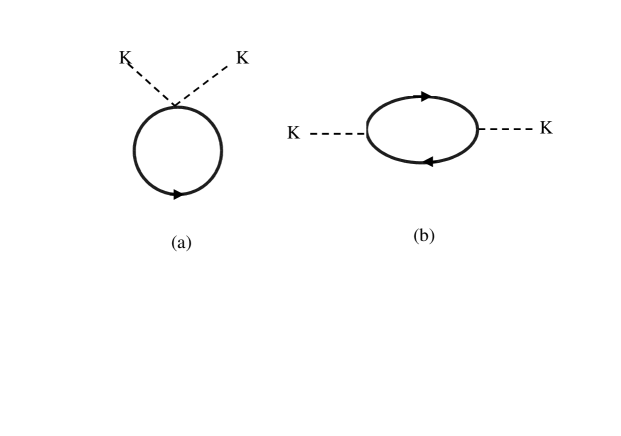
Figure 14: In-medium one-loop graphs contributing to energy-density of dense nuclear matter proportional to $v_{K}^{2}$ for kaon condensation. The solid line stands for baryons and the dotted line for the kaon.

Within the one-loop approximation, the p-wave interaction is linear in the square of the kaon three-momentum. Thus for a density for which

$$\rho\left[\frac{(3F+D)^{2}}{8(d-2b)m_{s}f^{2}}+\frac{(D-F)^{2}}{8dm_{s}f^{2}}\right]>1$$ (III.176)

which corresponds to the density $\rho>\sim 3.2\rho_{0}$, increasing $\vec{q}^{2}$ would bring in increasing attraction triggering a $K^{0}$ condensation. However in reality, there is a form factor associated with the vertex (which in the chiral counting would correspond to higher loops) that would prevent the arbitrary increase in the momentum. It is likely that the LHS of (III.176) is never greater than 1 in which case one would have $\vec{q}^{2}=0$. Let us assume this for the moment and ignore the $K^{0}$ mode. We now minimize the energy density $\epsilon$ with respect to the pion momentum and $K^{-}$ momentum. From $\partial\tilde{\epsilon}/\partial\vec{p}_{\pi}=0$, we get

$$\mu=(F+D)^{2}\frac{\rho}{2f^{2}}.$$ (III.177)

We will confine to s-wave KN interactions and set $\vec{k}=0$. Then the charge neutrality $\partial\tilde{\epsilon}/\partial\mu=0$ gives

$$\vec{p}_{\pi}^{2}=\left(\frac{\rho}{2f^{2}}\right)^{2}(F+D)^{2}\left\{[2(F+D)^{2}-1]+[2(F+D)^{2}+1]|\frac{v_{K}}{v_{\pi}}|^{2}\right\}.$$ (III.178)

We thus have

$$\tilde{\epsilon} = \epsilon(v_{\pi},v_{K})=\epsilon(0,0)$$ (III.179)

$$+ |v_{\pi}|^{2}\left\{m_{\pi}^{2}-(F+D)^{2}\left(\frac{\rho}{2f^{2}}\right)^{2}[(F+D)^{2}-1]\right\}$$

$$+ |v_{K}|^{2}\left\{m_{K}^{2}-(F+D)^{2}\left(\frac{\rho}{2f^{2}}\right)^{2}[(F+D)^{2}+1]+\left(\frac{\rho}{2f^{2}}\right)(4h+2d)m_{s}\right\}$$

$$+ \cdots.$$

What is known from an extensive theoretical and experimental development in nuclear physics, particularly from nuclear beta decay and spin-isospin modes in complex nuclei is that the main correlation effect which would correspond to higher order chiral corrections in the framework of chiral perturbation expansion is the downward renormalization of the axial-vector coupling constant $g_{A}$ from its free space value of $1.26$ to about $1$ discussed in the previous subsection. This means that the main correction to the above formula would be to replace $(F+D)$ above by $g_{A}^{*}\approx 1$. Including nucleon-nucleon interaction effects generated through the contact interaction of (III.88) in the particle-hole spin-isospin channel will further reduce the effective $g_{A}$, as is well-known in the Landau-Migdal formalism. This makes the coefficient of $|v_{\pi}|^{2}$ always greater than zero to a much larger density than relevant here. Therefore we expect that

$$v_{\pi}\approx 0.$$ (III.180)

The vanishing VEV of the pion field in the presence of a nonvanishing kaon VEV would imply by (III.178) an arbitrarily large pion momentum. Such a situation would be prevented by form factor effects arising at higher loop order. Since there cannot be any kaon condensation without pions (condensed or not) (this can be easily verified by looking at the energy density in the absence of pion field and showing that the coefficient of $|v_{K}|^{2}$ is always greater than zero), it pays to have a little bit of pion VEV at the cost of a large pion momentum. What matters is that the pion contribution to the energy density be as small as possible, not necessarily strictly zero.

The critical density for kaon condensation $\rho_{K}$ is

$$\rho_{K}\approx-f^{2}m_{s}(2h+d)\left\{[1+\frac{2m_{K}^{2}}{m_{s}^{2}(2h+d)^{2}}]^{\frac{1}{2}}-1\right\}$$ (III.181)

where we have set $g_{A}^{*}\approx 1$. Numerically this gives $\rho_{K}\approx 2.6\rho_{0}$ for $hm_{s}=-310$ MeV and $\rho_{K}\approx 3.7\rho_{0}$ for $hm_{s}=-140$ MeV (which is close to $hm_{s}=-125$ MeV corresponding to the extreme case with $m_{s}\langle p|\bar{s}s|p\rangle\approx 0$). Even when $(g_{A}^{*})^{2}=1/2$, the critical density increases only to about 5.7 times $\rho_{0}$. This is of course too high a density for the approximations used to be valid. Nonetheless one observes here a remarkable robustness against changes in parameters, in particular with respect to the greatest uncertainty in the theory, namely the quantity $h$ and also $g_{A}^{*}$. The insensitivity to the strangeness content of the proton, namely, the parameter $(h+d)$ makes the prediction surprisingly solid. Furthermore, while $(F+D)\rightarrow 1$ banishes the pion condensation, this affects relatively unimportantly the kaon property. It seems significant that the critical density for kaon condensation is robust against higher-order corrections while pion condensation is extremely sensitive to higher-order graphs.

Unfortunately it is highly unlikely that Nature provides the right condition for pions to trigger this mode of kaon condensation. The trouble is that once $g_{A}^{*}$ falls to near 1 or below, the condensate pion momentum has to be large and this would be prevented by the form factors that one would have to append to pion-nucleon vertices. Furthermore if the kaon condensation occurs at large density, say, at five or six times the matter density, then many of the approximations used so far (such as the heavy-baryon approximation) would no longer be justifiable.

4.2.2 Kaon condensation via electron chemical potential

In the above discussion, pions played a crucial role in triggering kaon condensation. Here we present an alternative way for the kaons to condense in “neutron star” matter which does not require pion condensation. The key idea is that in “neutron star” matter, energetic electrons – reaching hundreds of MeV in kinetic energy in dense “neutron star” matter – can decay into kaons if the kaon mass falls sufficiently low in dense matter, as we will show below [128], via

$$e^{-}\rightarrow K^{-}+\nu.$$ (III.182)

This process can go into chemical equilibrium with the beta decay

$$n\rightarrow p+e^{-}+\nu_{e}$$ (III.183)

with the neutrinos diffusing out. This means that the chemical potentials satisfy

$$\mu_{K^{-}}=\mu_{e^{-}}=\mu_{n}-\mu_{p}\ .$$ (III.184)

Let $x$ denote the fraction of protons generated by (III.182) and (III.183), so

$$\rho_{n}=(1-x)\rho,\ \ \ \ \rho_{p}=x\rho$$ (III.185)

and define

$$\rho\equiv u\rho_{0}$$ (III.186)

with $\rho_{0}$ being the nuclear matter density. With the addition of protons, we gain in energy (i.e, the symmetry energy) by the amount

$$E_{s}/V=\epsilon_{s}[(1-2x)^{2}-1]\rho_{0}u=-4x(1-x)\epsilon_{s}\rho_{0}u$$ (III.187)

where we have assumed, for simplicity, that the symmetry energy depends on the density linearly with the constant $\epsilon_{s}$ determined from nuclei,

$$\epsilon_{s}\approx 32{\rm MeV}.$$ (III.188)

More sophisticated formulas for symmetry energy could be used but for our purpose this form should suffice. In any event the symmetry energy above nuclear matter density is unknown, so this constitutes one of the major uncertainties in our discussion.

Instead of (III.174), we have a simpler form for the energy density,

$$\tilde{E}/V\equiv\tilde{\epsilon} = \tilde{\epsilon}(0)+(m_{K}^{2}-\mu^{2})|v_{K}|^{2}+\rho\Delta\epsilon$$ (III.189)

where $\tilde{\epsilon}(0)$ represents the sum of the kinetic energy density of the symmetric nuclear matter and the isospin independent part of the nuclear interaction contribution and

$$\Delta\epsilon=-\frac{1}{2f^{2}}\left[\mu(1-x)+2\mu x-(4h+2d)m_{s}\right]|v_{K}|^{2}-4x(1-x)\epsilon_{s}+\cdots$$ (III.190)

The first term in the square bracket of (III.190) is the neutron contribution through vector exchange (namely, the $V_{0}$ term in (III.158)) and the second the corresponding proton contribution. The factor of 2 for the proton contribution can be easily understood by the fact that the $K^{-}p$ interaction with vector meson exchanges is twice as attractive as the $K^{-}n$ interaction: This can be readily verified by looking at the isospin structure of the vector current $V_{\mu}$. Defining

$$\hat{\mu}=\mu+\frac{\rho_{0}u}{4f^{2}}(1+x)$$ (III.191)

we can rewrite (III.189)

$$\Delta\epsilon \equiv \tilde{\epsilon}-\tilde{\epsilon}(0)$$ (III.192)

$$= \left[(m_{K}^{*})^{2}-\hat{\mu}^{2}+\frac{\rho_{0}^{2}u^{2}}{16f^{4}}(1+x)^{2}\right]|v_{K}|^{2}-4x(1-x)\epsilon_{s}\rho_{0}u+x\rho_{0}u\mu$$

where

$$(m_{K}^{*})^{2}=m_{K}^{2}+\frac{\rho_{0}u}{2f^{2}}(4h+2d)m_{s}.$$ (III.193)

The charge neutrality condition is gotten by balancing the negative charge of the kaon against the positive charge of the proton, i.e,

$$\hat{\mu}=x\frac{\rho_{0}u}{2|v_{K}|^{2}}.$$ (III.194)

The condition (III.194) gives $x$ as a function of $|v_{K}|^{2}$ since the proton and neutron chemical potentials are functions of $x$. Since by beta equilibrium,

$$\partial\tilde{\epsilon}/\partial x=0,$$ (III.195)

we have one more condition

$$\hat{\mu}\approx\frac{\rho u}{2f^{2}}(1+x)=\frac{16f^{2}}{|v_{k}|^{2}}x(1-2x)\epsilon_{s}.$$ (III.196)

Substituting (III.194) and (III.196) into (III.192) with the electron contribution taken into account and using the numerical values $dm_{s}\approx 134$ MeV, $hm_{s}\approx-310$ MeV (consistent with lattice results discussed in Chapter 9), $\epsilon_{s}\approx 32$ MeV, $f=93$ MeV, we find the critical density

$$\rho_{K}\approx 2\rho_{0}.$$ (III.197)

This critical density is comparable to that predicted for the most optimistic case of the kaon condensation triggered by pion condensation. The more sophisticated calculation described later using the same physical mechanism and chiral perturbation theory corroborated this simple estimate.

An extremely interesting question to ask for physics of neutron stars and stellar collapse is what the proton fraction $x$ comes out to be in neutron star matter given the low critical density predicted for the kaon condensate formation. This is highly relevant for neutron star cooling. It is known that kaon condensation by itself could lead to a rapid cooling [129]. But even more importantly, as pointed out recently by Lattimer et al [130], the direct URCA process can occur in neutron stars if the proton concentration exceeds some critical value in the range of $(11-15)\%$: The direct URCA can cool the neutron star considerably faster than any other known mechanism, be that meson condensation or quark-gluon plasma. In order to evaluate the proton concentration, we have to include higher order (at least quartic) terms in kaon field. In free space, kaon-kaon interactions are are known to be weak, so we may ignore them. However medium-dependent kaon-kaon interactions, appearing at the one-loop level, may not be negligible. This requires calculating density-dependent loop diagrams. In the absence of explicit computation of the loop diagrams, it is difficult to say what the proton fraction comes out to be. Here we attempt a simple calculation of $x$ which may not be accurate but nevertheless gives some idea how things will go.

Even if one ignores the explicit loop graphs, our expression for the energy density contains an arbitrary power of the kaon VEV through the relation between $x$ and $|v_{K}|^{2}$, namely from eqs.(III.194) and(III.196),

$$x=(8\epsilon_{s}/\rho_{0})|v_{K}|^{2}\left(1+(16\epsilon_{s}/\rho_{0})|v_{K}|^{2}\right)^{-1}.$$ (III.198)

In looking for the critical density, it sufficed to retain only the lowest order term in the VEV from this relation. For determining the proton fraction $x$, however, we need higher orders, certainly at least quartic. It may be that it is not really justified to take into account the higher VEV’s through solely the nonlinearity of the charge neutrality constraint while ignoring explicit contributions from higher loop graphs but to the extent that we are using a “phenomenological” symmetry energy, it may be hoped that the constraint equation supplies not entirely erroneous higher-order VEV’s. Now it is easy to check that expanding (III.198) to the quartic order in the VEV is not good enough. The resulting quartic term in the energy density is much too repulsive for the kaon VEV to develop significantly. It is not surprising that the expansion cannot be trusted if truncated at low order since next order terms that are ignored have much larger coefficients with alternating sign. Instead of expanding it, therefore, we should substitute (III.198) into (III.192) and minimize the resulting energy density with respect to $|v_{K}|^{2}$. The resulting algebraic equation has been solved exactly for the VEV as a function of $u$. The result (obtained without the scaling effect) is that the critical proton concentration $x_{c}=0.11$ is reached at the density $u=4$, increasing gently as density increases, i.e, $x=0.12$ at $u=5$, $x=0.17$ at $u=10$ etc. The scaling effect as well as any further attraction (expected) from loop contributions will increase further the proton concentration. It looks that the URCA process is very likely to play an important role.

4.2.3 Constraints from kaon-nuclear interactions

Although the effective chiral Lagrangian is consistent with nuclear matter when scale anomaly is suitably incorporated, we have not asked whether it is consistent with on-shell kaon interactions with nucleons, both in free space and in medium. To answer this question, we extract relevant terms for s-wave kaon-nucleon scattering from the Lagrangian density (III.158). The leading term is of order $Q^{1}$ or $\nu=1$ and has the form

$${\cal L}_{\nu=1}(KN)=\frac{-i}{8f_{\pi}^{2}}\left(3({\overline{N}}\gamma^{0}N)\bar{K}\leftrightarrow K+({\overline{N}}\vec{\tau}\gamma^{0}N)\cdot\bar{K}\vec{\tau}\leftrightarrow K\right)$$ (III.199)

with $N^{T}=(p\ \ n)$, $K^{T}=(K^{+}\ K^{0})$ and ${\overline{K}}\leftrightarrow K\equiv{\overline{K}}\rightarrow K-{\overline{K}}\leftarrow K$. For $\bar{K}N$ scattering (with $\bar{K}^{T}=(K^{-}\ \bar{K}^{0})$), due to G-parity, the isoscalar term changes sign. In terms of an effective Lagrangian that contains vector mesons in hidden gauge symmetric way, the first term of (III.199) cam be identified as the $\omega$ exchange and the second term as the $\rho$ exchange between the kaon and the nucleon. Thus this leading order term can be thought of as vector-dominated for the scattering amplitude. Now the next order term is of $\nu=2$ and can be written for s-wave scattering as

$${\cal L}_{\nu=2}(KN) = \frac{\Sigma_{KN}}{f_{\pi}^{2}}({\overline{N}}N){\overline{K}}K+\frac{C}{f_{\pi}^{2}}(\bar{N}\vec{\tau}N)\cdot(\bar{K}\vec{\tau}K)$$ (III.200)

where

$$\Sigma_{KN} = -(\frac{1}{2}b+d+2h)m_{s},$$ (III.201)

$$C = -\frac{bm_{s}}{2},$$ (III.202)

With (III.199) and (III.200), the s-wave $KN$ scattering lengths are

$$a_{I=1}^{KN} = \frac{1}{4\pi f_{\pi}^{2}(1+m_{K}/m_{B})}\left(-m_{K}+\Sigma_{KN}+C\right),$$ (III.203)

$$a_{I=0}^{KN} = \frac{1}{4\pi f_{\pi}^{2}(1+m_{K}/m_{B})}\left(\Sigma_{KN}-3C\right).$$ (III.204)

With the values for the constants $b$, $d$ and $h$ given above (III.164)- (III.166), that is, $bm_{s}=-67$ MeV, $dm_{s}=134$ MeV and $hm_{\approx}-310$ MeV (which imply $\Sigma_{KN}\approx 520$ MeV), we get $a_{I=1}^{KN}\approx 0.07$ fm and $a_{I=0}^{KN}\approx 0.50$ fm to be compared with the presently available empirical values $-0.31$ fm and $-0.09$ fm respectively. The empirical value for $a_{I=1}^{KN}$ is reliable but that for $a_{I=0}^{KN}$ is not. In fact the latter is compatible with zero fm. The experimental uncertainty notwithstanding, it is clear that the Lagrangian so far used is not consistent with the s-wave $K^{+}N$ scattering. It is true that the $\Sigma_{KN}$ that large implies a substantial amount of strangeness in the proton which is not in accord with Nature. If one lowers the value of $\Sigma_{KN}$ to $\sim 2m_{\pi}$ which is reasonable for the strangeness content, the predicted values are: $a_{I=1}^{KN}\approx 0.07$ fm and $a_{I=0}^{KN}\approx 0.50$ fm. These are closer to the empirical values but the $I=0$ amplitude is much too attractive. The point is that if the amplitudes for the $K^{+}N$ channel come out wrong, there is no way that the amplitudes for the $K^{-}N$ channel can come out right: The $K^{-}N$ interaction is much stronger than the $K^{+}N$ interaction.

This difficulty can be remedied if one recognizes that the $\nu=2$ piece of the Lagrangian (III.200) is incomplete. It misses the chiral symmetric two-derivative terms which for s-wave scattering take the form

$$\delta{\cal L}_{\nu=2}(KN)=\frac{\tilde{D}}{f_{\pi}^{2}}({\overline{N}}N)\partial_{t}{\overline{K}}\partial_{t}K+\frac{\tilde{D}^{\prime}}{f_{\pi}^{2}}({\overline{N}}\vec{\tau}N)\cdot(\partial_{t}{\overline{K}}\vec{\tau}\partial_{t}K).$$ (III.205)

There are two sources to these terms. One is what we will call “$1/m$” correction. This comes because in the heavy-baryon formalism, baryon-antibaryon pair terms appear at the $\nu=2$ order in the form of $p/m_{N}$ where $p$ is the spatial momentum carried by the nucleon. The other source has to do with high-energy degrees of freedom integrated out above the chiral scale $\Lambda_{\chi}$, appearing as contact counter terms. The former can be calculated but the latter, while calculable in some dynamical models, are unknown constants that need be fixed by experiments. Including (III.205) modifies the scattering lengths to

$$a_{I=1}^{KN} = \frac{1}{4\pi f_{\pi}^{2}(1+m_{K}/m_{B})}\left(-m_{K}+\Sigma_{KN}+C+(\bar{D}+\bar{D}^{\prime}))m_{K}^{2}\right),$$ (III.206)

$$a_{I=0}^{KN} = \frac{1}{4\pi f_{\pi}^{2}(1+m_{K}/m_{B})}\left(\Sigma_{KN}-3C+(\bar{D}-3\bar{D}^{\prime})m_{K}^{2}\right).$$ (III.207)

Let us first ask what values of $\tilde{D}$ and $\tilde{D}^{\prime}$ are needed for (III.206) and (III.207) to reproduce the experimental numbers. We find:

$$\tilde{D} \approx 0.33/m_{K}-\Sigma_{KN}/m_{K}^{2},$$ (III.208)

$$\tilde{D}^{\prime} \approx 0.16/m_{K}-C/m_{K}^{2}.$$ (III.209)

For $\tilde{D}$, we take $\Sigma_{KN}\approx 2m_{\pi}$. We have $\tilde{D}\approx-0.24/m_{K}$ and $\tilde{D}^{\prime}\approx 0.23/m_{K}$.

As mentioned, the $1/m$ corrections are calculable. They are given by [131]

$$\tilde{D}_{\frac{1}{m}} \approx -\frac{1}{48}\left[(D+3F)^{2}+9(D-F)^{2}\right]/m_{N}\approx-0.06/m_{K},$$

$$\tilde{D}^{\prime}_{\frac{1}{m}} \approx -\frac{1}{48}\left[(D+3F)^{2}-3(D-F)^{2}\right]/m_{N}\approx-0.04/m_{K}.$$ (III.210)

Clearly the $1/m$ corrections are much too small to account for the values of $\tilde{D}$ and $\tilde{D}^{\prime}$. The main contributions must therefore come from the contact counter terms since at order $\nu=2$, there are no loop corrections which start at $\nu=3$.

Given that the $\tilde{D}$ and $\tilde{D}^{\prime}$ are very important at threshold, an immediate question is how they affect the critical density and composition of the condensed matter. Since these terms are quadratic in derivative, for the s-wave processes we are considering, they will simply modify $\omega^{2}$ coming from the kinetic energy term for the kaon as

$$\omega^{2}\rightarrow\left(1+[\frac{\tilde{D}}{f_{\pi}^{2}}+(2x-1)\frac{\tilde{D}^{\prime}}{f_{\pi}^{2}}]u\rho_{0}\right)\omega^{2}.$$ (III.211)

At threshold, $\omega\rightarrow m_{K}$. For kaon condensation, as mentioned above, $\omega=\mu$ ($\mu$ being the chemical potential) due to the charge conservation. Now since in dense matter the chemical potential gets quenched, the role of the $\tilde{D}$ and $\tilde{D}^{\prime}$ terms becomes less important. For this reason, little is modified in the properties of the condensate by the inclusion of these extra terms. For instance, with $\Sigma_{KN}\approx 2m_{\pi}$ and without the BR scaling, the critical density is $u_{c}\approx 3.04$ without $\tilde{D}$ and $\tilde{D}^{\prime}$ and $u_{c}\approx 3.27$ with them. The equation of state is also little affected, the matter turning rapidly to “nuclear matter” with both $x$ and strangeness fraction $S/B$ near 0.5 right above the critical point. This feature is expected to have a profound influence on the formation of compact “nuclear stars” and their cooling. We will not pursue this here but refer to the literature [131].

4.3 Vector Symmetry

What happens when density is so high that there is a phase transition away from the Goldstone mode? Does it go into quark-gluon phase as expected at some density by QCD? Or does it make a transition into something else? Up to date, this question has not received a clear answer: It remains an open question even after so many years of QCD. Here we discuss a possible state of matter that is still hadronic but different from the normal hadron state and also from meson-condensed states – a state that realizes the “vector symmetry” of Georgi[121]. 

4.3.1 Pseudoscalar and scalar Goldstone bosons

When one has the matrix element of the axial current

$$\langle 0|A^{\mu}|\pi\rangle=iq^{\mu}f_{\pi}$$ (III.212)

this can mean either of the two possibilities. The conventional way is to consider $\pi$’s as Goldstone bosons that emerge as a consequence of spontaneous breaking of chiral $SU(3)\times SU(3)$ symmetry, with the current $A^{\mu}$ associated with the part of the symmetry that is broken (i.e, the charge $\int d^{3}xA_{0}(x)$ being the generator of the broken symmetry). But there is another way that this relation can hold. If there are scalar bosons $s$ annihilated by the vector current $V^{\mu}$

$$\langle 0|V^{\mu}|s\rangle=iq^{\mu}f_{s}$$ (III.213)

with $f_{\pi}=f_{s}$, then the symmetry $SU(3)\times SU(3)$ can be unbroken. This can happen in the following way. Since $A^{\mu}$ and $V^{\mu}$ are part of $(8,1)+(1,8)$ of $SU(3)\times SU(3)$, all we need is that $\pi$’s and $s$’s are part of $(8,1)+(1,8)$. The $SU(3)\times SU(3)$ symmetry follows if the decay constants are equal. In Nature, one does not see low-energy scalar octets corresponding to $s$. Therefore the symmetry must be broken. This can be simply understood if one imagines that the scalars are eaten up to make up the longitudinal components of the massive octet vector mesons. If this is so, then there must be a situation where the symmetry is restored in such a way that the scalars are liberated and become real particles, with the vectors becoming massless. This is the “vector limit” of Georgi. In this limit, there will be 16 massless scalars and massless octet vector mesons with the symmetry swollen to $[SU(3)]^{4}$ which is broken down spontaneously to $[SU(3)]^{2}$. In what follows, we discuss how this limit can be reached.

The full vector symmetry  is

$$SU_{L}(3)\times SU_{R}(3)\times SU_{G_{L}}(3)\times SU_{G_{R}}(3).$$ (III.214)

This is a primordial symmetry which is dynamically broken down to

$$SU_{L+G_{L}}(3)\times SU_{R+G_{R}}(3).$$ (III.215)

As is well-known, the nonlinear symmetry

$$\frac{SU_{L}(3)\times SU_{R}(3)\times SU_{G_{L}}(3)\times SU_{G_{R}}(3)}{SU_{L+G_{L}}(3)\times SU_{R+G_{R}}(3)}$$ (III.216)

is equivalent to the linear realization

$$\{[SU_{L}(3)\times SU_{G_{L}}(3)]_{global}\times[SU_{L}(3)]_{local}\}\times\{L\rightarrow R\}$$ (III.217)

where the local symmetries are two copies of the hidden gauge symmetry. One can think of the two sets of hidden gauge bosons as the octet vectors $\rho_{\mu}$ and the octet axial vectors $a_{\mu}$.

In order to supply the longitudinal components of both vector and axial vector octets of spin-1 fields, we would need 16 Goldstone bosons that are to be eaten up plus 8 pseudoscalars $\pi$ to appear as physical states. Here we shall consider a minimal model where only the vector fields $\rho$ are considered. The axials are purged from the picture. We can imagine this happening as an explicit symmetry breaking

$$SU_{G_{L}}\times SU_{G_{R}}\rightarrow SU_{G_{L}+G_{R}}.$$ (III.218)

What happens to the axials after symmetry breaking is many-fold. They could for instance be banished to high mass $\gg m_{\rho}$.

4.3.2 The Lagrangian

To be more specific, we shall construct a model Lagrangian with the given symmetry. Since we are ignoring the axials, the Goldstone bosons can be represented with the transformation properties

$$\xi_{L} \rightarrow L\xi_{L}G^{\dagger},$$ (III.219)

$$\xi_{R} \rightarrow R\xi_{R}G^{\dagger}$$ (III.220)

with $\xi_{L}$ transforming as $(3,1,\bar{3})$ under $SU_{L}(3)\times SU_{R}(3)\times SU_{G}(3)$ (with $G=G_{L}+G_{R}$) and $\xi_{R}$ as $(1,3,\bar{3})$. $L$, $R$ and $G$ are the linear transformations of the respective symmetries. The usual Goldstone bosons of the coset $SU_{L}(3)\times SU_{R}(3)/SU_{L+R}(3)$ are

$$U=\xi_{L}\xi_{R}^{\dagger}$$ (III.221)

transforming as $(3,\bar{3},1)$. In terms of the covariant derivatives

$$D^{\mu}\xi_{L} = \partial^{\mu}\xi_{L}-ig\xi_{L}\rho^{\mu},$$ (III.222)

$$D^{\mu}\xi_{R} = \partial^{\mu}\xi_{R}-ig\xi_{R}\rho^{\mu}$$ (III.223)

the lowest derivative Lagrangian having the (hidden) local $SU(3)_{L+R}$ symmetry is

$${\cal L}=\frac{f^{2}}{2}\{{\mbox{Tr}}\left(D^{\mu}\xi_{L}D_{\mu}\xi_{L}^{\dagger}\right)+(L\rightarrow R)\}+\kappa\frac{f^{2}}{4}{\mbox{Tr}}(\partial^{\mu}U\partial_{\mu}U^{\dagger}).$$ (III.224)

A convenient parameterization for the chiral field is

$$\xi_{\mbox{\tiny{L,R}}}\equiv e^{i\sigma(x)/f_{s}}e^{\pm i\pi(x)/f_{\pi}}$$ (III.225)

with $\sigma(x)=\frac{1}{2}\lambda^{a}\sigma^{a}(x)$ and $\pi(x)=\frac{1}{2}\lambda^{a}\pi^{a}(x)$. (Setting $\sigma(x)=0$ corresponds to unitary gauge with no Faddeev-Popov ghosts.) At the tree order with the Lagrangian (III.224), we have

$$f_{s}=f,\ \ \ \ \ f_{\pi}=\sqrt{1+\kappa}f$$ (III.226)

and the $\rho\pi\pi$ coupling

$$g_{\rho\pi\pi}=\frac{1}{2(1+\kappa)}g.$$ (III.227)

The vector meson mass is

$$m_{\rho}=fg=2\sqrt{1+\kappa}f_{\pi}g_{\rho\pi\pi}.$$ (III.228)

Thus $f_{s}=f_{\pi}$ when $\kappa=0$, i.e, when the mixing $LR$ vanishes. One can see that the standard hidden gauge symmetry result is obtained when $\kappa=-1/2$. When $\kappa=0$, we have an unbroken $SU(3)\times SU(3)$, but the vectors are still massive. The mass can disappear even if $f_{\pi}\neq 0$ if the gauge coupling vanishes. In the limit that $g\rightarrow 0$ which is presumably attained at asymptotic density as described below, the vector mesons decouple from the Goldstone bosons, the scalars are liberated and the symmetry swells to $[SU(3)]^{4}$ with the Goldstone bosons transforming

$$\xi_{L} \rightarrow L\xi_{L}G_{L}^{\dagger},$$ (III.229)

$$\xi_{R} \rightarrow R\xi_{R}G_{R}^{\dagger}.$$ (III.230)

Note that the local symmetry $G$ gets “recovered” to a global symmetry $G_{L}\times G_{R}$. (This is a dynamical symmetry restoration, in some sense.)

4.3.3 Hidden gauge symmetry and the vector limit

We shall now consider renormalization-group (RG) structure  of the constants $g$ and $\kappa$ of the Lagrangian in $SU(2)$ flavor which is of the form (III.224) with the fields valued in $SU(2)$,

$${\cal L}=\frac{f^{2}}{2}\{{\mbox{Tr}}\left(D^{\mu}\xi_{L}D_{\mu}\xi_{L}^{\dagger}\right)+(L\rightarrow R)\}+\kappa\frac{f^{2}}{4}{\mbox{Tr}}(\partial^{\mu}U\partial_{\mu}U^{\dagger}).$$ (III.231)

The kinetic energy term of the $\rho$ field should be added for completeness; we do not need it for this discussion. We are interested in what happens to hadrons described by this Lagrangian as matter density $\rho$ and/or temperature $T$ are increased . For this consider the vector meson mass in dense medium at zero temperature. It turns out that the mass formula (III.228) is valid to all orders of perturbation theory [132, 133]. We expect this to be true in medium, according to the argument given above. Therefore we need to consider the scaling behavior of the constants $f_{\pi}$, $g$ and $\kappa$ in medium. Now we know from above that $f_{\pi}$ decreases as density is increased. This is mainly caused by the vacuum property, so we can assume that the effect of radiative corrections we are considering is not important. Thus we have to examine how $g$ and $\kappa$ scale. The quantities we are interested in are the $\beta$ functions for the coupling constants $g$ and $\kappa$. These can be derived in a standard way with the Lagrangian (III.231). At one-loop order, we have in dimensional regularization [132]

$$\beta_{g}(g_{r}) \equiv \mu\frac{dg_{r}}{d\mu}=-\frac{87-a_{r}^{2}}{12}\frac{g_{r}^{3}}{(4\pi)^{2}},$$ (III.232)

$$\beta_{a}(a_{r}) \equiv \mu\frac{da_{r}}{d\mu}=3a_{r}(a_{r}^{2}-1)\frac{g_{r}^{2}}{(4\pi)^{2}}$$ (III.233)

where $\mu$ is the length scale involved (which in our case is the matter density) and we have redefined

$$a=1/(1+\kappa).$$ (III.234)

To see how the factors in the beta function can be understood, let us discuss the first equation describing the way the coupling constant $g$ runs. In terms of Feynman diagrams, the quantity on the right-hand side of (III.232) can be decomposed as

$$-\frac{1}{(4\pi)^{2}}\frac{87-a_{r}^{2}}{12}=-\frac{1}{(4\pi)^{2}}\left[\frac{11n_{f}}{3}-(\frac{1}{2})^{2}\frac{1}{3}-(\frac{a_{r}}{2})^{2}\frac{1}{3}\right]$$ (III.235)

with the number of flavor $n_{f}=2$. This is an exact analog to the beta function of QCD, $\beta_{g}^{\mbox{\tiny QCD}}=-\frac{g^{3}}{(4\pi)^{2}}\left[\frac{11}{3}N_{c}-\frac{2}{3}n_{f}\right]$. The first term on the right-hand side of (III.235) is the vector meson loop which is an analog to the gluon contribution in QCD with the number of flavors $n_{f}$ replacing the number of colors $N_{c}$ (the vector meson $\rho$ is the “gauge field” here), the second term is the $\sigma$ loop contribution $g_{\rho\sigma\sigma}^{2}/3$ with $g_{\rho\sigma\sigma}=g/2$ and the last term the pion loop contribution $g_{\rho\pi\pi}^{2}/3$ with $g_{\rho\pi\pi}=(a_{r}/2)g$.

As in QCD, the fact that the beta function is negative signals that the coupling constant runs down as the momentum (or density) scale increases and at asymptotic momentum (or density), the coupling would go to zero, that is, asymptotically free. Now the beta function is negative here as long as $a_{r}^{2}<87$ with the coupling constant running as

$$g^{2}(\mu)=\frac{8\pi^{2}}{(87-a_{r}^{2})\ln\frac{\mu}{\Lambda}}$$ (III.236)

with the HGS scale $\Lambda$ defined as in QCD. The inequality $a_{r}^{2}<87$ is clearly satisfied as one can see from Eq. (III.233) which says that there is an ultraviolet fixed point $a_{r}=1$, so as the momentum increases the constant $a$ would run toward 1. Of course one would have to solve the equations (III.232) and (III.233) simultaneously to see the trajectory of $a_{r}$ but it seems reasonable to assume that the $a_{r}$ runs monotonically from the vacuum value $a_{r}=2$ (or $\kappa=1$) to the fixed point $a_{r}=1$ (or $\kappa=0$). The in-medium mass formula

$$m_{\rho}^{\star}=f^{\star}g^{\star}=\frac{1}{\sqrt{1+\kappa^{\star}}}f_{\pi}^{\star}g^{\star}_{\rho\pi\pi}$$ (III.237)

shows that apart from the condensate effect on $f_{\pi}^{\star}$, there are additional effects due to the decreasing $(1+\kappa^{\star})^{-1}$ factor. The vector mass will go to zero for $f_{\pi}^{\star}\neq 0$ as the coupling $g^{\star}$ vanishes, approaching the “vector limit” of Georgi.

4.3.4 Physics under extreme conditions

What happens to the hadronic matter governed by the HGS Lagrangian as density or temperature increases? At present, there is no direct prediction from QCD that the relevant limits can be reached by temperature or density. No model calculations purporting to indicate them are available. Nonetheless, the vector limit ideas are intuitively appealing and could play an important role in dense cold matter like in nuclear stars and in hot dense matter like in heavy-ion collision.

In the $\kappa=0$ limit, the vector mass is

$$m_{\rho}=2f_{\pi}g_{\rho\pi\pi}$$ (III.238)

which in terms of physical values of $f_{\pi}$ and $g_{\rho\pi\pi}$ is too big by roughly a factor of $\sqrt{2}$ whereas the current algebra result (KSRF) is $m_{\rho}=\sqrt{2}f_{\pi}g_{\rho\pi\pi}$, which is in good agreement with the experiment. This shows that at the tree order, the limit is rather far from reality as applied to the medium-free space. Loop corrections with the Lagrangian treating the $\kappa$ term as a perturbation does improve the prediction[134], bringing it much closer to experiments. One possible scenario that emerges from the discussion given above is that the density changes the state of matter from the phase of normal matter with $\kappa\neq 0$ and $g\neq 0$ to first $\kappa=0$ and then to $g=0$, resulting in a significant increase of light degrees of freedom below the critical point. In the model we have been considering, we will have a total of 32 degrees of freedom consisting of 16 spin-0 bosons and 8 massless vectors. If we add the axial vectors, then the total becomes 48. Now in the quark-gluon phase with three flavors, one expects 47$\frac{1}{2}$. They are of the same order and if anything, the transition will be extremely smooth.

Strictly speaking, the above counting is not quite relevant because of the strange quark mass. The relevant degrees of freedom are more likely to be less than that. Nonetheless if one counts all the possible light degrees of freedom in the hadronic sector, they come out certainly much more than the customary counting based on pion degrees of freedom often invoked in the literature. Thus the vector limit is a possible candidate phase before the would-be chiral transition to quark-gluon phase (to be described in QCD variables) at which we will have $f_{\pi}=f_{s}=0$.

4.4 Appendix Added: Hidden Local Symmetry and Vector Manifestation of Chiral Symmetry

The idea that the Georgi vector limit is relevant to the chiral phase transition discussed in my ELAF93 lectures (given above) turns out to be only partially correct and the correct description comes from the major developments by Harada and Yamawaki on the “vector manifestation (VM)” of chiral symmetry [159, 160, 161, 162] reviewed recently in [163]. Indeed, at the phase transition, the gauge coupling $g$ vanishes, $g\rightarrow 0$, and $a\rightarrow 1$ as in the Georgi vector limit but contrary to Georgi’s case, the pion decay constant also has to go to zero. It turns out that this is a fixed point called “VM fixed point.” In this appendix, I describe briefly the essential points relevant to the phase transition phenomenon along the line that was presented in my 2002 Taiwan lecture note [146].

4.4.1 HLS and chiral perturbation theory

For completeness, I write down the full leading order (${{\cal O}}(p^{2})$) HLS Lagrangian explicitly:

$${\cal L}_{HLS}=F^{2}_{\pi}{\mbox{Tr}}(\hat{\alpha}_{A\mu})^{2}+F^{2}_{\sigma}{\mbox{Tr}}(\hat{\alpha}_{V\mu})^{2}-\frac{1}{2g^{2}}{\mbox{Tr}}(V_{\mu\nu})^{2}+{\cal L}_{p^{4}}.$$ (III.239)

with

$$\frac{F^{2}_{\sigma}}{F^{2}_{\pi}}=a$$ (III.240)

and

$$V_{\mu\nu} = \partial_{\mu}V_{\nu}-\partial_{\nu}V_{\mu}-i[V_{\mu},V_{\nu}],$$

$$\hat{\alpha}_{V\mu}(x) \equiv ({\cal D}_{\mu}\xi_{L}\cdot\xi_{L}^{\dagger}+{\cal D}_{\mu}\xi_{R}\cdot\xi_{R}^{\dagger})(-i/2),$$

$$\hat{\alpha}_{A\mu}(x) \equiv ({\cal D}_{\mu}\xi_{L}\cdot\xi_{L}^{\dagger}-{\cal D}_{\mu}\xi_{R}\cdot\xi_{R}^{\dagger})(-i/2)$$ (III.241)

and

$${\cal D}_{\mu}\xi_{L} = \partial_{\mu}-iV_{\mu}\xi_{L}+i\xi_{L}{\cal L}_{\mu},$$

$${\cal D}_{\mu}\xi_{R} = \partial_{\mu}-iV_{\mu}\xi_{R}+i\xi_{R}{\cal R}_{\mu}$$ (III.242)

where ${\cal L}_{\mu}$ and ${\cal R}_{\mu}$ are respectively left and right external gauge fields. I put the external gauge fields here since I will need them in considering correlators later. I have not put the mass term in (III.239) but it should be added for practical calculations. For the calculations to be described below, we need the Lagrangian of ${{\cal O}}(p^{4})$. If one includes the external gauge fields, there are some 35 terms in ${\cal L}_{p^{4}}$, the complete list of which can be found in the Phys. Rep. review of Harada and Yamawaki [163]. We won’t write it here in full. What we will need for our purpose are the ones that enter in the vector and axial-vector correlators and will be written down as needed.

As is done in chiral perturbation theory with the standard chiral Lagrangian without the vector mesons, we count

$$\partial_{\mu}\sim{\cal L}_{\mu}\sim{\cal R}_{\mu}\sim{{\cal O}}(p).$$ (III.243)

Here and in what follows, $p$ represents the characteristic small probe momentum involved. In the same counting the pion mass term will be $m_{\pi}^{2}\sim{\cal O}(p^{2})$ as the leading term in (III.239). It is in dealing with the vector mesons that one encounters an unconventional counting. As pointed out first by Georgi [121], in order to have a systematic chiral expansion with (III.239), the vector meson mass has to be counted as

$$m^{2}_{\rho}\sim m_{\pi}^{2}\sim{{\cal O}}(p^{2}).$$ (III.244)

Since $m^{2}_{\rho}\sim g^{2}f_{\pi}^{2}$, this means that we have to count $g\sim{{\cal O}}(p)$. Thus we should have

$$V_{\mu}\sim g\rho_{\mu}\sim{{\cal O}}(p).$$ (III.245)

This is how the vector kinetic energy term in (III.239) is of ${{\cal O}}(p^{2})$.

It might surprise some readers to learn that the vector meson mass has to be considered as “light” when in reality it is more than five times heavier than the pion mass in the vacuum. Even though one might argue that the expansion is $m_{\rho}^{2}/(4\pi F_{\pi})^{2}\sim 0.4$, this is not so small. Surprisingly enough, once one adopts this counting of the vector mass and the vector field, one can do a chiral perturbation calculation [160] that is equivalent to the classic calculation of Gasser and Leutwyler [101]. At this point it is important to note that while one may doubt the validity of the counting rule in the vacuum, it will however be fully justified in the scenario where the vector meson mass does become comparable to the pion mass as density approaches that of chiral restoration. So in some sense this counting rule which is valid at high density is being extrapolated down smoothly to the zero density regime.

If the Lagrangian (III.239) is to be taken as an effective field theory of QCD, then it can make sense only if the parameters of the Lagrangian are $bare$ parameters defined at a certain given scale. It is natural to define them at the chiral scale $\Lambda_{\chi}$ and that above $\Lambda_{\chi}$, it is QCD proper that is operative. Thus we are invited to match the HLS Lagrangian (III.239) to QCD at $\Lambda_{\chi}$ to determine the parameters. This matching will provide the $bare$ Lagrangian in the Wilsonian sense with which one can do quantum theory by “decimating” down to zero energy/momentum. The matching can be done typically with correlators in space-like momenta. We do this with the vector and axial-vector correlators defined as

$$i\int d^{4}xe^{iqx}\langle 0|TJ_{\mu}^{a}(x)J_{\nu}^{b}(0)|\rangle = \delta^{ab}\left(q_{\mu}q_{\nu}-g_{\mu\nu}q^{2}\right)\Pi_{V}(Q^{2}),$$

$$i\int d^{4}xe^{iqx}\langle 0|TJ_{5\mu}^{a}(x)J_{5\nu}^{b}(0)|\rangle = \delta^{ab}\left(q_{\mu}q_{\nu}-g_{\mu\nu}q^{2}\right)\Pi_{A}(Q^{2})$$ (III.246)

with

$$Q^{2}\equiv-q^{2}.$$ (III.247)

We first define the scale $\bar{\Lambda}$ at which the matching will be done. One would like to match the HLS theory and QCD at the point where both are “valid.” We suppose that the QCD correlators can be matched to those of HLS at $\bar{\Lambda}$ close to but slightly below $\Lambda_{\chi}$. At $\bar{\Lambda}$, the correlators in the HLS sector are supposed to be well described by tree contributions to ${\cal O}(p^{4})$ when $Q\sim\bar{\Lambda}$. To compute the tree graphs, we need the ${\cal O}(p^{4})$ Lagrangian that enters into the correlators,

$$\delta{\cal L}=z_{1}{\mbox{Tr}}\left[\hat{{\cal V}}_{\mu\nu}\hat{{\cal V}}^{\mu\nu}\right]+z_{2}{\mbox{Tr}}\left[\hat{{\cal A}}_{\mu\nu}\hat{{\cal A}}^{\mu\nu}\right]+z_{3}{\mbox{Tr}}\left[\hat{{\cal V}}_{\mu\nu}V^{\mu\nu}\right]$$ (III.248)

where $\hat{{\cal V}}_{\mu\nu}$ and $\hat{{\cal A}}_{\mu\nu}$ are respectively the external vector and axial-vector field tensors and $V_{\mu\nu}$ is the field tensor for the HLS vector defined above. The correlators in the HLS sector then are

$$\Pi^{(HLS)}_{A}(Q^{2}) = \frac{F_{\pi}^{2}(\bar{\Lambda})}{Q^{2}}-2z_{2}(\bar{\Lambda}),$$ (III.249)

$$\Pi^{(HLS)}_{V}(Q^{2}) = \frac{F_{\sigma}^{2}(\bar{\Lambda})}{M_{v}^{2}(\bar{\Lambda})+Q^{2}}\left[1-2g^{2}(\bar{\Lambda})z_{3}(\bar{\Lambda})\right]-2z_{1}(\bar{\Lambda})$$ (III.250)

with

$$M_{v}^{2}(\bar{\Lambda})\equiv g^{2}(\bar{\Lambda})F_{\sigma}^{2}(\bar{\Lambda}).$$ (III.251)

Since we are at the matching scale, there are no loops, i.e., no flow.

Next we have to write down the correlators in the QCD sector. We assume that these are given by the OPE to ${\cal O}(1/Q^{6})$,

$$\Pi^{(QCD)}_{A} = \frac{1}{8\pi^{2}}\left[-(1+\alpha_{s}/\pi)\ln\frac{Q^{2}}{\mu^{2}}+\frac{\pi^{2}}{3}\frac{\langle\frac{\alpha_{s}}{\pi}G_{\mu\nu}G^{\mu\nu}\rangle}{Q^{4}}+\frac{\pi^{3}}{3}\frac{1408}{27}\frac{\alpha_{s}\langle\bar{q}q\rangle^{2}}{Q^{6}}\right],$$ (III.252)

$$\Pi^{(QCD)}_{V} = \frac{1}{8\pi^{2}}\left[-(1+\alpha_{s}/\pi)\ln\frac{Q^{2}}{\mu^{2}}+\frac{\pi^{2}}{3}\frac{\langle\frac{\alpha_{s}}{\pi}G_{\mu\nu}G^{\mu\nu}\rangle}{Q^{4}}-\frac{\pi^{3}}{3}\frac{896}{27}\frac{\alpha_{s}\langle\bar{q}q\rangle^{2}}{Q^{6}}\right]$$ (III.253)

where $\mu$ here is the renormalization scale of QCD (e.g., in the sense of dimensional regularization) . Note that the QCD correlators separately depend explicitly on the renormalization scale $\mu$ but the difference does not. Such dependence must be lodged in the $z_{1,2}$ terms in the HLS sector. The condensates and the gauge coupling constant $\alpha_{s}$ of course depend implicitly on the scale $\mu$. In matching the QCD correlators to the HLS’ ones, the natural thing to do is to take $\mu\sim\bar{\Lambda}$.

The matching is done by equating the correlators and their derivatives at $Q^{2}=\bar{\Lambda}^{2}$. This gives effectively three equations. The parameters to be fixed are $F_{\pi}$, $g$, $a$, $z_{3}$ and $z_{2}-z_{1}$. That makes five parameters. To determine all five, the on-shell pion decay constant $F_{\pi}(0)=93$ MeV and the vector meson mass $m_{\rho}=770$ MeV are used as inputs. Given $\mu$, one can then fix all five constants at the scale $\bar{\Lambda}$. The HLS Lagrangian with the parameters so determined at $\bar{\Lambda}$ when implemented with RGE’s with certain quadratic divergences (to be described below) gives results that are very close to those obtained by the Gasser-Leutwyler Lagrangian [101] that includes ${\cal O}(p^{4})$ counter terms. This means that the counting rule used for the vector meson is consistent with chiral perturbation theory. Just to illustrate the point, let me give some numerical predictions given by the theory. With $\bar{\Lambda}=1.1\sim 1.2$ GeV, $\Lambda_{QCD}=400$ MeV, the results are:

$$g_{\rho} = 0.116\sim 0.118\ (0.118\pm 0.003),$$

$$g_{\rho\pi\pi} = 5.79\sim 5.95\ (6.04\pm 0.04),$$

$$L_{9}(m_{\rho}) = 7.55\sim 7.57\ (6.9\pm 0.7),$$

$$L_{10}(m_{\rho}) = -7.00\sim-6.23\ (-5.2\pm 0.3),$$

$$a(0) = 1.75\sim 1.85\ (2)$$ (III.254)

where the numbers in the parenthesis are experimental except for “a” which corresponds to VDM (or KSRF) value. For more details, see the Harada-Yamawaki review [163].

4.4.2 The “vector manifestation (VM)” fixed point

The HLS theory (III.239) has a set of fixed points when the scale is dialled. Among them there is only one fixed point called “vector manifestation (VM)” that matches with QCD. In the next subsection, I will show that that fixed point is relevant to chiral restoration when nuclear matter is compressed or heated.

We start with (III.239) defined at the scale $\bar{\Lambda}$, below which the relevant degrees of freedom are the pions $\pi$ and the vector mesons $\rho$ (and $\omega$). We would like to do the EFT as defined above by decimating downward from the scale $\bar{\Lambda}$. The parameters $F_{\pi}$, $g$, $F_{\sigma}$ (or $a$) and $z_{i}$ will flow as the renormalization scale ${\cal M}$ is dialled . To do this, one has to choose the gauge and the convenient gauge is the background gauge. These have been worked out in the background gauge [163] and to one-loop order, take the forms 

$${\cal M}\frac{dX}{d{\cal M}} = (2-3a^{2}G)X-2(2-a)X^{2},$$

$${\cal M}\frac{da}{d{\cal M}} = -(a-1)[3a(1+a)G-(3a-1)X],$$

$${\cal M}\frac{dG}{d{\cal M}} = -\frac{87-a^{2}}{6}G^{2},$$

$${\cal M}\frac{dz_{1}}{d{\cal M}} = C\frac{5-4a+a^{2}}{12},$$

$${\cal M}\frac{dz_{2}}{d{\cal M}} = C\frac{a}{6},$$

$${\cal M}\frac{dz_{3}}{d{\cal M}} = C\frac{1+2a-a^{2}}{6}$$ (III.255)

where

$$X({\cal M})\equiv C{\cal M}^{2}/F_{\pi}^{2}({\cal M}),\ \ G({\cal M})=Cg^{2},\ \ C=N_{f}/\left[2(4\pi)^{2}\right].$$ (III.256)

I should note that these are Wilsonian renormalization group equations valid above the vector meson mass scale $m_{\rho}$ defined by the on-shell condition $m_{\rho}^{2}=a(m_{\rho})g^{2}(m_{\rho})F_{\pi}^{2}(m_{\rho})$ at ${\cal M}=m_{\rho}$. This means that Equations (III.255) are valid for $a({\cal M})G({\cal M})\leq X({\cal M})$ but modified below by the decoupling of the vector mesons.

The fixed points are given by setting the RHS of (III.255) equal to zero. It is found in [162] that there are three fixed points in the relevant region with $a>0$ and $X>0$:

$$(X^{\star},a^{\star},G^{\star})=(1,1,0),(\frac{3}{5},\frac{1}{3},0),\left(\frac{2(2+45\sqrt{87})}{4097},\sqrt{87},\frac{2(11919-176\sqrt{87})}{1069317}\right)$$ (III.257)

and a fixed line

$$(X^{\star},a^{\star},G^{\star})=(0,{\rm any},0).$$ (III.258)

Depending upon how the parameters are dialled, there can be a variety of flows as the scales are varied. All the flows are interesting for the model per se. However not all of them are relevant to the physics given by QCD. In fact, if one insists that the vector and axial-vector correlators of HLS theory are matched at the chiral phase transition that is characterized by the on-shell pion decay constant $F_{\pi}({\cal M}=0)=0$ to those of QCD at a scale $\bar{\Lambda}\sim\Lambda_{\chi}$, then there is only one fixed point to which the theory flows and that is the vector manifestation (VM) fixed point

$$(X^{\star},a^{\star},G^{\star})_{VM}=(1,1,0).$$ (III.259)

This means that independently of what triggers the phase transition, at the chiral restoration point, the theory must be at the point $a=1,g=0,F_{\pi}=0$. As emphasized by Harada and Yamawaki, this is not Georgi’s “vector limit” [121] where $a=1,g=0$ but $F_{\pi}\neq 0$.

We will see next that density or temperature does indeed drive the system to the VM fixed point as does large $N_{f}$ and as a consequence, the vector meson mass must vanish at the chiral restoration point at least in the chiral limit. A corollary to this is that if an effective theory that has all the low-energy symmetries consistent with QCD but is not matched to QCD at an appropriate matching scale can flow in density/temperature in a direction that has nothing to do with QCD. In such a model, the vector meson mass need not vanish at the chiral transition point.

4.4.3 The fate of the vector meson in hot/dense matter

I will show that indeed, density or temperature can drive nuclear matter toward the VM fixed point and as a consequence, the vector meson mass must vanish at the critical point at least in the chiral limit. See [164]. Since the temperature case is quite similar to the density case, I will consider here only the density case. It is of course more relevant for studying the structure of compact-star matter. The same conclusion holds for high temperature case relevant to heavy-ion physics.

$\bullet$ Renormalization group equations for dense matterConsider a many-body hadronic system at a density $n$ or equivalently chemical potential $\mu$ ($n$ and $\mu$ will be used interchangeably). In the presence of matter density, the system loses Lorentz invariance and hence the theory should be formulated with an $O(3)$ invariance. This means that one has to separate the time and space components of vector objects (like currents etc.). It turns out that one can proceed as if we have Lorentz invariance and at the end of the day, make the distinction when necessary. The details of non-Lorentz invariant structure are given in the paper [164].

The Lagrangian density (III.239) including the ${\cal O}(p^{4})$ term contains no fermions and hence is not sufficient. To introduce fermion degrees of freedom, we assume that as one approaches the chiral transition point from below, the quasiquark (or constituent quark) description is more appropriate than baryonic. Denoting the quasiquark by $\psi$, we write the fermion part of the Lagrangian as

$$\delta{\cal L}_{F} = \bar{\psi}(x)(iD_{\mu}\gamma^{\mu}-\mu\gamma^{0}-m_{q})\psi(x)$$ (III.260)

$$+\bar{\psi}(x)\left(\kappa\gamma^{\mu}\hat{\alpha}_{\parallel\mu}(x)+\lambda\gamma_{5}\gamma^{\mu}\hat{\alpha}_{\perp\mu}(x)\right)\psi(x)$$

where $D_{\mu}\psi=(\partial_{\mu}-ig\rho_{\mu})\psi$ and $\kappa$ and $\lambda$ are constants to be specified later. The HLS Lagrangian we work with is then given by (III.239) and (III.260).

We consider matching at the scale $\bar{\Lambda}$. In the presence of matter, the matching scale will depend upon density. We use the same notation as in the vacuum with the $\mu$ dependence understood. At the scale $\bar{\Lambda}$, the correlators are given by the tree contributions and hence by (III.239) only. Since there is no flow, (III.260) which can figure only at loop order does not enter. We have

$$\Pi_{A}^{\rm(HLS)}(Q^{2}) = \frac{F_{\pi}^{2}(\bar{\Lambda};\mu)}{Q^{2}}-2z_{2}(\bar{\Lambda};\mu)\ ,$$

$$\Pi_{V}^{\rm(HLS)}(Q^{2}) = \frac{F_{\sigma}^{2}(\bar{\Lambda};\mu)\left[1-2g^{2}(\bar{\Lambda};\mu)z_{3}(\bar{\Lambda};\mu)\right]}{M_{\rho}^{2}(\bar{\Lambda};\mu)+Q^{2}}-2z_{1}(\bar{\Lambda};\mu)\ ,$$ (III.261)

where $M_{\rho}^{2}(\bar{\Lambda};\mu)\equiv g^{2}(\bar{\Lambda};\mu)F_{\sigma}^{2}(\bar{\Lambda};\mu)$ is the bare $\rho$ mass, and $z_{1,2,3}(\bar{\Lambda};\mu)$ are the bare coefficient parameters of the relevant ${\cal O}(p^{4})$ terms, all at ${\cal M}=\bar{\Lambda}$. As was done above in the free space, one matches these correlators to those of QCD and obtain the $bare$ parameters of the HLS Lagrangian defined at scale $\bar{\Lambda}$. Since the condensates of the QCD correlators are density dependent, the $bare$ parameters of the Lagrangian must clearly be density dependent. This density dependence in the HLS sector that we will refer to as “intrinsic density dependence” can be understood in the following way. First of all the matching scale $\bar{\Lambda}$ will have an intrinsic density dependence. Secondly the degrees of freedom $\Phi_{H}$ lodged above the scale $\bar{\Lambda}$ which in full theory are in interactions with the nucleons in the Fermi sea will, when integrated out for EFT, leave their imprint of interactions – which is evidently density-dependent – in the coefficients of the Lagrangian. This “intrinsic density dependence” is generally absent in loop-order calculations that employ effective Lagrangians whose parameters are fixed by comparing with experiments in the matter-free space. Such theories miss the VM fixed point.

In the QCD correlators, going to the Wigner phase with $\langle\bar{q}q\rangle_{\mu_{c}}=0$ implies that at ${\cal M}=\bar{\Lambda}$

$$\Pi^{(QCD)}_{V}(Q^{2};\mu_{c})=\Pi^{(QCD)}_{A}(Q^{2};\mu_{c})$$ (III.262)

which implies by matching that

$$\Pi^{(HLS)}_{V}(Q^{2};\mu_{c})=\Pi^{(HLS)}_{A}(Q^{2};\mu_{c}).$$ (III.263)

This means from (III.261) that

$$g(\bar{\Lambda};\mu)\mathop{\longrightarrow}_{\mu\rightarrow\mu_{c}}0\ ,\qquad a(\bar{\Lambda};\mu)\mathop{\longrightarrow}_{\mu\rightarrow\mu_{c}}1\ ,$$

$$z_{1}(\bar{\Lambda};\mu)-z_{2}(\bar{\Lambda};\mu)\mathop{\longrightarrow}_{\mu\rightarrow\mu_{c}}0\ .$$ (III.264)

Note that this gives no condition for $F_{\pi}(\bar{\Lambda};\mu_{c})$. In fact $F_{\pi}(\bar{\Lambda};\mu_{c})$ is not zero.

Given (III.264) at $\mu=\mu_{c}$, how the parameters vary as they flow to on-shell is governed by the RGEs. With the contribution from the fermion loops given by (III.260) added, the RGEs now read

$${\cal M}\frac{dF_{\pi}^{2}}{d{\cal M}} = C[3a^{2}g^{2}F_{\pi}^{2}+2(2-a){\cal M}^{2}]-\frac{m_{q}^{2}}{2\pi^{2}}\lambda^{2}N_{c}$$

$${\cal M}\frac{da}{d{\cal M}} = -C(a-1)[3a(1+a)g^{2}-(3a-1)\frac{{\cal M}^{2}}{F_{\pi}^{2}}]+a\frac{\lambda^{2}}{2\pi^{2}}\frac{m_{q}^{2}}{F_{\pi}^{2}}N_{c}$$

$${\cal M}\frac{dg^{2}}{d{\cal M}} = -C\frac{87-a^{2}}{6}g^{4}+\frac{N_{c}}{6\pi^{2}}g^{4}(1-\kappa)^{2}$$

$${\cal M}\frac{dm_{q}}{d{\cal M}} = -\frac{m_{q}}{8\pi^{2}}[(C_{\pi}-C_{\sigma}){\cal M}^{2}-m_{q}^{2}(C_{\pi}-C_{\sigma})+M_{\rho}^{2}C_{\sigma}-4C_{\rho}]$$ (III.265)

where $C=N_{f}/\left[2(4\pi)^{2}\right]$ and

$$C_{\pi} \equiv (\frac{\lambda}{F_{\pi}})^{2}\frac{N_{f}^{2}-1}{2N_{f}}$$

$$C_{\sigma} \equiv (\frac{\kappa}{F_{\sigma}})^{2}\frac{N_{f}^{2}-1}{2N_{f}}$$

$$C_{\rho} \equiv g^{2}(1-\kappa)^{2}\frac{N_{f}^{2}-1}{2N_{f}}.$$

Quadratic divergences are present also in the fermion loop contributions as in the pion loops contributing to $F_{\pi}$. Note that since $m_{q}=0$ is a fixed point, the fixed-point structure of the other parameters is not modified. Specifically, when $m_{q}=0$, $(g,a)=(0,1)$ is a fixed point. Furthermore $X=1$ remains a fixed point. Therefore $(X^{\star},a^{\star},G^{\star},m^{\star}_{q})=(1,1,0,0)$ is the VM fixed point.

$\bullet$ Hadrons near $\mu=\mu_{c}$

Let us see what the above result means for hadrons near $\mu_{c}$. To do this we define the “on-shell” quantities

$$F_{\pi}=F_{\pi}({\cal M}=0;\mu)\ ,$$

$$g=g\mbox{\boldmath$\bigl{(}$}{\cal M}=M_{\rho}(\mu);\mu\mbox{\boldmath$\bigr{)}$}\ ,\quad a=a\mbox{\boldmath$\bigl{(}$}{\cal M}=M_{\rho}(\mu);\mu\mbox{\boldmath$\bigr{)}$}\ ,$$ (III.266)

where $M_{\rho}$ is determined from the “on-shell condition”:

$$M_{\rho}^{2}=M_{\rho}^{2}(\mu)=a\mbox{\boldmath$\bigl{(}$}{\cal M}=M_{\rho}(\mu);\mu\mbox{\boldmath$\bigr{)}$}g^{2}\mbox{\boldmath$\bigl{(}$}{\cal M}=M_{\rho}(\mu);\mu\mbox{\boldmath$\bigr{)}$}F_{\pi}^{2}\mbox{\boldmath$\bigl{(}$}{\cal M}=M_{\rho}(\mu);\mu\mbox{\boldmath$\bigr{)}$}\ .$$ (III.267)

Then, the parameter $M_{\rho}$ in this paper is renormalized in such a way that it becomes the pole mass at $\mu=0$.

We first look at the “on-shell” pion decay constant $f_{\pi}$. At $\mu=\mu_{c}$, it is given by

$$f_{\pi}(\mu_{c})\equiv f_{\pi}({\cal M}=0;\mu_{c})=F_{\pi}(0;\mu_{c})+\Delta(\mu_{c})$$ (III.268)

where $\Delta$ is dense hadronic contribution arising from fermion loops involving (III.260). It has been shown (see [164]) that up to ${\cal O}(p^{6})$ in the power counting, $\Delta(\mu_{c})=0$ at the fixed point $(g,a,m_{q})=(0,1,0)$. Thus

$$f_{\pi}(\mu_{c})=F_{\pi}(0;\mu_{c})=0.$$ (III.269)

This is the signal for chiral symmetry restoration. Since

$$F_{\pi}^{2}(0;\mu_{c})=F_{\pi}^{2}(\bar{\Lambda};\mu_{c})-\frac{N_{f}}{2(4\pi)^{2}}\bar{\Lambda}^{2},$$ (III.270)

and at the matching scale $\bar{\Lambda}$, $F_{\pi}^{2}(\bar{\Lambda};\mu_{c})$ is given by a QCD correlator at $\mu=\mu_{c}$ – presumably measured on lattice, $\mu_{c}$ can in principle be computed from

$$F_{\pi}^{2}(\bar{\Lambda};\mu_{c})=\frac{N_{f}}{2(4\pi)^{2}}\bar{\Lambda}^{2}\ .$$ (III.271)

In order for this equation to have a solution at the critical density, it is necessary that $F_{\pi}^{2}(\bar{\Lambda};\mu_{c})/F_{\pi}^{2}(\bar{\Lambda};0)\sim 3/5$. We do not have at present a reliable estimate of the density dependence of the QCD correlator to verify this condition but the decrease of $F_{\pi}$ of this order in medium looks quite reasonable. 

Next we compute the $\rho$ pole mass near $\mu_{c}$. The calculation is straightforward, so we just quote the result. With the inclusion of the fermionic dense loop terms, the pole mass, for $M_{\rho},m_{q}\ll k_{F}$ (where $k_{F}$ is the Fermi momentum), is of the form

$$m_{\rho}^{2}(\mu) = M_{\rho}^{2}(\mu)+g^{2}\,G(\mu)\ ,$$ (III.272)

$$G(\mu) = \frac{\mu^{2}}{2\pi^{2}}[\frac{1}{3}(1-\kappa)^{2}+N_{c}(N_{f}c_{V1}+c_{V2})]\ .$$ (III.273)

At $\mu=\mu_{c}$, we have $g=0$ and $a=1$ so that $M_{\rho}(\mu)=0$ and since $G(\mu_{c})$ is non-singular, $m_{\rho}=0$. Thus the fate of the $\rho$ meson at the critical density is as follows: As $\mu_{c}$ is approached, the $\rho$ becomes sharper and lighter with the mass vanishing at the critical point in the chiral limit. The vector meson meets the same fate at the critical temperature [165].

So far we have focused on the critical density at which the Wilsonian matching clearly determines $g=0$ and $a=1$ without knowing much about the details of the current correlators. Here we consider how the parameters flow as function of chemical potential $\mu$. In low density region, we expect that the “intrinsic” density dependence of the bare parameters is small. If we ignore the intrinsic density effect, we may then resort to Morley-Kislinger (MS) theorem 2 [166] which states that given an RGE in terms of ${\cal M}$, one can simply trade in $\mu$ for ${\cal M}$ for dimensionless quantities and for dimensionful quantities with suitable calculable additional terms. The results are

$$\mu\frac{dF_{\pi}^{2}}{d\mu} = -2F_{\pi}^{2}+C[3a^{2}g^{2}F_{\pi}^{2}+2(2-a){\cal M}^{2}]-\frac{m^{2}}{2\pi^{2}}\lambda^{2}N_{c}$$

$$\mu\frac{da}{d\mu} = -C(a-1)[3a(1+a)g^{2}-(3a-1)\frac{\mu^{2}}{F_{\pi}^{2}}]+a\frac{\lambda^{2}}{2\pi^{2}}\frac{m^{2}}{F_{\pi}^{2}}N_{c}$$

$$\mu\frac{dg^{2}}{d\mu} = -C\frac{87-a^{2}}{6}g^{4}+\frac{N_{c}}{6\pi^{2}}g^{4}(1-\kappa)^{2}$$

$$\mu\frac{dm_{q}}{d\mu} = -m_{q}-\frac{m_{q}}{8\pi^{2}}[(C_{\pi}-C_{\sigma})\mu^{2}-m_{q}^{2}(C_{\pi}-C_{\sigma})+M_{\rho}^{2}C_{\sigma}-4C_{\rho}]\ ,$$ (III.274)

where $F_{\pi}$, $a$, $g$, etc. are understood as $F_{\pi}({\cal M}=\mu;\mu)$, $a({\cal M}=\mu;\mu)$, $g({\cal M}=\mu;\mu)$, and so on.

It should be stressed that the MK theorem presumably applies in the given form to “fundamental theories” such as QED but not without modifications to effective theories such as the one we are considering. The principal reason is that there is a change of relevant degrees of freedom from above $\bar{\Lambda}$ where QCD variables are relevant to below $\bar{\Lambda}$ where hadronic variables figure. Consequently we do not expect Eq. (III.274) to apply in the vicinity of $\mu_{c}$. Specifically, near the critical point, the intrinsic density dependence of the bare theory will become indispensable and the naive application of Eq. (III.274) should break down. One can see this clearly in the following example: The condition $g({\cal M}=\mu_{c};\mu_{c})=0$ that follows from the QCD-HLS matching condition, would imply, when (III.274) is naively applied, that ${g}(\mu)=0$ for all $\mu$. This is obviously incorrect. Therefore near the critical density the intrinsic density dependence should be included in the RGE: Noting that Eq. (III.274) is for, e.g., $g({\cal M}=\mu;\mu)$, we can write down the RGE for $g$ corrected by the intrinsic density dependence as

$$\mu\frac{d}{d\mu}g(\mu;\mu)\quad=\left.{\cal M}\frac{\partial}{\partial{\cal M}}g({\cal M};\mu)\right|_{{\cal M}=\mu}+\left.\mu\frac{\partial}{\partial\mu}g({\cal M};\mu)\right|_{{\cal M}=\mu}\ ,$$ (III.275)

where the first term in the right-hand-side reproduces Eq. (III.274) and the second term appears due to the intrinsic density dependence. Note that $g=0$ is a fixed point when the second term is neglected (this follows from (III.274)), and the presence of the second term makes $g=0$ be no longer the fixed point of Eq. (III.275). The condition $g(\mu_{c};\mu_{c})=0$ follows from the fixed point of the RGE in ${\cal M}$, but it is not a fixed point of the RGE in $\mu$. The second term can be determined from QCD through the Wilsonian matching. However, we do not presently have reliable estimate of the $\mu$ dependence of the QCD correlators. Analyzing the $\mu$ dependence away from the critical density in detail has not yet been worked out.

The Wilsonian matching of the correlators at $\Lambda=\Lambda_{\chi}$ allows one to see how the $\rho$ mass scales very near the critical density (or temperature). For this purpose, it suffices to look at the intrinsic density dependence of $M_{\rho}$. We find that close to $\mu_{c}$

$$M_{\rho}^{2}(\Lambda;\mu)\sim\frac{\langle\bar{q}q(\mu)\rangle^{2}}{F_{\pi}^{2}(\Lambda;\mu)\Lambda^{2}}$$ (III.276)

which implies that

$$\frac{m_{\rho}^{\star}}{m_{\rho}}\sim\frac{\langle\bar{q}{q}\rangle^{\star}}{\langle\bar{q}{q}\rangle}.$$ (III.277)

Here the star denotes density dependence. Note that Equation (III.277) is consistent with the “Nambu scaling” or more generally with sigma-model scaling. How this scaling fares with nature is discussed in [136].

4.4.4 A comment on BR scaling

The vector meson mass is predicted [156] to scale as

$$\frac{m_{\rho}^{\star}}{m_{\rho}}\sim\left(\frac{\langle\bar{q}{q}\rangle^{\star}}{\langle\bar{q}{q}\rangle}\right)^{1/2}$$ (III.278)

at densities $0\mathrel{\raise 1.29167pt\hbox{$<$\kern-7.5pt\lower 4.30554pt\hbox{$\sim$}}}n\mathrel{\raise 1.29167pt\hbox{$<$\kern-7.5pt\lower 4.30554pt\hbox{$\sim$}}}n_{0}$ and as (III.277) at densities $n_{0}\mathrel{\raise 1.29167pt\hbox{$<$\kern-7.5pt\lower 4.30554pt\hbox{$\sim$}}}n\mathrel{\raise 1.29167pt\hbox{$<$\kern-7.5pt\lower 4.30554pt\hbox{$\sim$}}}n_{c}$. This can be understood in the framework of the vector manifestation as follows. At low densities, the vector mass goes like

$$m_{\rho}^{\star}\sim M_{\rho}^{\star}\sim\sqrt{a}F_{\pi}^{\star}g^{\star}.$$ (III.279)

At low densities, the $g^{\star}$ does not scale, and $a$ stays more or less constant, so $m_{\rho}^{\star}$ will scale as $F_{\pi}^{\star}$ which scales (from Gell-Mann-Oakes-Renner formula for the in-medium pion mass) as $(\langle\bar{q}q\rangle^{\star}/\langle\bar{q}q\rangle)^{1/2}$. But as $n$ increases, then $g^{\star}$ starts scaling like $({\langle\bar{q}{q}\rangle^{\star}}/{\langle\bar{q}{q}\rangle})$, so the parameter $M_{\rho}^{\star}$ falls off like $({\langle\bar{q}{q}\rangle^{\star}}/{\langle\bar{q}{q}\rangle})^{3/2}$ but the dense loop correction [164] which goes as $g^{\star}F(n/n_{0})$ with $F$ slowly varying in density will remain and scale linearly in the condensate as in (III.277). The changeover from the square root to the linear dependence seems to take place roughly at nuclear matter density [156].

If one considers baryons as bound states of quasiquarks near the critical point, then it seems quite reasonable to conclude that the baryon mass scales like the meson mass near the chiral transition as found in the BR scaling.  However as suggested by Oka et al. [167], there can be a mirror symmetry in the baryon sector – which is a sort of “mended symmetry” in the sense of Weinberg [168] – which makes parity doublets come together at the chiral restoration point to a non-vanishing common mass $m_{0}\sim 500$ MeV . In this case, the BR scaling will not be effective in the baryon sector. At the moment, this mirror symmetry scenario, somewhat unorthodox it might appear to be, cannot be ruled out.

References

- [1] Y. Nambu, Proceedings of 1988 Workshop on New Trends in Strong Coupling Gauge Theories, ed. Bando et al. (World Scientific, Singapore, 1989) p. 2.
- [2] J. Polchinski, “Effective field theory and the Fermi surface”, 1992 TASI Lectures.
- [3] S. Weinberg, “Effective action and renormalization group flow of anisotropic superconductors”, University of Texas preprint UTTG-18-93.
- [4] S. Nadkarni, H.B. Nielsen and I. Zahed, Nucl. Phys. B253, 308 (1985); S. Nadkarni and H.B. Nielsen, Nucl. Phys. B362, 1 (1986); N. Nadkarni and I. Zahed, Nucl. Phys. B263, 23 (1986); R.J. Perry and M. Rho, Phys. Rev. D34, 23 (1986).
- [5] G.E. Brown and M. Rho, “The structure of the nucleon”, Physics Today Vol. 36, 24 (1983).
- [6] G.E. Brown and M. Rho, Phys. Lett. B82, 177 (1979); G.E. Brown, M. Rho and V. Vento, Phys. Lett. B84, 383 (1979); V. Vento et al, Nucl. Phys. A345, 413 (1980).
- [7] For discussions and references relevant to the present treatment, see G.E. Brown and M. Rho, Comments Part. Nucl. Phys. 18, 1 (1988)
- [8] S. Nadkarni and H.B. Nielsen, Nucl. Phys. B263, 1 (1986)
- [9] S. Coleman, Phys. Rev. D11, 2088 (1975); S. Mandelstam, Phys. Rev. D11, 3026 (1975)
- [10] R.J. Perry and M. Rho, Phys. Rev. D34, 1169 (1986)
- [11] J. Schwinger, Phys. Rev. 128, 2425 (1969)
- [12] H.B. Nielsen and A. Wirzba, in Elementary Structure of Matter, Springer Proceedings in Physics 26 (1988)
- [13] S.L. Adler, Phys. Rev. 177, 2426 (1969); J.S. Bell and R. Jackiw, Nuovo Cimento 60A, 107 (1969)
- [14] E. Witten, Comm. Math. Phys. 92, 455 (1984)
- [15] M. Rho and I. Zahed, Phys. Lett. B182, 274 (1986); H. Falomir, M.A. Muschietti and E.M. Santangelo, Phys. Lett. B205, 93 (1988); Phys. Rev. D37, 1677 (1988). For a discussion in (3+1) dimensions, see Y.-X. Chen, R.-H. Yue and Y.-Z. Zhang, Phys. Lett. B202, 587 (1988)
- [16] A.I. Vainshtein, V.I. Zakharov, V.A. Novikov and M.A. Shifman, Soviet Phys. Usp. 25, 195 (1982)
- [17] T.H. Hansson and R.L. Jaffe, Phys. Rev. D28, 882 (1983); I. Zahed, Phys. Rev. D30, 2221 (1984)
- [18] We follow A.P. Balachandran, in High-Energy Physics 1985, vol.1, ed. by M.J. Bowick and F. Gürsey (World Scientific, Singapore, 1986)
- [19] J. Schechter, Phys. Rev. D21, 3393 (1980)
- [20] E. Witten, Nucl. Phys. B223, 422 (1983).
- [21] H.B. Nielsen, M. Rho, A. Wirzba and I. Zahed, Phys. Lett. B269, 389 (1991)
- [22] J. Goldstone and R.J. Jaffe, Phys. Rev. Lett. 51, 1518 (1983)
- [23] H.B. Nielsen, M. Rho, A. Wirzba and I. Zahed, Phys. Lett. B281, 345 (1992)
- [24] V.A. Novikov, M.A. Shifman, A.I.Vainshtein and V.I. Zakharov, Nucl. Phys. B191, 301 (1981)
- [25] P.H. Damgaard, H.B. Nielsen and R. Sollacher, Nucl. Phys. B385, 227 (1992); Phys. Lett. B296, 132 (1992)
- [26] K. Fujikawa, Phys. Rev. D21, 2848 (1980)
- [27] For a pedagogical discussion, see K. Huang, Quarks, Leptons and Gauge Fields (World Scientific, Singapore, 1982) p 152ff. Other useful references are C. Itzykson and J.-B. Zuber, Quantum Field Theory (McGraw-Hill Co., New York, 1985); P. Ramond, Field Theory: A Modern Primer (Addison-Wesley Publishing Co., Menlo Park, Calif., 1989)
- [28] P.H. Damgaard, H.B. Nielsen and R. Sollacher, “Gauge-symmetric approach to effective Lagrangians: The meson from QCD”, CERN-TH-6959/93.
- [29] See A. Shapere and F. Wilczek, eds, Geometric phases in physics (World Scientific, Singapore, 1989)
- [30] This section is based on the work by H.K. Lee, M.A. Nowak, M. Rho and I. Zahed, “Nonabelian Berry phases in baryons,” Ann. of Phys. (NY), xx, xxx (1993).
- [31] M. Stone, Phys. Rev. D33, 1191 (1986).
- [32] M.V. Berry, Proc. Roy. Soc. (London) A392, 45 (1984).
- [33] E. Rabinovici, A. Schwimmer and S. Yankielowicz, Nucl. Phys. B248, 523 (1984).
- [34] A. Bohm, B. Kendrick, M.E. Loewe and L.J. Boya, J. Math. Phys. 33, 977 (1992); J. Moody, A. Shapere and F. Wilczek, Phys. Rev. Lett. 56, 893 (1986); B. Zygelman, Phys. Rev. Lett. 64, 256 (1990).
- [35] F. Wilczek and A. Zee, Phys. Rev. Lett. 52, 2111 (1984).
- [36] L.D. Landau and E.M. Lifshitz, Quantum Mechanics, Pergamon Press 1976.
- [37] R. Casalbuoni, Nuov. Cim. 33A (1976)389; A.P. Balachandran, Per Salomonson, Bo-Sture Skagerstam, and Jan-Olov Winnberg, Phys. Rev. D15 (1977)2308.
- [38] G. ’t Hooft, Nucl. Phys. B79, 276 (1974); A. Polyakov, JETP Lett. 20 (1974)194.
- [39] R. Jackiw, Acta Physica Austrica. Suppl. XXXII, 383 (1980); C.N. Yang, Lectures on Frontiers in Physics (Korean Physical Society, Seoul, 1980).
- [40] R. Jackiw and C. Rebbi, Phys. Rev. Lett. 36, 1116 (1976); P. Hasenfratz and G. ’t Hooft, Phys. Rev. Lett. 36, 1119 (1976).
- [41] J. Moody, A. Shapere and F. Wilczek, Phys. Rev. Lett. 56, 893 (1986).
- [42] R. Jackiw, Phys. Rev. Lett. 56, 2779 (1986).
- [43] T.H.R. Skyrme, Proc. R. Soc. London A260, 127 (1961); Nucl. Phys. 31, 556 (1962); J. Math. Phys. 12, 1735 (1971). For a recent review, see V.G. Makhanov, Y.P. Rybakov and V.I. Sanyuk, The Skyrme Model, Springer Series in Nuclear and Particle Physics, Springer-Verlag (Berlin 1993); M. Oka and A. Hosaka, Ann. Rev. Nucl. Part. Sci. 42, 333 (1993)
- [44] E. Witten, Nucl. Phys. B160, 57 (1979); V. Kazakov and A.A. Migdal, Phys. Lett. B236, 214 (1981).
- [45] R.H. Hobart, Proc. R. Soc. London 82, 201 (1963); 85, 610 (1964); G.H. Derrick, J. Math. Phys. 5, 1252 (1964).
- [46] B.S. Balakrishna, V. Sanyuk, J. Schechter and A. Subbaraman, Phys. Rev. D45, 344 (1992).
- [47] J. Baacke and A. Schenke, Z. Phys. C41, 259 (1988).
- [48] M. Bando, T. Kugo and K. Yamawaki, Phys. Repts. 164, 217 (1988)
- [49] L.D. Faddeev, Lett. Math. Phys. 1, 289 (1976).
- [50] N.S. Manton and P.J. Ruback, Phys. Lett. B181, 137 (1986).
- [51] A.D. Jackson and M. Rho, Phys. Rev. Lett. 51, 751 (1983).
- [52] G.S. Atkins, C.R. Nappi and E. Witten, Nucl. Phys. B228, 352 (1983).
- [53] I. Zahed, A. Wirzba and U.-G. Meissner, Phys. Rev. D33, 830 (1986); A. Dorado and J. Terron, Phys. Lett. B247, 581 (1990); B. Moussallam and D. Kalafatis, Phys. Lett. B272, 196 (1991); B. Moussallam, Ann. Phys. (NY) 225, 264 (1993).
- [54] E. Guadagnini, Nucl. Phys. B236, 35 (1984); M.A. Nowak, P.O. Mazur ane M. Praszalowicz, Phys. Lett. B147, 137 (1984)
- [55] I. Zahed and G.E. Brown, Phys. Repts. 142, 1 (1986)…
- [56] B. Moussallam, Ref.[53]; G. Holzwarth, Phys. Lett. B291, 218 (1992)
- [57] See M. Praszalowicz, Phys. Lett. B158, 264 (1985); M. Chemtob, Nucl. Phys. B256, 600 (1985).
- [58] H. Yabu and Ando, Nucl. Phys. B301, 601 (1988).
- [59] J.H. Kim, C.H. Lee and H.K. Lee, Nucl. Phys. A501, 835 (1989); N.W. Park, J. Schechter and H. Weigel, Phys. Lett. B224, 171 (1989).
- [60] N.W. Park and H. Weigel, Nucl. Phys. A541, 453 (1992).
- [61] H.K. Lee, M.A. Nowak, M. Rho amd I. Zahed, Phys. Lett. B255, 96 (1991); Phys. Lett. B272, 109 (1991).
- [62] D. Masak, H. Walliser and G. Holzwarth, Nucl. Phys. A536, 583 (1992)
- [63] J. Schechter et al, Mod. Phys. Lett. A7, 1 (1992); A5, 2543 (1990).
- [64] J. Ellis and M. Karliner, Phys. Lett. B313, 131 (1993)
- [65] G.M. Shore and G. Veneziano, Nucl. Phys. B381, 23 (1992).
- [66] C.G. Callan and I. Klebanov, Nucl. Phys. B262, 365 (1985)
- [67] R. Jackiw and C. Rebbi, Phys. Rev. Lett. 36, 1116 (1976); P. Hasenfratz and G. ’t Hooft, Phys. Rev. Lett. 36, 1119 (1976)
- [68] N.N. Scoccola, H. Nadeau, M.A. Nowak and M. Rho, Phys. Lett. B201, 425 (1986);C.G. Callan, H. Hornbestel and I. Klebanov, Phys. Lett. B202, 425 (1986).
- [69] N.N. Scoccola and A. Wirzba, Phys. Lett. B66, 1130 (1991)
- [70] E.g., I. Klebanov, Lectures in Proc. of the Nato Advanced Summer Institute on Nonperturbative quantum Field Theory ed. by D. Vautherin , F. Lenz and J.W. Negele (Plenum Press, NY, 1990)
- [71] N. Isgur and M.B. Wise, Phys. Rev. Lett. 66, 1130 (1991) and references given therein.
- [72] M. Rho, D.O. Riska and N.N. Scoccola, Phys. Lett. B251, 597 (1990); Z. Phys. A341, 343 (1992)3; D.O. Riska and N.N. Scoccola, Phys. Lett. B265, 188 (1991); Y. Oh, D.-P. Min, M. Rho and N.N. Scoccola, Nucl. Phys. A534, 493 (1991)
- [73] M.B. Wise, Phys. Rev. D45, 2118 (1992); T.-M. Yan, H.-Y. Cheng, C.-Y. Cheung, G.-L. Lin, Y.C. Lin and H.-L. Yu, Phys. Rev. D46 (1992) 1148; G. Burdman and J.F. Donoghue, Phys. Lett. B280, 287 (1992)
- [74] H. Georgi, in Proceedings of the Theoretical Advanced Study Institute 1991, ed. R.K. Ellis, C.T. Hill and J.D. Lykken (World Scientific, Singapore, 1992) p. 689
- [75] M.A. Nowak, M. Rho and I. Zahed, Phys. Lett. B303, 130 (1993); H.K. Lee and M. Rho, Phys. Rev. D48, 2329 (1993)
- [76] R. Dashen and A.V. Manohar, Phys. Lett. B315, 425, 438 (1993)
- [77] E. Jenkins, Phys. Lett. B315, 441 (1993)
- [78] E. Jenkins, Phys. Lett. B315, 447 (1993)
- [79] A.V. Manohar, Nucl. Phys. B248, 19 (1984)
- [80] A. Jackson, A.D. Jackson and V. Pasquier, Nucl. Phys. A432, 567 (1985)
- [81] E. Braaten and L. Carson, Phys. Rev. D38, 3525 (1988)
- [82] R. Vinh Mau, M. Lacombe, B. Loiseau, W.N. Cottingham and P.Lisboa, Phys. Lett. B150, 259 (1985); E.M. Nyman and D.O. Riska..
- [83] J.J.M. Verbaarschot, T.S. Walhout, J. Wambach and H.W. Wyld, Nucl. Phys. A468, 520 (1987); V.B. Kopeliovich and B.E. Shtern, JETP Lett. 45, 203 (1987); E. Braaten and L. Carson, Phys. Rev. D38, 3525 (1988)
- [84] N.S. Manton, Phys. Rev. Lett. 60, 1916 (1988)
- [85] M.F. Atiyah and N.S. Manton, Commun. Math. Phys. 152, 391 (1993)
- [86] W.Y. Crutchfield, N.J. Snyderman and V.R. Brown, Phys. Rev. Lett. 68, 1660 (1992)
- [87] E. Braaten, S. Townsend and L. Carson, Phys. Lett. B235, 147 (1990)
- [88] M. Lacombe, B. Loiseau, J.M. Richard, R. Vinh Mau, J. Cote, D. Pires and R. DeTourreil, Phys. Rev. C21, 861 (1980)
- [89] T.S. Walhout and J. Wambach, Phys. Rev. Lett. 67, 314 (1991)
- [90] N.R. Walet and R.D. Amado, Phys. Rev. C47, 498 (1993)
- [91] R.D. Amado, B. Shao and N.R. Walet, Phys. Lett. B314 (1993) 159
- [92] For a review, see M. Rho and G.E. Brown, Comments Part. Nucl. Phys. 10, 201 (1981)
- [93] S. Weinberg, Physica 96A, 327 (1979)
- [94] S. Coleman, J. Wess and B. Zumino, Phys. Rev. 177, 2239 (1969); C. Callan, S. Coleman, J. Wess and B. Zumino, Phys. Rev. 177, 2247 (1969)
- [95] For a nice exposition on this issue see Georgi’s book, H. Georgi, Weak Interactions and Modern Particle Theory (The Benjamin/Cummings Publishing Co., Menlo Park, Calif. 1984)
- [96] H. Georgi, Phys. Lett. B240, 447 (1990); E. Jenkins and A. Manohar, Phys. Lett. B255, 562 (1991);Phys. Lett. B259, 353 (1991); E. Jenkins, Nucl. Phys. B368, 190 (1991)
- [97] S. Weinberg, Phys. Lett. B251, 288 (1990); Nucl. Phys. B363, 3 (1991)
- [98] S. Weinberg, Phys. Lett. B295, 114 (1992)
- [99] M. Rho, Phys. Rev. Lett. 66, 1275 (1991)
- [100] T.-S. Park, D.-P. Min and M. Rho, Phys. Repts. 233, 341 (1993)
- [101] J. Gasser and H. Leutwyler, Ann. Phys. (N.Y.) 158, 142 (1984); Nucl. Phys. 250, 465, 517, 539 (1985); Nucl. Phys. B307, 763 (1988)
- [102] R. Shankar, Rev. Mod. Phys. 66 (1994) 129
- [103] A.B. Migdal, Theory of finite Fermi systems and properties of the atomic nucleus (Wiley, N.Y., 1967; Nauka, Moscow, 1983); A.B. Migdal et al., Phys. Repts. 192, 179 (1990)
- [104] J. Schechter, Phys. Rev. D21, 3393 (1980); J. Lánik, Phys. Lett. B144, 439 (1984); B.A. Campbell, J. Ellis and K.A. Olive, Nucl. Phys. B345, 57 (1991)
- [105] G.E. Brown and M. Rho, Phys. Rev. Lett. 66, 2720 (1991)
- [106] S. Coleman and E. Weinberg, Phys. Rev. D7, 1888 (1972)
- [107] C. Ordóñez and U. van Kolck, Phys. Lett. B291, 459 (1992)
- [108] See, e.g., B.F. Gibson, Nucl. Phys. A543, 1c (1992)
- [109] M. Chemtob and M. Rho, Nucl. Phys. A163, 1 (1971)
- [110] B. Frois and J.-F. Mathiot, Comments Part. Nucl. Phys. 18, 291 (1989)
- [111] K. Kubodera, J. Delorme and M. Rho, Phys. Rev. Lett. 40, 755 (1978)
- [112] K. Kubodera and M. Rho, Phys. Rev. Lett. 67, 3479 (1991)
- [113] T.-H.H. Lee and D.O. Riska, Phys. Rev. Lett. 70, 2237 (1993); C.J. Horowitz, H.O. Meyer and D.K. Griegel, Phys. Rev. C, in press
- [114] T. Hatsuda and S-H. Lee, Phys. Rev. C46, R34 (1992)
- [115] E.K. Warburton, Phys. Rev. Lett. 66, 1823 (1991); Phys. Rev. C44, 233 (1991)
- [116] P. Bopp et al, Phys. Rev. Lett. 56, 919 (1986)
- [117] D.H. Wilkinson, in Nuclear Physics with Heavy Ions and Mesons, ed. by R. Balian, M. Rho and G. Ripka (North-Holland, Amsterdam, 1978)
- [118] E. Jenkins and A.V. Manohar, Phys. Lett. 259, 353 (1991)
- [119] G.E. Brown and W. Weise, Phys. Repts. 22C, 279 (1975)
- [120] C. Adami and G.E. Brown, “Matter under extreme conditions,” Phys. Repts., in print
- [121] H. Georgi, Nucl. Phys. B331, 311 (1990)
- [122] G.E. Brown and M. Rho, Phys. Lett. B222, 324 (1989); Phys. Lett. B237, 3 (1990)
- [123] B. Serot and J.D. Walecka, Advances in Nuclear Physics, Vol. 16, ed. J.W. Negele and E. Vogt (Plenum, NY, 1986); B.D. Serot, Rep. Prog. Phys. 55, 1855 (1992)
- [124] B.W. Lynn, Nucl. Phys. B402, 281 (1993)
- [125] I. Mishustin, J. Bondorf and M. Rho, Nucl. Phys. A555, 215 (1993); E.K. Heide, S. Rudaz and P.E. Ellis, “An effective Lagrangian with broken scale and chiral symmetry applied to nuclear matter and finite nuclei”, NUC-MINN-93/21-T
- [126] D.B. Kaplan and A.E. Nelson, Phys. Lett. B175, 57 (1986)
- [127] H.D. Politzer and M.B. Wise, Phys. Lett. B273, 156 (1991)
- [128] This part is based on G.E. Brown, K. Kubodera, V. Thorsson and M. Rho, Phys. Lett. B291, 355 (1992)
- [129] G.E. Brown, K. Kubodera, D. Page and P. Pizzochero, Phys. Rev. D37, 2042 (1988)
- [130] J.M. Lattimer, C.J. Pethick, M. Prakash and P. Haensel, Phys. Rev. Lett. 66, 2701 (1991)
- [131] See G.E. Brown, C.-H. Lee, M. Rho and V. Thorsson, Nucl. Phys. A, (1993)
- [132] M. Harada and K. Yamawaki, Phys. Lett. B297, 151 (1992)
- [133] M. Harada, T. Kugo and K. Yamawaki, Phys. Rev. Lett. 71, 1299 (1993)
- [134] P. Cho, Nucl. Phys. B358, 383 (1991)
- [135] M.A. Nowak, M. Rho and I. Zahed, Chiral Nuclear Dynamics (World Scientific, Singapore, 1996).
- [136] G.E. Brown and M. Rho, Phys. Rep. (2002), to appear; hep-ph/0103102.
- [137] B.W. Filippone and X. Ji, “The spin structure of the nucleon,” hep-ph/0101224.
- [138] H.-J. Lee, D.-P. Min, M. Rho and V. Vento, Nucl. Phys. A657 (1999) 75; Phys. Lett. B491 (2000) 257.
- [139] G.E. Volovik, Phys. Rep., to appear; gr-qc/0005091.
- [140] G. Chapline, E. Hohlfeld, R.B. Laughlin and D.I. Santiago, “Quantum phase transitions and the breakdown of classical general relativity,” gr-qc/012094.
- [141] R.A. Battye and P.M. Sutcliffe, Rev. Math. Phys. 14 (2002) 29.
- [142] R.A. Leese, N.S. Manton and B.J. Schroers, Nucl. Phys. B442 (1995) 228.
- [143] T. Matsui, Nucl. Phys. A370 (1981) 365.
- [144] S.R. Beane, P.F. Bedaque, W.C. Haxton, D.R. Phillips and M.J. Savage, “From hadrons to nuclei: Crossing the border,” nucl-th/0008064.
- [145] J. Carlson and R. Schiavilla, Rev. Mod. Phys. 70, 743 (1998).
- [146] M. Rho, “Lectures on effective field theories for nuclei, nuclear matter and dense matter,” nucl-th/0202078.
- [147] T.-S. Park, D.-P. Min and M. Rho, Phys. Rev. Lett. 74 (1995) 4153; Nucl. Phys. A596 (1996) 515.
- [148] M. Rho, Yad. Fiz. (A.B. Migdal Memorial) 64 (2001) 696.
- [149] G.E. Brown and M. Rho, Phys. Rep. (2002), hep-ph/0103102.
- [150] T.-S. Park, L.E. Marcucci, R. Schiavilla, M. Viviani, A. Kievsky, S. Rosati, K. Kubodera, D.-P. Min and M. Rho, nucl-th/0106026.
- [151] T.-S. Park, L.E. Marcucci, R. Schiavilla, M. Viviani, A. Kievsky, S. Rosati, K. Kubodera, D.-P. Min and M. Rho, nucl-th/0107012.
- [152] T.-S. Park, K. Kubodera, D.-P. Min and M. Rho, Nucl. Phys. A684, 101c (2001).
- [153] T.-S. Park, K. Kubodera, D.-P. Min and M. Rho, Phys. Lett. B472 (2000) 232.
- [154] C. Song, D.-P. Min and M. Rho, Phys. Lett. B424 (1998) 226.
- [155] C. Song, Phys. Rep. 347 (2001) 289.
- [156] G.E. Brown and M. Rho, “Matching the QCD and hadron sectors and medium dependent meson masses; Hadronization in relativistic heavy ion collisions,” to appear.
- [157] R.J. Furnstahl and B. Serot, Nucl. Phys. A671 (2000) 447.
- [158] B. Friman, M. Rho and C. Song, Phys. Rev. C59 (1999) 3357.
- [159] M. Harada and K. Yamawaki, Phys. Rev. Lett. 83 (1999) 3374.
- [160] M. Harada and K. Yamawaki, Phys. Rev. D64 (2001) 014023.
- [161] M. Harada and K. Yamawaki, Phys. Rev. Lett. 86 (2001) 757, hep-ph/0010207.
- [162] M. Harada and K. Yamawaki, Phys. Rev. Lett. 87 (2001) 152001.
- [163] M. Harada and K. Yamawaki, Phys. Rep., in preparation.
- [164] M. Harada, Y. Kim and M. Rho, Phys. Rev., hep-ph/0111120.
- [165] M. Harada and C. Sasaki, “Vector manifestation in hot matter,” hep-ph/0109034
- [166] P.D. Morley and M.B. Kislinger, Phys. Rep. 51 (1979) 63.
- [167] D. Jido, M. Oka and A. Hosaka, Prog. Theor. Phys. 106 (2001) 873.
- [168] S. Weinberg, Phys. Rev. Lett. 65 (1990) 1177.