KUNS-1790

HUPD-0202

UT-02-35

TU-658

Field localization in warped gauge theories

Hiroyuki Abe, Tatsuo Kobayashi, Nobuhito Maru and Koichi Yoshioka

^∗,†Department of Physics, Kyoto University, Kyoto 606-8502, Japan
^∗Department of Physics, Hiroshima University, Hiroshima 739-8526, Japan
^‡Department of Physics, University of Tokyo, Tokyo 113-0033, Japan
^§Department of Physics, Tohoku University, Sendai 980-8578, Japan

We present four-dimensional gauge theories that describe physics on five-dimensional curved (warped) backgrounds, which includes bulk fields with various spins (vectors, spinors, and scalars). Field theory on the AdS₅ geometry is examined as a simple example of our formulation. Various properties of bulk fields on this background, e.g., the mass spectrum and field localization behavior, can be achieved within a fully four-dimensional framework. Moreover, that gives a localization mechanism for massless vector fields. We also consider supersymmetric cases, and show in particular that the conditions on bulk masses imposed by supersymmetry on warped backgrounds are derived from a four-dimensional supersymmetric theory on the flat background. As a phenomenological application, models are shown to generate hierarchical Yukawa couplings. Finally, we discuss possible underlying mechanisms which dynamically realize the required couplings to generate curved geometries.

1 Introduction

The standard model is greatly successful but it still has many free parameters which must be small to describe nature. While its supersymmetric extensions, e.g., the minimal supersymmetric standard model, are attractive scenarios, small couplings are also required to explain observed facts such as the fermion mass hierarchy and mixing angles.

In recent years, extra dimensions have cast a new perspective on physics beyond the standard model. One of the important aspects of extra dimensional models is that bulk fields can be localized with finite-width wave-function profiles. This fact provides us with a geometrical explanation for small numbers. That is, with a configuration where some fields are separated from each other in the extra dimensional space, the couplings among them are generally suppressed. Then how and where fields are localized is an issue to be considered. From this viewpoint, extra dimensional models with a curved background are interesting because fields could be localized depending on the shape of the background geometry. One of the most famous examples of curved geometries is the Randall-Sundrum (RS) model with the AdS₅ warped metric [1]. Field theories of vectors, spinors, and scalars have been studied on this background [2]-[4]. The localization behavior of zero-mode wave functions has interesting applications to phenomenology such as the suppression of unwanted operators. For example, hierarchical forms of Yukawa couplings and proton decay were studied in [3, 5].

The localization of Kaluza-Klein (KK) excited modes also leads to interesting phenomena. For instance, the localization of higher KK gauge bosons could realize a composite scalar (Higgs) condensation, which induces dynamical (electroweak) symmetry breaking on the brane where the KK gauge bosons localize [6]. In addition, models on more complicated backgrounds where a warp factor oscillates generate bulk fields which localize at some points in extra dimensions [7, 8]. This type of localization might be useful in explaining the observed phenomena.

However extra dimensional theories are generally nonrenormalizable and the calculations depend on the regularization scheme that one adopts. Furthermore, extra dimensional theories are constrained by symmetries of higher dimensions. For example, in the supersymmetric case, bulk theories are constrained by ${\cal N}=1$ supersymmetry in five dimensions. Motivated by these facts, recently a four-dimensional (4D) description of extra dimensional models was proposed [9, 10]. With this method, the phenomena of higher dimensional models are reproduced in terms of 4D theories, and several interesting models have been proposed along this line [11, 12].

In this paper, we present 4D gauge theories that describe physics on 5D curved geometries. As will be discussed below, taking generic values of gauge couplings and gauge-symmetry-breaking vacuum expectation values (VEVs), the models provide vector, spinor, and scalar fields on curved extra dimensions. As a good and simple illustration, we compare our 4D model with the RS one. We particularly focus on the “localization” behaviors of mass eigenstates in “index spaces” of gauge groups. It will be shown that the localization profiles and the exponentially suppressed massive spectrum are certainly reproduced. In addition, our formulation gives a localization mechanism even for massless vector fields. As a phenomenological application, hierarchical Yukawa matrices are derived in our approach; that is a hierarchy without symmetries in four dimensions.

The localization behavior depends on the required conditions for gauge-symmetry-breaking VEVs and gauge and other couplings. If these values are determined in the underlying theories, it may be said that the physics on warped backgrounds is dynamically generated within a four-dimensional framework. We consider several possibilities to realize the conditions by utilizing, for example, strongly coupled gauge theories. Thus this could provide a purely 4D dynamical approach for small numbers.

We will proceed with the argument as follows. In Sec. 2, we describe our 4D gauge theories, which have generic (nonuniversal) values of gauge-symmetry-breaking VEVs and couplings. The models provide vector, spinor, and scalar fields in warped extra dimensions. It is also shown that supersymmetry multiplets in flat 4D models generate supersymmetry multiplets on warped backgrounds. In Sec. 3, we then numerically determine with a finite number of gauge groups that the formulation given in Sec. 2 certainly reproduces various properties of bulk fields on the RS background. In addition, a phenomenological application to quark mass matrices is also given. Finally, we discuss possibilities of dynamically realizing the conditions required for curved geometries in Sec. 4. We conclude the discussion in Sec. 5. The Appendix is devoted to a brief review of 5D bulk fields on a RS background.

2 4D formulation for curved geometries

2.1 Vectors

Following Refs. [9, 10], we introduce ${\rm SU}(n)_{i}$ gauge theories with gauge couplings $g_{i}$ ($i=1,\ldots,N$), and scalar fields $Q_{i}$ [$i=1,\ldots,(N-1)$] which are in bifundamental representations of ${\rm SU}(n)_{i}\times{\rm SU}(n)_{i+1}$. The system is schematized by the segment diagram in Fig. 1.

Figure 1: Moose diagram for bulk vector fields in the orbifold extra dimension.

The gauge invariant kinetic term of the scalars $Q_{i}$ is written by

$${\cal L} = \sum_{i=1}^{N-1}(D_{\mu}Q_{i})^{\dagger}(D^{\mu}Q_{i}),$$ (1)

where the covariant derivative is given by $D_{\mu}Q_{i}=\partial_{\mu}Q_{i}-ig_{i}A^{i}_{\mu}Q_{i}+ig_{i+1}Q_{i}A^{i+1}_{\mu}$. We assume that the scalar fields $Q_{i}$ develop VEVs proportional to the unit matrix, $\langle Q_{i}\rangle=v_{i}$, which break the gauge symmetry to a diagonal ${\rm SU}(n)_{\rm diag}$. From the kinetic term (1), the mass terms for the vector fields $A_{\mu}^{i}$ are obtained:

$${\cal L}_{gm} = \frac{1}{2}\sum_{i=1}^{N-1}\Big{|}v_{i}(g_{i+1}A_{\mu}^{i+1}-g_{i}A_{\mu}^{i})\Big{|}^{2}\ =\ \frac{1}{2}\sum_{i=1}^{N-1}\sum_{j=1}^{N}\left|D_{ij}^{\,\rm vec}A_{\mu}^{j}\right|^{2},$$ (2)

where the $(N-1)\times N$ matrix $D^{\,\rm vec}$ is defined as

$$D^{\,\rm vec} = \pmatrix{v_{1}&&\cr&\ddots&\cr&&v_{N-1}}\pmatrix{-1&1&&\cr&\ddots&\ddots&\cr&&-1&1}\pmatrix{g_{1}&&\cr&\ddots&\cr&&g_{N}}.$$ (3)

The consequence of these mass terms is that we have a massless gauge boson corresponding to the unbroken gauge symmetry, which is given by the following linear combination:

$$\tilde{A}^{(0)}_{\mu}\;=\;\sum^{N}_{i=1}\biggl{(}\frac{g_{\rm diag}}{g_{i}}\biggr{)}A^{i}_{\mu},$$ (4)

where $g_{\rm diag}^{-2}\equiv\sum_{i=1}^{N}g_{i}^{-2}$ and $g_{\rm diag}$ is the gauge coupling of the low-energy gauge theory ${\rm SU}(n)_{\rm diag}$. The profile of $\tilde{A}_{\mu}^{(0)}$ is independent of the values of $v_{i}$. It is found from this that the massless vector field is “localized” at the points with smaller gauge couplings. If the gauge couplings take a universal value ${}^{\forall}g_{i}=g$, the massless mode $\tilde{A}^{(0)}_{\mu}$ has a constant “wave function” along the “index space” of gauge groups. As seen below, this direction labeled by $i$ becomes the fifth spatial dimension in the continuum limit ($N\to\infty$). The localization behavior can easily be understood from the fact that, for smaller gauge coupling $g_{i}$, the symmetry-breaking scale $g_{i}v$ of ${\rm SU}(n)_{i}$ becomes lower, and hence the corresponding vector field $A_{\mu}^{i}$ becomes the more dominant component in the low-energy degree of freedom $\tilde{A}^{(0)}_{\mu}$.

It is interesting to note that this vector localization mechanism ensures charge universality. Suppose that there is a field in a nontrivial representation of ${\rm SU}(n)_{i}$ only. That is, it couples only to $A^{i}_{\mu}$ with strength $g_{i}$. This corresponds to a four-dimensional field confined on a brane. If there are several such fields, they generally have different values of gauge couplings. However, note that these fields couple to the massless modes $\tilde{A}_{\mu}^{(0)}$ with a universal gauge coupling $g_{\rm diag}$ defined above. This is because, in the presented mechanism, the vector fields are localized depending on the values of the gauge couplings.

As for massless eigenstates, the mass eigenvalues and wave functions are obtained by diagonalizing the mass matrix (3). The simplest case is the universal couplings

$${}^{\forall}v_{i}\,=\,v,\qquad^{\forall}g_{i}\,=\,g.$$ (5)

In this case, one obtains the mass eigenvalues of $D^{\,\rm vec}$ as

$$m_{n} = 2gv\sin\biggl{(}\frac{n\pi}{2N}\biggr{)}\qquad(n=0,\ldots,N-1).$$ (6)

In the limit $N\to\infty$ with $L\equiv 2N/gv\,$ fixed (the limit to continuum 5D theory), the eigenvalues become

$$m_{n}\,\simeq\,\frac{2n\pi}{L}.$$ (7)

These are the same spectrum as that of the bulk gauge boson in the $S^{1}/Z_{2}$ extra dimension with radius $L/2\pi$.

With generic values of VEVs $v_{i}$ and gauge couplings $g_{i}$, the situation is rather complicated. In this case, the mass term (2) of the vector fields becomes

$${\cal L}_{gm} = \frac{1}{2}\sum_{i}v_{i}^{2}g_{i}g_{i+1}(A_{\mu}^{i+1}-A_{\mu}^{i})^{2}$$ (8)

$$-\frac{1}{2}\sum_{i}\Bigl{[}v_{i}^{2}g_{i+1}(g_{i+2}-2g_{i+1}+g_{i})+(v_{i+1}^{2}-v_{i}^{2})g_{i+1}(g_{i+2}-g_{i+1})\Bigr{]}(A_{\mu}^{i+1})^{2}$$

$$+\frac{1}{2}v_{N}^{2}g_{N}(g_{N+1}-g_{N})(A_{\mu}^{N})^{2}-\frac{1}{2}v_{1}^{2}g_{1}(g_{2}-g_{1})(A_{\mu}^{1})^{2}.$$

The first term becomes the kinetic energy transverse to the four dimensions in the continuum limit. On the other hand, the second and third terms are bulk and brane mass terms, respectively. It should be noted that these mass terms vanish in the case of universal gauge coupling, which corresponds to a flat massless vector field in 5D theory as discussed above. In other words, nonuniversal gauge couplings generate bulk/brane mass terms and cause a localization of the wave function.

2.1.1 VEVs and couplings generating AdS₅ background

First we consider the series of VEVs $v_{i}$ and couplings $g_{i}$ that generates a vector field on the RS warped background, namely, the AdS₅ background. This model can be obtained by choosing a universal $g_{i}$ and by varying $v_{i}$ as

$$\mbox{RS}:\qquad g_{i}\,=\,g,\qquad v_{i}\,=\,ve^{-ki/(gv)}.$$ (9)

Substituting this and taking the continuum limit, Eq. (2) becomes

$${\cal L}_{gm} = \frac{1}{2}\int_{0}^{L/2}\!dy\,\Bigl{[}e^{-ky}\partial_{y}A_{\mu}(x,y)]^{2},$$ (10)

where $y$ represents the coordinate of the extra dimension: $y\leftrightarrow i/gv$ ($i=1,\ldots,N$) and $A_{\mu}^{i}(x)\leftrightarrow A_{\mu}(x,y)$, etc. It is found that Eq. (10) successfully induces the kinetic energy term along the extra dimension and mass terms for the vector field on the warped background metric

$$ds^{2}=G_{MN}dx^{M}dx^{N}=e^{-2ky}\eta_{\mu\nu}dx^{\mu}dx^{\nu}-dy^{2},$$ (11)

where $\eta_{\mu\nu}={\rm diag}(1,-1,-1,-1)$ with $\mu=0,1,2,3$. We here conclude that we can obtain the vector field on a RS warped background by varying only the VEVs $v_{i}$. In the following we will see that nonuniversal gauge couplings $g_{i}$ induce other interesting results beyond the effects from the background metric.

2.1.2 Abelian case with nonuniversal gauge couplings

Now let us compare the 4D model with generic couplings (8) to extra dimensional ones. We define the dimensionless parameters $f_{i}$ and $h_{i}$ as

$$g_{i}\,=\,gf_{i},\qquad v_{i}\,=\,vh_{i}.$$ (12)

First we restrict ourselves to the case that the gauge group is ${\rm U}(1)$, namely, Abelian theory with no vector self-couplings. Similarly substituting Eq. (12) and taking the continuum limit, Eq. (2) becomes

$${\cal L}_{gm} = \frac{1}{2}\int_{0}^{L/2}\!dy\,\Bigl{[}h(y)\partial_{y}\bigl{[}f(y)A_{\mu}(x,y)\bigr{]}\Bigr{]}^{2}.$$ (13)

Equation (13) induces the kinetic energy term along the extra dimension and mass terms for the vector field on the warped background metric:

$$ds^{2}=G_{MN}dx^{M}dx^{N}=[f(y)h(y)]^{2}\eta_{\mu\nu}dx^{\mu}dx^{\nu}-dy^{2}.$$ (14)

The bulk and boundary mass terms are $y$ dependent and proportional to the derivatives of $f(y)$. This is also seen from the 4D model [the second and third terms in Eq. (8)].

The above is a generic correspondence between our 4D case and continuum 5D theory. As an example, consider the following forms of the parameters:

$$f(y)\,=\,e^{-\zeta ky},\qquad h(y)\,=\,e^{-\eta ky},$$ (15)

where $k$ is a positive constant with mass dimension $1$. Equation (13) leads to

$${\cal L}_{gm} = \frac{1}{2}\int_{0}^{L/2}\!dy\,e^{-2(\zeta+\eta)ky}\biggl{[}(\partial_{y}A_{\mu})^{2}-\zeta(2\eta+\zeta)k^{2}(A_{\mu})^{2}\biggr{]}-\frac{1}{2}\biggl{[}\zeta ke^{-2(\zeta+\eta)ky}(A_{\mu})^{2}\biggr{]}_{0}^{L/2}.$$ (16)

The first term on the right hand side is the kinetic term of the gauge boson along the extra dimension with the warped background

$$ds^{2}\,=\,e^{-2(\zeta+\eta)ky}\eta_{\mu\nu}dx^{\mu}dx^{\nu}-dy^{2}.$$ (17)

The second and third terms correspond to the bulk and boundary masses announced before. As easily seen, the above equation includes the expression for vector fields on the RS background. In the 5D RS model, the Lagrangian for vector fields is written as (see the Appendix)

$${\cal L}_{\rm RS}^{\,\rm vec} = -\frac{1}{4}F_{\mu\nu}F^{\mu\nu}+\frac{1}{2}e^{-2ky}(\partial_{y}A_{\mu})^{2},$$ (18)

where the $A_{5}=0$ gauge fixing condition is chosen. By comparing Eq. (16) with Eq. (18), we find that the case with

$$\zeta+\eta\,=\,1$$ (19)

realizes vector fields on the RS background. Also, a special limit, $(\zeta,\eta)=(0,1)$, produces the flat zero-mode solution. That corresponds to the form of the parameters (9) in the previous special argument. The other solutions which satisfy $\zeta+\eta=1$ correspond to nonflat wave functions of the zero-mode vector field on the RS background. It is clearly understood in our formulation that such nonflat wave functions are caused by introducing bulk and/or boundary mass terms in the RS model. For example, in the case of $(\zeta,\eta)=(1,0)$, the vector field has bulk and boundary mass terms, and is localized with a peak at the $y=L/2$ point. It should be noticed that with these bare mass terms the zero mode is still massless. This is understood from our formulation where the gauge symmetry $SU(n)_{diag}$ is left unbroken in the low-energy effective theory.

2.1.3 Non-Abelian case with nonuniversal gauge couplings

In the above Abelian case we discussed interpretation of the nonuniversal $f_{i}$ as $y$-dependent bulk or boundary masses in the warped extra dimension. Next we treat the non-Abelian theory with vector self-couplings. Since in this case we also have $y$-dependent vector self-couplings in addition to the $y$-dependent bulk or boundary masses, it may be convenient and instructive to see $f_{i}$ as a $y$-dependent coefficient of the vector kinetic term. To this end, we define the four-dimensional field $A_{5}^{i}$,

$$Q_{i}\equiv v_{i}e^{-ia(g_{i}A_{5}^{i}+g_{i+1}A_{5}^{i+1})/2}=v_{i}\left(1-ia(g_{i}A_{5}^{i}+g_{i+1}A_{5}^{i+1})/2+{\cal O}(a^{2})\right),$$ (20)

where $a\equiv L/(2N)$ is the lattice spacing, which goes to zero in the continuum limit. Rescaling the gauge fields $\sqrt{N}f_{i}(A^{i}_{\mu},\,A^{i}_{5})\to(A^{i}_{\mu},\,A^{i}_{5})$, the kinetic term $-\frac{1}{4}\sum_{i=1}^{N}F_{\mu\nu}^{i}F^{i\mu\nu}$ and Eq. (1) become

$${\cal L}^{gQ}_{\rm kin} = -\frac{1}{4}\sum_{i=1}^{N}a\frac{f^{-2}_{i}}{L/2}F^{i}_{\mu\nu}F^{i\mu\nu}$$ (21)

$$+\sum_{i=1}^{N-1}a\frac{h^{2}_{i}}{L/2}\Bigg{|}\partial_{\mu}A_{5}^{i+1/2}-\frac{A^{i+1}_{\mu}-A^{i}_{\mu}}{a}-i\hat{g}[A^{i}_{\mu},A_{5}^{i+1/2}]$$

$$\qquad\qquad\qquad\qquad\qquad\qquad+i\hat{g}A_{5}^{i+1/2}(A^{i+1}_{\mu}-A^{i}_{\mu})+{\cal O}(a^{1/2})\Bigg{|}^{2},$$

where $\hat{g}=g/\sqrt{N}$ and $A_{5}^{i+1/2}\equiv(A_{5}^{i}+A_{5}^{i+1})/2$. In the continuum limit $N\to\infty$ with $L$ and $\hat{g}$ fixed, Eq. (21) results in

$${\cal L}^{gQ}_{\rm kin} = -\frac{1}{4}\int_{0}^{L/2}dy\frac{f^{-2}(y)}{L/2}\Big{\{}\eta^{\mu\nu}\eta^{\rho\sigma}F_{\mu\rho}F_{\nu\sigma}-2[h(y)f(y)]^{2}\eta^{\mu\nu}F_{\mu 5}F_{\nu 5}\Big{\}},$$ (22)

where $F_{MN}(x,y)=\partial_{M}A_{N}(x,y)-\partial_{N}A_{M}(x,y)--i\hat{g}[A_{M}(x,y),A_{N}(x,y)]$. This completely reproduces the 5D Yang-Mills kinetic term with a $y$-dependent coefficient

$${\cal L}^{\rm vec}_{\rm warp} = -\frac{1}{4}\int_{0}^{L/2}\!dy\,f^{-2}(y)\sqrt{-G}G^{MN}G^{AB}F_{MA}F_{NB}$$ (23)

on the warped-background metric (14), provided that $g_{\rm 5D}=\sqrt{L/2}\,\hat{g}$. This is the generic correspondence between the present 4D model and continuum 5D theory. From Eq. (23), we thus find the $y$-dependent factor $f^{-2}(y)$ in front of the canonical Yang-Mills term, which corresponds to a 5D dilaton VEV. The factor does carry the origin of the massless vector localization shown in Eq. (4). With the constant gauge coupling $g_{i}\equiv g$ ($f_{i}$ = 1), one obtains a bulk vector field with a constant zero mode on the warped metric (14). A field redefinition $f^{-1}(y)A_{M}\to A_{M}$ in Eq. (23) gives the previous bulk and boundary mass terms but one then has $y$-dependent vector self-couplings in non-Abelian cases.

2.2 Spinors

We next consider spinor fields by arranging fermions of fundamental or antifundamental representation in each gauge theory ${\rm SU}(n)_{i}$. We introduce two Weyl (one Dirac) spinors to construct a 5D bulk fermion. The orbifold compactification in continuum theory requires that one spinor obeys the Neumann boundary condition and the other the Dirichlet one. In the present 4D model, this can be achieved by having asymmetrical numbers of fundamental and antifundamental spinors, resulting in chiral fermions in the low-energy gauge theory. Here we consider the fundamental Weyl spinors $\eta_{i}$ ($i=1,\ldots,N$) in the ${\rm SU}(n)_{i}$ theory and the antifundamental $\psi_{j}$ ($j=1,\ldots,N-1$). As seen below, $\eta$ corresponds to the bulk fermion with the Neumann boundary condition and $\psi$ to that with the Dirichlet one.

The generic gauge-invariant mass and the mixing terms of $\eta_{i}$ and $\psi_{j}$ are written as

$${\cal L}_{fm} = -\sum_{i=1}^{N-1}(\alpha_{i}\psi_{i}Q_{i}\eta_{i+1}-\beta_{i}v_{i}\psi_{i}\eta_{i})+\textrm{H.c.},$$ (24)

where $\alpha_{i}$ and $\beta_{i}$ are dimensionless coupling constants. We assume that $Q_{i}$ develop VEVs $\langle Q_{i}\rangle=v_{i}$. The mass matrix for spinors is then given by

$$D^{\,\rm spi}\;=\;\pmatrix{v_{1}&&\cr&\ddots&\cr&&v_{N-1}}\pmatrix{-\beta_{1}&\alpha_{1}&&\cr&\ddots&\ddots&\cr&&-\beta_{N-1}&\alpha_{N-1}}.$$ (25)

The spinor mass eigenvalues and eigenvectors (wave functions) are read from this matrix. One easily sees that the massless mode is contained in $\eta$ and given by the following linear combination:

$$\tilde{\eta}^{(0)}=\frac{1}{\sqrt{\sum_{i=1}^{N}\Bigl{(}\prod_{j=1}^{i-1}\frac{\beta_{j}}{\alpha_{j}}\Bigr{)}^{2}}}\sum_{i=1}^{N}\biggl{(}\prod_{j=1}^{i-1}\frac{\beta_{j}}{\alpha_{j}}\biggr{)}\,\eta_{i}.$$ (26)

Therefore the localization profile of zero mode depends on the ratio of dimensionless couplings $\alpha_{i}$ and $\beta_{i}$. A simple case is $\alpha_{i}=\beta_{i}$ for all $i$. In this case, $\tilde{\eta}^{(0)}$ corresponds to a chiral zero mode obtained from a 5D bulk fermion on the flat background. If $\alpha_{i}\neq\beta_{i}$, the system describes a fermion with a curved wave-function profile. For example, if $\beta_{i}/\alpha_{i}=c>1$ ($<1$), $\tilde{\eta}^{(0)}$ has a monotonically increasing (decreasing) wave-function profile. As another interesting example, taking $\beta_{i}/\alpha_{i}=c\,x^{i}$ ($c$, $x$ are constants and $x<1$), $\tilde{\eta}^{(0)}$ has a Gaussian profile with a peak at $i=1/2-\ln_{x}c$. Other profiles of massless chiral fermions could also be realized in our approach.

Let us discuss the 5D continuum limit. The relevant choice of couplings $\alpha_{i}$ and $\beta_{i}$ is

$$\alpha_{i}=g_{i+1},\qquad\beta_{i}=g_{i}(1-c_{i}).$$ (27)

The parameters $c_{i}$ give rise to a bulk bare mass in the continuum limit as will be seen below. The only difference between the vector and spinor cases is the existence of possible bulk mass parameters [see Eqs. (3) and (25)]. The mass and mixing terms (24) then become

$${\cal L}_{fm} = -\int_{0}^{L/2}dy\,h(y)\biggl{[}\psi(x,y)\partial_{y}\Bigl{\{}f(y)\eta(x,y)\Bigr{\}}+gvf(y)c(y)\psi(x,y)\eta(x,y)\biggr{]}+\textrm{H.c.},$$ (28)

where $f$ and $h$ are the same as defined in the case of vector fields (12). Similar to the vector case, this form is compared with the bulk spinor Lagrangian in the RS space-time (see the Appendix)

$${\cal L}_{\rm RS}^{\,\rm spi} = -\int_{0}^{L/2}dy\,\Bigg{[}\bar{\psi}i\bar{\sigma}^{\mu}\partial_{\mu}\psi+\bar{\eta}i\bar{\sigma}^{\mu}\partial_{\mu}\eta+\left\{\psi e^{-ky}\Big{(}\partial_{y}+(c-1/2)\sigma^{\prime}\Big{)}\eta+\textrm{H.c.}\right\}\Bigg{]}.$$ (29)

Here the kinetic terms have been canonically normalized in order to compare them to the 4D model. In Eq. (29), $c$ is a possible 5D Dirac mass, and the “1/2” contribution in the mass terms comes from the spin connection with the RS metric. It is interesting that the 5D spinor Lagrangian (29) is reproduced by taking the exact same limit of parameters as that in the vector case, defined by Eq. (9). Furthermore, the relation between the mass parameters $c$ should be taken as

$$c_{i}\;=\;\left(c-\frac{1}{2}\right)\frac{k}{gv}.$$ (30)

That is, the $c_{i}$’s take a universal value. Now the localization behavior of the spinors is easily understood. In the present 4D model, the spinor mass matrix (25) becomes with Eq. (27)

$$D^{\,\rm spi}\;=\;\pmatrix{v_{1}&&\cr&\ddots&\cr&&v_{N-1}}\pmatrix{-1+c_{1}&1&&\cr&\ddots&\ddots&\cr&&-1+c_{N-1}&1}\pmatrix{g_{1}&&\cr&\ddots&\cr&&g_{N}}.$$ (31)

A vanishing bulk mass parameter $c=1/2$ corresponds to ${}^{\forall}c_{i}=0$, that is, $\alpha_{i}=\beta_{i+1}$ in our model. Then the mass matrix $D^{\,\rm spi}$ is exactly the same as $D^{\,\rm vec}$, and their mass eigenvalues and eigenstates are the same. In particular, the massless mode $\tilde{\eta}^{(0)}$ has a flat wave function with universal gauge couplings as considered here. This is consistent with the expression (26), where the ratio $\alpha_{i}/\beta_{i}$ determines the wave-function profile. On the other hand, in the case of $c>1/2$ ($c<1/2$), the RS zero-mode spinor is localized at $y=0$ ($y=L/2$) [2], which in turn corresponds to $c_{i}>0$ ($c_{i}<0$) in our model. One can see from the spinor mass matrix (31) that the zero-mode wave function is monotonically increasing (decreasing) with respect to the index $i$.

In this way, we have a 4D localization mechanism for the spinor fields. Nonuniversal gauge couplings or nonuniversal masses give rise to a nonflat wave function for a chiral massless fermion. The latter option is not realized for vector fields. Notice that the charge universality still holds in the low-energy effective theory. That is, with any complicated wave-function profiles, zero modes interact with a universal value of the gauge coupling. This is because curved profiles of vector fields depend only on the gauge couplings.

2.3 Scalar

Finally we consider scalar fields. We may introduce two types of scalar field $\phi_{i}$ and $\varphi_{i}$ in the fundamental and antifundamental representations of ${\rm SU}(n)_{i}$, respectively. In addition, for each type of scalar, there are two choices of the $Z_{2}$ parity assignment in the continuum limit. This orbifolding procedure is incorporated by removing $\phi_{1}$ or $\varphi_{N}$. The gauge invariant mass and mixing terms for $\phi$ and $\varphi$ are written as

$${\cal L}_{sm}^{\phi} = -\sum_{i=1}^{N}\Bigl{|}\alpha^{\prime}_{i}Q_{i}\phi_{i+1}-\beta^{\prime}_{i}v_{i}\phi_{i}\Bigr{|}^{2}-\sum_{i=1}^{N}(g_{i}v_{i}\gamma_{i})^{2}|\phi_{i}|^{2},$$ (32)

$${\cal L}_{sm}^{\varphi} = -\sum_{i=1}^{N}\Bigl{|}\bar{\alpha}^{\prime}_{i}Q_{i}\varphi_{i}-\bar{\beta}^{\prime}_{i}v_{i+1}\varphi_{i+1}\Bigr{|}^{2}-\sum_{i=1}^{N}(g_{i}v_{i}\bar{\gamma}_{i})^{2}|\varphi_{i}|^{2},$$ (33)

where $\alpha$, $\beta$, and $\gamma$ are the dimensionless coupling constants. It is implicitly assumed that nonintroduced fields are appropriately removed in the sums. We have included the mixing mass terms up to the nearest-neighbor interactions. Other invariant terms such as $|\phi_{i}\phi_{j}|^{2}$ or terms containing $Q_{i}$ correspond to nonlocal interactions in 5D theories, and we do not consider these in this paper. Notice, however, that for a supersymmetric case, these terms may be suppressed due to renormalizability and holomorphy of the superpotential.

The zero-mode eigenstates are given in the same form as that of the spinor shown in the previous section, replacing $\alpha$ and $\beta$ by $\alpha^{\prime}$ and $\beta^{\prime}$ ($\bar{\alpha}^{\prime}$ and $\bar{\beta}^{\prime}$). Therefore the ratio $\alpha^{\prime}/\beta^{\prime}$ ($\bar{\alpha}^{\prime}/\bar{\beta}^{\prime}$) determines the zero-mode wave function.

Let us consider the continuum 5D limit. In what follows, we remove $\varphi_{N}$, which corresponds to the $Z_{2}$ assignment $\phi(+)$ and $\varphi(-)$. The 5D limit can be achieved by taking the following choices of couplings:

$$\alpha^{\prime}_{i}\,=\,g_{i+1},\qquad\beta^{\prime}_{i}\,=\,g_{i}(1-c^{\prime}_{i}),$$ (34)

$$\bar{\alpha}^{\prime}_{i}\,=\,g_{i+1},\qquad\bar{\beta}^{\prime}_{i}\,=\,g_{i+1}(1-\bar{c}^{\prime}_{i+1}),$$ (35)

where $c^{\prime}_{i}$ and $\bar{c}^{\prime}_{i}$ correspond to the bulk mass parameters, as in the spinor case. Then the mass terms (32) and (33) for the scalars take the following forms with the parametrization (12):

$${\cal L}_{sm}^{\phi}\,=\,-\int_{0}^{L/2}dy\,h^{2}(y)\biggl{[}\,\Bigl{|}\bigl{[}\partial_{y}+gvc^{\prime}(y)\bigr{]}\{f(y)\phi(x,y)\}\Bigr{|}^{2}+[gv\gamma(y)]^{2}|f(y)\phi(x,y)|^{2}\biggr{]},$$ (36)

$${\cal L}_{sm}^{\varphi}\,=\,-\int_{0}^{L/2}dy\,f^{2}(y)\biggl{[}\,\Bigl{|}\bigl{[}\partial_{y}-gv\bar{c}^{\prime}(y)\bigr{]}\{h(y)\varphi(x,y)\}\Bigr{|}^{2}+[gv\bar{\gamma}(y)]^{2}|h(y)\varphi(x,y)|^{2}\biggr{]}.$$ (37)

As a special case, we compare $\phi$ and $\varphi$ with the scalar fields in the RS space-time. The scalar Lagrangian on the RS background is (see also the Appendix)

$${\cal L}_{\rm RS}^{\,\rm sca} = -\int_{0}^{L/2}dy\,\left[|\partial_{\mu}\phi|^{2}+\left|e^{-ky}\left\{\partial_{y}+(1-b)k\right\}\phi\right|^{2}+(a+4b-b^{2})k^{2}e^{-2ky}|\phi|^{2}\right]$$ (38)

where the 4D kinetic term is canonically normalized, and $a$ and $b$ are the bulk and boundary mass parameters, respectively, defined in the Appendix [Eq. (80)]. By substituting the RS limit in our model given by Eq. (9), we find the relations between the mass parameters in 4D and 5D:

$$c^{\prime}_{i}\,=\,(1-b)\frac{k}{gv},\qquad\gamma_{i}^{2}\,=\,(a+4b-b^{2})\biggl{(}\frac{k}{gv}\biggr{)}^{2}\qquad\textrm{ (for $\phi$)},$$ (39)

$$\bar{c}^{\prime}_{i}\,=\,(b-2)\frac{k}{gv},\qquad\bar{\gamma}_{i}^{2}\,=\,(a+4b-b^{2})\biggl{(}\frac{k}{gv}\biggr{)}^{2}\qquad\textrm{ (for $\varphi$)}.$$ (40)

2.4 Supersymmetry on warped background

In this subsection, we discuss 5D supersymmetry on warped backgrounds. Generally a supersymmetric theory may be obtained by relevant choices of couplings from a nonsupersymmetric theory. We here examine whether it is possible to construct supersymmetric 4D models which describe 5D supersymmetric ones on warped backgrounds. This is a nontrivial check for the ability of our formalism to properly describe 5D nature. In Ref. [3], the 5D theory on the AdS₅ RS background was studied. There, supersymmetry on AdS₅ geometry was identified and then the conditions on the mass parameters imposed by this type of supersymmetry were derived (also given in the Appendix here). As seen below, these relations among mass parameters for AdS₅ supersymmetry are indeed satisfied in our 4D formalism. This fact seems remarkable in the sense that the present analyses do not include gravity.

First consider vector supermultiplets in 5D. The scalar fields $Q_{i}$ and the gauge bosons $A^{i}_{\mu}$ are extended to chiral and vector superfields in 4D, respectively. Notice that the VEVs that were discussed above,

$$(Q_{i})^{a}_{b}\,=\,v_{i}\,\delta^{a}_{b},$$ (41)

are in the (baryonic) $D$-flat direction.

We start with the following 4D supersymmetric Lagrangian

$${\cal L}\;=\;\sum^{N-1}_{i=1}\int d^{2}\theta d^{2}\bar{\theta}\,Q^{\dagger}_{i}e^{\sum V}Q_{i}+\sum^{N}_{i=1}{1\over 4g^{2}_{i}}\int d^{2}\theta W^{i}W^{i}+\textrm{H.c.}.$$ (42)

The bilinear terms of the component fields are written in the unitary gauge (we follow the conventions of [19]):

$$\frac{1}{2}(D_{ij}A^{j}_{\mu})^{\rm t}(D_{ik}A^{k}_{\mu})+\frac{1}{2}(D^{i})^{2}+\frac{1}{2}(D_{ij}N^{j})^{\dagger}(D_{ik}N^{k})$$

$$\hskip 28.45274pt+(D_{ij}^{\rm t}C^{j})^{\rm t}(D_{ik}D^{k})-(D_{ij}\chi^{j})(D_{ik}\lambda^{k})\;\;\textrm{+h.c}.,$$ (43)

where we have rescaled $(A^{i}_{\mu},\lambda^{i},D^{i})\rightarrow g_{i}(A^{i}_{\mu},\lambda^{i},D^{i})$ for canonical normalization of the kinetic terms. The mass matrix $D_{ij}$ is defined in Eq. (2). The first term is nothing but Eq. (2), that is, the mass terms for vector fields. By also canonically normalizing $C^{i}$ and $\chi^{i}$ and integrating out the auxiliary fields, we find the mass terms for the adjoint spinors and scalar

$$-\chi^{i}D_{ij}\lambda^{j}+\textrm{H.c.}-\frac{1}{2}(D^{\rm t}_{ij}C^{j})^{\rm t}(D^{\rm t}_{ik}C^{k}).$$ (44)

These masses have the same forms as that of the vector field because we started from a supersymmetric theory. We thus have a model with $c_{i}=0$ for the spinors and $\bar{c}_{i}^{\prime}=\bar{\gamma}^{\prime}=0$ for the scalar. (Note that $C_{i}$, which originate from $Q_{i}$, have $Z_{2}$ odd parity.)

It is a nontrivial check to see whether the above mass terms satisfy the conditions for 5D AdS₅ supersymmetry. We find from the relations (30) and (40) that the mass terms for $\chi$ and $C$ imply

$$a\,=\,-4,\quad b\,=\,2,\quad c\,=\,\frac{1}{2}.$$ (45)

Indeed, these relations are just those required by AdS₅ supersymmetry [3]. In this way, 5D vector supermultiplets on a RS warped background are automatically derived from a 4D supersymmetric model on a flat background.

We also construct a 5D hypermultiplet in the warped extra dimension starting from a 4D supersymmetric theory. In order to have a hypermultiplet we introduce the chiral superfields $\phi_{i}$ and $\varphi_{i}$ in the fundamental and antifundamental representations of the ${\rm SU}(n)_{i}$ gauge theory. In the following, $\varphi_{N}$ is removed to implement $Z_{2}$ orbifolding which leaves a chiral zero mode of the fundamental representation. The fermionic components of $\phi_{i}$ and $\varphi_{i}$, then correspond to $\eta_{i}$ and $\psi_{i}$, respectively, in Sec. 2.2. The generic renormalizable superpotential is written as

$$W\,=\,\sum_{i=1}^{N-1}(a_{i}\varphi^{i}Q_{i}\phi^{i+1}-b_{i}v_{i}\varphi^{i}\phi^{i}).$$ (46)

This superpotential just leads to a spinor mass term of the form (24). In addition, the mass and mixing terms of the scalars $\phi$ and $\varphi$ also have the same form as those of the spinors:

$$-\sum_{i=1}^{N-1}|a_{i}Q_{i}\phi_{i+1}+b_{i}v_{i}\phi_{i}|^{2}-\sum_{i=1}^{N-1}|a_{i-1}Q_{i-1}\varphi_{i-1}+b_{i}v_{i}\varphi_{i}|^{2}.$$ (47)

Supersymmetry induces equivalence between the boson and fermion mass matrices. In turn, this implies in our formulation given in the previous sections that the mass parameters are equal, $c_{i}=c^{\prime}_{i}=\bar{c}^{\prime}_{i}$ and also $\gamma_{i}=\bar{\gamma}_{i}=0$. Thus, there is only one parameter $c$ left. It is found from Eqs. (30), (39), and (40) that if one take the continuum limit the relations

$$a\,=\,\left(c+\frac{1}{2}\right)^{2}-4,\qquad b\,=\,\frac{3}{2}-c\qquad({\rm for}\;\phi),$$ (48)

$$a\,=\,\left(c-\frac{1}{2}\right)^{2}-4,\qquad b\,=\,\frac{3}{2}+c\qquad({\rm for}\;\varphi)$$ (49)

are generated. These mass relations are exactly those imposed by supersymmetry on the AdS₅ geometry [3]. Thus hypermultiplets on the RS background are properly incorporated in our formalism with a flat background. It may be interesting that the mass relation for vector multiplets is the one for chiral multiplets with Dirichlet boundary conditions (49) with $c=1/2$. This value of $c$ is the limit of vanishing bulk mass parameters.

It should be noticed that our analyses have been performed for generic warped backgrounds, including the RS case as a special limit. We thus found that even in generic warped backgrounds the conditions on the bulk mass parameters required for 5D warped supersymmetry should be the same as for the RS case.

3 Numerical evaluation

Here we perform a numerical study to confirm our formulation of the curved extra dimension discussed in the previous sections. We will also give a phenomenological application to the hierarchy among Yukawa couplings.

3.1 Spectrum and wave function

In the following, we consider the case that corresponds to the RS model in the continuum limit, as a good and simple application. The gauge couplings and VEVs are specified as given in Sec. 2;

$$\mbox{RS}:\qquad g_{i}\,=\,g,\qquad v_{i}\,=\,ve^{-ki/(gv)}.$$ (50)

The universal gauge coupling ${}^{\forall}g_{i}=g$ implies that vector zero modes have flat wave functions as shown in Eq. (4). The following is a summary of the mass terms for various spin fields, which were derived in the previous sections:

$${\cal L}_{gm} = \frac{1}{2}\,\bigl{|}D_{1/2}A_{\mu}\bigr{|}^{2},$$ (51)

$${\cal L}_{fm} = -\psi D_{c}\eta+\textrm{H.c.},$$ (52)

$${\cal L}_{sm}^{\phi} = -\bigl{|}D_{3/2-b}\phi\bigr{|}^{2}-|M\phi|^{2},$$ (53)

$${\cal L}_{sm}^{\varphi} = -\Bigl{|}D_{-(3/2-b)}^{\dagger}\varphi\Bigr{|}^{2}-|M^{\dagger}\varphi|^{2}.$$ (54)

The parameters $b$ and $c$ represent the bulk mass parameters for scalars and spinors, respectively. The $(N-1)\times N$ mass matrices $D_{x}$ and $M$ are defined as follows:

$$D_{x} = g\pmatrix{v_{1}&&\cr&\ddots&\cr&&v_{N-1}}\pmatrix{-1+\omega_{x}&1&&\cr&\ddots&\ddots&\cr&&-1+\omega_{x}&1},$$ (55)

$$M = \sqrt{a+4b-b^{2}}\,\frac{k}{v}\pmatrix{v_{1}&&\cr&\ddots&\cr&&v_{N-1}}\pmatrix{1&0&&\cr&\ddots&\ddots&\cr&&1&0},$$ (56)

where

$$\omega_{x}\,=\,\biggl{(}x-\frac{1}{2}\biggr{)}\frac{k}{gv}.$$ (57)

For supersymmetric cases, the mass matrices $D_{x}$ for bosons and fermions take the same form and, moreover, $M=0$, as discussed previously.

We define the matrices $U_{g,f,s}$ that diagonalize the mass matrices for gauge, fermion, and scalar fields, respectively. For example, $U_{g}$ satisfies

$$U_{g}^{\dagger}D_{1/2}^{T}D_{1/2}U_{g}\,=\,\textrm{diag}\bigl{(}(m_{0}^{g})^{2},(m_{1}^{g})^{2},\ldots,(m_{N-1}^{g})^{2}\bigr{)},$$ (58)

where $m_{i}^{g}$ are the mass eigenvalues which should correspond to the KK spectrum of vector fields. In the following, we use the notation

$$U_{j}^{g}(i) \equiv (U_{g})^{i}_{\ j+1},\quad i=1,\ldots,N,\ j=0,\ldots,N-1$$ (59)

that is, the coefficients of $A^{i}_{\mu}$ in the $j$th massive eigenstates $\tilde{A}^{j}_{\mu}$. In the continuum limit, this corresponds to the value of the wave function at $y=i/gv$ for the $j$th KK excited vector field. Similar definitions are made for spinors and scalars.

For vector fields, we illustrate the resultant eigenvalues $m_{n}^{g}$ and eigenvectors $U^{g}_{n}(i)$ in Figs. 2(a)–2(f). For comparison, we also show in the figures the wave functions and KK mass eigenvalues of vector fields on the RS background. It is found from the figures that our 4D model completely reproduces the mode function profiles [Figs. 2(b), 2(d), and 2(f)]. Localization becomes sharp as $kL$ increases; this situation is similar to the continuum case. The warp-suppressed spectra of KK excited modes are also realized [Figs. 2(a), 2(c), and 2(e)]. For a larger $N$ (the number of gauge groups), the model leads to a spectrum more in agreement with the continuous RS case. Note, however, that the localization profiles of wave functions can be seen even with a rather small $N$. It is interesting that even with a finite number of gauge groups the massive modes have warp-suppressed spectra and localization profiles in the index space of gauge theory.

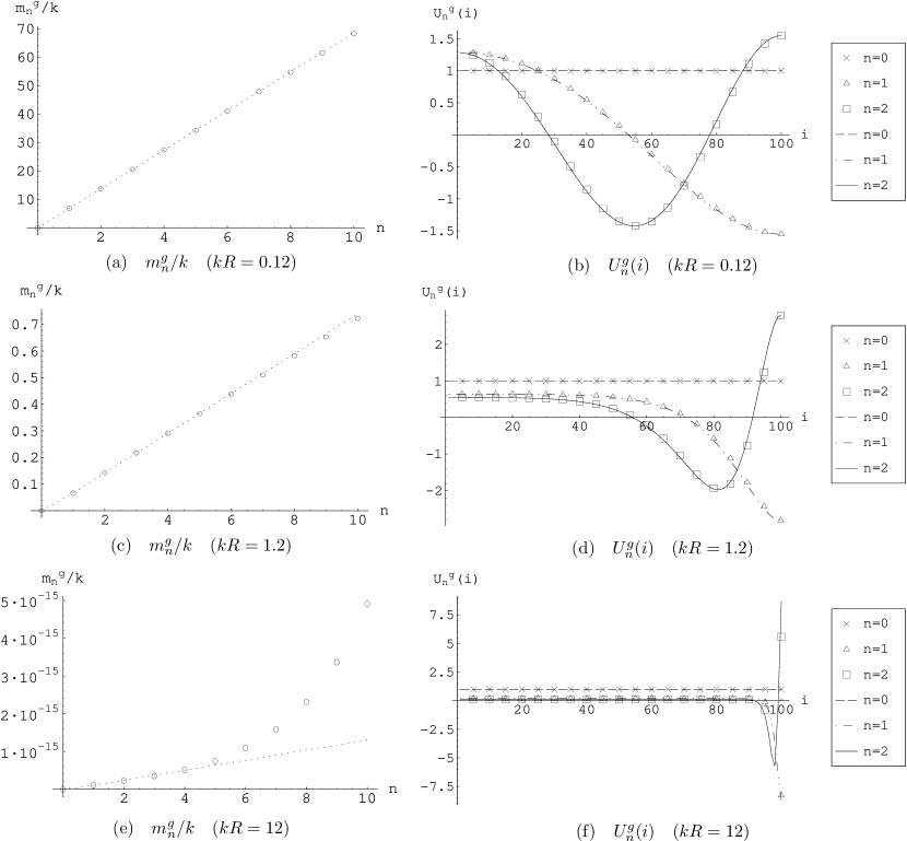
Figure 2: The mass eigenvalues and eigenvectors of the matrix $D_{1/2}$ for vector fields in the cases $\,kL/2\pi=$ 0.12, 1.2 and 12. We take the total number of gauge groups as $N=100$. (a), (c), and (e) show the eigenvalues $m_{n}^{g}$ for each $kL$ with the symbols $\circ$. The corresponding KK mass spectrum of the continuum RS theory is also depicted by the dotted lines. (b), (d), and (f) show the eigenvectors $U^{g}_{n}(i)$ for each $kL$ with the symbols $\times$, $\triangle$, and $\Box$. The corresponding KK wave function of the continuum RS theory is also depicted by the lines. For the continuum cases, the horizontal axis is $gvy$. The wave functions plotted here are normalized by the zero-mode ones.

For fermion fields, there is another interesting issue to be examined. It is the localization behavior via dependence on the mass parameters $c$, which was discussed in Sec.2.2. We show the $c$ dependence of the zero-mode wave function $U^{f}_{0}(i)$ in Fig. 3.

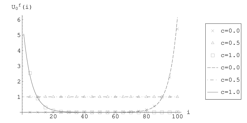
Figure 3: Typical behavior of the massless eigenvector $U^{f}_{0}(i)$ for fermions with mass parameter $c$ (denoted by the symbols $\times$, $\triangle$, and $\Box$). The total number of gauge groups is taken as $N=100$. The corresponding zero-mode wave functions in the continuum RS theory are depicted by the lines. The case $c=1/2$ is the conformal limit where the massless mode is not localized.

The figure indicates that the zero-mode wave functions surely give the expected localization nature of the continuum RS limit [Eq. (90) in the Appendix]. We find that the values of the wave functions are exponentially suppressed at the tail of localization profile even with a finite number of gauge groups. The profiles of massive modes can also be reproduced.

3.2 Yukawa hierarchy from 4D

Now we apply our formulation to phenomenological problems in four dimensions. Let us use the localization behavior, which has been shown above, to obtain the Yukawa hierarchy. This issue has been studied in the 5D RS framework [3, 5]. We consider a model corresponding to the (supersymmetric) standard model in the bulk. The Yukawa couplings for quarks are given by

$${\cal L}_{\rm Yukawa} = \sum_{i=1}^{N}\left((y_{u}^{ab})_{i}\,q^{i}_{a}H^{i}_{u}u^{i}_{b}+(y_{d}^{ab})_{i}\,q^{i}_{a}H^{i}_{d}d^{i}_{b}\right)+\textrm{H.c.},$$ (60)

where $q$, $u$, and $d$ denote the left-handed quarks and the right-handed up and down quarks, respectively, and $a,b$ are the family indices. For simplicity, we study a supersymmetric case and introduce two types of Higgs scalars $H^{i}_{u}$ and $H^{i}_{d}$. Then the mass parameters of the Higgs scalars satisfy Eq. (48) and they are denoted by $c^{H_{u,d}}$ in the following. Similarly, the quark behaviors are described by their mass parameters $c^{q,u,d}$. We assume $(y_{u,d}^{ab})_{i}\sim{\cal O}(1)$. Generally, in supersymmetric 5D models, Yukawa couplings such as Eq. (60) are prohibited by 5D supersymmetry. However, since the present model is 4D, one may apply 5D-like results to Yukawa couplings without respecting 5D consistency. This is one of the benefits of our scheme.

We are now interested in the zero-mode part of Eq. (60), which generates the following mass terms

$${\cal L}_{\rm Yukawa} = Y_{u}^{ab}\tilde{q}^{0}_{a}\langle\tilde{H}^{0}_{u}\rangle\tilde{u}^{0}_{b}+Y_{d}^{ab}\tilde{q}^{0}_{a}\langle\tilde{H}^{0}_{d}\rangle\tilde{d}^{0}_{b}\,+\textrm{H.c.},$$ (61)

where the fields with tildes $\tilde{q}^{j}$ stand for the $j$th mass eigenstate given by $\tilde{q}^{j}=\sum_{i=1}^{N}U_{j}^{q}(i)\,q^{i}$ (similarly for $u$, $d$, and $H_{u,d}$). The effective Yukawa couplings are

$$Y_{u}^{ab} = y_{u}^{ab}\sum_{i=1}^{N}\,U_{0}^{H_{u}}(i)\,U_{0}^{q_{a}}(i)\,U_{0}^{u_{b}}(i),$$ (62)

and similarly for $Y_{d}$. A typical behavior of $U_{0}(i)$ is shown in Fig. 3 for several values of the bulk mass parameter $c$. In Fig. 4, we show the behaviors of the zero-mode Yukawa couplings $Y_{u,d}$ against the quark mass parameters. Two limiting cases with $c^{H_{u,d}}=0$ and 1 are shown. The former corresponds to a bulk Higgs scalar localized at $y=L/2$ and the latter to one at $y=0$ in the continuum RS limit. From the figures, we see that if there is a ${\cal O}(1)$ difference of mass ratio among the generations, it generates a large hierarchy between Yukawa couplings. Combined with the mechanisms that control mass parameters discussed in the next section, one obtains a hierarchy without symmetries within the four-dimensional framework.

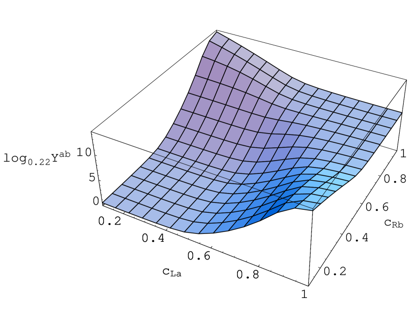
(a) $c^{H_{u,d}}=0$

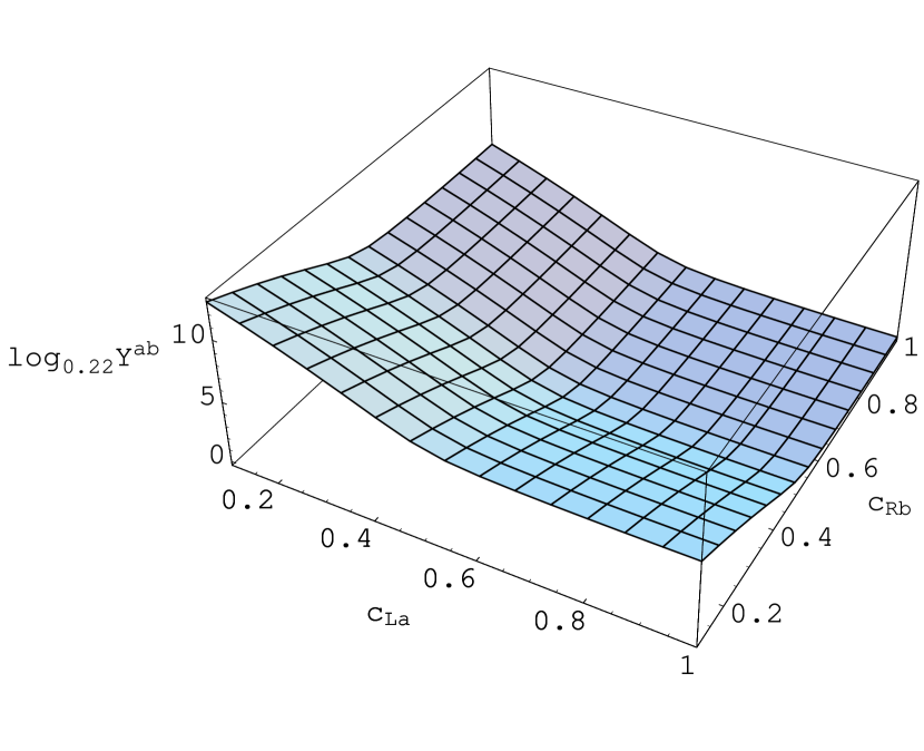
(b) $c^{H_{u,d}}=1$

     

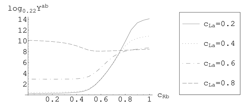
(c) $c^{H_{u,d}}=0$

     

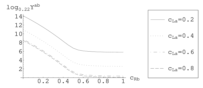
(d) $c^{H_{u,d}}=1$

Figure 4: The quark mass $c^{q}$ ($\equiv c_{L}$) and $c^{u,d}$ ($\equiv c_{R}$) dependences of the zero-mode Yukawa coupling $Y^{ab}$ with $kL/2\pi=10.83$ and $N=20$. The mass parameters of the Higgs scalars $c^{H_{u,d}}$ are taken to be $0$ in (a) and (c), and $1$ in (b) and (d).

In the case of $c^{H_{u,d}}=1$, the Yukawa coupling depends exponentially on the quark bulk mass parameters $c^{q,u,d}$ when $c^{q,u,d}<0.5$. This implies that if $c^{q,u,d}$ exist in this region one obtains the following form of the Yukawa matrices:

$$\pmatrix{\lambda^{n_{aa}}&\lambda^{n_{ab}}\cr\lambda^{n_{ba}}&\lambda^{n_{bb}}},$$ (63)

where their exponents satisfy

$$n_{aa}+n_{bb}\,=\,n_{ab}+n_{ba}.$$ (64)

This form is similar to that obtained by the Froggatt-Nielsen mechanism [15] with a ${\rm U}(1)$ symmetry. As an illustration, let us take the following mass parameters

$$c^{q_{1,2,3}} = (0.36,\ 0.42,\ 1.00),$$

$$c^{u_{1,2,3}} = (0.36,\ 0.42,\ 1.00),$$ (65)

$$c^{d_{1,2,3}} = (0.42,\ 1.00,\ 1.00),$$

$$c^{H^{u,d}} = 1,$$

and $N=20$ and $kR=10.83$, which generates the low-energy Yukawa matrices

$$Y_{u}^{ab}\,\simeq\,\pmatrix{\lambda^{6}&\lambda^{5}&\lambda^{3}\cr\lambda^{5}&\lambda^{4}&\lambda^{2}\cr\lambda^{3}&\lambda^{2}&1},\qquad Y_{d}^{ab}\,\simeq\,\pmatrix{\lambda^{5}&\lambda^{3}&\lambda^{3}\cr\lambda^{4}&\lambda^{2}&\lambda^{2}\cr\lambda^{2}&1&1},$$ (66)

where $\lambda=0.22$. This pattern of quark mass textures leads to realistic quark masses and mixing angles [16] with a large value of the ratio $\langle\tilde{H}_{u}^{0}\rangle/\langle\tilde{H}_{d}^{0}\rangle$. If the above analysis were extended to SU(5) grand unified theory, realistic lepton masses and mixing may be derived. Other forms of Yukawa matrices that may be realized by the Froggatt-Nielsen mechanism are easily incorporated in our formulation.

For more complicated patterns of mass parameters, we could realize Yukawa matrices that are different from those derived from the Froggatt-Nielsen mechanism. In general, off-diagonal entries tend to be rather suppressed, that is, we have

$$n_{aa}+n_{bb}\,\leq\,n_{ab}+n_{ba}$$ (67)

for the Yukawa matrix (63). Such a form may lead to realistic fermion masses and mixing angles. For example, one could derive the Yukawa matrix

$$Y^{ab}\,\simeq\,\pmatrix{0&\lambda^{4}&0\cr\lambda^{4}&\lambda^{3}&\lambda^{3}\cr 0&\lambda^{3}&1}$$ (68)

if initial values of $(y^{11})_{i}$ are sufficiently suppressed. In this case, the $2\times 2$ submatrix for the second and third generations does not satisfy Eq. (64). The Yukawa matrix (68) may be relevant to the down-quark sector, indeed studied in Ref. [17]. We do not pursue further systematic studies on these types of Yukawa matrices in this paper.

4 Toward dynamical realization

We have shown that 4D models with nonuniversal VEVs and gauge and other couplings can describe 5D physics on curved backgrounds, including the RS model with an exponential warp factor. In the continuum 5D theory, this factor is derived as a solution of the equation of motion for gravity. On the other hand, in the 4D viewpoint, warped geometries are generated by taking the couplings and VEVs as appropriate forms. In the previous sections, we have just assumed their typical forms and examined its consequences. If one could identify how to control these couplings by the underlying dynamics, the resultant 4D theories turn out to provide attractive schemes to discuss low-energy physics such as tiny coupling constants.

First we consider the scalar VEVs $\langle Q_{i}\rangle=v_{i}$. A simple way to dynamically control them is to introduce additional strongly coupled gauge theories [9]. Consider the following set of asymptotically free gauge theories:

$$A_{\mu}^{i} : {\rm SU}(n)_{i}\textrm{ gauge field }(g,\Lambda),$$ (69)

$$\hat{A}_{\mu}^{i} : {\rm SU}(m)_{i}\textrm{ gauge field }(\hat{g}_{i},\hat{\Lambda}_{i}),$$ (70)

where $\Lambda$ and $\hat{\Lambda}_{i}$ denote the dynamical scales. We have, for simplicity, assumed common values of $g$ and $\Lambda$ for all ${\rm SU}(n)_{i}$. In addition, two types of fermions are introduced:

$$\xi^{i}\;:\;(n,\bar{m},1),\qquad\bar{\xi}^{i}\;:\;(1,m,\bar{n}),$$ (71)

where their representations under ${\rm SU}(n)_{i}\times{\rm SU}(m)_{i}\times{\rm SU}(n)_{i+1}$ gauge groups are shown in parentheses. If $\hat{\Lambda}_{i}\gg\Lambda$, the ${\rm SU}(m)_{i}$ theories are confined at a higher scale than ${\rm SU}(n)_{i}$, and the fermion bilinear composite scalars $Q_{i}\sim\xi^{i}\bar{\xi}^{i}$ appear. Their VEVs $v_{i}$ are given by the dynamical scales $\hat{\Lambda}_{i}$ of the ${\rm SU}(m)_{i}$ gauge theories through a dimensional transmutation as

$$\langle Q_{i}\rangle\,\equiv\,v_{i}\,\simeq\,\hat{\Lambda}_{i}\,=\,\mu\,e^{1/2\hat{\beta}\hat{g}_{i}^{2}(\mu)},$$ (72)

where $\hat{\beta}$ is a universal one-loop gauge beta function for ${\rm SU}(m)_{i}$ ($\hat{\beta}<0$). The gauge couplings $\hat{g}_{i}$ generally take different values and thus lead to different values of $v_{i}$. For example, a linear dependence of $1/\hat{g}_{i}^{2}$ on the index $i$ is amplified to an exponential behavior of $v_{i}$. That is,

$$\frac{1}{\hat{g}_{i}^{2}(\mu)}\,=\,-2\hat{\beta}\biggl{(}\frac{k}{gv}\biggr{)}i\quad\longleftrightarrow\quad v_{i}\,=\,ve^{-ki/gv},$$ (73)

which reproduces the bulk fields on the RS background as shown before. The index dependences of the gauge couplings are actually generic situations, and may also be controlled, for example, by some mechanism fixing dilatons or the radiatively induced kinetic terms discussed below. A supersymmetric extension of the above scenario is achieved with quantum-deformed moduli spaces [12].

Another mechanism that dynamically induces nonuniversal VEVs is obtained in supersymmetric cases. Consider the gauge group $\prod_{i}{\rm U}(1)_{i}$ and the chiral superfields $Q_{i}$ with charges $(+1,-1)$ under ${\rm U}(1)_{i}\times{\rm U}(1)_{i+1}$. It is assumed that the scalar components $q_{i}$ of $Q_{i}$ develop their VEVs $\langle q_{i}\rangle=v_{i}$. The $D$ term of each ${\rm U}(1)_{i}$ is given by

$$D_{i}\,=\,\epsilon_{i}+|q_{i}|^{2}-|q_{i-1}|^{2}+\cdots,$$ (74)

where $\epsilon_{i}$ is the coefficient of the Fayet-Iliopoulos (FI) term, and the ellipsis denotes contributions from other fields charged under ${\rm U}(1)_{i}$, which are assumed not to have VEVs. Given nonvanishing FI terms, $\epsilon_{i}\neq 0$, the $D$-flatness conditions mean

$$v_{i-1}^{2}\,=\,v_{i}^{2}+\epsilon_{i},$$ (75)

and nonuniversal VEVs $v_{i}$ are indeed realized. In this case, the dynamical origin of nonuniversal VEVs is the nonvanishing FI terms. These may be generated at the loop level. Furthermore, if the matter content is different for each gauge theory, the $\epsilon_{i}$ themselves have complicated forms.

Above, we supposed that the charges of $Q_{i}$ are $(+1,-1)$ under ${\rm U}(1)_{i}\times{\rm U}(1)_{i+1}$. Alternatively, if $Q_{i}$ have charges $(M,-M)$ under ${\rm U}(1)_{i}\times{\rm U}(1)_{i+1}$ and other matter fields have integer charges, the gauge symmetry $\prod_{i}{\rm U}(1)_{i}$ is broken to the product of a diagonal ${\rm U}(1)$ gauge symmetry and the discrete gauge symmetry $\prod_{i}(Z_{M})_{i}$. Such discrete gauge symmetry would be useful for phenomenology [18].

Models with nonuniversal gauge couplings $g_{i}$ are also interesting in the sense that they can describe the localization of massless vector fields. A nonuniversality of gauge couplings is generated, e.g., in the case that the ${\rm SU}(n)_{i}$ gauge theories have different matter content from each other. Then radiative corrections to gauge couplings and their renormalization-group running become nonuniversal, even if their initial values are equal.

This fact is also applicable to the above-mentioned mechanism for nonuniversal $v_{i}$. Suppose that the ${\rm SU}(m)_{i}$ theory contains ($2m+i$) vectorlike quarks which decouple at $v$. The gauge couplings $\hat{g}_{i}(v)$ are then determined by

$$\frac{1}{\hat{g}_{i}^{2}(v)}\;=\;\frac{i}{8\pi^{2}}\ln\biggl{(}\frac{\Lambda^{\prime}}{v}\biggr{)},$$ (76)

where we have assumed that the ${\rm SU}(m)_{i}$ theories are strongly coupled at a high-energy scale $\Lambda^{\prime}$ ($>v$). Tuning of the relevant matter content thus generates the desired linear dependence of $1/\hat{g}_{i}^{2}$. With these radiatively induced couplings (76) at hand, the VEVs are determined from Eq. (72):

$$v_{i}\;=\;v\biggl{(}\frac{v}{\Lambda^{\prime}}\biggr{)}^{i/2m}.$$ (77)

5 Conclusion

We have formulated 4D models that provide 5D field theories on generic warped backgrounds. The warped geometries are achieved with generic values of symmetry-breaking VEVs, gauge couplings, and other couplings in the models. We focused on field localization behaviors along the index space of gauge theory (the fifth dimension in the continuum limit), which is realized by taking relevant choices of the mass parameters.

As a good and simple application, we constructed 4D models corresponding to bulk field theories on the AdS₅ Randall-Sundrum background. The localized wave functions of massless modes are completely reproduced with a finite number of gauge groups. In addition, the exponentially suppressed spectrum of the KK modes is also generated. These results imply that most properties of brane world models can be obtained within 4D gauge theories. Supersymmetric extensions were also investigated. In 5D warped models, the bulk and boundary mass terms of spinors and scalars satisfy complicated forms imposed by supersymmetry on the RS background. However, we show in our formalism that these forms of the mass terms are derived from a 4D global supersymmetric model on a flat background.

As an application of our 4D formulation, we derived hierarchical forms of Yukawa couplings. The zero modes of scalars and spinors with different masses have different wave-function profiles as in the 5D RS cases. Therefore by varying the ${\cal O}(1)$ mass parameters for each generation, one can obtain realistic Yukawa matrices with a large hierarchy from the overlaps of the wave functions in a purely 4D framework. Other phenomenological issues such as proton stability, grand unified theory (GUT) symmetry breaking, and supersymmetry breaking can also be discussed.

The conditions on the model parameters should be explained by some dynamical mechanisms if one considers the models from a fully 4D viewpoint. One interesting way is to include additional strongly coupled gauge theories. In this case, a small ${\cal O}(1)$ difference between gauge couplings is converted to exponential profiles of symmetry-breaking VEVs via dimensional transmutation, and indeed generates a warp factor of the RS model. A difference of gauge couplings is achieved by, for example, the dynamics controlling dilatons, or radiative corrections to gauge couplings. Supersymmetrizing models provide a mechanism for dynamically realizing nonuniversal VEVs with $D$-flatness conditions.

Our formulation makes sense not only from the 4D points of view but also as a lattice-regularized 5D theory. In this sense, effects such as the AdS/conformal field theory (CFT) correspondence might be clearly seen with our formalism. As another application, it can be applied to construct various types of curved backgrounds and bulk or boundary masses. For example, we discussed massless vector localization by varying the gauge couplings $g_{i}$. Furthermore, one might consider models in which some fields are charged under only some of the gauge groups. These seem not like bulk or brane fields, but “quasi-bulk” fields. Applications including these phenomena will be studied elsewhere.

Acknowledgment

This work is supported in part by the Japan Society for the Promotion of Science under the Postdoctoral Research Program (Grants No. $08557$ and No. $07864$) and a Grant-in-Aid for Scientific Research from the Ministry of Education, Science, Sports and Culture of Japan (No. $14540256$).

Appendix.  Bulk fields in AdS₅

Here we briefly review the field theory on a RS background, following Ref. [3]. One of the original motivations for introducing a warped extra dimension by Randall and Sundrum is to provide the weak Planck mass hierarchy via the exponential factor in the space-time metric. This factor is called “warp factor,” and the bulk space a “warped extra dimension”. Such a nonfactorizable geometry with a warp factor distinguishes the RS brane world from others.

Consider the fifth dimension $y$ compactified on an orbifold $S^{1}/{\bf Z}_{2}$ with radius $R$ and two three-branes at the orbifold fixed points $y=0$ and $y=L/2\equiv\pi R$. The Einstein equation for this five-dimensional setup leads to the solution [1]

$$ds^{2}\,=\,e^{-2\sigma}\eta_{\mu\nu}dx^{\mu}dx^{\nu}-dy^{2},\qquad\sigma\,=\,k|y|,$$ (78)

where $k$ is a constant with mass dimension $1$. Let us study a vector field $A_{M}$, a Dirac fermion $\Psi$, and a complex scalar $\phi$ in the bulk specified by the background metric (78). The 5D action is given by

$$S_{5}\,=\,\int d^{4}x\int_{0}^{\pi R}dy\sqrt{-g}\,\Bigg{[}\frac{-1}{4g^{2}_{5}}F^{2}_{MN}+\left|\partial_{M}\phi\right|^{2}+i\bar{\Psi}\gamma^{M}D_{M}\Psi-m^{2}_{\phi}|\phi|^{2}-m_{\Psi}\bar{\Psi}\Psi\Bigg{]},$$ (79)

where $\gamma_{M}=(\gamma_{\mu},i\gamma_{5})$ and the covariant derivative is $D_{M}=\partial_{M}+\Gamma_{M}$ where $\Gamma_{M}$ is the spin connection given by $\Gamma_{\mu}=i\gamma_{5}\gamma_{\mu}\sigma^{\prime}/2$ and $\Gamma_{4}=0$. From the transformation properties under ${\bf Z}_{2}$ parity, the mass parameters of scalar and fermion fields are parametrized as

$$m^{2}_{\phi} = ak^{2}+\frac{b}{2}\sigma^{\prime\prime},$$ (80)

$$m_{\Psi} = c\sigma^{\prime},$$ (81)

where $a$, $b$, and $c$ are dimensionless parameters.

Referring to [3], the vector, scalar and spinor fields are cited together using the single notation $\Phi=\{A_{\mu},\ \phi,\ e^{-2\sigma}\Psi_{L,R}\}$. The KK mode expansion is performed as

$$\Phi(x^{\mu},y)\,=\,{1\over\sqrt{2\pi R}}\sum_{n=0}^{\infty}\Phi^{(n)}(x^{\mu})f_{n}(y).$$ (82)

By solving the equations of motion, the eigenfunction $f_{n}$ is given by

$$f_{n}(y) = \frac{e^{s\sigma/2}}{N_{n}}\left[J_{\alpha}\left(\frac{m_{n}}{k}e^{\sigma}\right)+b_{\alpha}(m_{n})\,Y_{\alpha}\left(\frac{m_{n}}{k}e^{\sigma}\right)\right],$$ (83)

where $\alpha=\sqrt{(s/2)^{2}+M^{2}_{\Phi}/k^{2}}$, $s=\{2,\ 4,\ 1\}$, and $M^{2}_{\Phi}=\{0,\ ak^{2},\ c(c\,\pm\,1)k^{2}\}$ for each component in $\Phi$. $N_{n}$ is the normalization factor and $J_{\alpha}$ and $Y_{\alpha}$ are the Bessel functions. The corresponding KK spectrum $m_{n}$ is obtained by solving

$$b_{\alpha}(m_{n})\,=\,b_{\alpha}(m_{n}e^{\pi kR}).$$ (84)

A supersymmetric extension of this scenario was discussed in [3, 4]. The on-shell field content of a vector supermultiplet is $(A_{M},\lambda_{i},\Sigma)$ where $A_{M}$, $\lambda_{i}~{}(i=1,2)$, and $\Sigma$ are the vector, two Majorana spinors, and a real scalar in the adjoint representation, respectively. Also a hypermultiplet consists of $(H_{i},\Psi)$, where $H_{i}$ $(i=1,2)$ are two complex scalars and $\Psi$ is a Dirac fermion. By requiring the action (79) to be invariant under supersymmetric transformation on the warped background, one finds that the five-dimensional masses of the scalar and spinor fields have to satisfy

$$m^{2}_{\Sigma} = -4k^{2}+2\sigma^{\prime\prime},$$ (85)

$$m_{\lambda} = \frac{1}{2}\sigma^{\prime},$$ (86)

$$m^{2}_{H^{1,2}} = \left(c^{2}\pm c-\frac{15}{4}\right)k^{2}+\left(\frac{3}{2}\mp c\right)\sigma^{\prime\prime},$$ (87)

$$m_{\Psi} = c\sigma^{\prime},$$ (88)

where $c$ remains as an arbitrary dimensionless parameter. That is, $a=-4$, $b=2$, and $c=1/2$ for vector multiplets and $a=c^{2}\pm c-15/4$ and $b=3/2\mp c$ for hypermultiplets. There is no freedom to choose the bulk masses for vector supermultiplets and only one freedom parametrized by $c$ for the bulk hypermultiplets. It should be noted that in warped 5D models fields contained in the same supermultiplet have different bulk and boundary masses. That is in contrast with the flat case.

The $Z_{2}$ even components in supermultiplets have massless modes with the following wave functions:

$$\frac{1}{\sqrt{2\pi R}}~{}~{} \textrm{ for }\;V^{(0)}_{\mu}\,\textrm{ and }\,\lambda^{1\,(0)}_{L},$$ (89)

$$\frac{e^{(1/2-c)\sigma}}{N_{0}\sqrt{2\pi R}} \textrm{ for }\;H^{1\,(0)}\,\textrm{ and }\,\Psi^{(0)}_{L}.$$ (90)

The subscript $L$ means the left-handed ($Z_{2}$ even) component. The massless vector multiplet has a flat wave function in the extra dimension. On the other hand, the wave function for massless chiral multiplets involves a $y$-dependent contribution from the space-time metric, which induces a localization of the zero modes. The zero modes with masses $c>1/2$ and $c<1/2$ localize at $y=0$ and $y=\pi R$, respectively. The case with $c=1/2$ corresponds to the conformal limit where the kinetic terms of the zero modes are independent of $y$.

References

- [1] L. Randall and R. Sundrum, Phys. Rev. Lett. 83, 3370 (1999) [hep-ph/9905221]; Phys. Rev. Lett. 83, 4690 (1999) [hep-th/9906064].
- [2] W. D. Goldberger and M. B. Wise, Phys. Rev. D 60, 107505 (1999) [hep-ph/9907218]; Phys. Rev. Lett. 83, 4922 (1999) [hep-ph/9907447]; H. Davoudiasl, J. L. Hewett and T. G. Rizzo, Phys. Lett. B 473, 43 (2000) [hep-ph/9911262]; A. Pomarol, Phys. Lett. B 486, 153 (2000) [hep-ph/9911294]; S. Chang, J. Hisano, H. Nakano, N. Okada and M. Yamaguchi, Phys. Rev. D 62, 084025 (2000) [hep-ph/9912498]; B. Bajc and G. Gabadadze, Phys. Lett. B 474, 282 (2000) [hep-th/9912232]; E. Shuster, Nucl. Phys. B 554, 198 (1999) [hep-th/9902129].
- [3] T. Gherghetta and A. Pomarol, Nucl. Phys. B 586, 141 (2000) [hep-ph/0003129].
- [4] T. Gherghetta and A. Pomarol, Nucl. Phys. B 602, 3 (2001) [hep-ph/0012378].
- [5] S. J. Huber and Q. Shafi, Phys. Lett. B 498, 256 (2001) [hep-ph/0010195].
- [6] H. Abe and T. Inagaki, Phys. Rev. D 66, 085001 (2002) [hep-ph/0206282]. H. Abe, K. Fukazawa and T. Inagaki, Prog. Theor. Phys. 107, 1047 (2002) [hep-ph/0107125]; H. Abe, T. Inagaki and T. Muta, in Fluctuating Paths and Fields, edited by W. Janke, A. Pelster, H.-J. Schmidt, and M. Bachmann (World Scientific, Singapore, 2001) [hep-ph/0104002].
- [7] I. I. Kogan, S. Mouslopoulos, A. Papazoglou and G. G. Ross, Nucl. Phys. B 615, 191 (2001) [hep-ph/0107307].
- [8] S. Dimopoulos, S. Kachru, N. Kaloper, A. E. Lawrence and E. Silverstein, Phys. Rev. D 64, 121702 (2001) [hep-th/0104239].
- [9] N. Arkani-Hamed, A. G. Cohen and H. Georgi, Phys. Rev. Lett. 86, 4757 (2001) [hep-th/0104005].
- [10] C. T. Hill, S. Pokorski and J. Wang, Phys. Rev. D 64, 105005 (2001) [hep-th/0104035].
- [11] H. C. Cheng, C. T. Hill, S. Pokorski and J. Wang, Phys. Rev. D 64, 065007 (2001) [hep-th/0104179]; A. Sugamoto, Prog. Theor. Phys. 107, 793 (2002) [hep-th/0104241]; H. C. Cheng, C. T. Hill and J. Wang, Phys. Rev. D 64, 095003 (2001) [hep-ph/0105323]; N. Arkani-Hamed, A. G. Cohen and H. Georgi, Phys. Lett. B 513, 232 (2001) [hep-ph/0105239]; H. C. Cheng, D. E. Kaplan, M. Schmaltz and W. Skiba, Phys. Lett. B 515, 395 (2001) [hep-ph/0106098]; M. Bander, Phys. Rev. D 64, 105021 (2001) [hep-th/0107130]; C. Csaki, G. D. Kribs and J. Terning, Phys. Rev. D 65, 015004 (2002) [hep-ph/0107266]; H. C. Cheng, K. T. Matchev and J. Wang, Phys. Lett. B 521, 308 (2001) [hep-ph/0107268]; N. Arkani-Hamed, A. G. Cohen and H. Georgi, hep-th/0108089; C. T. Hill, Phys. Rev. Lett. 88, 041601 (2002) [hep-th/0109068]; N. Arkani-Hamed, A. G. Cohen and H. Georgi, JHEP 0207, 020 (2002) [hep-th/0109082]; I. Rothstein and W. Skiba, Phys. Rev. D 65, 065002 (2002) [hep-th/0109175]; T. Kobayashi, N. Maru and K. Yoshioka, hep-ph/0110117; N. Arkani-Hamed, A. G. Cohen, D. B. Kaplan, A. Karch and L. Motl, hep-th/0110146; C. Csaki, J. Erlich, V. V. Khoze, E. Poppitz, Y. Shadmi and Y. Shirman, Phys. Rev. D 65, 085033 (2002) [arXiv:hep-th/0110188]; G. C. Cho, E. Izumi and A. Sugamoto, hep-ph/0112336; E. Witten, hep-ph/0201018; W. Skiba and D. Smith, Phys. Rev. D 65, 095002 (2002) [hep-ph/0201056]; R. S. Chivukula and H. J. He, Phys. Lett. B 532, 121 (2002) [hep-ph/0201164]; N. Arkani-Hamed, A. G. Cohen, T. Gregoire and J. G. Wacker, JHEP 0208, 020 (2002) [hep-ph/0202089]; K. Lane, Phys. Rev. D 65, 115001 (2002) [hep-ph/0202093]; Z. Berezhiani, A. Gorsky and I. I. Kogan, JETP Lett. 75, 530 (2002); Pisma Zh. Eksp. Teor. Fiz. 75, 646 (2002) [hep-th/0203016]; A. Falkowski, C. Grojean and S. Pokorski, Phys. Lett. B 535, 258 (2002) [hep-ph/0203033]; C. T. Hill and A. K. Leibovich, Phys. Rev. D 66, 016006 (2002) [hep-ph/0205057].
- [12] C. Csaki, J. Erlich, C. Grojean and G. D. Kribs, Phys. Rev. D 65, 015003 (2002) [hep-ph/0106044].
- [13] K. Sfetsos, Nucl. Phys. B 612, 191 (2001) [hep-th/0106126].
- [14] A. Kehagias and K. Tamvakis, Phys. Lett. B 504, 38 (2001) [hep-th/0010112].
- [15] C. D. Froggatt and H. B. Nielsen, Nucl. Phys. B 147, 277 (1979).
- [16] G. Altarelli and F. Feruglio, Phys. Lett. B 451, 388 (1999) [hep-ph/9812475].
- [17] P. Ramond, R. G. Roberts and G. G. Ross, Nucl. Phys. B 406, 19 (1993) [hep-ph/9303320].
- [18] L. E. Ibanez and G. G. Ross, Nucl. Phys. B 368, 3 (1992); Phys. Lett. B 260, 291 (1991).
- [19] J. Wess and J. Bagger, Supersymmetry and Supergravity (Princeton University Press, Princeton, NJ, 1992)