DESY 02-005 hep-ph/0205254 May 2002 Helicity Analysis of the Decays $B\to K^{*}\ell^{+}\ell^{-}$ and $B\to\rho\ell\nu_{\ell}$ in the Large Energy Effective Theory

Abstract

We calculate the independent helicity amplitudes in the decays $B\to K^{*}\ell^{+}\ell^{-}$ and $B\to\rho\ell\nu_{\ell}$ in the so-called Large-Energy-Effective-Theory (LEET). Taking into account the dominant $O(\alpha_{s})$ and $SU(3)$ symmetry-breaking effects, we calculate various Dalitz distributions in these decays making use of the presently available data and decay form factors calculated in the QCD sum rule approach. Differential decay rates in the dilepton invariant mass and the Forward-Backward asymmetry in $B\to K^{*}\ell^{+}\ell^{-}$ are worked out. We also present the decay amplitudes in the transversity basis which has been used in the analysis of data on the resonant decay $B\to K^{*}J/\psi(\to\ell^{+}\ell^{-})$. Measurements of the ratios $R_{i}(s)\equiv d\Gamma_{H_{i}}(s)(B\to K^{*}\ell^{+}\ell^{-})/d\Gamma_{H_{i}}(s)(B\to\rho\ell\nu_{\ell})$, involving the helicity amplitudes $H_{i}(s)$, $i=0,+1,-1$, as precision tests of the standard model in semileptonic rare $B$-decays are emphasized. We argue that $R_{0}(s)$ and $R_{-}(s)$ can be used to determine the CKM ratio $|V_{ub}|/|V_{ts}|$ and search for new physics, where the later is illustrated by supersymmetry.

1 Introduction

Rare $B$ decays involving flavour-changing-neutral-current (FCNC) transitions, such as $b\to s\gamma$ and $b\to s\ell^{+}\ell^{-}$, have received a lot of theoretical interest [1]. First measurements of the decay $B\to X_{s}\gamma$ were reported by the CLEO collaboration [2]. These decays are now being investigated more precisely in experiments at the B factories. The current world average based on the improved measurements by the CLEO [3], ALEPH [4] and BELLE [5] collaborations, ${\cal B}(B\to X_{s}\gamma)=(3.22\pm 0.40)\times 10^{-4}$, is in good agreement with the estimates of the standard model (SM) [6, 7, 8], which we shall take as ${\cal B}(B\to X_{s}\gamma)=(3.50\pm 0.50)\times 10^{-4}$, reflecting the parametric uncertainties dominated by the scheme-dependence of the quark masses. The decay $B\to X_{s}\gamma$ also provides useful constraints on the parameters of the supersymmetric theories, which in the context of the minimal supersymmetric standard model (MSSM) have been recently updated in [9].

Exclusive decays involving the $b\to s\gamma$ transition are best exemplified by the decay $B\to K^{*}\gamma$, which have been measured with a typical accuracy of $\pm 10\%$, the current branching ratios being [3, 10, 11] ${\cal B}(B^{\pm}\to K^{*\pm}\gamma)=(3.82\pm 0.47)\times 10^{-5}$ and ${\cal B}(B^{0}\to K^{*0}\gamma)=(4.44\pm 0.35)\times 10^{-5}$. These decays have been analyzed recently [12, 13, 14], by taking into account $O(\alpha_{s})$ corrections, henceforth referred to as the next-to-leading-order (NLO) estimates, in the large-energy-effective-theory (LEET) limit [15, 16]. As this framework does not predict the decay form factors, which have to be supplied from outside, consistency of NLO-LEET estimates with current data constrains the magnetic moment form factor in $B\to K^{*}\gamma$ in the range $T_{1}^{K^{*}}(0)=0.27\pm 0.04$. These values are somewhat lower than the corresponding estimates in the lattice-QCD framework, yielding [17] $T_{1}^{K^{*}}(0)=0.32^{+0.04}_{-0.02}$, and in the light cone QCD sum rule approach, which give typically $T_{1}^{K^{*}}(0)=0.38\pm 0.05$ [19, 18]. (Earlier lattice-QCD results on $B\to K^{*}\gamma$ form factors are reviewed in [20].) It is imperative to check the consistency of the NLO-LEET estimates, as this would provide a crucial test of the ideas on QCD-factorization, which have been formulated in the context of non-leptonic exclusive $B$-decays [21], but which have also been invoked in the study of exclusive radiative and semileptonic $B$-decays [12, 13, 14]. The decays $B\to\rho\gamma$ and $B\to K^{*}\gamma$ provide a good consistency check of this framework, with the branching ratios, the isospin-violating ratio $\frac{\Gamma(B^{\pm}\to\rho^{\pm}\gamma)}{2\Gamma(B^{0}\to\rho^{0}\gamma)}-1$ and direct CP-violating asymmetries, such as ${\cal A}(\rho^{\pm}\gamma)\equiv\frac{{\cal B}(B^{-}\to\rho^{-}\gamma)-{\cal B}(B^{+}\to\rho^{+}\gamma)}{{\cal B}(B^{-}\to\rho^{-}\gamma)+{\cal B}(B^{+}\to\rho^{+}\gamma)}$, being the quantities of interest [14, 12]. Likewise, isospin-violation in the decays $B\to K^{*}\gamma$, defined as $\Delta_{0-}=\frac{\Gamma(B^{0}\to K^{*0}\gamma)-\Gamma(B^{-}\to K^{*-}\gamma)}{\Gamma(B^{0}\to K^{*0}\gamma)+\Gamma(B^{-}\to K^{*-}\gamma)}$ and its charge conjugate $\Delta_{0+}$, will also test this framework [22].

The exclusive decays $B\to K^{*}\ell^{+}\ell^{-}$, $\ell^{\pm}=e^{\pm},\mu^{\pm}$ have also been studied in the NLO-LEET approach in [23, 13]. In this case, the LEET symmetry brings an enormous simplicity, reducing the number of independent form factors from seven to only two, corresponding to the transverse and longitudinal polarization of the virtual photon in the underlying process $B\to K^{*}\gamma^{*}$, called hereafter $\xi_{\perp}^{K^{*}}(q^{2})$ and $\xi_{||}^{K^{*}}(q^{2})$. The same symmetry reduces the number of independent form factors in the decays $B\to\rho\ell\nu_{\ell}$ from four to two. Moreover, in the $q^{2}$-range where the large energy limit holds, the two set of form factors are equal to each other, up to $SU(3)$-breaking corrections, which are already calculated in specific theoretical frameworks. Thus, knowing $V_{ub}$ precisely, one can make theoretically robust predictions for the rare $B$-decay $B\to K^{*}\ell^{+}\ell^{-}$ from the measured $B\to\rho\ell\nu_{\ell}$ decay in the SM. The LEET symmetries are broken by QCD interactions and the leading $O(\alpha_{s})$ corrections in perturbation theory are known [23, 13]. We make use of these theoretical developments and go a step further in that we calculate the various independent helicity amplitudes in the decays $B\to K^{*}\ell^{+}\ell^{-}$ and $B\to\rho\ell\nu_{\ell}$ in the NLO accuracy in the large energy limit. We recall that a decomposition of the final state $B\to K^{*}(\to K\pi)\ell^{+}\ell^{-}$ in terms of the helicity amplitudes $H_{\pm}^{L,R}(q^{2})$ and $H_{0}^{L,R}(q^{2})$, without the explicit $O(\alpha_{s})$ corrections, was undertaken in a number of papers [24, 25, 26, 27, 28, 29]. In particular, Kim et al. [26, 27] emphasized the role of the azimuthal angle distribution as a precision test of the SM. Following closely the earlier analyses, we now calculate the $O(\alpha_{s})$ corrections in the LEET framework.

Concentrating on the decay $B\to K^{*}\ell^{+}\ell^{-}$, the main theoretical tool is the factorization Ansatz which enables one to relate the form factors in full QCD (called in the literature $A_{0}(q^{2}),A_{1}(q^{2}),A_{2}(q^{2}),V(q^{2}),T_{1}(q^{2}),T_{2}(q^{2}),T_{3}(q^{2})$) and the two LEET form factors $\xi_{\perp}(q^{2})$ and $\xi_{||}(q^{2})$ [23, 13];

$$f_{k}(q^{2})=C_{\perp}\xi_{\perp}(q^{2})+C_{||}\xi_{||}(q^{2})+\Phi_{B}\otimes T_{k}\otimes\Phi_{V}~{},$$ (1)

where the quantities $C_{i}$ $(i=\perp,\parallel)$ encode the perturbative improvements of the factorized part

$$C_{i}=C_{i}^{(0)}+\frac{\alpha_{s}}{\pi}C_{i}^{(1)}+...,$$

and $T_{k}$ is the hard spectator kernel (regulated so as to be free of the end-point singularities), representing the non-factorizable perturbative corrections, with the direct product understood as a convolution of $T_{k}$ with the light-cone distribution amplitudes of the $B$ meson ($\Phi_{B}$) and the vector meson ($\Phi_{V}$). With this Ansatz, it is a straightforward exercise to implement the $O(\alpha_{s})$-improvements in the various helicity amplitudes. The non-perturbative information is encoded in the LEET-form factors, which are a priori unknown, and the various parameters which enter in the description of the non-factorizing hard spectator contribution, which we shall discuss at some length. The normalization of the LEET form factor $\xi_{\perp}^{K^{*}}(q^{2})$ at $q^{2}=0$ is determined by the $B\to K^{*}\gamma$ decay rate; the other form factor $\xi_{||}^{K^{*}}(q^{2})$ has to be modeled entirely for which we use the light cone QCD sum rules. This input, which for sure is model-dependent, is being used to illustrate the various distributions and should be replaced as more precise data on the decay $B\to\rho\ell\nu_{\ell}$ becomes available, which then can be used directly to determine the form factors $\xi_{\perp}^{K^{*}}(q^{2})$ and $\xi_{||}^{K^{*}}(q^{2})$, taking into account the $SU(3)$-breaking effects.

Using the effective Hamiltonian approach, and incorporating the perturbative improvements, we calculate a number of Dalitz distributions, the dilepton invariant mass distribution for the individual helicity amplitudes (and the sum), and the forward-backward asymmetry in $B\to K^{*}\ell^{+}\ell^{-}$. As the range of validity of the LEET-based estimates in this decay is restricted to the large-$E_{K^{*}}$ region, we shall restrict ourselves to the low $s$-region in the dilepton invariant mass, which for the sake of definiteness is taken as $s\leq 8$ GeV². We shall also neglect the contributions from the long-distance effects to the final state $B\to K^{*}\ell^{+}\ell^{-}$, arising from the process $B\to K^{*}(\rho,\omega,\phi)\to K^{*}\ell^{+}\ell^{-}$, as they are expected to be tiny due to the CKM-suppression and the small leptonic branching ratios of the vector mesons $\rho,\omega,\phi$. To project out the various helicity components experimentally, one can use the Dalitz distribution in the dilepton invariant mass ($s=q^{2}$) and $\cos\theta_{K}$, where $\theta_{K}$ is the polar angle of the $K$ meson in the rest system of the $K^{*}$ meson measured with respect to the helicity axis, i.e., the outgoing direction of the $K^{*}$. The angular distribution allows to separate the $0$-helicity component $|H_{0}(s)|^{2}=|H_{0}^{L}(s)|^{2}+|H_{0}^{R}(s)|^{2}$ and the sum $|H_{+}(s)|^{2}+|H_{-}(s)|^{2}$. In the SM, and other beyond-the-SM scenarios considered here which have the same operator basis, the component $H_{+}(s)$ is negligibly small. This holds for both the left-handed and right-handed projections, $H_{+}^{L}(s)$ and $H_{+}^{R}(s)$. We show this here in the case of the SM. Hence, for all practical considerations, these components can be ignored and we concentrate on the $H_{-}(s)$ and $H_{0}(s)$ components. We show the systematic improvements in $O(\alpha_{s})$ and $1/M$ in $H_{-}(s)$ and $H_{0}(s)$ in these decays. Their measurements, in conjunction with the decay distributions in $B\to\rho\ell\nu_{\ell}$, will serve as precision tests of the flavour sector in the SM, yielding $|V_{ub}|/|V_{ts}|$, and in searching for possible deviations from the SM, exemplified here by supersymmetry.

We also work out the decay amplitudes for $B\to K^{*}(\to K\pi)\ell^{+}\ell^{-}$ in the transversity basis [30, 31, 32], which has been used by several experimental groups to measure the corresponding amplitudes for the decay $B\to K^{*}(\to K\pi)J/\psi(\to\ell^{+}\ell^{-})$ [33, 34, 35, 36]. These involve the complex amplitudes ${\cal A}_{0}(s)$, ${\cal A}_{\parallel}(s)$ and ${\cal A}_{\perp}(s)$. The amplitudes in the transversity and helicity bases are simply related [37] and, having worked them out in the helicity basis, it is a straightforward numerical exercise to work out the moduli and arguments of the amplitudes in the transversity basis. Restricting ourselves to low-$s$ region ($s\leq 8$ GeV²), we show the results using the LEET approach both in the LO and NLO. For illustrative purpose, we show the amplitudes in the entire kinematically allowed region in the LO. The LEET-based transversity amplitudes for the decay $B\to K^{*}\ell^{+}\ell^{-}$ are found to be in reasonable agreement with their measured counterparts in the resonant decay $B\to K^{*}J/\psi(\to\ell^{+}\ell^{-})$. Measurement of the short-distance component of these amplitudes coming from $B\to K^{*}\ell^{+}\ell^{-}$ away from $s=m_{J/\psi}^{2}$, in particular in the region $4m_{\ell}^{2}\leq s<m_{J/\psi}^{2}$, will test the underlying LEET-based framework.

This paper is organized as follows: In section 2, we define the effective Hamiltonian and the matrix element for the decay $b\to s\ell^{+}\ell^{-}$. In section 3, we discuss the form factors in the LEET approach for the decay $B\to K^{*}\ell^{+}\ell^{-}$, borrowing heavily from the literature [16, 23, 13], give parametrizations for the two remaining form factors $\xi^{K^{*}}_{\perp}(s)$ and $\xi^{K^{*}}_{\parallel}(s)$ and specify other input parameters in our analysis. In section 4, we introduce the helicity amplitudes $H_{\pm}^{L,R}(s)$ and $H_{0}^{L,R}(s)$, give the $O(\alpha_{s})$-improved expressions for these amplitudes and write down the Dalitz distributions in the set of variables $(\phi,s)$, $(\cos\theta_{K},s)$, and $(\cos\theta_{+},s)$. The quantities $|H_{\pm}^{L,R}(s)|^{2}$ are shown as functions of $s$. Likewise, Dalitz distributions in $(\cos\theta_{+},s)$ are shown for the two dominant components, $H_{0}(s)$ and $H_{-}(s)$, and adding all three components. We also show the dilepton invariant mass distributions for the individual helicity amplitudes, and their sum, and the forward backward asymmetry, making explicit the $O(\alpha_{s})$ improvements. Section 5 describes the amplitude decomposition for $B\to K^{*}\ell^{+}\ell^{-}$ in the transversity basis. We show the amplitudes $|{\cal A}_{0}(s)|^{2}$, $|{\cal A}_{\parallel}(s)|^{2}$ and $|{\cal A}_{\perp}(s)|^{2}$, as well as the relative phases $\phi_{\parallel}(s)$ and $\phi_{\perp}(s)$, making explicit the $O(\alpha_{s})$ improvements in these quantities. Extrapolating the LO results for these quantities to the $J/\psi$ mass, we compare them with data on $B\to K^{*}J/\psi(\to\ell^{+}\ell^{-})$. In section 6, we turn to the decay distributions in the decay $B\to\rho\ell\nu_{\ell}$, and display the various helicity components, Dalitz distributions, and the dilepton ($\nu_{\ell}\ell$) invariant mass. Estimates of the $B\to\rho$ LEET form factors $\xi^{\rho}_{\perp}(s)$ and $\xi^{\rho}_{\parallel}(s)$, which are scaled from their $B\to K^{*}$ counterparts incorporating SU(3)-breaking, are also displayed here. Section 7 is devoted to the determination of the ratio of the CKM matrix elements $|V_{ub}|/|V_{ts}|$ from the ratio of the dilepton mass spectra in $B\to\rho\ell\nu_{\ell}$ and $B\to K^{*}\ell^{+}\ell^{-}$ decays involving definite helicity states. In particular, we show the dependence of the ratio $R_{-}(s)={{d\Gamma_{H_{-}}^{B\rightarrow K^{*}\ l^{+}l^{-}}/ds}\over{d\Gamma_{H_{-}}^{B\rightarrow\rho\ l\bar{\nu}}/ds}}$ and $R_{0}(s)$, involving the helicity-0 components, on the CKM matrix elements $|V_{ub}|/|V_{ts}|$. Section 8 is devoted to an analysis of the ratios $R_{0}(s)$ and $R_{-}(s)$ to probe for new physics in the decay $B\to K^{*}\ell^{+}\ell^{-}$, and illustrate this using some specific supersymmetric scenarios. Finally, section 9 contains a summary and some concluding remarks.

2 Effective Hamiltonian for $b\to s\ell^{+}\ell^{-}$

At the quark level, the rare semileptonic decay $b\to s\ell^{+}\ell^{-}$ can be described in terms of the effective Hamiltonian obtained by integrating out the top quark and $W^{\pm}$ bosons:

$$H_{eff}=-\frac{G_{F}}{\sqrt{2}}V_{ts}^{\ast}V_{tb}\sum_{i=1}^{10}C_{i}(\mu){\cal O}_{i}(\mu)\;,$$ (2)

where $V_{ij}$ are the CKM matrix elements [38] and $G_{F}$ is the Fermi coupling constant. We use the operator basis introduced in [6] for the operators ${\cal O}_{i}$, $i=1,\ldots,6$, and define:

$${\cal O}_{7}=-\frac{g_{em}\ m_{b}}{8\pi^{2}}\,\bar{s}\ \sigma^{\mu\nu}(1+\gamma_{5})\ b\ F_{\mu\nu},\qquad{\cal O}_{8}=-\frac{g_{s}m_{b}}{8\pi^{2}}\,\bar{s}_{i}\sigma^{\mu\nu}(1+\gamma_{5})T^{a}_{ij}b_{j}G^{a}_{\mu\nu},$$ (3)

$${\cal O}_{9,10}=\frac{\alpha_{em}}{2\pi}\,(\bar{\ell}\ell)_{V,A}\,(\bar{s}\ b)_{V-A},$$ (4)

where $\alpha_{em}=g^{2}_{em}/4\pi$ is the electromagnetic fine-structure constant. $T^{a}$, $a=1....8$ are the generators of QCD, and $i,\ j$ are $SU(3)$ color indices. Here $F_{\mu\nu}$ and $G^{a}_{\mu\nu}$ denote the electromagnetic and chromomagnetic field strength tensor, respectively. The above Hamiltonian leads to the following free quark decay amplitude:

$$M(b\to s\ell^{+}\ell^{-}) = \frac{G_{F}\alpha_{em}}{\sqrt{2}\pi}\ V_{ts}^{*}V_{tb}\,\Big{\{}C_{9}\left[\bar{s}\gamma_{\mu}Lb\right]\left[\bar{l}\gamma^{\mu}\ell\right]+C_{10}\left[\bar{s}\gamma_{\mu}Lb\right]\left[\bar{l}\gamma^{\mu}\gamma_{5}\ell\right]$$ (5)

$$\;\;\;\;\;\;\;\;\;\;\;\;\;\;\;\;\;\;\;\;\;\;\;\left.-2\hat{m_{b}}C_{7}^{\bf eff}\left[\bar{s}i\sigma_{\mu\nu}{\hat{q^{\nu}}\over\hat{s}}Rb\right]\left[\bar{l}\gamma^{\mu}\ell\right]\right\}\;.$$

Here, $L/R\equiv{(1\mp\gamma_{5})}/2$, $s=q^{2}$, $\sigma_{\mu\nu}={i\over 2}[\gamma_{\mu},\gamma_{\nu}]$ and $q_{\mu}=(p_{+}+p_{-})_{\mu}$, where $p_{\pm}$ are the four-momenta of the leptons. We put $m_{s}/m_{b}=0$ and the hat denotes normalization in terms of the $B$-meson mass, $m_{B}$, e.g. $\hat{s}=s/m_{B}^{2}$, $\hat{m}_{b}=m_{b}/m_{B}$. Here and in the remainder of this work we shall denote by $m_{b}\equiv m_{b}(\mu)$ the $\overline{MS}$ mass evaluated at a scale $\mu$, and by $m_{b,pole}$ the pole mass of the $b$-quark. To next-to-leading order the pole and $\overline{\rm MS}$ masses are related by

$$m_{b}(\mu)=m_{b,pole}\left(1+\frac{\alpha_{s}(\mu)C_{F}}{4\pi}\left[3\ln\frac{m_{b}^{2}}{\mu^{2}}-4\right]+O(\alpha_{s}^{2})\right)~{}.$$ (6)

Since we are including the next-to-leading corrections into our analysis, we will take the Wilson coefficients in next-to-leading-logarithmic order (NLL) given in Table 1.

	$\bar{C_{1}}$	$\bar{C_{2}}$	$\bar{C_{3}}$	$\bar{C_{4}}$	$\bar{C_{5}}$	$\bar{C_{6}}$
LL	$-0.257$	$1.112$	$0.012$	$-0.026$	$0.008$	$-0.033$
NLL	$-0.151$	$1.059$	$0.012$	$-0.034$	$0.010$	$-0.040$
	$C_{7}^{\rm eff}$	$C_{8}^{\rm eff}$	$C_{9}$	$C_{10}$	$C_{9}^{\rm NNLL}$	$C_{10}^{\rm NNLL}$
LL	$-0.314$	$-0.149$	$2.007$	0
NLL	$-0.308$	$-0.169$	$4.154$	$-4.261$	$4.214$	$-4.312$

Table 1: Wilson coefficients at the scale $\mu=4.6\,$GeV in leading-logarithmic (LL) and next-to-leading-logarithmic order (NLL) [13].

3 Form factors in the Large Energy Effective Theory

Exclusive decays $B\to K^{*}\ell^{+}\ell^{-}$ are described by the matrix elements of the quark operators in Eq. (5) over meson states, which can be parameterized in terms of form factors.

For the vector meson $K^{*}$ with polarization vector $\epsilon_{\mu}$, the semileptonic form factors of the $V-A$ current are defined as

$$\langle{K^{*}(p,\epsilon^{*})}|(V-A)_{\mu}|B(p_{B})\rangle=-i\ \epsilon^{*}_{\mu}(m_{B}+m_{K^{*}})A_{1}(s)+i\ (p_{B}+p)_{\mu}(\epsilon^{*}p_{B})\,\frac{A_{2}(s)}{m_{B}+m_{K^{*}}}$$

$$+i\ q_{\mu}(\epsilon^{*}p_{B})\,\frac{2m_{K^{*}}}{s}\,\Big{(}A_{3}(s)-A_{0}(s)\Big{)}+\epsilon_{\mu\nu\rho\sigma}\ \epsilon^{*\nu}p_{B}^{\rho}p^{\sigma}\,\frac{2V(s)}{m_{B}+m_{K^{*}}}~{}.\hskip 56.9055pt$$ (7)

Note the exact relations:

$$A_{3}(s) = \frac{m_{B}+m_{K^{*}}}{2m_{K^{*}}}\,A_{1}(s)-\frac{m_{B}-m_{K^{*}}}{2m_{K^{*}}}\,A_{2}(s),$$

$$A_{0}(0) = A_{3}(0),$$

$$\langle K^{*}|\partial_{\mu}A^{\mu}|B\rangle = 2m_{K^{*}}(\epsilon^{*}p_{B})A_{0}(s).$$ (8)

The second relation in (8) ensures that there is no kinematical singularity in the matrix element at $s=0$. The decay $B\to K^{*}\ell^{+}\ell^{-}$ is described by the above semileptonic form factors and the following penguin form factors:

$$\langle{K^{*}(p,\epsilon^{*})}|C_{7}^{\,\rm eff}\bar{s}\sigma_{\mu\nu}q^{\nu}(1+\gamma_{5})b|B(p_{B})\rangle = i\ \epsilon_{\mu\nu\rho\sigma}\epsilon^{*\nu}p_{B}^{\rho}p^{\sigma}\,2{\cal T}_{1}(s)$$

$$+ {\cal T}_{2}(s)\Big{\{}\epsilon^{*}_{\mu}(m_{B}^{2}-m_{{K^{*}}}^{2})-(\epsilon^{*}p_{B})\,(p_{B}+p)_{\mu}\Big{\}}$$

$$+ {\cal T}_{3}(s)(\epsilon^{*}p_{B})\left\{q_{\mu}-\frac{s}{m_{B}^{2}-m_{{K^{*}}}^{2}}\ (p_{B}+p)_{\mu}\right\}~{}.$$

The matrix element decomposition is defined such that the leading order contribution from the electromagnetic dipole operator ${\cal O}_{7}$ reads ${\cal T}_{i}(s)=C^{\bf eff}_{7}T_{i}(s)+\ldots$, where $T_{i}(s)$ denote the tensor form factors. Including also the four-quark operators (but neglecting for the moment annihilation contributions), the leading logarithmic expressions are [43]

$${\cal T}_{1}(s) = C_{7}^{\,\rm eff}\,T_{1}(s)+Y(s)\,\frac{s}{2m_{b}(m_{B}+m_{K^{*}})}\,V(s),$$ (10)

$${\cal T}_{2}(s) = C_{7}^{\,\rm eff}\,T_{2}(s)+Y(s)\,\frac{s}{2m_{b}(m_{B}-m_{K^{*}})}\,A_{1}(s),$$ (11)

$${\cal T}_{3}(s) = C_{7}^{\,\rm eff}\,T_{3}(s)+Y(s)\,\left[\frac{m_{B}-m_{K^{*}}}{2m_{b}}\,A_{2}(s)-\frac{m_{B}+m_{K^{*}}}{2m_{b}}\,A_{1}(s)\right],$$ (12)

with $C_{7}^{\,\rm eff}=C_{7}-C_{3}/3-4C_{4}/9-20C_{5}/3-80C_{6}/9=C_{7}-(4\bar{C}_{3}-\bar{C}_{5})/9-(4\bar{C}_{4}-\bar{C}_{6})/3$, and

$$Y(s) = h(s,m_{c})\left(3\bar{C}_{1}+\bar{C}_{2}+3\bar{C}_{3}+\bar{C}_{4}+3\bar{C}_{5}+\bar{C}_{6}\right)$$ (13)

$$-\,\frac{1}{2}\,h(s,m_{b})\left(4\,(\bar{C}_{3}+\bar{C}_{4})+3\bar{C}_{5}+\bar{C}_{6}\right)-\frac{1}{2}\,h(s,0)\left(\bar{C}_{3}+3\bar{C}_{4}\right)$$

$$+\,\frac{2}{9}\,\left(\frac{2}{3}\bar{C}_{3}+2\bar{C}_{4}+\frac{16}{3}\bar{C}_{5}\right)~{},$$

where the “barred” coefficients $\bar{C}_{i}$ ( for i=1,…,6) are defined as certain linear combinations of the $C_{i}$, such that the $\bar{C}_{i}$ coincide at leading logarithmic order with the Wilson coefficients in the standard basis [44]. Following Ref. [13], they are expressed as :

$$\bar{C}_{1} = \frac{1}{2}\,C_{1},$$

$$\bar{C}_{2} = C_{2}-\frac{1}{6}\,C_{1},$$

$$\bar{C}_{3} = C_{3}-\frac{1}{6}\,C_{4}+16\,C_{5}-\frac{8}{3}\,C_{6},$$

$$\bar{C}_{4} = \frac{1}{2}\,C_{4}+8\,C_{6},$$

$$\bar{C}_{5} = C_{3}-\frac{1}{6}\,C_{4}+4\,C_{5}-\frac{2}{3}\,C_{6},$$

$$\bar{C}_{6} = \frac{1}{2}\,C_{4}+2\,C_{6}.$$ (14)

The function

$$h(s,m_{q})=-\frac{4}{9}\left(\ln\frac{m_{q}^{2}}{\mu^{2}}-\frac{2}{3}-z\right)-\frac{4}{9}\,(2+z)\,\sqrt{\,|z-1|}\,\left\{\begin{array}[]{l}\,\arctan\displaystyle{\frac{1}{\sqrt{z-1}}}\qquad\quad z>1~{},\\[11.38092pt] \,\ln\displaystyle{\frac{1+\sqrt{1-z}}{\sqrt{z}}}-\frac{i\pi}{2}\quad z\leq 1~{},\end{array}\right.$$ (15)

is related to the basic fermion loop. (Here $z$ is defined as $4m_{q}^{2}/s$.) $Y(s)$ is given in the NDR scheme with anticommuting $\gamma_{5}$ and with respect to the operator basis of [6]. Since $C_{9}$ is basis-dependent starting from next-to-leading logarithmic order, the terms not proportional to $h(s,m_{q})$ differ from those given in [44]. The contributions from the four-quark operators ${\cal O}_{1-6}$ are usually combined with the coefficient $C_{9}$ into an “effective” (basis- and scheme-independent) Wilson coefficient $C_{9}^{\,\rm eff}(s)=C_{9}+Y(s)$.

Recently, it has been shown that the symmetries emerging in the large energy limit [16] relate the otherwise independent form factors entering in the decays of $B$ mesons into light mesons. However this symmetry is restricted to the kinematic region in which the energy of the final state meson scales with the heavy quark mass. For the $B\to K^{*}\ell^{+}\ell^{-}$ decay, this region is identified as $s\simeq 8\ GeV^{2}$.

Thus, in the large energy limit, the standard form factors $A_{0},A_{1},A_{2},V,T_{1},T_{2}$ and $T_{3}$ can be expressed in terms of two universal functions $\xi_{||}(s)$ and $\xi_{\perp}(s)$ [16] :

$$A_{0}(s) = (1-{m_{V}^{2}\over m_{B}E_{V}})\ \xi_{||}(s)+{m_{V}\over m_{B}}\ \xi_{\perp}(s)~{},$$ (16)

$$A_{1}(s) = {2E_{V}\over m_{B}+m_{V}}\ \xi_{\perp}(s)~{},$$ (17)

$$A_{2}(s) = (1+{m_{V}\over m_{B}})\ [\ \xi_{\perp}(s)-{m_{V}\over E_{V}}\ \xi_{||}(s)\ ]~{},$$ (18)

$$V(s) = (1+{m_{V}\over m_{B}})\ \xi_{\perp}(s)$$ (19)

$$T_{1}(s) = \xi_{\perp}(s)~{},$$ (20)

$$T_{2}(s) = (1-{s\over m_{B}^{2}-m_{V}^{2}})\ \xi_{\perp}(s)~{},$$ (21)

$$T_{3}(s) = \xi_{\perp}(s)-{m_{V}\over E_{V}}\ (1-{m_{V}^{2}\over m_{B}^{2}})\ \xi_{||}(s)~{},$$ (22)

where

$$E_{V}={m_{B}\over 2}\Big{(}1-{s\over m_{B}^{2}}+{m_{V}^{2}\over m_{B}^{2}}\Big{)},$$ (23)

refers to the energy of the final vector meson V and $\xi_{\perp,\parallel}(s)$ refer to the form factors in the large energy limit (called subsequently as the LEET form factors). However, these symmetries are broken by factorizable and non-factorizable QCD corrections, worked out in the present context by Beneke et al. [13, 23]. Since, we are using in our analysis the definitions of the form factors $\xi_{\perp,||}(s)$ by Charles et al. [16], the factorizable corrections obtained in [23] are expressed as follows:

$$A_{1}(s) = {2E_{V}\over m_{B}+m_{V}}\ \xi_{\perp}(s)+{\alpha_{s}C_{F}\over 4\pi}\ \Delta A_{1}~{},$$ (24)

$$A_{2}(s) = {m_{B}\over m_{B}-m_{V}}\left[\xi_{\perp}(s)-{m_{V}\over E_{V}}\ \xi_{||}(s)(1+{\alpha_{s}C_{F}\over 4\pi}[-2+2L])\right]+{\alpha_{s}C_{F}\over 4\pi}\ \Delta A_{2}~{},$$ (25)

with

$$L = -{2E_{V}\over m_{B}-2E_{V}}\ \ln{2E_{V}\over m_{B}}~{},$$

$$\Delta A_{1}=0,\,\,\Delta A_{2} = {m_{V}\over m_{B}-m_{V}}\ {m_{B}^{2}(m_{B}-2E_{V})\over 4E_{V}^{3}}\Delta F_{||}~{},$$

$$\Delta F_{||} = {8\pi^{2}f_{B}f_{V}\over N_{C}m_{B}}\langle\ell_{+}^{-1}\rangle_{+}\langle\bar{u}^{-1}\rangle_{||}~{},$$ (26)

where $f_{B}$ and $f_{V}$ are, respectively, the meson decay constants for the B meson and the corresponding V meson. The above expression for $\Delta A_{2}$ also involves a non-perturbative quantity $\langle\ell_{+}^{-1}\rangle_{+}$. Formally, $\langle\ell_{+}^{-1}\rangle_{+}\sim{1\over\Lambda_{QCD}}$, but nothing more is known about this universal parameter at present. It is estimated to lie in the range $(0.2-0.5\ GeV)^{-1}$ [13], following which we take $(0.3\ GeV)^{-1}$ as our default value for this quantity in our calculations. For the $K^{*}$ meson, we use the result quoted in Ref. [13] : $<\bar{u}^{-1}>_{||}=3.75$. Concerning the form factors $A_{0}(s)$ and $V(s)$, defined respectively in Eqs. (16) and (19), they hold exactly to all orders in perturbations theory and this defines the factorization scheme.

The remaining contributions arising from the hard spectator corrections for the $B\rightarrow\ V\ l^{+}\ l^{-}$ decay have been computed recently by Beneke et al. [13], yielding

$${\cal T}_{1}(s)\equiv{\cal T}_{\perp}(s),$$ (27)

$${\cal T}_{2}(s)=\frac{2E_{V}}{m_{B}}\,{\cal T}_{\perp}(s),$$ (28)

$${\cal T}_{3}(s)-\frac{m_{B}}{2E_{V}}\,{\cal T}_{2}(s)\equiv{\cal T}_{\parallel}(s),$$ (29)

with

$${\cal T}_{\perp} = \xi_{\perp}\left(C_{\perp}^{(0)}+\frac{\alpha_{s}C_{F}}{4\pi}\,C_{\perp}^{(1)}\right)$$

$$+\,\frac{\pi^{2}}{N_{c}}\,\frac{f_{B}f_{V,\,{\perp}}}{m_{B}}\,\,\Xi_{\perp}\,\sum_{\pm}\int\frac{d\omega}{\omega}\,\Phi_{B,\,\pm}(\omega)\int_{0}^{1}\!du\,\Phi_{V,\,{\perp}}(u)\,T_{{\perp},\,\pm}(u,\omega),$$

$${\cal T}_{||} = \xi_{||}{m_{V}\over E_{V}}\left(C_{||}^{(0)}+\frac{\alpha_{s}C_{F}}{4\pi}\,C_{||}^{(1)}\right)$$ (30)

$$+\,\frac{\pi^{2}}{N_{c}}\,\frac{f_{B}f_{V,\,{||}}}{m_{B}}\,\,\Xi_{||}\,\sum_{\pm}\int\frac{d\omega}{\omega}\,\Phi_{B,\,\pm}(\omega)\int_{0}^{1}\!du\,\Phi_{V,\,{||}}(u)\,T_{{||},\,\pm}(u,\omega)~{}.$$

Here $C_{F}=4/3$, $N_{c}=3$, $\Xi_{\perp}\equiv 1$, $\Xi_{||}\equiv m_{V}/E_{V}$, and the hard-scattering term $T_{a,\,\pm}(u,\omega)$ $(a=\perp,||)$ is expanded as :

$$T_{a,\,\pm}(u,\omega)=T^{(0)}_{a,\,\pm}(u,\omega)+\frac{\alpha_{s}C_{F}}{4\pi}\,T^{(1)}_{a,\,\pm}(u,\omega)~{},$$ (31)

where $f_{K^{*},\,||}$ denotes the usual $K^{*}$ decay constant $f_{K^{*}}$ and $f_{K^{*},\,\perp}$ refers to the (scale-dependent) transverse decay constant defined by the matrix element of the tensor current.

The coefficient $C_{a}^{(1)}$ $(a=\perp,||)$ in (3) represents the next-to-leading order form factor correction, and can be expressed as :

$$C_{a}^{(1)}=C_{a}^{(\bf f)}+C_{a}^{(\bf nf)}~{},$$ (32)

where $C_{a}^{(\bf f)}$ contains a factorizable term from expressing the full QCD form factors in terms of $\xi_{a}$ in Eqs. (10), (11) and (12). The non-factorizable correction $C_{a}^{(\bf nf)}$ is obtained by computing matrix elements of four-quark operators and the chromomagnetic dipole operator. The matrix elements of four-quark operators require the calculation of two-loop diagrams, and the result for the current-current operators ${\cal O}_{1,2}$ as well as the matrix element of the chromomagnetic dipole operator can be extracted from Ref. [45]. The 2-loop matrix elements of the QCD penguin operators have not yet been computed and hence will be neglected. This should be a very good approximation due to the small Wilson Coefficients of the penguin operators. For the definitions of the parameters in Eq. (3), we refer to [13].

$$\begin{array}[]{|l|llll|lll|}\hline\cr&A_{1}&A_{2}&A_{0}&V&T_{1}&T_{2}&T_{3}\\ \hline\cr F(0)&0.294&0.246&0.412&0.399&0.334&0.334&0.234\\ c_{1}&0.656&1.237&1.543&1.537&1.575&0.562&1.230\\ c_{2}&0.456&0.822&0.954&1.123&1.140&0.481&1.089\\ \hline\cr\end{array}$$

Table 2: Input values for the parameterization (33) of the $B\to K^{*}$ form factors. Renormalization scale for the penguin form factors $T_{i}$ is $\mu=m_{b}$ [18].

$M_{W}$	$80.4$ GeV	$f_{B}$	$200\pm 20$ MeV
$\hat{m}_{t}(\hat{m}_{t})$	$167\pm 5$ GeV	$f_{K^{*},\parallel}$	$225\pm 30$ MeV
$m_{b,pole}(2\,\mbox{GeV})$	$4.6\pm 0.1$ GeV	$f_{K^{*},\perp}(1\,\mbox{GeV})$	$185\pm 10$ MeV
$m_{c}$	$1.4\pm 0.2$ GeV	$f_{\rho}$ (1 GeV)	$198\pm 7$ MeV
$\alpha_{em}$	$1/137$	$\lambda_{B,+}^{-1}$	$(3\pm 1)$ GeV
$\tau_{B}$	1.65 ps	$a_{1}(K^{*})_{\perp,\,\parallel}$	$0.2\pm 0.1$
$|V_{ts}^{*}V_{tb}|$	$0.041\pm 0.003$	$a_{2}(K^{*})_{\perp,\,\parallel}$	$0.05\pm 0.1$
$R_{b}=|V_{ub}|/|V_{ts}^{*}V_{tb}|$	$0.094\pm 0.014$	$\xi^{(K^{*})}_{\perp}(0)$	$0.28\pm 0.04$
$\Lambda_{\rm QCD}^{(n_{f}=5)}$	$220\pm 40$ MeV	$\xi^{(\rho)}_{\perp}(0)$	$0.22\pm 0.04$
$\langle\ell_{+}^{-1}\rangle^{(\rho)}_{+}$	$0.3\pm 0.2$  $(GeV)^{-1}$	$\langle\bar{u}^{-1}\rangle^{(\rho)}_{||}$	3.48

Table 3: Input parameters and their uncertainties used in the calculations of the decay rates for $B\to K^{*}\ell^{+}\ell^{-}$ and $B\to\rho\ell\nu_{\ell}$ in the LEET approach.

Lacking a complete solution of non-perturbative QCD, one has to rely on certain approximate methods to calculate the above form factors. In this paper, we take the ones given in [18], obtained in the framework of Light-cone QCD sum rules, and parametrized as follows:

$$F(\hat{s})=F(0)\exp(c_{1}\hat{s}+c_{2}\hat{s}^{2}).$$ (33)

The coefficients in this parametrization are listed in Table 2, and the corresponding LEET form factors $\xi_{\perp}(s)$ and $\xi_{||}(s)$ are plotted in Fig. 1. The range $\xi_{\perp}(s)=0.28\pm 0.04$ is determined by the $B\rightarrow\ K^{*}\gamma$ decay rate, calculated in the LEET approach in next-to-leading order [12, 14, 13] and current data. This gives somewhat smaller values for $T_{1}(0)$ and $T_{2}(0)$ than the ones estimated with the QCD sum rules.

\psfrag{a}{\hskip 0.0pt$s\ (GeV^{2})$}\psfrag{c}{\hskip-36.98866pt$\xi^{(K^{*})}_{||}(s)$}\psfrag{b}{\hskip-36.98866pt$\xi^{(K^{*})}_{\perp}(s)$}\psfrag{d}{\hskip 0.0pt[AS]}\psfrag{e}{\hskip 0.0pt[BFS]}\includegraphics[width=512.1496pt,height=455.24408pt]{fig1.eps}

Figure 1: LEET form factors $\xi^{(K^{*})}_{{\perp},||}(s)$ for $B\rightarrow K^{*}\ l^{+}\ l^{-}$. The two columns denoted by [AS] and [BFS] represent, respectively, our $\xi^{(K^{*})}_{{\perp},||}(s)$ and the ones used by Beneke et al. in ref[13]. The central values are represented by the dashed curves, while the bands reflect the uncertainties on the form factors.

4 Distributions in the Decay $B\rightarrow\ K^{*}\ell^{+}\ell^{-}$

We introduce the helicity amplitudes for the decay $B\rightarrow\ K^{*}(\rightarrow\ K(p_{K})+\pi(p_{\pi}))\ell^{+}(p_{+})\ell^{-}(p_{-})$, which can be expressed as [26]:

$$H_{\pm}^{L,R}(s) = (a_{L,R}\pm c_{L,R}\sqrt{\lambda})~{},$$

$$H_{0}^{L,R}(s) = -a_{L,R}{P.L\over m_{V}\sqrt{s}}+{b_{L,R}\lambda\over m_{V}\sqrt{s}}~{},$$ (34)

where $P.L=(m_{B}^{2}-m_{V}^{2}-s)/2$ and $\lambda=\left[{1\over 4}(m_{B}^{2}-m_{V}^{2}-s)^{2}-m_{V}^{2}\ s\right]$ and $V$ stands here for the vector meson $K^{*}$. Our definitions for the quantities $a_{L,R}$, $b_{L,R}$ and $c_{L,R}$ differ from those used by Kim et al. [26] by a factor of $1/\sqrt{s}$. They read as follows:

$$a_{L/R} = {i(m_{B}+m_{V})\over{2\ m_{b}\ m_{B}\sqrt{s}}}\Big{[}s\ m_{B}(\pm C_{10}-C_{9})A_{1}(s)+4{\cal T}_{1}(s)\ m_{b}(m_{V}-m_{B})E_{V}\Big{]}~{},$$ (35)

$$b_{L/R} = {i\over m_{b}\ m_{B}\ (m_{B}^{2}-m_{V}^{2})\ \sqrt{s}}\Big{[}4\ {\cal T}_{1}(s)\ m_{b}\ (-m_{B}^{2}+m_{V}^{2})\ E_{V}$$

$$+m_{B}s\Big{(}-2\ m_{b}\left\{{\cal T}_{1}(s)+{\cal T}_{3}(s)-\frac{m_{B}}{2E_{V}}\,{\cal T}_{2}(s)\right\}+A_{2}(s)\ (\pm C_{10}-C_{9})(m_{B}-m_{V})\Big{)}\Big{]}~{},$$

$$c_{L/R} = {i\over{m_{b}\ (m_{B}+m_{V})\ \sqrt{s}}}\Big{[}2{\cal T}_{1}(s)\ m_{b}\ (m_{B}+m_{V})+(\mp C_{10}+C_{9})\ s\ V(s)\Big{]}~{}.$$ (37)

We show the helicity amplitudes $|H_{+}^{L}(s)|^{2}$, $|H_{-}^{L}(s)|^{2}$, $|H_{+}^{R}(s)|^{2}$, and $|H_{-}^{R}(s)|^{2}$ in Fig. 2, Fig. 3, Fig. 4, and Fig. 5, respectively.

4.1 Dalitz distributions

Using the above helicity amplitudes, the angular distribution in $B\rightarrow K^{*}(\rightarrow K\pi)\ell^{+}\ell^{-}$ is given by the following expression:

$${d^{4}\Gamma\over ds\ d\cos\theta_{K}\ d\cos\theta_{+}\ d\phi}={3\ \alpha_{em}^{2}G_{F}^{2}\sqrt{\lambda}m_{b}^{2}|V_{tb}V_{ts}^{*}|^{2}\over 128(2\pi)^{6}m_{B}^{3}}$$ (38)

$$\,\,\,\,\,\times\Big{\{}4\ \cos^{2}\theta_{K}\ \sin^{2}\theta_{+}\ \Big{(}|H^{R}_{0}(s)|^{2}+|H^{L}_{0}(s)|^{2}\Big{)}$$

$$\,\,\,\,\,+\sin^{2}\theta_{K}\ (1+\cos^{2}\theta_{+})\ \Big{(}|H^{L}_{+}(s)|^{2}+|H^{L}_{-}(s)|^{2}+|H^{R}_{+}(s)|^{2}+|H^{R}_{-}(s)|^{2}\Big{)}$$

$$\,\,\,\,\,-2\ \sin^{2}\theta_{K}\ \sin^{2}\theta_{+}\ \Big{[}\ \cos 2\phi\ {\rm Re}\Big{(}H^{R}_{+}(s)H^{R*}_{-}(s)+H^{L}_{+}(s)H^{L*}_{-}(s)\Big{)}$$

$$\,\,\,\,\,-\sin 2\phi\ {\rm Im}\Big{(}H^{R}_{+}(s)H^{R*}_{-}(s)+H^{L}_{+}(s)H^{L*}_{-}(s)\Big{)}\ \Big{]}$$

$$\,\,\,\,\,-\sin 2\theta_{K}\ \sin 2\theta_{+}\ \Big{[}\ \cos\phi\ {\rm Re}\Big{(}H^{R}_{+}(s)H^{R*}_{0}(s)+H^{R}_{-}(s)H^{R*}_{0}(s)+H^{L}_{+}(s)H^{L*}_{0}(s)+H^{L}_{-}(s)H^{L*}_{0}(s)\Big{)}$$

$$\,\,\,\,\,-\sin\phi\ {\rm Im}\Big{(}H^{R}_{+}(s)H^{R*}_{0}(s)-H^{R}_{-}(s)H^{R*}_{0}(s)+H^{L}_{+}(s)H^{L*}_{0}(s)-H^{L}_{-}(s)H^{L*}_{0}(s)\Big{)}\ \Big{]}$$

$$\,\,\,\,\,-2\ \sin^{2}\theta_{K}\ \cos\theta_{+}\ \Big{(}|H^{R}_{+}(s)|^{2}-|H^{R}_{-}(s)|^{2}-|H^{L}_{+}(s)|^{2}+|H^{L}_{-}(s)|^{2}\Big{)}$$

$$\,\,\,\,\,+2\ \sin\theta_{+}\ \sin 2\theta_{K}\ \Big{[}\ \cos\phi\ {\rm Re}\Big{(}H^{R}_{+}(s)H^{R*}_{0}(s)-H^{R}_{-}(s)H^{R*}_{0}(s)-H^{L}_{+}(s)H^{L*}_{0}(s)+H^{L}_{-}(s)H^{L*}_{0}(s)\Big{)}$$

$$\,\,\,\,\,-\sin\phi\ {\rm Im}\Big{(}H^{R}_{+}(s)H^{R*}_{0}(s)+H^{R}_{-}(s)H^{R*}_{0}(s)-H^{L}_{+}(s)H^{L*}_{0}(s)-H^{L}_{-}(s)H^{L*}_{0}(s)\Big{)}\Big{]}\Big{\}}~{}.$$

Here, the various angles are defined as follows: $\theta_{K}$ is the polar angle of the K meson in the rest system of the $K^{*}$ meson, measured with respect to the helicity axis, i.e., the outgoing direction of the $K^{*}$. Similarly, $\theta_{+}$ is the polar angle of the positively charged lepton $\ell^{+}$ in the dilepton rest system, measured with respect to the helicity axis of the dilepton, and $\phi$ is the azimuthal angle between the two planes defined by the momenta of the decay products $K^{*}\rightarrow K\pi$ and $\gamma^{*}\rightarrow\ \ell^{+}\ell^{-}$.

Integrating over the angle $\theta_{K}$ and $\theta_{+}$, we get the Dalitz distribution in the remaining two variables ($\phi,s)$:

$${d^{2}{\cal B}\over d\phi\ ds}=\tau_{B}{\alpha_{em}^{2}G_{F}^{2}\over 384\pi^{5}}\sqrt{\lambda}{m_{b}^{2}\over m_{B}^{3}}|V_{tb}V_{ts}^{*}|^{2}\ {1\over 2\pi}\ \Big{\{}|H_{0}(s)|^{2}+|H_{+}(s)|^{2}+|H_{-}(s)|^{2}$$ (39)

$$-\cos 2\phi\ {\rm Re}\Big{(}H_{+}^{R}(s)H_{-}^{R*}(s)+H_{+}^{L}(s)H_{-}^{L*}(s)\Big{)}+\sin 2\phi\ {\rm Im}\Big{(}H_{+}^{R}(s)H_{-}^{R*}(s)+H_{+}^{L}(s)H_{-}^{L*}(s)\Big{)}\Big{\}}~{}.$$

where $\tau_{B}$ is the $B$-meson life time, and :

$$|H_{0}(s)|^{2} = |H^{L}_{0}(s)|^{2}+|H^{R}_{0}(s)|^{2}~{},$$

$$|H_{+}(s)|^{2} = |H^{L}_{+}(s)|^{2}+|H^{R}_{+}(s)|^{2}~{},$$

$$|H_{-}(s)|^{2} = |H^{L}_{-}(s)|^{2}+|H^{R}_{-}(s)|^{2}~{}.$$ (40)

Similarly, we can get the Dalitz distributions in ($\theta_{K},s)$ and $(\theta_{+},s)$, which read as follows:

$${d^{2}{\cal B}\over d\cos\theta_{K}\ ds} = \tau_{B}{\alpha_{em}^{2}G_{F}^{2}\over 384\pi^{5}}\sqrt{\lambda}{m_{b}^{2}\over m_{B}^{3}}|V_{tb}V_{ts}^{*}|^{2}\ {3\over 4}\ \Big{\{}2\ \cos^{2}\theta_{K}\ |H_{0}(s)|^{2}$$ (41)

$$+\sin^{2}\theta_{K}\ \Big{(}|H_{+}(s)|^{2}+|H_{-}(s)|^{2}\Big{)}\Big{\}}~{}.$$

$${d^{2}{\cal B}\over d\cos\theta_{+}\ ds} = \tau_{B}{\alpha_{em}^{2}G_{F}^{2}\over 384\pi^{5}}\sqrt{\lambda}{m_{b}^{2}\over m_{B}^{3}}|V_{tb}V_{ts}^{*}|^{2}\ {3\over 8}\ \Big{\{}2\ \sin^{2}\theta_{+}\ |H_{0}(s)|^{2}$$ (43)

$$+(1+\cos\theta_{+})^{2}\ |H_{+}^{L}(s)|^{2}+(1-\cos\theta_{+})^{2}\ |H_{+}^{R}(s)|^{2}$$

$$+(1-\cos\theta_{+})^{2}\ |H_{-}^{L}(s)|^{2}+(1+\cos\theta_{+})^{2}\ |H_{-}^{R}(s)|^{2}\Big{\}}$$

$$={d^{2}{\cal B}_{|H_{0}|^{2}}\over d\cos\theta_{+}\ ds}+{d^{2}{\cal B}_{|H_{-}|^{2}}\over d\cos\theta_{+}\ ds}+{d^{2}{\cal B}_{|H_{+}|^{2}}\over d\cos\theta_{+}\ ds}~{}.$$

In Figs. (7), (7) and (8), we plot, respectively, the Dalitz distribution given by the two dominant partial contributions and the complete expression given in Eq. (43).

\psfrag{a}{\hskip 8.5359pt$s\ (GeV^{2})$}\psfrag{b}{\hskip-42.67912pt$|H_{+}^{L}(s)|^{2}$}\includegraphics[width=341.43306pt,height=256.0748pt]{fig2.eps}

Figure 2: The helicity amplitude $|H_{+}^{L}(s)|^{2}$ at next-to-leading order (solid center line) and leading order (dashed). The band reflects theoretical uncertainties from the input parameters.

\psfrag{a}{\hskip 8.5359pt$s\ (GeV^{2})$}\psfrag{b}{\hskip-42.67912pt$|H_{-}^{L}(s)|^{2}$}\includegraphics[width=341.43306pt,height=256.0748pt]{fig3.eps}

Figure 3: The helicity amplitude $|H_{-}^{L}(s)|^{2}$ at next-to-leading order (solid center line) and leading order (dashed). The band reflects theoretical uncertainties from the input parameters.

\psfrag{a}{\hskip 8.5359pt$s\ (GeV^{2})$}\psfrag{HRp}{\hskip-42.67912pt$|H_{+}^{R}(s)|^{2}$}\includegraphics[width=341.43306pt,height=256.0748pt]{fig4.eps}

Figure 4: The helicity amplitude $|H_{+}^{R}(s)|^{2}$ at next-to-leading order (solid center line) and leading order (dashed). The band reflects theoretical uncertainties from the input parameters.

\psfrag{a}{\hskip 8.5359pt$s\ (GeV^{2})$}\psfrag{HRm}{\hskip-42.67912pt$|H_{-}^{R}(s)|^{2}$}\includegraphics[width=341.43306pt,height=256.0748pt]{fig5.eps}

Figure 5: The helicity amplitude $|H_{-}^{R}(s)|^{2}$ at next-to-leading order (solid center line) and leading order (dashed). The band reflects the theoretical uncertainties from the input parameters.

\psfrag{c}{\hskip 8.5359pt$s\ (GeV^{2})$}\psfrag{a}{\hskip-113.81102pt$d^{2}{\cal B}_{|H_{-}|^{2}}/ds\ d\cos\theta_{+}\ 10^{-8}$}\psfrag{b}{$\cos\theta_{+}$}\includegraphics[width=341.43306pt,height=256.0748pt]{fig7.eps}

Figure 6: Partial Dalitz distribution ${d^{2}{\cal B}_{|H_{-}|^{2}}(B\rightarrow K^{*}\ l^{+}\ l^{-})\over d\cos\theta_{+}\ ds}$ .

\psfrag{c}{\hskip 8.5359pt$s\ (GeV^{2})$}\psfrag{a}{\hskip-113.81102pt$d^{2}{\cal B}_{|H_{-}|^{2}}/ds\ d\cos\theta_{+}\ 10^{-8}$}\psfrag{b}{$\cos\theta_{+}$}\psfrag{c}{\hskip 8.5359pt$s\ (GeV^{2})$}\psfrag{a}{\hskip-122.34692pt$d^{2}{\cal B}_{|H_{0}|^{2}}/ds\ d\cos\theta_{+}\ 10^{-8}$}\psfrag{b}{$\cos\theta_{+}$}\includegraphics[width=341.43306pt,height=256.0748pt]{fig8.eps}

Figure 7: Partial Dalitz distribution ${d^{2}{\cal B}_{|H_{0}|^{2}}(B\rightarrow K^{*}\ l^{+}\ l^{-})\over d\cos\theta_{+}\ ds}$.

\psfrag{c}{\hskip 8.5359pt$s\ (GeV^{2})$}\psfrag{a}{\hskip-99.58464pt$d^{2}{\cal B}/ds\ d\cos\theta_{+}\ 10^{-8}$}\psfrag{b}{$\cos\theta_{+}$}\includegraphics[width=341.43306pt,height=256.0748pt]{fig6.eps}

Figure 8: Dalitz distribution ${d^{2}{\cal B}(B\rightarrow K^{*}\ l^{+}\ l^{-})\over d\cos\theta_{+}\ ds}$.

4.2 Dilepton invariant mass spectrum

The dilepton invariant mass spectrum can be obtained by integrating over the angle variables, yielding:

$${d{\cal B}\over ds} = \tau_{B}{\alpha_{em}^{2}G_{F}^{2}\over 384\pi^{5}}\sqrt{\lambda}{m_{b}^{2}\over m_{B}^{3}}|V_{tb}V_{ts}^{*}|^{2}\Big{\{}|H_{+}(s)|^{2}+|H_{-}(s)|^{2}+|H_{0}(s)|^{2}\Big{\}}~{}.$$ (44)

In LEET, the helicity amplitudes (34) are expressed as:

$$H^{L/R}_{+}(s) = {i\over\ {2\ m_{b}\ m_{B}\ (m_{B}+m_{V})\sqrt{s}}}\Big{[}-4\ {\cal T}_{1}(s)\ m_{b}\ (m_{B}-m_{V})\ (m_{B}+m_{V})^{2}\ E_{V}$$ (45)

$$+(\pm C_{10}-C_{9})\ m_{B}\ (m_{B}+m_{V})^{2}\ s\ A_{1}(s)$$

$$+2m_{B}\sqrt{\lambda}\Big{\{}2{\cal T}_{1}(s)\ m_{b}\ (m_{B}+m_{V})+(\mp C_{10}+C_{9})\ s\ V(s)\}\Big{\}}\Big{]}~{},$$

$$H^{L/R}_{-}(s) = {i\over\ {2\ m_{b}\ m_{B}\ (m_{B}+m_{V})}\sqrt{s}}\Big{[}-4\ {\cal T}_{1}(s)\ m_{b}\ (m_{B}-m_{V})\ (m_{B}+m_{V})^{2}\ E_{V}$$ (46)

$$+(\pm C_{10}-C_{9})m_{B}(m_{B}+m_{V})^{2}\ s\ A_{1}(s)$$

$$-2m_{B}\sqrt{\lambda}\Big{\{}2{\cal T}_{1}(s)\ m_{b}(m_{B}+m_{V})+(\mp C_{10}+C_{9})sV(s)\}\Big{\}}\Big{]}~{},$$

$$H^{L/R}_{0}(s) = {i\over{4\ m_{b}\ m_{B}\ m_{V}(-m_{B}^{2}+m_{V}^{2})s}}\Big{[}8\ \lambda\ m_{b}\ {\cal T}_{1}(s)\Big{\{}2(m_{B}^{2}-m_{V}^{2})E_{V}+m_{B}\ s\Big{\}}$$ (47)

$$+4\ \lambda\ m_{B}\ s\Big{\{}2\ m_{b}\ ({\cal T}_{3}(s)-\frac{m_{B}}{2\ E_{V}}\,{\cal T}_{2}(s))-A_{2}(s)(\pm C_{10}-C_{9})(m_{B}-m_{V})\Big{\}}$$

$$+(m_{B}-m_{V})(m_{B}+m_{V})^{2}(m_{B}^{2}-m_{V}^{2}-s)\Big{\{}4\ {\cal T}_{1}(s)\ m_{b}\ E_{V}(-m_{B}+m_{V})$$

$$+s\ m_{B}\ A_{1}(s)(\pm C_{10}-C_{9})\Big{\}}\Big{]}~{}.$$

In Figs. (10), (10) and (11) we have plotted, respectively, the dilepton invariant mass spectrum $d{\cal B}_{|H_{-}|^{2}}/ds$, $d{\cal B}_{|H_{0}|^{2}}/ds$ and the total dilepton invariant mass, showing in each case the leading order and the next-to-leading order results. The contribution proportional to the helicity amplitude $H_{+}(s)$ is negligible, and hence not shown, but is is included in calculating the total dilepton spectrum. As can be seen from Figs. (10) and (11) the total decay rate is dominated by the contribution from the helicity $|H_{-}|$ component. The next-to-leading order correction to the lepton invariant mass spectrum in $B\rightarrow K^{*}\ell^{+}\ell^{-}$ is significant in the low dilepton mass region ($s\leq 2$ GeV²), but small beyond that shown for the anticipated validity of the LEET theory ($s\leq 8$ GeV²). Theoretical uncertainty in our prediction is mainly due to the form factors, and to a lesser extent due to the parameters $\lambda_{B,+}^{-1}$ and the $B$-decay constant, $f_{B}$.

\psfrag{a}{$s\ (GeV^{2})$}\psfrag{b}{\hskip-85.35826pt$d{\cal B}_{|H_{-}|^{2}}/ds\ 10^{-7}$}\psfrag{c}{}\includegraphics[width=341.43306pt,height=256.0748pt]{fig9.eps}

Figure 9: The dilepton invariant mass distribution $d{\cal B}_{|H_{-}|^{2}}/ds$ for $B\rightarrow K^{*}\ell^{+}\ell^{-}$ at next-to-leading order (solid center line) and leading order (dashed). The band reflects the theoretical uncertainties from input parameters.

\psfrag{a}{$s\ (GeV^{2})$}\psfrag{b}{\hskip-85.35826pt$d{\cal B}_{|H_{-}|^{2}}/ds\ 10^{-7}$}\psfrag{c}{}\psfrag{a}{$s\ (GeV^{2})$}\psfrag{b}{\hskip-85.35826pt$d{\cal B}_{|H_{0}|^{2}}/ds\ 10^{-7}$}\psfrag{c}{}\includegraphics[width=341.43306pt,height=256.0748pt]{fig11.eps}

Figure 10: The dilepton invariant mass distribution $d{\cal B}_{|H_{0}|^{2}}/ds$ for $B\rightarrow K^{*}\ell^{+}\ell^{-}$ at next-to-leading order (solid center line) and leading order (dashed). The band reflects theoretical uncertainties from input parameters.

\psfrag{a}{$s\ (GeV^{2})$}\psfrag{b}{\hskip-71.13188pt$d{\cal B}/ds\ 10^{-7}$}\psfrag{c}{}\includegraphics[width=341.43306pt,height=256.0748pt]{fig12.eps}

Figure 11: The dilepton invariant mass distribution for $B\rightarrow K^{*}\ell^{+}\ell^{-}$ at next-to-leading order (solid center line) and leading order (dashed). The band reflects theoretical uncertainties from the input parameters.

4.3 Forward-Backward asymmetry

The differential forward-backward asymmetry (FBA) is defined as [46]

$$\frac{{\rm d}{\cal A}_{\rm FB}}{{\rm d}\hat{s}}\equiv-\int_{0}^{{\hat{u}}(\hat{s})}{\rm d}{\hat{u}}\frac{{\rm d}^{2}\Gamma}{{\rm d}{\hat{u}}{\rm d}\hat{s}}+\int_{-{\hat{u}}(\hat{s})}^{0}{\rm d}{\hat{u}}\frac{{\rm d}^{2}\Gamma}{{\rm d}{\hat{u}}{\rm d}\hat{s}}\;.$$ (48)

The kinematic variables $(\hat{s},\hat{u})$ are defined as follows

$$\hat{s} \equiv {q^{2}\over m_{B}^{2}}\;,$$ (49)

$$\hat{u} \equiv (\hat{p}_{B}-\hat{p}_{-})^{2}-(\hat{p}_{B}-\hat{p}_{+})^{2}\ ,;$$ (50)

which are bounded as

$$(2\hat{m}_{l})^{2}\leq \hat{s} \leq(1-\hat{m}_{K^{*}})^{2}\;,$$ (51)

$$-\hat{u}(\hat{s})\leq \hat{u} \leq\hat{u}(\hat{s})\;,$$ (52)

with $\hat{m}_{\ell}=m_{\ell}/m_{B}$, and

$$\hat{u}(\hat{s})={2\over m_{B}^{2}}\sqrt{\lambda(1-4{\hat{m}_{l}^{2}\over\hat{s}})}~{}.$$ (53)

Note that the variable $\hat{u}$ corresponds to $\theta_{+}$, the angle between the momentum of the $B$-meson and the positively charged lepton $\ell^{+}$ in the dilepton CMS frame through the relation $\hat{u}=-\hat{u}(\hat{s})\cos\theta_{+}$ [46].

At the leading order, the FBA in $B\to K^{*}\ell^{+}\ell^{-}$ decays reads as follows

$$\frac{{\rm d}{\cal A}_{\rm FB}}{{\rm d}\hat{s}} = \frac{G_{F}^{2}\,\alpha_{em}^{2}\,m_{B}^{5}}{2^{8}\pi^{5}}\left|V_{ts}^{\ast}V_{tb}\right|^{2}\,\hat{s}{\hat{u}}(\hat{s})^{2}$$

$$\times{C_{10}}\left[(-{C_{7}}^{\rm eff}){\hat{m}_{b}\over\ \hat{s}}(-1+\hat{m}_{K^{*}}^{2}+\hat{s})+2\ {E_{V}\over m_{B}}({C_{7}}^{\rm eff}\ {\hat{m}_{b}\over\ \hat{s}}+{\rm Re}[{C_{9}}^{\rm eff}])\right]\xi_{\perp}(s)^{2}\;.$$

The position of the zero of this function, $\hat{s}_{0}$, is given by solving the following equation:

$${\rm Re}({C_{9}}^{\rm eff}(\hat{s}_{0}))=-\frac{\hat{m}_{b}}{\hat{s}_{0}}{C_{7}}^{\rm eff}\left\{\frac{1-\hat{m}_{K^{*}}^{2}-\hat{s}}{1+\hat{m}_{K^{*}}^{2}-\hat{s}}+1\right\}\;.$$ (55)

Our results for FBA are shown in Fig. 12 in the LO and NLO accuracy. We essentially confirm the results obtained in the NLO-LEET context by Beneke et al. [13].

\psfrag{a}{$s\ (GeV^{2})$}\psfrag{b}{\hskip-71.13188pt$dA_{FB}/ds$}\psfrag{c}{\hskip 0.0pt}\includegraphics[width=341.43306pt,height=256.0748pt]{figsm1.eps}

Figure 12: Forward-backward asymmetry $dA_{FB}(B\rightarrow K^{*}l^{+}l^{-})/ds$ at next-to-leading order (solid center line) and leading order (dashed). The band reflects the theoretical uncertainties from the input parameters.

5 Transversity Amplitudes for $B\to K^{*}\ell^{+}\ell^{-}$ and Comparison with Data on $B\to K^{*}J/\psi(\to\ell^{+}\ell^{-})$

The decay $B\to J/\psi K^{*}$ is described by three amplitudes $({\cal A}_{i};i=0,\parallel,\perp)$ in the transversity basis, where ${\cal A}_{0}(s)$, ${\cal A}_{\parallel}(s)$ and ${\cal A}_{\perp}(s)$ have CP eigenvalues $+1,+1$ and $-1$, respectively [30, 32], and should not be confused with the form factors $A_{0}(s)$, $A_{1}(s)$ etc. Here, ${\cal A}_{0}(s)$ corresponds to the longitudinal polarization of the vector meson $K^{*}$ and ${\cal A}_{\parallel}(s)$ and ${\cal A}_{\perp}(s)$ correspond to parallel and transverse polarizations, respectively. The relative phase between the parallel (transverse) amplitude and the longitudinal amplitude is given by $\phi_{\parallel}(s)\equiv\mbox{arg}\Big{(}{\cal A}_{\parallel}(s)/{\cal A}_{0}(s)\Big{)}$ $\Big{(}\phi_{\perp}(s)\equiv\mbox{arg}\Big{(}{\cal A}_{\perp}(s)/{\cal A}_{0}(s)\Big{)}\Big{)}$. The transversity frame is defined as the $J/\psi$ rest frame (see Fig. 13). The $K^{*}$ direction defines the negative $x$ axis. The $K\pi$ decay plane defines the $(x,y)$ plane, with $y$ oriented such that $p_{y}(K)>0$. The $z$ axis is the normal to this plane, and the coordinate system is right-handed. The transversity angles $\theta_{tr}$ and $\phi_{tr}$ are defined as the polar and azimuthal angles of the positively charged lepton from the $J/\psi$ decay; $\theta_{K^{*}}$ is the $K^{*}$ helicity angle defined in the $K^{*}$ rest frame as the angle between the $K$ direction and the direction opposite to the $J/\psi$. This basis has been used by the CLEO [33], CDF [34], BABAR [35], and the BELLE [36] collaborations to project out the amplitudes in the decay $B\to J/\psi K^{*}$ with well-defined CP eigenvalues in their measurements of the quantity $\sin 2\beta$, where $\beta$ is an inner angle of the unitarity triangle. We also adopt this basis and analyze the various amplitudes from the non-resonant (equivalently short-distance) decay $B\to K^{*}\ell^{+}\ell^{-}$. In this basis, both the resonant $B\to K^{*}J/\psi\to K^{*}\ell^{+}\ell^{-}$ (already measured) and the non-resonant ($B\to K^{*}\ell^{+}\ell^{-}$) amplitudes turn out to be very similar, as we show here.

The angular distribution is given in terms of the linear polarization basis (${\cal A}_{\pm 1}(s)=({\cal A}_{\parallel}(s)\pm{\cal A}_{\perp}(s))/\sqrt{2}$) and ${\cal A}_{0}(s)$ by

$$\displaystyle\frac{d^{4}\Gamma}{ds\;\,d\cos{\theta_{tr}}\;\,d\cos{\theta_{K^{*}}}\;\,d\phi_{tr}} = f_{1}(w)\cdot|{\cal A}_{0}(s)|^{2}+f_{2}(w)\cdot|{\cal A}_{\parallel}(s)|^{2}+f_{3}(w)\cdot|{\cal A}_{\perp}(s)|^{2}$$

$$+ \eta f_{4}(w)\cdot\mbox{\rm Im}{({\cal A}_{\parallel}^{*}(s){\cal A}_{\perp}(s))}+f_{5}(w)\cdot\mbox{\rm Re}{({\cal A}_{0}^{*}(s){\cal A}_{\parallel}(s))}$$

$$+ \eta f_{6}(w)\cdot\mbox{\rm Im}{({\cal A}_{0}^{*}(s){\cal A}_{\perp}(s))}~{},$$

where $\eta=+1(-1)$ for $B^{0}$ and $B^{+}$ ($\bar{B}^{0}$ and $B^{-}$), and the coefficients $f_{i=1,...,6}$, which depend on the transversity angles $w=(\theta_{K^{*}},\theta_{tr},\phi_{tr})$, are given by:

$$f_{1}(w) = ~{}~{}\ \,9/(32\pi)\cdot\,2\cos^{2}{\theta_{K^{*}}}(1-\sin^{2}{\theta_{tr}}\cos^{2}{\phi_{tr}}),$$

$$f_{2}(w) = ~{}~{}\ \,9/(32\pi)\cdot\,\sin^{2}{\theta_{K^{*}}}(1-\sin^{2}{\theta_{tr}}\sin^{2}{\phi_{tr}}),$$

$$f_{3}(w) = ~{}~{}\ \,9/(32\pi)\cdot\,\sin^{2}{\theta_{K^{*}}}\sin^{2}{\theta_{tr}},$$

$$f_{4}(w) = ~{}~{}\ \,9/(32\pi)\cdot\,\sin^{2}{\theta_{K^{*}}}\sin{2\theta_{tr}}\sin{\phi_{tr}},$$

$$f_{5}(w) = -\ \,9/(32\pi)\cdot\,1/\sqrt{2}\cdot\sin{2\theta_{K^{*}}}\sin^{2}{\theta_{tr}}\sin{2\phi_{tr}},$$

$$f_{6}(w) = ~{}~{}\ \,9/(32\pi)\cdot\,1/\sqrt{2}\cdot\sin{2\theta_{K^{*}}}\sin{2\theta_{tr}}\cos{\phi_{tr}}~{}.$$

In terms of the helicity amplitudes $H^{L/R}_{\pm 1,0}$, introduced earlier, the amplitudes in the linear polarization basis, ${\cal A}_{0,\perp,\parallel}$, can be calculated from the relation:

$${\cal A}_{0}(s) = \kappa\Big{(}H^{L}_{0}(s)+H^{R}_{0}(s)\Big{)}~{},$$

$${\cal A}_{+1}(s) = \kappa\Big{(}H^{L}_{+}(s)+H^{R}_{+}(s)\Big{)}~{},$$

$${\cal A}_{-1}(s) = \kappa\Big{(}H^{L}_{-}(s)+H^{R}_{-}(s)\Big{)}~{},$$

with $\kappa^{2}={\alpha_{em}^{2}G_{F}^{2}\over 384\pi^{5}}\sqrt{\lambda}{m_{b}^{2}\over m_{B}^{3}}|V_{tb}V_{ts}^{*}|^{2}~{}$.

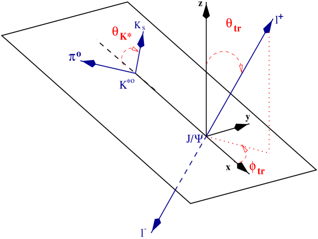
Figure 13: Definitions of the transversity angles $\theta_{tr}$, $\phi_{tr}$, and $\theta_{K^{*}}$. The angles $\theta_{tr}$ and $\phi_{tr}$ are determined in the $J/\psi$ rest frame. The angle $\theta_{K^{*}}$ is determined in the $K^{*}$ rest frame.

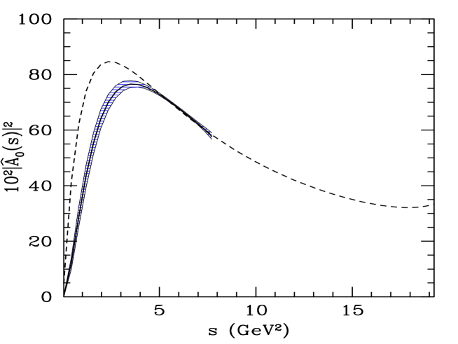
Figure 14: The helicity amplitude $|\hat{\cal A}_{0}(s)|^{2}$ in $B\to K^{*}\ell^{+}\ell^{-}$ at next-to-leading order (center line) and leading order (dashed). The band for NLO reflects theoretical uncertainties from input parameters.

Experimental results are conventionally expressed in terms of the spin amplitudes $\hat{\cal A}_{0,\bot,\|}$ normalized to unity, with $|\hat{\cal A}_{0}|^{2}+|\hat{\cal A}_{\bot}|^{2}+|\hat{\cal A}_{\|}|^{2}=1$. We show the polarization fractions, $\Gamma_{0}/\Gamma=|\hat{\cal A}_{0}(s)|^{2}$, $\Gamma_{\parallel}/\Gamma=|\hat{\cal A}_{\parallel}(s)|^{2}$ and $\Gamma_{\perp}/\Gamma=|\hat{\cal A}_{\perp}(s)|^{2}$ in the leading and next-to-leading order for the decay $B\to K^{*}\ell^{+}\ell^{-}$ in Figs (14), (15) and (16), respectively. Since the interference terms in the angular distribution are limited to Re(${\cal A}_{||}{\cal A}_{0}^{*}$), Im(${\cal A}_{\perp}{\cal A}_{0}^{*}$) and Im(${\cal A}_{\perp}{\cal A}_{||}^{*}$), there exists a phase ambiguity:

$$\phi_{||} \to -\phi_{||}~{},$$ (56)

$$\phi_{\perp} \to \pm\pi-\phi_{\perp}~{},$$ (57)

$$\phi_{\perp}-\phi_{||} \to \pm\pi-(\phi_{\perp}-\phi_{||})~{}.$$ (58)

To avoid this, we have plotted in Figs. (17) and (18) the functions $\cos\phi_{\parallel}(s)$, $\sin\phi_{\parallel}(s)$, and $\cos\phi_{\perp}(s)$, $\sin\phi_{\perp}(s)$, respectively, showing their behaviour at the leading and next-to-leading order. The dashed lines in these figures correspond to using the LO amplitudes, calculated in the LEET approach. In this order, the bulk of the parametric uncertainty resulting from the form factors cancels. Although, strictly speaking, the domain of validity of the LEET-based distributions is limited by the requirement of large energy of the $K^{*}$ (which we have translated into approximately $s<8\ GeV^{2}$), we show this distribution for the entire $s$-region allowed kinematically in $B\to K^{*}\ell^{+}\ell^{-}$. The shaded curves correspond to using the NLO contributions in the LEET approach. We compare the resulting amplitudes $|\hat{\cal A}_{0}|^{2}$, $|\hat{\cal A}_{\perp}|^{2}$, $|\hat{\cal A}_{\parallel}|^{2}$, $\phi_{\parallel}(s)$, and $\phi_{\perp}(s)$ at the value $s=m_{J/\psi}^{2}$ with the corresponding results from the four experiments in Table 4. In comparing these results for the phases, we had to make a choice between the two phase conventions shown in Eq. (58) and the phases shown in the last row of this table correspond to adopting the lower signs in these equations. We note that the short-distance amplitudes from the decay $B\to K^{*}\ell^{+}\ell^{-}$ are similar to their resonant counterparts measured in the decay $B\to J/\psi K^{*}$. We also note that a helicity analysis of the decay $B\to J/\psi K^{*}$ has been performed in the QCD factorization approach by Cheng et al. [47].

The structures in the phases shown in Fig. (17) and Fig.(18) deserve a closer look. We note that at the leading order, the phases $\phi_{\perp}(s)$ and $\phi_{\parallel}(s)$ are given by the following expressions:

$$\phi_{\perp}(s) = \textrm{Arg}\Big{[}{i\,\sqrt{\lambda}\over m_{b}\,m_{B}\,\sqrt{s}}\Big{\{}s\,{C_{9}}^{\rm eff}+2\,m_{b}\,m_{B}\,{C_{7}}^{\rm eff}\Big{\}}\,\xi_{\perp}(s)\Big{]}-\textrm{Arg}[{\cal A}_{0}(s)]~{},$$ (59)

$$\phi_{||}(s) = \textrm{Arg}\Big{[}{-i\,E_{V}\,\xi_{\perp}(s)\over m_{b}\,\sqrt{s}}\Big{\{}\Big{(}s\,{C_{9}}^{\rm eff}+2\,m_{b}\,m_{B}\,{C_{7}}^{\rm eff}\Big{)}-2\,m_{b}\,m_{B}\,\Big{(}{C_{7}}^{\rm eff}+{s\over 2\,m_{b}\,m_{B}}Y(s)\Big{)}({m_{V}^{2}\over m_{B}^{2}})\Big{\}}\Big{]}$$ (60)

$$-\textrm{Arg}[{\cal A}_{0}(s)],$$

where we can neglect the term proportional to $(m_{V}^{2}/m_{B}^{2})$ in the latter equation. The phase $\phi_{0}(s)\equiv\textrm{Arg}[{\cal A}_{0}(s)]$ is constant in the entire phase space, as shown in Fig. (19). The functions in the square brackets in Eqs. (59) and (60) are purely imaginary. However, due to the fact that in the SM the coefficients $C_{9}^{\rm eff}$ and $C_{7}^{\rm eff}$ have opposite signs, these phases become zero at a definite value of $s$, beyond which they change sign, yielding a step-function behaviour, shown by the dotted curves in the functions $\cos\phi_{\parallel}(s)$ and $\cos\phi_{\perp}(s)$ in Fig. (17) and Fig. (18), respectively. The position of the zero of the two functions, denoted, respectively, by $s^{\perp}_{0}$ and $s^{||}_{0}$, are given by solving the following equations:

$$\textrm{Arg}\Big{[}{i\,\sqrt{\lambda}\over m_{b}\,m_{B}\,\sqrt{s^{\perp}_{0}}}\Big{\{}s^{\perp}_{0}\,{C_{9}}^{\rm eff}(s^{\perp}_{0})+2\,m_{b}\,m_{B}\,{C_{7}}^{\rm eff}\Big{\}}\,\xi_{\perp}(s^{\perp}_{0})\Big{]} = \phi_{0}(s^{\perp}_{0})~{},$$ (61)

$$\textrm{Arg}\Big{[}{-i\,E_{V}\ \over m_{b}\,\sqrt{s^{||}_{0}}}\Big{\{}s^{||}_{0}\,{C_{9}}^{\rm eff}(s^{||}_{0})+2\,m_{b}\,m_{B}\,{C_{7}}^{\rm eff}\Big{\}}\,\xi_{\perp}(s^{||}_{0})\Big{]} = \phi_{0}(s^{||}_{0}).$$ (62)

For the assumed values of the Wislon coefficients and other parameters, the zeroes of the two functions, namely $s^{||}_{0}$ and $s^{\perp}_{0}$, occur at around $s\simeq 3$ GeV², in the lowest order, as can be seen in Figs. (17) and (18), respectively. The LO contributions in $\sin\phi_{\parallel}(s)$ and $\sin\phi_{\perp}(s)$ are constant, with a value around 0, with a small structure around $s\simeq 3\,GeV^{2}$, reflecting the sign flip of the imaginary part in ${\cal A}_{||}(s)$ (${\cal A}_{\perp}(s)$). At the NLO, the phases are influenced by the explicit $O(\alpha_{s})$ contributions from the factorizable and non-factorizable QCD corrections (see section 3), which also bring in parametric uncertainties with them. The most important effect is that the zeroes of the phases as shown for $\cos\phi_{\perp}(s)$ and $\cos\phi_{\parallel}(s)$ are shifted to the right, and the step-function type bahaviour of these phases in the LO gets a non-trivial shape. Note that in both figures a shoulder around $s\simeq 8\,GeV^{2}$ reflects charm production whose threshold lies at $s=4\,m_{c}^{2}$.

Group	$|\hat{\cal A}_{0}|^{2}$	$|\hat{\cal A}_{\perp}|^{2}$	$|\hat{\cal A}_{||}|^{2}$	$\phi_{\perp}$	$\phi_{\parallel}$
CLEO[33]	$0.52\pm 0.08$	$0.16\pm 0.09$	$0.32\pm 0.12$	$-3.03\pm 0.46$	$-3.00\pm 0.37$
CDF[34]	$0.59\pm 0.06$	$0.13^{+0.13}_{-0.11}$	$0.28\pm 0.12$	$-2.58\pm 0.54$	$-2.20\pm 0.47$
BaBar[35]	$0.60\pm 0.04$	$0.16\pm 0.03$	$0.24\pm 0.04$	$-2.97\pm 0.17$	$-2.50\pm 0.22$
Belle [36]	$0.60\pm 0.05$	$0.19\pm 0.06$	$0.21\pm 0.08$	$-3.15\pm 0.21$	$-2.86\pm 0.25$
This Work	$0.51$	$0.21$	$0.28$	$-3.25$	$-3.04$

Table 4: Current measurements of the decay amplitudes in the transversity basis for the decay $B\rightarrow J/\psi K^{*}$ . The corresponding amplitudes for the non-resonant decay $B\to K^{*}\ell^{+}\ell^{-}$ worked out in this paper in the LO approximation at $m_{\ell^{+}\ell^{-}}^{2}=m_{J/\psi}^{2}$ are given in the last row.

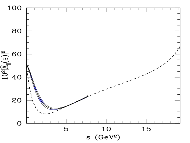
Figure 15: The helicity amplitude $|\hat{\cal A}_{\parallel}(s)|^{2}$ in $B\to K^{*}\ell^{+}\ell^{-}$ at next-to-leading order (solid center line) and leading order (dashed). The band for NLO reflects the theoretical uncertainties from the input parameters.

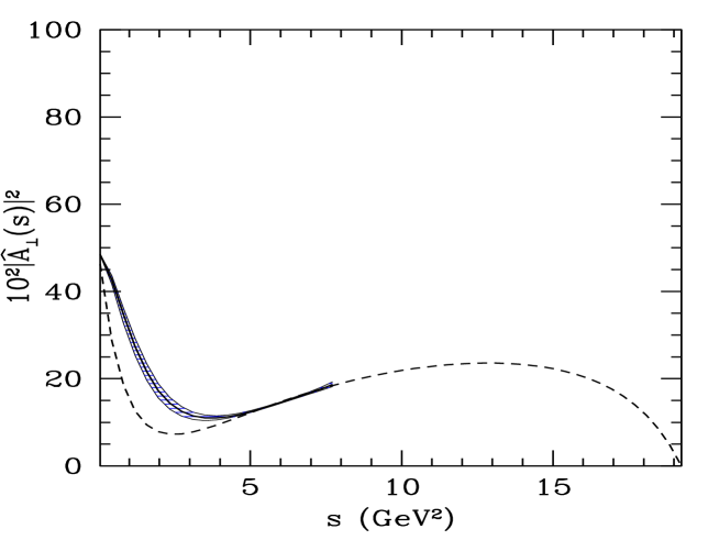
Figure 16: The helicity amplitude $|\hat{\cal A}_{\perp}(s)|^{2}$ in $B\to K^{*}\ell^{+}\ell^{-}$ at next-to-leading order (solid center line) and leading order (dashed). The band for NLO reflects theoretical uncertainties from input parameters.

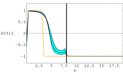
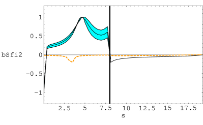
Figure 17: The functions $\cos\phi_{||}(s)$ and $\sin\phi_{||}(s)$ at next-to-leading order (solid center line) and leading order (dashed). The band reflects all theoretical uncertainties from parameters with most of the uncertainty due to the form factors $\xi_{i}(0)$. The vertical line at s = 8 $GeV^{2}$ represents the domain of validity of the LEET approach in our case.

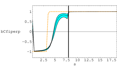
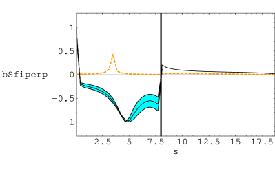
Figure 18: The functions $\cos\phi_{\perp}(s)$ and $\sin\phi_{\perp}(s)$ at next-to-leading order (solid center line) and leading order (dashed). The band reflects all theoretical uncertainties from parameters with most of the uncertainty due to the form factors $\xi_{i}(0)$.The vertical line at s = 8 $GeV^{2}$ represents the domain of validity of the LEET approach in our case.

\psfrag{s}{\hskip 8.5359pt$s\ (GeV^{2})$}\psfrag{b}{\hskip-28.45274pt$\phi_{0}(s)$}\includegraphics[width=227.62204pt,height=170.71652pt]{arg-A0.eps}

Figure 19: The phase $\phi_{0}(s)$ at next-to-leading order (solid center line) and leading order (dashed).

6 Decay Distributions in $B\rightarrow\rho\ell\bar{\nu_{\ell}}$

The differential decay rate for $B\rightarrow\rho(\rightarrow\pi^{+}\pi^{-})\ell\bar{\nu_{\ell}}$ can be expressed as follows [48, 49, 50]:

$${d^{4}\Gamma\over ds\ d\cos\theta_{\rho}\ d\cos\theta_{+}\ d\phi} = {3\over 8(4\pi)^{4}}G_{F}^{2}|V_{ub}|^{2}{\sqrt{\lambda}s\over m_{B}^{3}}{\it{{\cal B}(\rho\rightarrow\pi^{+}\pi^{-})}}$$ (63)

$$\Big{\{}(1-\ \cos\theta_{+})^{2}\sin^{2}\theta_{\rho}\ |H_{+}(s)|^{2}$$

$$+(1+\ \cos\theta_{+})^{2}\sin^{2}\theta_{\rho}\ |H_{-}(s)|^{2}$$

$$+4\ \sin^{2}\theta_{+}\ \cos^{2}\theta_{\rho}\ |H_{0}(s)|^{2}$$

$$-4\ \ \sin\theta_{+}\ (1-\cos\theta_{+})\ \sin\theta_{\rho}\ \cos\theta_{\rho}\ \cos\phi\ H_{+}(s)H_{0}(s)$$

$$+4\ \ \sin\theta_{+}\ (1+\cos\theta_{+})\ \sin\theta_{\rho}\ \cos\theta_{\rho}\ \cos\phi\ H_{-}(s)H_{0}(s)$$

$$-2\ \sin^{2}\theta_{+}\ \sin^{2}\theta_{\rho}\ \cos 2\phi\ H_{+}(s)H_{-}(s)\Big{\}}~{}.$$

The three angles $\theta_{+}$, $\theta_{\rho}$ and $\phi$ are defined as follows: $\theta_{+}$ is defined by the direction between the charged lepton and the recoiling vector meson measured in the $W$ rest frame, the polar angle $\theta_{\rho}$ is defined by the directions of the $\pi^{+}$ (or $\pi^{-}$) and the vector meson in the parent meson’s rest frame, and the azimuthal angle $\phi$ is the angle between the two planes, defined by the momenta of $\pi^{+}\pi^{-}$ and the lepton pair $\ell\bar{\nu}$.

The helicity amplitudes can in turn be related to the two axial-vector form factors, $A_{1}(s)$ and $A_{2}(s)$, and the vector form factor, $V(s)$, which appear in the hadronic current [50]:

$$H_{\pm}(s) = (m_{B}+m_{\rho})\ A_{1}(s)\mp 2\ {\sqrt{\lambda}\over m_{B}+m_{\rho}}\ V(s)~{},$$ (64)

$$H_{0}(s) = {1\over 2m_{\rho}\sqrt{s}}\ \Big{[}(m_{B}^{2}-m_{\rho}^{2}-s)(m_{B}+m_{\rho})\ A_{1}(s)-4\ {\lambda\over m_{B}+m_{\rho}}\ A_{2}(s)\Big{]}~{}.$$ (65)

Using Eqs.(17),(18) and (19) in Eqs. (65) and (64), we obtain the helicity amplitudes in the large energy Limit:

$$H_{\pm}(s) = 2\left[E_{\rho}\mp{\sqrt{\lambda}\over m_{B}}\right]\ \xi_{\perp}(s)~{},$$ (66)

$$H_{0}(s) = {1\over m_{B}\ m_{\rho}\ \sqrt{s}}\Big{[}m_{B}\ E_{\rho}\ (m_{B}^{2}-m_{\rho}^{2}-s)-2\ \lambda\Big{]}\ \xi_{\perp}(s)$$

$$+{2\ \lambda\over m_{B}E_{\rho}\sqrt{s}}\ \xi_{||}(s)~{}.$$

We give below the double differential decay rate (Dalitz distribution) for $B\rightarrow\rho(\rightarrow\pi^{+}\pi^{-})\ell\bar{\nu}$ in the variables $(s,\phi)$, $(s,\cos\theta_{+})$ and $(s,\cos\theta_{\rho})$, giving also the expressions for the individual contributions from the Helicity-$0$ and Helicity-$-1$ amplitudes for the Dalitz distribution in $(s,\cos\theta_{+})$:

$${d^{2}{\cal B}\over d\phi\ ds} = \tau_{B}{G_{F}^{2}\ s\ \sqrt{\lambda}\over 192m_{B}^{3}\pi^{4}}|V_{ub}|^{2}({\it{{\cal B}(\rho\rightarrow\pi^{+}\pi^{-})}})~{},$$

$$\Big{\{}|H_{0}(s)|^{2}+|H_{-}(s)|^{2}+|H_{+}(s)|^{2}-\cos 2\phi\ H_{-}(s)\ H_{+}(s)\Big{\}}~{},$$

$${d^{2}{\cal B}_{|H_{-}|^{2}}\over d\cos\theta_{+}\ ds} = \tau_{B}{G_{F}^{2}\ s\ \sqrt{\lambda}\over 256m_{B}^{3}\pi^{3}}|V_{ub}|^{2}({\it{{\cal B}(\rho\rightarrow\pi^{+}\pi^{-})}})\Big{\{}(1+\cos\theta_{+})^{2}\ |H_{-}(s)|^{2}\Big{\}}~{},$$

$${d^{2}{\cal B}_{|H_{0}|^{2}}\over d\cos\theta_{+}\ ds} = \tau_{B}{G_{F}^{2}\ s\ \sqrt{\lambda}\over 256m_{B}^{3}\pi^{3}}|V_{ub}|^{2}({\it{{\cal B}(\rho\rightarrow\pi^{+}\pi^{-})}})\Big{\{}2\ \sin^{2}\theta_{+}\ |H_{0}(s)|^{2}\Big{\}}~{},$$

$${d^{2}{\cal B}\over d\cos\theta_{+}\ ds} = \tau_{B}{G_{F}^{2}\ s\ \sqrt{\lambda}\over 256m_{B}^{3}\pi^{3}}|V_{ub}|^{2}({\it{{\cal B}(\rho\rightarrow\pi^{+}\pi^{-})}})~{},$$ (69)

$$\Big{\{}2\ \sin^{2}\theta_{+}\ |H_{0}(s)|^{2}+(1-\ \cos\theta_{+})^{2}\ |H_{+}(s)|^{2}+(1+\cos\theta_{+})^{2}\ |H_{-}(s)|^{2}\Big{\}}$$

$$= {d^{2}{\cal B}_{|H_{0}|^{2}}\over d\cos\theta_{+}\ ds}+{d^{2}{\cal B}_{|H_{+}|^{2}}\over d\cos\theta_{+}\ ds}+{d^{2}{\cal B}_{|H_{-}|^{2}}\over d\cos\theta_{+}\ ds}~{},$$

$${d^{2}{\cal B}\over d\cos\theta_{\rho}\ ds} = \tau_{B}{G_{F}^{2}\ s\ \sqrt{\lambda}\over 128m_{B}^{3}\pi^{3}}|V_{ub}|^{2}({\it{{\cal B}(\rho\rightarrow\pi^{+}\pi^{-})}})$$

$$\Big{\{}2\ \cos^{2}\theta_{\rho}\ |H_{0}(s)|^{2}+\ \sin^{2}\theta_{\rho}\ \Big{(}|H_{+}(s)|^{2}+|H_{-}(s)|^{2}\Big{)}\Big{\}}~{}.$$

In Figs. (21), (21), (22) and (23), we show, respectively, the Dalitz distributions ($d^{2}{\cal B}_{|H_{-}|^{2}}/d\cos\theta_{+}\ ds$), ($d^{2}{\cal B}_{|H_{0}|^{2}}/d\cos\theta_{+}\ ds$), ($d^{2}{\cal B}/d\cos\theta_{+}\ ds$) and ($d^{2}{\cal B}/d\cos\theta_{\rho}\ ds$).

Integrating out the angle $\theta_{+}$, $\theta_{\rho}$ and $\phi$ from Eq. (63), we obtain the total branching decay rate:

$${d{\cal B}\over ds} = \tau_{B}{G_{F}^{2}\ s\ \sqrt{\lambda}\over 96m_{B}^{3}\pi^{4}}|V_{ub}|^{2}({\it{{\cal B}(\rho\rightarrow\pi^{+}\pi^{-})}})\Big{\{}|H_{0}(s)|^{2}+|H_{+}(s)|^{2}+|H_{-}(s)|^{2}\Big{\}}$$

$$= {d{\cal B}_{|H_{0}|^{2}}\over ds}+{d{\cal B}_{|H_{+}|^{2}}\over ds}+{d{\cal B}_{|H_{-}|^{2}}\over ds}~{}.$$

Just as in the decay $B\to K^{*}\ell^{+}\ell^{-}$, the contribution from the $|H_{+}(s)|^{2}$ is negligible, and we do not show it here. The contributions from the $|H_{-}(s)|^{2}$, $|H_{0}(s)|^{2}$ and the total are shown in Figs. (24), (25) and (26), respectively. The impact of the NLO correction on the various branching ratios in $B\rightarrow\rho\ell\nu_{\ell}$ is less significant than in the $B\rightarrow K^{*}\ell^{+}\ell^{-}$ decay, reflecting the absence of the penguin-based amplitudes in the former decay.

Concerning the $B\rightarrow\rho\ell\nu_{\ell}$ form factors, one has to consider the SU(3)-breaking effects in relating them to the corresponding form factors in $B\to K^{*}\ell^{+}\ell^{-}$. For the form factors in full QCD, they have been evaluated within the Light-cone QCD sum-rule approach [51, 19, 52], Lattice-QCD [17], and in quark models of the more recent vintage [54, 53]. Based on the Light-cone QCD sum-rule approach, we estimate the SU(3)-breaking in the ratio of the LEET-based form factors at $s=0$ as

$$\zeta_{SU(3)}={\xi^{(K^{*})}_{\perp,||}(0)\over\xi^{(\rho)}_{\perp,||}(0)}=1.3\pm 0.06~{}.$$ (72)

With this and $\xi^{(K^{*})}_{\perp}(0)$ from Table 3, we obtain:

$$\xi^{(\rho)}_{\perp}(0)=0.22\pm 0.04~{}.$$ (73)

The results for the various helicity amplitudes $H_{+}(0)$, $H_{-}(0)$, $\sqrt{s}H_{0}(0)$, and the ratio $H_{-}(0)/H_{+}(0)$ in the decay $B\to\rho\ell\nu_{\ell}$ are given in Table 5, and compared with some other estimates of the same in the literature. We recall that in our approach both $\xi^{(K^{*})}_{\perp}(0)$ and $\xi^{(\rho)}_{\perp}(0)$ are smaller due to the normalization of the former from data on $B\to K^{*}\gamma$ decay rate. This is reflected in the smaller values of the helicity amplitudes in this work compared to the other approaches.

To get the $B\rightarrow\rho\ \ell\ \nu_{\ell}$ form factors at $s\neq 0$, we use the same parametrization as the one for the $B\rightarrow K^{*}\ell^{+}\ell^{-}$ form factors:

$$\xi^{(\rho)}_{\perp,||}(s)={\xi^{(K^{*})}_{\perp,||}(s)\over\zeta_{SU(3)}}~{}.$$ (74)

This parametrization has been used in calculating the differential branching ratios shown for the restricted region $s\leq 7$ GeV² in Figs. (24), (25) and (26). While we do not insist on using our approach to cover the small $E_{\rho}$-region (and, hence higher values of $s$) in the decay $B\to\rho\ell\nu_{\ell}$, but for the sake of comparison with recent data and some existing estimates of the various helicity amplitudes in the literature, we use the $s$-dependence in (74) to estimate $H_{i}(s)$ in the entire kinematic region. Numerical results from our work are shown in the first row of Table 6 for $s=s_{\rm max}$. The equality $H_{+}(s_{\rm max})=H_{-}(s_{\rm max})=H_{0}(s_{\rm max})$ is imposed by the kinematics of the decay $B\to\rho\ell\nu_{\ell}$, but we note that our results are numerically smaller than the ones following from other form factor models shown in this table. This is again to be traced back to our normalization of the function $\xi_{\perp}^{K^{*}}(0)$ and (74). In Table 7, we present various reduced partial widths for $B\to\rho\ell\nu_{\ell}$ for the longitudinal part $\Gamma_{L}=\Gamma_{0}$, transverse part $\Gamma_{T}=\Gamma_{-}+\Gamma_{+}$, the total reduced width $\Gamma_{\rm Total}$, factoring out the CKM matrix element $|V_{ub}|^{2}$, and the ratio $\Gamma_{L}/\Gamma_{T}$, and compare them with the corresponding estimates in the literature. Our values for the total reduced decay widths are smaller than the other five shown in Table  7. For the form factor model in Ref. [53], we show a detailed comparison and note that our estimate of $\Gamma_{T}$ (derived from LEET and data) is significantly smaller than in this model, but our $\Gamma_{L}$, with input from the Light-cone QCD sum rules, is comparable to the one in Ref. [53]. This has the consequence that in our approach $\Gamma_{L}$ and $\Gamma_{T}$ are about equal, as opposed to theirs where $\Gamma_{L}$ is significantly smaller than $\Gamma_{T}$, which will be tested in future experiments.

Finally, we note that the smaller values of the form factors in the LEET-based approach used in this work lead to estimates of $|V_{ub}|$ from the measured exclusive decay rate for $B\to\rho\ell\nu_{\ell}$ [56], which are in agreement with the PDG 2004 average [57] $|V_{ub}|=(3.67\pm 0.47)\times 10^{-3}$. This can also be seen as follows: Using the central values of $|V_{ub}|$ and the lifetime $\tau_{B^{0}}=1.536$ ps from PDG 2004, and the reduced width in the LEET approach $\Gamma_{\rm Total}=10.49$ ps^-1 from Table 7, we get ${\cal B}(B\to\rho\ell\nu_{\ell})=2.18\times 10^{-4}$, in comfortable agreement with the measured branching ratio by the BABAR collaboration [56] ${\cal B}(B\to\rho\ell\nu_{\ell})=(2.14\pm 0.21\pm 0.48)\times 10^{-4}$. In contrast, the allowed range of $|V_{ub}|$ obtained recently by the BABAR collaboration [56] using the form factors from the Light-cone QCD sum-rules [52] is $|V_{ub}|=(2.82\pm 0.18\pm 0.30\pm 0.18)\times 10^{-3}$, with similar values for the quark-model based form factors [55]. This is significantly smaller than the PDG 2004 average [57] $|V_{ub}|=(3.67\pm 0.47)\times 10^{-3}$. Thus, it is evident that, unless the corrections to the LEET-based approach are very significant, data for the radiative decays $B\to(K^{*},\rho,\omega)\gamma$, but also for the semileptonic decay $B\to\rho\ell\nu_{\ell}$, favour smaller form factors than obtained in the QCD sum rule approaches or the quark models.

\psfrag{c}{\hskip 8.5359pt$s\ (GeV^{2})$}\psfrag{a}{\hskip-119.50148pt$d^{2}{\cal B}_{|H_{-}|^{2}}/ds\ d\cos\theta_{+}|V_{ub}|^{2}$}\psfrag{b}{$\cos\theta_{+}$}\includegraphics[width=341.43306pt,height=256.0748pt]{figr2.eps}

Figure 20: Partial Dalitz distribution ${d^{2}{\cal B}_{|H_{-}|^{2}}(B\rightarrow\rho\ell\bar{\nu_{\ell}})\over d\cos\theta_{+}\ ds}$.

\psfrag{c}{\hskip 8.5359pt$s\ (GeV^{2})$}\psfrag{a}{\hskip-119.50148pt$d^{2}{\cal B}_{|H_{-}|^{2}}/ds\ d\cos\theta_{+}|V_{ub}|^{2}$}\psfrag{b}{$\cos\theta_{+}$}\psfrag{c}{\hskip 8.5359pt$s\ (GeV^{2})$}\psfrag{a}{\hskip-99.58464pt$d^{2}{\cal B}_{|H_{0}|^{2}}/ds\ d\cos\theta_{+}|V_{ub}|^{2}$}\psfrag{b}{$\cos\theta_{+}$}\includegraphics[width=341.43306pt,height=256.0748pt]{figr3.eps}

Figure 21: Partial Dalitz distribution ${d^{2}{\cal B}_{|H_{0}|^{2}}(B\rightarrow\rho\ell\bar{\nu_{\ell}})\over d\cos\theta_{+}\ ds}$.

\psfrag{c}{\hskip 8.5359pt$s\ (GeV^{2})$}\psfrag{a}{\hskip-99.58464pt$d^{2}{\cal B}/ds\ d\cos\theta_{+}|V_{ub}|^{2}$}\psfrag{b}{$\cos\theta_{+}$}\includegraphics[width=341.43306pt,height=256.0748pt]{figr4.eps}

Figure 22: Dalitz distribution ${d^{2}{\cal B}(B\rightarrow\rho\ell\bar{\nu_{\ell}})\over{\rm d}\cos\theta_{+}\ ds}$ .

\psfrag{c}{\hskip 8.5359pt$s\ (GeV^{2})$}\psfrag{a}{\hskip-99.58464pt$d^{2}{\cal B}/ds\ d\cos\theta_{\rho}|V_{ub}|^{2}$}\psfrag{b}{$\cos\theta_{\rho}$}\includegraphics[width=341.43306pt,height=256.0748pt]{figr5.eps}

Figure 23: Dalitz distribution ${d^{2}{\cal B}(B\rightarrow\rho\ell\bar{\nu_{\ell}})\over\cos\theta_{\rho}\ ds}$.

\psfrag{a}{$s\ (GeV^{2})$}\psfrag{b}{\hskip-85.35826pt$d{\cal B}_{|H_{-}|^{2}}/ds\ |V_{ub}|^{2}$}\psfrag{c}{}\includegraphics[width=341.43306pt,height=256.0748pt]{figr6.eps}

Figure 24: The dilepton invariant mass distribution $d{\cal B}_{|H_{-}|^{2}}/ds$ for $B\rightarrow\rho\ell\bar{\nu}$ at next-to-leading order (solid center line) and leading order (dashed). The band reflects theoretical uncertainties from input parameters.

\psfrag{a}{\hskip-28.45274pt$s\ (GeV^{2})$}\psfrag{b}{\hskip-85.35826pt$d{\cal B}_{|H_{0}|^{2}}/ds\ |V_{ub}|^{2}$}\includegraphics[width=341.43306pt,height=256.0748pt]{figr8.eps}

Figure 25: The dilepton invariant mass distribution $d{\cal B}_{|H_{0}|^{2}}/ds$ for $B\rightarrow\rho\ell\bar{\nu}$ at next-to-leading order (solid center line) and leading order (dashed). The band reflects theoretical uncertainties from input parameters.

\psfrag{a}{$s\ (GeV^{2})$}\psfrag{b}{\hskip-71.13188pt$d{\cal B}/ds\ |V_{ub}|^{2}$}\psfrag{c}{}\includegraphics[width=341.43306pt,height=256.0748pt]{figr9.eps}

Figure 26: The dilepton invariant mass distribution for $B\rightarrow\rho\ell\bar{\nu}$ at next-to-leading order (solid center line) and leading order (dashed). The band reflects theoretical uncertainties from input parameters.

	$H_{+}\left(0\right)$	$H_{-}\left(0\right)$	$H_{-}\left(0\right)/H_{+}\left(0\right)$	$\sqrt{s}H_{0}\left(0\right)$
This Work	0.048	2.274	47.002	7.459
Ref.[53]	0.256	3.253	12.714	8.737
QM [54]	0.163	2.942	18.014	8.202
LCSR [19]	0.055	3.103	56.767	10.158
Lattice [17]	0.0898	4.224	47.020	10.914

Table 5: Various helicity amplitudes for $B\to\rho\ell\nu_{\ell}$ calculated at $s=0$, using different models.

	$H_{+}\left(s_{\max}\right)$	$H_{-}\left(s_{\max}\right)$	$H_{0}\left(s_{\max}\right)$	$\sqrt{s}H_{0}\left(s_{\max}\right)$
This Work	1.919	1.919	1.919	8.656
Ref.[53]	2.362	2.362	2.362	10.652
QM [54]	2.952	2.952	2.952	13.313
LCSR [19]	2.782	2.782	2.782	12.549
Lattice [17]	2.826	2.826	2.826	12.744

Table 6: Various helicity amplitudes for $B\to\rho\ell\nu_{\ell}$ calculated at $s=s_{\max}$, using different models.

	$\Gamma_{-}$	$\Gamma_{+}$	$\Gamma_{L}=\Gamma_{0}$	$\Gamma_{T}=\Gamma_{-}+\Gamma_{+}$	$\Gamma_{\mathrm{Total}}$	$\Gamma_{L}/\Gamma_{T}$
This Work	4.978	0.084	5.423	5.062	10.49	1.07
Ref.[53]	9.662	0.059	6.095	9.721	15.82	0.63
QM [54]	-	-	-	-	15.8$\pm$2.3	0.88$\pm 0.08$
LCSR [19]	-	-	-	-	13.5$\pm 4.0$	0.52$\pm$0.08
Lattice [17]	-	-	-	-	16.5${}_{-2.3}^{+3.5}$	0.80${}_{-0.03}^{+0.04}$
ISGW2 [55]	-	-	-	-	14.2	0.3

Table 7: Reduced partial and total decay rates for $B\to\rho\ell\nu_{\ell}$ in units of ps^-1, the ratio $\Gamma_{L}/\Gamma_{T}$, obtained in our approach, and using different models for form factors. To get the decay widths, one has to multiply the entries in this table with $|V_{ub}|^{2}$.

7 Determination of $|V_{ub}|/|V_{ts}|$ from $B\to\rho\ell\nu_{\ell}$ and
$B\to K^{*}\ell^{+}\ell^{-}$ Decays

The measurement of exclusive $B\rightarrow\rho\ell\bar{\nu}$ decays is one of the major goals of B physics. It provides a good tool for the extraction of $|V_{ub}|$, provided the form factors can be either measured precisely or calculated from first principles, such as the lattice-QCD framework. To reduce the non-perturbative uncertainty in the extraction of $V_{ub}$, we propose to study the ratios of the differential decay rates in $B\to\rho\ell\nu_{\ell}$ and $B\to K^{*}\ell^{+}\ell^{-}$ involving definite helicity states. These $s$-dependent ratios $R_{i}(s)$, $(i=0,-1,+1)$ are defined as follows:

$$R_{i}(s)={{d\Gamma_{H_{i}}^{B\rightarrow K^{*}\ l^{+}l^{-}}/ds}\over{d\Gamma_{H_{i}}^{B\rightarrow\rho\ l\bar{\nu}}/ds}}$$ (75)

The ratio $R_{-}(s)$ suggests itself as the most interesting one, as the form factor dependence essentially cancels (in the SU(3)-symmetry limit). From this, one can measure the ratio $|V_{ts}|/|V_{ub}|$. In Fig. (27), we plot $R_{-}(s)$ for three representative values of the CKM ratio $R_{b}=|V_{ub}|/|V_{tb}V_{ts}^{*}|=|V_{ub}|/|V_{cb}|=0.08$, $0.094$, and $0.11$. We also show the ratio $R_{0}(s)$, where the form factor dependence does not cancel. For the LEET form factors used here, the compounded theoretical uncertainty is shown by the shaded regions. This figure suggests that high statistics experiments may be able to determine the CKM-ratio from measuring $R_{-}(s)$ (and $R_{0}(s)$) at a competitive level compared to the other methods en vogue in experimental studies.

\psfrag{a}{ $s\ (GeV^{2})$}\psfrag{b}{\hskip-71.13188pt$R_{-}(s)/10^{-2}$}\includegraphics[width=455.24408pt,height=341.43306pt]{figsm7.eps}

Figure 27: The Ratio $R_{-}(s)$ with three indicated values of the CKM ratio $R_{b}\equiv|V_{ub}|/|V_{tb}V_{ts}^{*}|$. The bands reflect the theoretical uncertainty from $\zeta_{SU(3)}=1.3\pm 0.06$ and $\xi^{(K^{*})}_{{\perp}}(0)=0.28\pm 0.04$.

\psfrag{s}{ $\mathbf{s\ (GeV^{2})}$}\psfrag{R0}{\hskip-56.9055pt$\mathbf{R_{0}(s)\times 10^{-2}}$}\psfrag{Rb11}{$\mathbf{R_{b}=0.11}$}\psfrag{Rb94}{$\mathbf{R_{b}=0.094}$}\psfrag{Rb8}{$\mathbf{R_{b}=0.08}$}\includegraphics[width=455.24408pt,height=341.43306pt]{figsm9.eps}

Figure 28: The Ratio $R_{0}(s)$ with three indicated values of the CKM ratio $R_{b}\equiv|V_{ub}|/|V_{tb}V_{ts}^{*}|$. The bands reflect the theoretical uncertainty from $\zeta_{SU(3)}=1.3\pm 0.06$ and $\xi^{(K^{*})}_{{\perp}}(0)=0.28\pm 0.04$.

8 The Ratios $R_{-}(s)$ and $R_{0}(s)$ as Probes of New Physics in $B\rightarrow K^{*}\ l^{+}l^{-}$

In order to look for new physics in $B\rightarrow K^{*}\ell^{+}\ell^{-}$, we propose to study the ratios $R_{0}(s)$ and $R_{-}(s)$, introduced in the previous section. As well known, new physics can distort the dilepton invariant mass spectrum and the forward-backward asymmetry in a non-trivial way.

To illustrate generic SUSY effects in ${B\rightarrow K^{*}\ell^{+}\ell^{-}}$, we note that the Wilson coefficients $C^{\bf eff}_{7}$, $C^{\bf eff}_{8}$, $C_{9}$ and $C_{10}$ receive additional contributions from the supersymmetric particles. We incorporate these effects by assuming that the ratios of the Wilson coefficients in these theories and the SM deviate from 1. These ratios for $k=7,8,9,10$ are defined as follows:

$$r_{k}(\mu)={C_{k}^{SUSY}\over C_{k}^{SM}}~{}.$$ (76)

They depend on the renormalization scale (except for $C_{10}$), for which we take $\mu=m_{b,pole}$. For the sake of illustration, we use representative values for the large-$\tan\beta$ SUGRA model, in which the ratios $r_{7}$ and $r_{8}$ actually change their signs. The supersymmetric effects on the other two Wilson coefficients $C_{9}$ and $C_{10}$ are generally small in the SUGRA models, leaving $r_{9}$ and $r_{10}$ practically unchanged from their SM value. To be specific, we take

$$r_{7}=-1.2,\ \ r_{8}=-1,\ \ \ r_{9}=1.03,\ \ r_{10}=1.0~{}.$$ (77)

In Figs. (29) and (30), we present a comparative study of the SM and SUGRA partial distribution for $H_{-}$ and $H_{0}$, respectively. In doing this, we also show the attendant theoretical uncertainties for the SM, worked out in the LEET approach in this paper. For these distributions, we have used the form factors from [18] with the SU(3)-symmetry breaking parameter taken in the range $\zeta_{SU(3)}=1.3\pm 0.06$. Figs. (29) and (30) illustrate clearly that despite non-perturbative uncertainties, it is possible, in principle, in the low $s$ region to distinguish between the SM and a SUGRA-type models, provided the ratios $r_{k}$ differ sufficiently from 1.

\psfrag{a}{ $s\ (GeV^{2})$}\psfrag{b}{\hskip-71.13188pt$R_{-}(s)/10^{-2}$}\includegraphics[width=341.43306pt,height=256.0748pt]{figsm8.eps}

Figure 29: The Ratio $R_{-}(s)$ with $|V_{ub}|/|V_{tb}V_{ts}^{*}|=0.094$ in the Standard Model and in SUGRA, with $(r_{7},\ r_{8})=(-1.2,\ -1)$, $\zeta_{SU(3)}=1.3$ and $\xi^{(K^{*})}_{{\perp}}(0)=0.28$ represented, respectively, by the shaded area and the solid curve. The shaded area depicts the theoretical uncertainty $\zeta_{SU(3)}=1.3\pm 0.06$ and $\xi^{(K^{*})}_{{\perp}}(0)=0.28\pm 0.04$.

\psfrag{s}{ $\mathbf{s\ (GeV^{2})}$}\psfrag{R0}{\hskip-56.9055pt$\mathbf{R_{0}(s)\times 10^{-2}}$}\psfrag{Rb94}{$\mathbf{R_{b}=0.094}$}\includegraphics[width=341.43306pt,height=256.0748pt]{figsm10.eps}

Figure 30: The Ratio $R_{0}(s)/$ with $|V_{ub}|/|V_{tb}V_{ts}^{*}|=0.094$ in the Standard Model and in SUGRA, with $(r_{7},\ r_{8})=(-1.2,\ -1)$, $\zeta_{SU(3)}=1.3$ and $\xi^{(K^{*})}_{{\perp}}(0)=0.28$ represented, respectively, by the shaded area and the solid curve. The shaded area depicts the theoretical uncertainty $\zeta_{SU(3)}=1.3\pm 0.06$ and $\xi^{(K^{*})}_{{\perp}}(0)=0.28\pm 0.04$.

9 Summary and Concluding Remarks

Summarizing briefly our results, we have reported an $O(\alpha_{s})$-improved analysis of the various helicity components in the decays $B\to K^{*}\ell^{+}\ell^{-}$ and $B\to\rho\ell\nu_{\ell}$, carried out in the context of the Large-Energy-Effective-Theory. The underlying symmetries in the large energy limit lead to an enormous simplification as they reduce the number of independent form factors in these decays. The LEET-symmetries are broken by QCD corrections, and we have calculated the helicity components implementing the $O(\alpha_{s})$ corrections. The results presented here make use of the form factors calculated in the QCD sum rule approach. The LEET form factor $\xi_{\perp}^{K^{*}}(0)$ is constrained by current data on $B\to K^{*}\gamma$. As the theoretical analysis is restricted to the lower part of the dilepton invariant mass region in $B\to K^{*}\ell^{+}\ell^{-}$, typically $s<8$ GeV², errors in this form factor are not expected to severely limit theoretical precision. This implies that distributions involving the $H_{-}(s)$ helicity component can be calculated reliably. Precise measurements of the two LEET form factors $\xi_{\perp}^{\rho}(s)$ and $\xi_{\parallel}^{\rho}(s)$ in the decays $B\to\rho\ell\nu_{\ell}$ can be used to largely reduce the residual model dependence. With the assumed form factors, we have worked out a number of single and double (Dalitz) distributions in $B\to\rho\ell\nu_{\ell}$, which need to be confronted with data. An analysis of the decays $B\to K^{*}\ell^{+}\ell^{-}$ is also carried out in the so-called transversity basis. We have compared the LEET-based amplitudes in this basis with the data currently available on $B\to K^{*}J/\psi(\to\ell^{+}\ell^{-})$ and find that the short-distance based transversity amplitudes are very similar to their long-distance counterparts. We also show the $O(\alpha_{s})$ effects on the forward-backward asymmetry, confirming essentially the earlier work of Beneke, Feldmann and Seidel [13]. Combining the analysis of the decay modes $B\to K^{*}\ell^{+}\ell^{-}$ and $B\to\rho\ell\nu_{\ell}$, we show that the ratios of differential decay rates involving definite helicity states, $R_{-}(s)$ and $R_{0}(s)$, can be used for testing the SM precisely. We work out the dependence of these ratios on the CKM matrix elements $|V_{ub}|/|V_{ts}|$. We have also analyzed possible effects on these ratios from New Physics contributions, exemplified by representative values for the effective Wilson coefficients in the large-$\tan\beta$ SUGRA models. The main thrust of this paper lies, however, on showing that the currently prevailing theoretical uncertainties on the SM distributions in $B\to K^{*}\ell^{+}\ell^{-}$ can be largely reduced by using the LEET approach and data on $B\to K^{*}\gamma$ and $B\to\rho\ell\nu_{\ell}$ decays. Finally, we remark that the current experimental limits on $B\to(X_{s},K^{*})\ell^{+}\ell^{-}$ decays (and the observed $B\to K\ell^{+}\ell^{-}$ decay) [39, 40, 41, 42] are already probing the SM-sensitivity. With the integrated luminosities over the next couple of years at the $B$ factories, the helicity analysis in $B\to\rho\ell\nu_{\ell}$ and $B\to K^{*}\ell^{+}\ell^{-}$ decays presented here can be carried out experimentally.

References

• [1] See, e.g., C. Greub, talk given at the 8th International Symposium on Heavy Flavour Physics, Southampton, England, 25-29 Jul 1999. [hep-ph/9911348].
• [2] M. S. Alam et al. [CLEO Collaboration], Phys. Rev. Lett.  74 (1995) 2885.
• [3] S. Chen et al. [CLEO Collaboration], Phys. Rev. Lett., 87 (2001) 251807 [hep-ex/0108032].
• [4] R. Barate et al. [ALEPH Collaboration], Phys. Lett. B429, (1998) 169.
• [5] K. Abe et al. [BELLE Collaboration], Phys. Lett.  B511 (2001) 151 [hep-ex/0103042].
• [6] K. Chetyrkin, M. Misiak and M. Münz, Phys. Lett. B400 (1997) 206; E: B425 (1998) 414 [hep-ph/9612313].
• [7] A. L. Kagan and M. Neubert, Eur. Phys. J. C7, 5 (1999) [hep-ph/9805303].
• [8] P. Gambino and M. Misiak, Nucl. Phys.  B611 (2001) 338 [hep-ph/0104034].
• [9] A. Ali, E. Lunghi, C. Greub and G. Hiller, DESY 01-217 [hep-ph/0112300].
• [10] H. Tajima [BELLE Collaboration], Plenary Talk, XX International Symposium on Lepton and Photon Interactions at High Energies, July 23 - 28, 2001, Rome.
• [11] B. Aubert et al. [BABAR Collaboration] Phys. Rev. Lett.  88 (2002) 101805 [hep-ex/0110065].
• [12] A. Ali and A. Y. Parkhomenko, Eur. Phys. J. C23 (2002) 89 [hep-ph/0105302].
• [13] M. Beneke, T. Feldmann and D. Seidel Nucl. Phys. B612 (2001) 25 [hep-ph/0106067].
• [14] S. W. Bosch and G. Buchalla, Nucl. Phys. B621 (2002) 459 [hep-ph/0106081].
• [15] M. J. Dugan and B. Grinstein, Phys. Lett. B255, 583 (1991).
• [16] J. Charles, A. Le Yaouanc, L. Oliver, O. Pene and J. C. Raynal, Phys. Rev.  D60 (1999) 014001 [hep-ph/9812358].
• [17] L. Del Debbio, J. M. Flynn, L. Lellouch and J. Nieves [UKQCD Collaboration], Phys. Lett. B416 (1998) 392 [hep-lat/9708008].
• [18] A. Ali, P. Ball, L. T. Handoko and G. Hiller, Phys. Rev. D 61 (2000) 074024 [hep-ph/9910221].
• [19] P. Ball and V. M. Braun, Phys. Rev. D58 (1998) 094016 [hep-ph/9805422].
• [20] A. Soni, Nucl. Phys. Proc. Suppl.  47 (1996), 43 [hep-lat/9510036].
• [21] M. Beneke, G. Buchalla, M. Neubert and C. T. Sachrajda, Phys. Rev. Lett.  83 (1999) 1914 [hep-ph/9905312].
• [22] A. L. Kagan and M. Neubert, Report CLNS-01-1756 hep-ph/0110078.
• [23] M. Beneke and T. Feldmann, Nucl. Phys. B592 (2001) 3 [hep-ph/0008255].
• [24] D. Melikhov, N. Nikitin and S. Simula, Phys. Lett. B 442 (1998) 381 [hep-ph/9807464].
• [25] T. M. Aliev, C. S. Kim and Y. G. Kim, Phys. Rev. D 62 (2000) 014026 [hep-ph/9910501].
• [26] C. S. Kim, Y. G. Kim, C. D. Lu and T. Morozumi, Phys. Rev. D62 (2000) 034013 [hep-ph/0001151].
• [27] C. S. Kim, Y. G. Kim and C. D. Lu, Phys. Rev. D64 (2001) 094014 [hep-ph/0102168].
• [28] X. S. Nguyen and X. Y. Pham, hep-ph/0110284.
• [29] C. H. Chen and C. Q. Geng, hep-ph/0203003.
• [30] I. Dunietz et al., Phys. Rev. D43, 2193 (1991).
• [31] G. Kramer and W. F. Palmer, Phys. Rev. D 45 (1992) 193.
• [32] A.S. Dighe, I. Dunietz, H.J. Lipkin and J.L. Rosner, Phys. Lett. B369 (1996) 144 [hep-ph/9511363].
• [33] C.P. Jessop et al. (CLEO Collaboration), Phys. Rev. Lett. 79, (1997) 4533 [hep-ex/9702013].
• [34] T. Affolder et al. (CDF Collaboration), Phys. Rev. Lett. 85, 4668 (2000) [hep-ex/0007034].
• [35] B. Aubert et al. (BABAR Collaboration), Phys. Rev. Lett. 87 (2001) 241801; BABAR-CONF-02/01 [hep-ex/0203007].
• [36] K. Abe et al. (BELLE Collaboration), KEK Preprint 2002-17 [hep-ex/0205021].
• [37] F. Krüger, L. M. Sehgal, N. Sinha and R. Sinha, Phys. Rev. D 61 (2000) 114028; [Erratum-ibid. D 63 (2001) 019901] [hep-ph/9907386].
• [38] N. Cabibbo, Phys. Rev. Lett. 10, 531 (1963),
M. Kobayashi and T. Maskawa, Prog. Theor. Phys. 49, 652 (1973).
• [39] K. Abe et al. [Belle Collaboration], BELLE-CONF-0110 [hep-ex/0107072];
K. Abe et al. [BELLE Collaboration], Phys. Rev. Lett. 88 (2002) 021801 [hep-ph/0109026].
• [40] B. Aubert et al. [BABAR Collaboration], BABAR-CONF-01/24, SLAC-PUB-8910 [hep-ex/0107026].
• [41] T. Affolder et al. [CDF Collaboration], Phys. Rev. Lett.  83 (1999) 3378 [hep-ex/9905004].
• [42] S. Anderson et al. [CLEO Collaboration], Phys. Rev. Lett.  87 (2001) 181803 [hep-ex/0106060].
• [43] B. Grinstein, M. J. Savage and M. B. Wise, Nucl. Phys. B319 (1989) 271.
• [44] G. Buchalla, A. J. Buras and M. E. Lautenbacher, Rev. Mod. Phys. 68 (1996) 1125 [hep-ph/9512380].
• [45] H. H. Asatrian, H. M. Asatrian, C. Greub and M. Walker, Phys. Lett.  B507 (2001) 162 [hep-ph/0103087]; Phys. Rev.  D65 (2002) 074004 [hep-ph/0109140].
• [46] A. Ali, T. Mannel and T. Morozumi, Phys. Lett. B273 (1991) 505.
• [47] H. Y. Cheng, Y. Y. Keum and K. C. Yang, Phys. Rev. D 65 (2002) 094023 [hep-ph/0111094].
• [48] J. G. Körner and G. A. Schuler, Z. Phys. C 46 (1990) 93.
• [49] J. G. Körner and G. A. Schuler, Phys. Lett. B 226 (1989) 185.
• [50] J. D. Richman and P. R. Burchat, Rev. Mod. Phys.  67 (1995) 893 [hep-ph/9508250].
• [51] A. Ali, V. M. Braun and H. Simma, Z. Phys.  C63 (1994) 437 [hep-ph/9401277].
• [52] For a theoretically improved calculation of $B\to$ light vector meson form factors in the Light-cone QCD sum-rule approach, see P. Ball and R. Zwicky, Phys. Rev. D 71 (2005) 014029 [hep-ph/0412079].
• [53] A. H. S. Gilani, Riazuddin and T. A. Al-Aithan, JHEP 0309 (2003) 065 [hep-ph/0304183].
• [54] M. Beyer and D. Melikhov, Phys. Lett. B 436 (1998) 344 [hep-ph/9807223].
• [55] N. Isgur, D. Scora, B. Grinstein, and M.B. Wise, Phys. Rev. D 39, 799 (1989); D. Scora, and N. Isgur, Phys. Rev. D 52, 2783 (1995) [hep-ph/9503486]
• [56] B. Aubert et al. [BABAR Collaboration], [hep-ex/0507003].
• [57] S. Eidelman et al. [Particle Data Group], Phys. Lett. B 592, 1 (2004).