Phenomenology of A Three-Family Standard-like String Model

Abstract

We discuss the phenomenology of a three-family supersymmetric Standard-like Model derived from the orientifold construction, in which the ordinary chiral states are localized at the intersection of branes at angles. In addition to the Standard Model group, there are two additional $U(1)^{\prime}$ symmetries, one of which has family non-universal and therefore flavor changing couplings, and a quasi-hidden non-abelian sector which becomes strongly coupled above the electroweak scale. The perturbative spectrum contains a fourth family of exotic ($SU(2)$- singlet) quarks and leptons, in which, however, the left-chiral states have unphysical electric charges. It is argued that these decouple from the low energy spectrum due to hidden sector charge confinement, and that anomaly matching requires the physical left-chiral states to be composites. The model has multiple Higgs doublets and additional exotic states. The moduli-dependent predictions for the gauge couplings are discussed. The strong coupling agrees with experiment for reasonable moduli, but the electroweak couplings are too small.

I Introduction

Despite an enormous amount of promise and interest in superstring/M theory, it is still difficult to construct models with a fully realistic effective low energy four-dimensional limit from first principles. The (related) difficulties include the fact that only certain limiting corners of M theory are perturbative, there are many possible compactifications of the extra dimensions, the cosmological constant, the method of supersymmetry breaking, the difficulty of constructing a realistic spectrum for the effective theory, and the stabilization of moduli. One direction, the subject of this paper, is to examine concrete semi-realistic constructions in as much detail as possible. One does not expect to find a fully realistic model. Rather, the goals are: (1) to develop calculational techniques, (2) to suggest promising directions for new constructions, and (3) to find examples of possible new physics at the TeV scale that might emerge from explicit top-down string constructions. The latter are sometimes different from new physics motivated from bottom-up approaches. Of course, the features of a particular model may simply be shortcomings of that construction rather than generic predictions of classes of string theories. However, by examining promising constructions from a variety of corners of M theory one may obtain hints as to likely types of new TeV scale physics. Difficulties of this program are that most constructions are rather complicated, and that the unrealistic or unsuccessful aspects of each model often make it difficult to carry out detailed calculations.

For over a decade, there has been considerable effort in the construction of semi-realistic string models in the framework of perturbative heterotic string theory[1]. In particular, a class of free-fermionic string models which contain the gauge group and matter content of the minimal supersymmetric standard model (MSSM) have been constructed [2, 3]. These constructions have many interesting features, such as extended gauge structures and matter content [4]. Some of the features of one of these constructions summarized in the Appendix.

The purpose of this paper is to examine the phenomenological issues in another calculable regime of M theory, namely, Type II orientifolds. In recent years, the advent of D-branes has facilitated the construction of semi-realistic string models using conformal field theory techniques, as illustrated by the various four-dimensional ${\cal N}=1$ supersymmetric Type II orientifolds ([5, 6, 7, 8, 9, 10, 11, 12, 13, 14, 15, 16] and references therein). A promising direction to obtain chiral theories is by constructing models with D-branes intersecting at angles [17]. This fact (or its T-dual version, i.e., branes with flux) has been exploited in [18, 19, 20] to construct semi-realistic string models (see also [21]). However, the constraints on supersymmetric four-dimensional models are rather restrictive. Despite the remarkable progress in developing techniques of orientifold constructions, there is only one orientifold model [15, 16] that has been constructed so far with the ingredients of the MSSM: ${\cal N}=1$ supersymmetry, the Standard Model (SM) gauge group as a part of the gauge structure, and candidate fields for the three generations of quarks and leptons as well as the electroweak Higgs doublets. We hope that by studying the phenomenology of this model in detail, we can probe some of the generic features and predictions of string models derived from the orientifold approach.

In this paper we concentrate on direct compactifications of the underlying M theory to a four-dimensional field theory containing the MSSM (i.e., without having an intermediate four-dimensional grand unified theory). We focus on the case in which the fundamental scale is comparable to the Planck scale, i.e., the case with no very large extra dimensions.

In Section II we briefly summarize the construction of the model, including the gauge factors and the quantum numbers of the chiral and non-chiral spectrum. The properties of the perturbative spectrum are discussed in more detail in Section III, including the properties of the multiple Higgs doublets, the three regular families, the fourth exotic family, and alternative assignments. The properties of the additional $U(1)^{\prime}$ gauge interactions and the possibilities for breaking them at the electroweak or intermediate scales are discussed in Section IV. Section V is concerned with the gauge couplings. The model does not have the conventional form of gauge unification because each group factor is associated with a different set of branes. However, the string-scale couplings are predicted in terms of the ratio of the Planck to string scales and a geometric factor. The low energy electroweak couplings are too small due to the multiple Higgs fields and exotic matter, while the strong coupling is more reasonable. The quasi-hidden sector groups are asymptotically free. The implications of these results for the spectrum are described in Section VI. In particular, the fractionally charged exotic states presumably disappear from the low energy spectrum due to hidden sector charge confinement, to be replaced by composite states with the appropriate quantum numbers to form the left-handed components of an exotic fourth family. The results are summarized and contrasted with a particular heterotic construction in Section VII. A more detailed description of the features of that construction is given in the Appendix. A detailed discussion of the Yukawa couplings of the model will be presented separately [22], and further implications of the strong couplings for moduli stabilization and supersymmetry breaking is under investigation [23].

II Description of the Model

For completeness, let us describe the construction of the model in [15], which is obtained by compactifying Type IIA string theory on a ${\bf T}^{6}/({\bf Z}_{2}\times{\bf Z}_{2})$ orientifold. We considered a general framework in which the D-branes are not necessarily parallel to the orientifold planes, which gives rise to new possibilities of embedding the gauge sector in the same background geometry. (In the T-dual picture [6], this corresponds to turning on a background flux of the gauge fields on the D-branes).

The generators $\theta$, $\omega$ of ${\bf Z}_{2}\times{\bf Z}_{2}$ act as $\theta:(z_{1},z_{2},z_{3})\to(-z_{1},-z_{2},z_{3})$, and $\omega:(z_{1},z_{2},z_{3})\to(z_{1},-z_{2},-z_{3})$ on the complex coordinates $z_{i}$ of ${\bf T}^{6}={\bf T}^{2}\times{\bf T}^{2}\times{\bf T}^{2}$. The orientifold action is $\Omega R$, where $\Omega$ is world-sheet parity, and $R$ acts by $R:\ (z_{1},z_{2},z_{3})\to(\overline{z}_{1},\overline{z}_{2},\overline{z}_{3})$. The model contains four kinds of O6-planes, associated with the actions of $\Omega R$, $\Omega R\theta$, $\Omega R\omega$, $\Omega R\theta\omega$. The closed string sector contains gravitational supermultiplets as well as orbifold moduli and is straightforward to determine, and so in what follows we will focus on the open string (charges) spectrum. The cancellation of the RR tadpoles from the orientifold planes requires an introduction of $K$ stacks of $N_{a}$ D6-branes ($a=1,\ldots,K$) wrapped on three-cycles $[\Pi_{a}]$ (which for simplicity is taken to be the product of 1-cycles of the two-tori):

$$[\Pi_{a}]=\prod_{i=1}^{3}\,(n_{a}^{i}\,[a_{i}]\,+\,m_{a}^{i}\,[b_{i}])$$ (1)

and similarly for their orientifold images under $\Omega R$. The cycles that the D6-branes and their orientifold images wrap around are specified by the wrapping numbers $(n_{a}^{i},m_{a}^{i})$. The number of D6-branes and the associated wrapping numbers are constrained by (i) cancellation of RR tadpoles, and (ii) supersymmetry.

Analogous to the situation in [20], models with all tori orthogonal lead to an even number of families. Hence, as in [20], we consider models with one tilted $T^{2}$, where the tilting parameter is discrete and has a unique non-trivial value [24]. This mildly modifies the closed string sector, but has an important impact on the open string sector. Namely, a D-brane 1-cycle $(n_{a}^{i},m_{a}^{i})$ along a tilted torus is mapped to $(n^{i},-m^{i}-n^{i})$. It is convenient to define ${\widetilde{m}}^{i}=m^{i}+\frac{1}{2}n^{i}$, and label the cycles as $(n^{i},{\widetilde{m}}^{i})$.

Let us summarize the results for D6-branes not parallel to O6-planes (for zero angles, the spectrum follows from [6]). The $aa$ sector (strings stretched within a single stack of D6_a-branes) is invariant under $\theta$, $\omega$, and is exchanged with $a^{\prime}a^{\prime}$ by the action of $\Omega R$. For the gauge group, the $\theta$ projection breaks $U(N_{a})$ to $U(N_{a}/2)\times U(N_{a}/2)$, and $\omega$ identifies both factors, leaving $U(N_{a}/2)$. Concerning the matter multiplets, we obtain three adjoint $N=1$ chiral multiplets.

The $ab+ba$ sector (strings stretched between D6_a- and D6_b-branes) is invariant, as a whole, under the orbifold projections, and is mapped to the $b^{\prime}a^{\prime}+a^{\prime}b^{\prime}$ sector by $\Omega R$. The matter content before any projection would be given by $I_{ab}$ chiral fermions in the bifundamental $(\raisebox{-0.5pt}{\hbox{\rule{0.4pt}{6.5pt}\hskip-0.4pt\rule{6.5pt}{0.4pt}\hskip-6.5pt\rule[6.5pt]{6.5pt}{0.4pt}}\rule[6.5pt]{0.4pt}{0.4pt}\hskip-0.4pt\rule{0.4pt}{6.5pt}}_{a},\overline{\raisebox{-0.5pt}{\hbox{\rule{0.4pt}{6.5pt}\hskip-0.4pt\rule{6.5pt}{0.4pt}\hskip-6.5pt\rule[6.5pt]{6.5pt}{0.4pt}}\rule[6.5pt]{0.4pt}{0.4pt}\hskip-0.4pt\rule{0.4pt}{6.5pt}}}_{b})$ of $U(N_{a})\times U(N_{b})$, where

$$I_{ab}=\left(n_{a}^{1}m_{b}^{1}-n_{b}^{1}m_{a}^{1}\right)\left(n_{a}^{2}m_{b}^{2}-n_{b}^{2}m_{a}^{2}\right)\left(n_{a}^{3}{\widetilde{m}}_{b}^{3}-n_{b}^{3}{\widetilde{m}}_{a}^{3}\right)\equiv\prod_{i=1}^{3}I_{ab}^{i}$$ (2)

is the intersection number of the wrapped cycles (see [18, 19]), and the sign of $I_{ab}$ denotes the chirality of the corresponding fermion ($I_{ab}<0$ gives left-handed fermions in our convention). For supersymmetric intersections, additional massless scalars complete the corresponding chiral supermultiplet. In principle, one needs to take into account the orbifold action on the intersection point. However the final result turns out to be insensitive to this subtletly and is still given by $I_{ab}$ chiral multiplets in the $(\raisebox{-0.5pt}{\hbox{\rule{0.4pt}{6.5pt}\hskip-0.4pt\rule{6.5pt}{0.4pt}\hskip-6.5pt\rule[6.5pt]{6.5pt}{0.4pt}}\rule[6.5pt]{0.4pt}{0.4pt}\hskip-0.4pt\rule{0.4pt}{6.5pt}}_{a},\overline{\raisebox{-0.5pt}{\hbox{\rule{0.4pt}{6.5pt}\hskip-0.4pt\rule{6.5pt}{0.4pt}\hskip-6.5pt\rule[6.5pt]{6.5pt}{0.4pt}}\rule[6.5pt]{0.4pt}{0.4pt}\hskip-0.4pt\rule{0.4pt}{6.5pt}}}_{b})$ of $U(N_{a}/2)\times U(N_{b}/2)$. A similar effect takes place in the $ab^{\prime}+b^{\prime}a$ sector, for $a\neq b$, where the final matter content is given by $I_{ab^{\prime}}$ chiral multiplets in the bifundamental $(\raisebox{-0.5pt}{\hbox{\rule{0.4pt}{6.5pt}\hskip-0.4pt\rule{6.5pt}{0.4pt}\hskip-6.5pt\rule[6.5pt]{6.5pt}{0.4pt}}\rule[6.5pt]{0.4pt}{0.4pt}\hskip-0.4pt\rule{0.4pt}{6.5pt}}_{a},\raisebox{-0.5pt}{\hbox{\rule{0.4pt}{6.5pt}\hskip-0.4pt\rule{6.5pt}{0.4pt}\hskip-6.5pt\rule[6.5pt]{6.5pt}{0.4pt}}\rule[6.5pt]{0.4pt}{0.4pt}\hskip-0.4pt\rule{0.4pt}{6.5pt}}_{b})$.

For the $aa^{\prime}+a^{\prime}a$ sector the orbifold action on the intersection points turns out to be crucial. For intersection points invariant under the orbifold, the orientifold projection leads to a two-index antisymmetric representation of $U(N_{a}/2)$, except for states with $\theta$ and $\omega$ eigenvalue $+1$, where it yields a two-index symmetric representation. For points not fixed under some orbifold element, say two points fixed under $\omega$ and exchanged by $\theta$, one simply keeps one point, and does not impose the $\omega$ projection. Equivalently, one considers all possible eigenvalues for $\omega$, and applies the above rule to read off whether the symmetric or the antisymmetric survives. A closed formula for the chiral piece in this sector can be found in [15].

In addition to the chiral multiplets, there can be vector-like multiplets from the $ab+ba$, $ab^{\prime}+b^{\prime}a$ and $aa^{\prime}+a^{\prime}a$ sectors. This happens when $I_{ab}^{i}=0$ for a single $i=i_{0}$, the intersection number is zero. Instead of having only left-handed or right-handed chiral multiplets at the intersection, both the left-handed and the right-handed chiral multiplets are present. The multiplicity of vector-like multiplets is given by

$$I_{ab}=\prod_{i\not=i_{0}}I_{ab}^{i}$$ (3)

These vector-like multiplets are generically massive as explained in [15].

The condition that the system of branes preserve $N=1$ supersymmetry requires [17] that each stack of D6-branes is related to the O6-planes by a rotation in $SU(3)$: denoting by $\theta_{i}$ the angles the D6-brane forms with the horizontal direction in the $i^{th}$ two-torus, supersymmetry preserving configurations must satisfy $\theta_{1}\,+\,\theta_{2}\,+\,\theta_{3}\,=\,0$. In order to simplify the supersymmetry conditions within our search for realistic models, we considered a particular ansatz: $(\theta_{1},\theta_{2},0)$, $(\theta_{1},0,\theta_{3})$ or $(0,\theta_{2},\theta_{3})$.

Due to the smaller number of O6-planes in tilted configurations, the RR tadpole conditions are very stringent for more than one tilted torus. Focusing on tilting just the third torus, the search for theories with $U(3)$ and $U(2)$ gauge factors carried by branes at angles and three left-handed quarks, turns out to be very constraining, at least within our ansatz. We have found essentially a unique solution. The D6-brane configuration with wrapping numbers $(n_{a}^{i},\widetilde{m}_{a}^{i})$ is given in Table I.

Type	$N_{a}$	$(n_{a}^{1},m_{a}^{1})\times(n_{a}^{2},m_{a}^{2})\times(n_{a}^{3},\widetilde{m}_{a}^{3})$	Group
$A_{1}$	8	$(0,1)\times(0,-1)\times(2,{\widetilde{0}})$	$Q_{8,8^{\prime}}$
$A_{2}$	2	$(1,0)\times(1,0)\times(2,{\widetilde{0}})$	$Sp(2)_{A}$
$B_{1}$	4	$(1,0)\times(1,-1)\times(1,{\widetilde{3/2}})$	$SU(2)$
$B_{2}$	2	$(1,0)\times(0,1)\times(0,{\widetilde{-1}})$	$Sp(2)_{B}$
$C_{1}$	6+2	$(1,-1)\times(1,0)\times(1,{\widetilde{1/2}})$ i	$SU(3),Q_{3},Q_{1}$
$C_{2}$	4	$(0,1)\times(1,0)\times(0,{\widetilde{-1}})$	$Sp(4)$

TABLE I.: D6-brane configuration for the three-family model.

The $8$ D6-branes labeled $C_{1}$ are split in two parallel but not overlapping stacks of $6$ and $2$ branes, and hence lead to a gauge group $U(3)\times U(1)$. Interestingly, a linear combination of the two $U(1)$’s is actually a generator within the $SU(4)$ arising for coincident branes. This ensures that this $U(1)$ is automatically non-anomalous and massless (free of linear couplings to untwisted moduli) [19, 25], and turns out to be crucial in the appearance of hypercharge in this model.

For convenience we consider the $8$ D6-branes labeled $A_{1}$ to be away from the O6-planes in all three complex planes. This leads to two D6-branes that can move independently (hence give rise to a group $U(1)^{2}$), plus their $\theta$, $\omega$ and $\Omega R$ images. These $U(1)$’s are also automatically non-anomalous and massless. In the effective theory, this corresponds to Higgsing of $USp(8)$ down to $U(1)^{2}$.

The surviving non-abelian gauge group is $SU(3)\times SU(2)\times Sp(2)\times Sp(2)\times Sp(4)$. The $SU(3)\times SU(2)$ corresponds to the MSSM, while the last three factors form a quasi-hidden sector (i.e., most states are charged under one sector or the other, but there are a few which couple to both.) In addition, there are three non-anomalous $U(1)$ factors and two anomalous ones. The generators $Q_{3}$, $Q_{1}$ and $Q_{2}$ refer to the $U(1)$ factor within the corresponding $U(n)$, while $Q_{8}$, $Q_{8}^{\prime}$ are the $U(1)$’s arising from the $USp(8)$. $Q_{3}/3$ and $Q_{1}$ are essentially baryon ($B$) and lepton ($L$) number, respectively, while $(Q_{8}+Q_{8}^{\prime})/2$ is analogous to the generator $T_{3R}$ occurring in left-right symmetric extensions of the SM. The hypercharge is defined as:

$$Q_{Y} = \frac{1}{6}Q_{3}-\frac{1}{2}Q_{1}+\frac{1}{2}(Q_{8}+Q_{8}^{\prime}).$$ (4)

From the above comments, $Q_{Y}$ as defined guarantees that $U(1)_{Y}$ is massless. There are two additional surviving non-anomalous $U(1)$’s, i.e., $B-L=Q_{3}/3-Q_{1}$ and $Q_{8}-Q_{8}^{\prime}$. The gauge bosons corresponding to the anomalous $U(1)$ generators $B+L$ and $Q_{2}$ acquire string-scale masses, so those generators act like global symmetries on the effective four-dimensional theory.

The spectrum of chiral multiplets in the open string sector is tabulated in Table II. For completeness, we also give the spectrum of the vector-like multiplets in Tables III, IV and V even though these multiplets are generically massive. The theory contains three Standard Model families, multiple Higgs candidates, a number of exotic chiral (but anomaly-free) fields, and multiplets which transform as adjoints or singlets under the SM gauge group.The spectrum is discussed in more detail in the following section.

Sector	$SU(3)\times SU(2)\times Sp(2)_{B}\times Sp(2)_{A}\times Sp(4)$	$Q_{3}$	$Q_{1}$	$Q_{2}$	$Q_{8}$	$Q_{8}^{\prime}$	$Q_{Y}$	$Q_{8}-Q_{8}^{\prime}$	Field
$A_{1}B_{1}$	$3\times 2\times(1,{\overline{2}},1,1,1)$	0	0	$-1$	$\pm 1$	0	$\pm\frac{1}{2}$	$\pm 1$	$H_{U}$, $H_{D}$
	$3\times 2\times(1,{\overline{2}},1,1,1)$	0	0	$-1$	0	$\pm 1$	$\pm\frac{1}{2}$	$\mp 1$	$H_{U}$, $H_{D}$
$A_{1}C_{1}$	$2\times(\overline{3},1,1,1,1)$	$-1$	0	0	$\pm 1$	0	$\frac{1}{3},-\frac{2}{3}$	$1,-1$	$\bar{D}$, $\bar{U}$
	$2\times(\overline{3},1,1,1,1)$	$-1$	0	0	0	$\pm 1$	$\frac{1}{3},-\frac{2}{3}$	$-1,1$	$\bar{D}$, $\bar{U}$
	$2\times(1,1,1,1,1)$	0	$-1$	0	$\pm 1$	0	$1,0$	$1,-1$	$\bar{E}$, $\bar{N}$
	$2\times(1,1,1,1,1)$	0	$-1$	0	0	$\pm 1$	$1,0$	$-1,1$	$\bar{E}$, $\bar{N}$
$B_{1}C_{1}$	$(3,{\overline{2}},1,1,1)$	1	0	$-1$	0	0	$\frac{1}{6}$	0	$Q_{L}$
	$(1,{\overline{2}},1,1,1)$	0	1	$-1$	0	0	$-\frac{1}{2}$	0	$L$
$B_{1}C_{2}$	$(1,2,1,1,4)$	0	0	$1$	0	0	0	0
$B_{2}C_{1}$	$(3,1,2,1,1)$	1	0	0	0	0	$\frac{1}{6}$	0
	$(1,1,2,1,1)$	0	1	0	0	0	$-\frac{1}{2}$	0
$B_{1}C_{1}^{\prime}$	$2\times(3,2,1,1,1)$	1	0	1	0	0	$\frac{1}{6}$	0	$Q_{L}$
	$2\times(1,2,1,1,1)$	0	1	1	0	0	$-\frac{1}{2}$	0	$L$
$B_{1}B_{1}^{\prime}$	$2\times(1,1,1,1,1)$	0	0	$-2$	0	0	0	0
	$2\times(1,3,1,1,1)$	0	0	$2$	0	0	0	0
$A_{1}A_{1}$	$3\times 8\times(1,1,1,1,1)$	0	0	0	0	0	0	0
	$3\times 4\times(1,1,1,1,1)$	0	0	0	$\pm 1$	$\pm 1$	$\pm 1$	0
	$3\times 4\times(1,1,1,1,1)$	0	0	0	$\pm 1$	$\mp 1$	0	$\pm 2$
	$3\times(1,1,1,1,1)$	0	0	0	$\pm 2$	0	$\pm 1$	$\pm 2$
	$3\times(1,1,1,1,1)$	0	0	0	0	$\pm 2$	$\pm 1$	$\mp 2$
$A_{2}A_{2}$	$3\times(1,1,1,1,1)$	0	0	0	0	0	0	0
$B_{1}B_{1}$	$3\times(1,3,1,1,1)$	0	0	0	0	0	0	0
	$3\times(1,1,1,1,1)$	0	0	0	0	0	0	0
$B_{2}B_{2}$	$3\times(1,1,1,1,1)$	0	0	0	0	0	0	0
$C_{1}C_{1}$	$3\times(8,1,1,1,1)$	0	0	0	0	0	$0$	0
	$3\times(1,1,1,1,1)$	0	0	0	0	0	$0$	0
$C_{2}C_{2}$	$3\times(1,1,1,1,5+1)$	0	0	0	0	0	0	0

TABLE II.: The chiral spectrum of the open string sector in the three-family model. To be complete, we also list (in the bottom part of the table, below the double horizontal line) the chiral states from the $aa$ sectors, which are not localized at the intersections.

Sector	$SU(3)\times SU(2)\times Sp(2)_{B}\times Sp(2)_{A}\times Sp(4)$	$Q_{3}$	$Q_{1}$	$Q_{2}$	$Q_{8}$	$Q_{8}^{\prime}$	$Q_{Y}$	$Q_{8}-Q_{8}^{\prime}$
$A_{1}A_{2}$	$2\times(1,1,1,2,1)$ + $2\times(1,1,1,\overline{2},1)$	0	0	0	$\pm 1$	0	$\pm\frac{1}{2}$	$\pm 1$
	$2\times(1,1,1,2,1)$ + $2\times(1,1,1,\overline{2},1)$	0	0	0	0	$\pm 1$	$\pm\frac{1}{2}$	$\mp 1$
$A_{1}B_{2}$	$2\times 2\times(1,1,2,1,1)$ + $2\times 2\times(1,1,\overline{2},1,1)$	0	0	0	$\pm 1$	0	$\pm\frac{1}{2}$	$\pm 1$
	$2\times 2\times(1,1,2,1,1)$ + $2\times 2\times(1,1,\overline{2},1,1)$	0	0	0	0	$\pm 1$	$\pm\frac{1}{2}$	$\mp 1$
$A_{1}C_{2}$	$2\times 2\times(1,1,1,1,4)$ + $2\times 2\times(1,1,1,1,\overline{4})$	0	0	0	$\pm 1$	0	$\pm\frac{1}{2}$	$\pm 1$
	$2\times 2\times(1,1,1,1,4)$ + $2\times 2\times(1,1,1,1,\overline{4})$	0	0	0	0	$\pm 1$	$\pm\frac{1}{2}$	$\mp 1$
$A_{2}B_{1}$	$3\times(1,2,1,\overline{2},1)$	0	0	1	0	0	0	0
	$3\times(1,\overline{2},1,2,1)$	0	0	$-1$	0	0	0	0
$A_{2}B_{2}$	$2\times(1,1,2,\overline{2},1)$ + $2\times(1,1,\overline{2},2,1)$	0	0	0	0	0	0	0
$A_{2}C_{1}$	$(3,1,1,\overline{2},1)$	1	0	0	0	0	$\frac{1}{6}$	0
	$(\overline{3},1,1,2,1)$	$-1$	0	0	0	0	$-\frac{1}{6}$	0
	$(1,1,1,\overline{2},1)$	0	1	0	0	0	$-\frac{1}{2}$	0
	$(1,1,1,2,1)$	0	$-1$	0	0	0	$\frac{1}{2}$	0
$A_{2}C_{2}$	$2\times(1,1,1,2,\overline{4})$ + $2\times(1,1,1,\overline{2},4)$	0	0	0	0	0	0	0
$B_{1}B_{2}$	$(1,2,\overline{2},1,1)$	0	0	1	0	0	$-\frac{1}{2}$	0
	$(1,\overline{2},2,1,1)$	0	0	$-1$	0	0	$\frac{1}{2}$	0
$B_{2}C_{2}$	$(1,1,2,1,\overline{4})$ + $(1,1,\overline{2},1,4)$	0	0	0	0	0	0	0
$C_{1}C_{2}$	$(3,1,1,1,\overline{4})$	1	0	0	0	0	$\frac{1}{6}$	0
	$(\overline{3},1,1,1,4)$	$-1$	0	0	0	0	$-\frac{1}{6}$	0
	$(1,1,1,1,\overline{4})$	0	1	0	0	0	$-\frac{1}{2}$	0
	$(1,1,1,1,4)$	0	$-1$	0	0	0	$\frac{1}{2}$	0

TABLE III.: Non-Chiral Spectrum from the $ab$ sectors in the three-family model. These states, as well as those in Tables IV and V, are generically massive.

Sector	$SU(3)\times SU(2)\times Sp(2)_{B}\times Sp(2)_{A}\times Sp(4)$	$Q_{3}$	$Q_{1}$	$Q_{2}$	$Q_{8}$	$Q_{8}^{\prime}$	$Q_{Y}$	$Q_{8}-Q_{8}^{\prime}$
$A_{1}B_{2}^{\prime}$	$2\times 2\times(1,1,2,1,1)$ + $2\times 2\times(1,1,\overline{2},1,1)$	0	0	0	$\pm 1$	0	$\pm\frac{1}{2}$	$\pm 1$
	$2\times 2\times(1,1,2,1,1)$ + $2\times 2\times(1,1,\overline{2},1,1)$	0	0	0	0	$\pm 1$	$\pm\frac{1}{2}$	$\mp 1$
$A_{1}C_{2}^{\prime}$	$2\times 2\times(1,1,1,1,4)$ + $2\times 2\times(1,1,1,1,\overline{4})$	0	0	0	$\pm 1$	0	$\pm\frac{1}{2}$	$\pm 1$
	$2\times 2\times(1,1,1,1,4)$ + $2\times 2\times(1,1,1,1,\overline{4})$	0	0	0	0	$\pm 1$	$\pm\frac{1}{2}$	$\mp 1$
$A_{2}B_{1}^{\prime}$	$3\times(1,2,1,2,1)$	0	0	1	0	0	0	0
	$3\times(1,\overline{2},1,\overline{2},1)$	0	0	$-1$	0	0	0	0
$A_{2}B_{2}^{\prime}$	$2\times(1,1,2,2,1)$ + $2\times(1,1,\overline{2},\overline{2},1)$	0	0	0	0	0	0	0
$A_{2}C_{1}^{\prime}$	$(3,1,1,2,1)$	1	0	0	0	0	$\frac{1}{6}$	0
	$(\overline{3},1,1,\overline{2},1)$	$-1$	0	0	0	0	$-\frac{1}{6}$	0
	$(1,1,1,2,1)$	0	1	0	0	0	$-\frac{1}{2}$	0
	$(1,1,1,\overline{2},1)$	0	$-1$	0	0	0	$\frac{1}{2}$	0
$A_{2}C_{2}^{\prime}$	$2\times(1,1,1,2,4)$ +$2\times(1,1,1,\overline{2},\overline{4})$	0	0	0	0	0	0	0
$B_{1}B_{2}^{\prime}$	$(1,2,2,1,1)$	0	0	1	0	0	0	0
	$(1,\overline{2},\overline{2},1,1)$	0	0	$-1$	0	0	0	0
$B_{2}C_{2}^{\prime}$	$(1,1,2,1,4)$ +$(1,1,\overline{2},1,\overline{4})$	0	0	0	0	0	0	0
$C_{1}C_{2}^{\prime}$	$(3,1,1,1,4)$	1	0	0	0	0	$\frac{1}{6}$	0
	$(\overline{3},1,1,1,\overline{4})$	$-1$	0	0	0	0	$-\frac{1}{6}$	0
	$(1,1,1,1,4)$	0	1	0	0	0	$-\frac{1}{2}$	0
	$(1,1,1,1,\overline{4})$	0	$-1$	0	0	0	$\frac{1}{2}$	0

TABLE IV.: Non-Chiral Spectrum from the $ab^{\prime}$ sectors in the three-family model.

Sector	$SU(3)\times SU(2)\times Sp(2)_{B}\times Sp(2)_{A}\times Sp(4)$	$Q_{3}$	$Q_{1}$	$Q_{2}$	$Q_{8}$	$Q_{8}^{\prime}$	$Q_{Y}$	$Q_{8}-Q_{8}^{\prime}$
$B_{1}B_{1}^{\prime}$	$4\times(1,1,1,1,1)$	0	0	$\pm 2$	0	0	0	0
$C_{1}C_{1}^{\prime}$	$2\times(3,1,1,1,1)$	2	0	0	0	0	$\frac{1}{3}$	0
	$2\times(\overline{3},1,1,1,1)$	$-2$	0	0	0	0	$-\frac{1}{3}$	0

TABLE V.: Non-Chiral Spectrum from the $aa^{\prime}$ sectors in the three-family model.

III The Perturbative Spectrum

In this section we describe the simplest version of the perturbative chiral spectrum. The modifications expected due to strong coupling effects in the quasi-hidden sector will be described in Section VI.

• The $A_{1}B_{1}$ sector contains 24 Higgs doublets, i.e., twelve $H_{U},H_{D}$ pairs, where $H_{U}$ ($H_{D}$) has the appropriate hypercharge to generate masses for the charge $2/3$ quarks and neutrinos (the charge $-1/3$ quarks and charged leptons). Six pairs have $Q_{8}$ charges, and the other six $Q_{8^{\prime}}$ charges. The existence of so many doublets is the most unrealistic feature of the model, and is a major cause for the unrealistic predictions for the low energy gauge couplings in the MSSM sector. Nevertheless, it at least suggests the possibility of additional Higgs doublets, and the associated phenomenological consequences, such as a richer Higgs/neutralino/chargino spectrum and Higgs-mediated flavor changing or CP violation effects. The problem for this construction is aggravated by the fact that there is no satisfactory mechanism to generate effective supersymmetric masses ($\mu$ terms) for all of the Higgs multiplets. Elementary $\mu$ terms are not generated in the string construction (and are also forbidden by $Q_{2}$). An effective $\mu$ would be generated by the VEV of the scalar component of a superfield $S$ if there were a term $SH_{U}H_{D}$ in the superpotential [26, 27]. However, there are no $SU(2)$-singlet, $Q_{Y}=0$ states in the chiral spectrum with the gauge quantum numbers to play the role of $S$. In particular, the $\bar{N}H_{U}H_{D}$ couplings are forbidden by $Q_{1}$ and $Q_{2}$. However, there are non-chiral $B_{1}B_{1}^{\prime}$ states with the appropriate quantum numbers. There are couplings between the $A_{1}B_{1}$, $B_{1}B_{1}^{\prime}$ and $B_{1}^{\prime}A_{1}$ sectors. Since the $B_{1}^{\prime}A_{1}$ sector is the same as $A_{1}^{\prime}B_{1}$, and furthermore, $A_{1}=A_{1}^{\prime}$ (because the $A_{1}$ brane is the same as its own orientifold image), in principle, there are non-zero couplings of the form $(A_{1}B_{1})(B_{1}B_{1}^{\prime})(A_{1}B_{1})$. Hence, if these non-chiral states are not massive, they can play the role of the $S$ field. An explicit calculation of the above coupling from the corresponding string amplitude, however, is necessary to verify that there are no additional stringy symmetries to forbid such couplings.

• The $B_{1}C_{1}^{\prime}$ intersection yields two families of quark and lepton doublets, while a third is associated with $B_{1}C_{1}$. Only the first two can have Yukawa couplings to the $H_{U,D}$ because of $Q_{2}$, so one fermion family will remain massless. (The Yukawa couplings of the model are discussed in detail in [22].) The $A_{1}C_{1}$ sector contains four families of $SU(2)$-singlet antiquarks and antileptons, $\bar{U},\bar{D},\bar{E}$, and $\bar{N}$, two charged under $Q_{8}$ and two under $Q_{8^{\prime}}$. Three of these should be the partners of the quark and lepton doublets.

• The $B_{1}C_{2}$ and $B_{2}C_{1}$ states couple to both the ordinary and quasi-hidden sector gauge groups, and they carry the fractional electric charges $\pm\frac{1}{2},\frac{1}{6}$. In particular, the $B_{2}C_{1}$ states include two $SU(3)$ triplets and two $SU(3)$ singlets. All are $SU(2)$ singlets. These would be the natural partners of the extra $\bar{U},\bar{D},\bar{E}$, and $\bar{N}$ family from $A_{1}C_{1}$ except that they have the wrong electric and hypercharges. It will be argued in Section VI that these states most likely disappear from the physical low energy spectrum due to charge confinement for the strongly coupled hidden sector gauge groups, to be replaced with composite fields with the appropriate quantum numbers to be the ($SU(2)$-singlet) partners of the fourth family of $\bar{U},\bar{D},\bar{E}$, and $\bar{N}$.

• The $B_{1}B_{1}^{\prime}$ and $aa$ sector chiral supermultiplets in Table II include three $SU(3)$ octets and five $SU(2)$ triplets, as well as a number of non-abelian singlets with non-zero hypercharge. The $aa$ states are not localized at intersections, and there is no known mechanism to give them large masses. Hence, they contribute significantly to the running of the gauge couplings. (We will actually ignore them, hoping that some mass mechanism will be eventually found.) These kinds of states (adjoints of the non-Abelian gauge symmetry) are a generic problem for orientifold constructions with intersecting branes; since each brane wraps a (flat) supersymmetric three-cycle of the six-torus, these three-cycles are not rigid and thus the adjoint matter corresponds the moduli associated with the translational invariance of each three-cycle. One possibility to remove these states would be to put branes on curved (Calabi-Yau) space with rigid three-cycles, which is beyond the scope of the original construction of the model. The sector also contains a number of SM singlets, and three $Sp(4)$ 5-plets.

• One can consider alternative identifications of some of the multiplets, due to the fact that the lepton doublets $L$ and the Higgs doublets $H_{D}$ have the same SM quantum numbers. For example, one could interpret one or both of the $SU(3)$-singlets in $B_{1}C_{1}^{\prime}$ to be $H_{D}^{\prime}$ states, and some of the doublets in $A_{1}B_{1}$ as leptons. One could give masses to all of the charged leptons in this way, but not all of the quarks. Also, if the scalar component of $\bar{N}$ acquired a VEV, some, but not all, of the Higgs fields could have effective $\mu$ terms. We do not pursue this alternative further.

IV The Additional $U(1)$ Factors

As described in Section II, there are two surviving non-anomalous $U(1)$’s, $B-L=Q_{3}/3-Q_{1}$ and $Q_{8}-Q_{8}^{\prime}$, in addition to hypercharge. The $Q_{8}-Q_{8}^{\prime}$ charges are not family universal for the antiquarks and antileptons. For example, two of the $\bar{U}$ have $Q_{8}-Q_{8}^{\prime}=-1$ and two have $+1$. When family mixing is considered, there may be flavor changing neutral current (FCNC) couplings of the corresponding $Z$ boson to the $\bar{U}$ quarks [28], provided that the two types of $\bar{U}$’s mix with each other. (This will occur provided there are $H_{U}$ scalars of both types, i.e., with $Q_{8}\neq 0$ and with $Q_{8^{\prime}}\neq 0$, with nonzero VEVs.) Similar statements apply to the $\bar{D},\bar{E}$, and $\bar{N}$ couplings. Such couplings could lead to decays such as $B_{s}\rightarrow\mu^{+}\mu^{-}$ or $\tau\rightarrow\mu e^{+}e^{-}$. On the other hand, the $B-L$ charges are family universal (even though one of the three families of $Q$ and $L$ has a different origin than the other two), so there are no flavor-violating $B-L$ couplings.

Limits on the mass and mixings of extra $Z^{\prime}$ bosons depend on their couplings, but typically $M_{Z^{\prime}}>$ 500–800 GeV, and the $Z-Z^{\prime}$ mixing angle is $<$ few $\times 10^{-3}$ [29]. One possibility is for a $U(1)^{\prime}$ to be broken at a large scale intermediate between the TeV and Planck scales. This can occur if there are two or more scalar fields with opposite signs for their $U(1)^{\prime}$ charges, so that the symmetry breaking is along a $D$ (and $F$)-flat direction [30]. This would be desirable for implementing a neutrino seesaw mechanism if the heavy singlet neutrino carries a nonzero $U(1)^{\prime}$ charge. Alternatively, the breaking can occur at the TeV scale or lower [27], in which case the minimum need not be supersymmetry conserving. In either case, one expects to first generate masses for and possibly mixing between the two new $Z^{\prime}$ bosons via the VEVs of SM-singlet fields that are large compared to the electroweak scale. A small mixing of these states with the $Z$ would then be induced by Higgs doublet VEVs if they carry $U(1)^{\prime}$ charges.

The only SM-singlet fields which couple to the extra $U(1)^{\prime}$’s are: (1) the two pairs of $\bar{N}$ states with $B-L=1$ and $Q_{8}=-1$ or $Q_{8}^{\prime}=-1$. We refer to these as $\bar{N}(8)$ and $\bar{N}(8^{\prime})$, respectively; (2) the $Q_{Y}=B-L=0$ and $Q_{8}-Q_{8}^{\prime}=\pm 2$ states in the (otherwise problematic) $A_{1}A_{1}$ sector. The $A_{1}A_{1}$ states, if present in the spectrum, could lead to a $D$-flat direction for which $Q_{8}-Q_{8}^{\prime}$ (but not $B-L$) is broken at an intermediate scale. Depending on whether these $A_{1}A_{1}$ states are relevant, one could have either that $Q_{8}-Q_{8}^{\prime}$ is broken at an intermediate scale and $B-L$ at the TeV scale (by $\bar{N}(8)$ and $\bar{N}(8^{\prime})$); or that both are broken at the TeV scale by $\bar{N}(8)$ and $\bar{N}(8^{\prime})$. The second possibility could lead to significant mixing between the two $Z^{\prime}$ bosons. Of course, symmetry breaking induced by the VEVs of the scalar components of $\bar{N}(8)$ or $\bar{N}(8^{\prime})$ would lead to mixing between the corresponding gauginos and the fermionic sterile neutrinos in $\bar{N}(8)$ and $\bar{N}(8^{\prime})$.

The composite $SU(2)$-singlet $N_{4}$ supermultiplet suggested by the strong coupling of the $Sp(2)_{B}$ group (Section VI) could also play a role in the breaking of the extra $U(1)^{\prime}$’s. This state is only relevant to the effective theory below the scale at which $Sp(2)_{B}$ becomes strong, but that could be anywhere from a few TeV up to very high scales, so it is possible for $B-L$ to be broken along a $D$-flat direction at a large scale. Of course, other dynamical mechanisms, such as fermion condensates, could possibly be relevant to the breaking of the extra $U(1)^{\prime}$’s.

V Gauge Couplings

The gauge couplings are associated with different stacks of branes and do not exhibit conventional gauge unification. Nevertheless, the value of each gauge coupling at the string scale is predicted in terms of a modulus $\chi$ and the ratio of the Planck to string scales. The running is strongly affected by the exotic matter and multiple Higgs fields, leading to low values of the MSSM sector couplings at low energy. However, the hidden sector groups are asymptotically free.

The gauge coupling of the gauge field from a stack of $D6$-branes wrapping a three-cycle is given by [15] (the factors of $\sqrt{2\pi}$ were carefully worked out in [8]):

$$g_{YM}^{2}M_{P}^{(4d)}=\sqrt{2\pi}M_{s}\frac{\sqrt{V_{6}}}{V_{3}}$$ (5)

where $V_{3}$ is the volume of the three-cycle, $V_{6}$ is the total internal volume, and $M_{s}$ is the string scale. The four-dimensional Planck scale is defined as the coefficient of the Einstein term in the low energy effective action:

$$S_{4d}=(M_{P}^{(4d)})^{2}\int dx^{4}\sqrt{g}R+\dots=\frac{1}{16\pi G_{N}}\int dx^{4}\sqrt{g}R+\dots$$ (6)

Since $G_{N}^{-1/2}=1.22\times 10^{19}\ {\rm GeV}$, we have $M_{P}^{(4d)}=\frac{1}{4\sqrt{\pi}}\times G_{N}^{-1/2}=1.7\times 10^{18}$ GeV. (Some authors define a scale larger by $\sqrt{2}$.) $V_{3}$ is given by

$$V_{3}=(2\pi)^{3}\prod_{i=1}^{3}\sqrt{n^{i2}\left(R_{1}^{i}\right)^{2}+\hat{m}^{i2}\left(R_{2}^{i}\right)^{2}},$$ (7)

where $R_{1,2}^{i}$ are the radii of the two dimensions of the $i^{\rm th}$ two-torus, $\hat{m}^{i}=m^{i}$ for $i=1,2$, $\hat{m}^{3}=\tilde{m}^{3}$, and the wrapping numbers $(n^{i},\hat{m}^{i})$ are given in Table I. The total internal volume is given by

$$V_{6}=\frac{(2\pi)^{6}}{4}\prod_{i=1}^{3}R_{1}^{i}R_{2}^{i}.$$ (8)

The factor of 1/4 comes from the fact that we are orbifolding $T^{6}$ by ${\bf Z}_{2}\times{\bf Z}_{2}$, which is an Abelian group of order 4. The Planck scale and Yang-Mills couplings are related to the string coupling $g_{s}$ by

$$(M_{P}^{(4d)})^{2}=\frac{M_{s}^{8}V_{6}}{(2\pi)^{7}g_{s}^{2}}$$ (9)

and

$$\frac{1}{g_{YM}^{2}}=\frac{M_{s}^{3}V_{3}}{(2\pi)^{4}g_{s}}.$$ (10)

In terms of the complex structure moduli $\chi_{i}=R_{2}^{i}/R_{1}^{i}$,

$$g_{YM}^{2}=\frac{\sqrt{2\pi}M_{s}}{2M_{P}^{(4d)}}\frac{\sqrt{\chi_{1}\chi_{2}\chi_{3}}}{\prod_{i=1}^{3}\sqrt{n^{i2}+\hat{m}^{i2}\chi_{i}^{2}}}$$ (11)

Supersymmetry requires that $\chi_{1}:\chi_{2}:\chi_{3}=1:3:2$. Therefore,

$$g_{YM}^{2}=\frac{\sqrt{12\pi}M_{s}}{2M_{P}^{(4d)}}.\frac{\chi^{3/2}}{\sqrt{[(n^{1})^{2}+(m^{1})^{2}\chi^{2}][(n^{2})^{2}+9(m^{2})^{2}\chi^{2}][(n^{3})^{2}+4(\tilde{m}^{3})^{2}\chi^{2}]}},$$ (12)

where $\chi\equiv\chi_{1}$.

At a scale $M$ below the string scale, the coupling $\alpha_{a}=g_{a}^{2}/4\pi$ of the $a^{\rm th}$ gauge factor is given (at one loop) by

$$\frac{1}{\alpha_{a}(M)}=\frac{c_{a}(\chi)}{\alpha_{G}(\chi)}+b_{a}t,$$ (13)

where

$$\alpha_{G}(\chi)=\sqrt{\frac{{3}}{{\pi}}}\frac{M_{s}}{4M_{P}^{(4d)}}\chi^{3/2}$$ (14)

and

$$t=\frac{1}{2\pi}\ln\frac{M_{s}}{M}.$$ (15)

For $M=M_{Z}$ and $M_{s}\sim M_{P}^{(4d)}$ one has $t\sim 6$. The $c_{a}$ and $b_{a}$ are displayed in Table VI. For the $b_{a}$ the contributions $b_{a}({\rm int})$ from the states at the intersecting branes (used in the analysis) and those $b_{a}({aa})$ from the unwanted $aa$ states are displayed separately. The hypercharge $U(1)$ is in general a linear combination of $U(1)$’s from branes wrapping around different three-cycles:

$$Q_{Y}=\sum_{a}d_{a}Q_{a}.$$ (16)

Its coupling $\alpha_{Y}$ (or the related $\alpha_{1}=\sqrt{5/3}\alpha_{Y}$ conventionally used in the MSSM) is not independent of the three other $U(1)$’s, but is included for convenience. It is given by the relation

$$\frac{1}{\alpha_{Y}}=\sum_{a}d_{a}^{2}\frac{1}{\alpha_{a}}.$$ (17)

Group $a$	$c_{a}$	$b_{a}({\rm int})$	$b_{a}({aa})$
$SU(3)$	$1+\chi^{2}$	$-1$	9
$SU(2)$	$1+9\chi^{2}$	18	6
$B-L$	$\frac{10}{9}\left(1+\chi^{2}\right)$	$\frac{64}{3}$	$-$
$Q_{8}\pm Q_{8^{\prime}}$	$12\chi^{2}$	80	144
$\frac{1}{\alpha_{1}}=\frac{3}{5}\frac{1}{\alpha_{Y}}$	$\frac{1}{6}+\frac{59\chi^{2}}{30}$	$\frac{76}{5}$	$\frac{108}{5}$
$Sp(2)_{B}$	$6\chi^{2}$	$-4$	$-$
$Sp(2)_{A}$	2	$-6$	$-$
$Sp(4)$	$2\chi^{2}$	$-5$	3

TABLE VI.: Coefficients $c_{a}$ of $1/\alpha_{G}$, and $\beta$ functions $b_{a}$ for the $a^{\rm th}$ gauge group. The contributions $b_{a}({\rm int})$ from the intersecting branes (used in the analysis), and the additional contributions $b_{a}({aa})$ from unwanted $aa$ states not localized at the intersections are both displayed. $Sp(2)_{B}$ and $Sp(2)_{A}$ refer to the $Sp(2)$ groups associated with the $B2$ and $A2$ branes, respectively. The gauge coupling for hypercharge is not independent of that for $B-L$ and $Q_{8}\pm Q_{8^{\prime}}$, but is shown for completeness. For comparison, the $\beta$ functions $b_{a}({\rm MSSM})$ in the MSSM for $SU(3)$, $SU(2)$, and $1/\alpha_{1}$ are respectively $-3$, 1, and $33/5$.

From (9), along with the requirement $M_{s}^{6}V_{6}\mathrel{\mathchoice{\lower 2.0pt\vbox{\halign{$\mxth\displaystyle\hfil#\hfil$\cr>\crcr\sim\crcr}}}{\lower 2.0pt\vbox{\halign{$\mxth\textstyle\hfil#\hfil$\cr>\crcr\sim\crcr}}}{\lower 2.0pt\vbox{\halign{$\mxth\scriptstyle\hfil#\hfil$\cr>\crcr\sim\crcr}}}{\lower 2.0pt\vbox{\halign{$\mxth\scriptscriptstyle\hfil#\hfil$\cr>\crcr\sim\crcr}}}}(2\pi)^{6}$ (i.e., the compactification radii cannot be smaller than the string scale) and $g_{s}^{2}\mathrel{\mathchoice{\lower 2.0pt\vbox{\halign{$\mxth\displaystyle\hfil#\hfil$\cr<\crcr\sim\crcr}}}{\lower 2.0pt\vbox{\halign{$\mxth\textstyle\hfil#\hfil$\cr<\crcr\sim\crcr}}}{\lower 2.0pt\vbox{\halign{$\mxth\scriptstyle\hfil#\hfil$\cr<\crcr\sim\crcr}}}{\lower 2.0pt\vbox{\halign{$\mxth\scriptscriptstyle\hfil#\hfil$\cr<\crcr\sim\crcr}}}}4\pi$ (perturbative string theory), we expect that $M_{P}^{(4d)}\mathrel{\mathchoice{\lower 2.0pt\vbox{\halign{$\mxth\displaystyle\hfil#\hfil$\cr>\crcr\sim\crcr}}}{\lower 2.0pt\vbox{\halign{$\mxth\textstyle\hfil#\hfil$\cr>\crcr\sim\crcr}}}{\lower 2.0pt\vbox{\halign{$\mxth\scriptstyle\hfil#\hfil$\cr>\crcr\sim\crcr}}}{\lower 2.0pt\vbox{\halign{$\mxth\scriptscriptstyle\hfil#\hfil$\cr>\crcr\sim\crcr}}}}M_{s}/\sqrt{8}\pi$. We will generally take $M_{P}^{(4d)}=M_{s}$ in our numerical examples. Near unification of, e.g., the $SU(3)$ and $SU(2)$ couplings at $M_{s}$ prefers small $\chi$, but the overall scale $\alpha_{G}$ requires that $\chi$ cannot be too small. The best results are for $\chi\sim 0.5$. The predicted MSSM gauge couplings at the electroweak scale are presented as a function of $\chi$ in Figure 1.

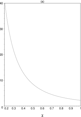
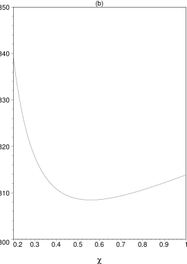
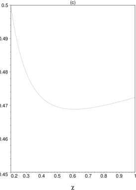
FIG. 1.: Predicted values of (a) $1/\alpha_{3},(b)1/\alpha=1/\alpha_{Y}+1/\alpha_{2}$, and (c) the weak angle $\sin^{2}\theta_{W}=\alpha_{Y}/(\alpha_{2}+\alpha_{Y})$ at the electroweak scale as a function of $\chi$ for $M_{P}^{(4d)}=M_{s}$. Only the contributions $b_{a}({\rm int})$ of the states localized at the brane intersections (as well as the gauge bosons) to the running are included. The experimental values are $\sim$ 8.5, 128, and 0.23, respectively.

It is seen that the predicted value of $\alpha_{3}$ is quite close to the experimental value for $\chi\sim 0.5$ ($1/\alpha_{3}\sim 8.5$). However, $\alpha$ is predicted to be much too small, mainly because of the contributions of the exotic states to the running, while $\sin^{2}\theta_{W}$ is predicted too large by a factor $\sim 2$. (The predicted value of $\sin^{2}\theta_{W}$ at the string scale $M_{s}$ ranges from 0.78 to 0.73 for $\chi$ varying from 0 to $\infty$, while $1/\alpha_{G}\sim 12$ for $\chi\sim 0.5$ and $M_{P}^{(4d)}=M_{s}$.)

Although the predictions for the MSSM gauge couplings are unrealistic, the quasi-hidden sector $Sp$ groups are all asymptotically free. Figure 2 displays the scales at which each $Sp$ group becomes strongly coupled as a function of $\chi$.

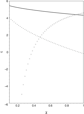
FIG. 2.: Scales $\tau=\frac{1}{2\pi}\ln\frac{M}{M_{Z}}$, where $M$ is the scale at which the $Sp$ group becomes strongly coupled for $M_{P}^{(4d)}=M_{s}$. The curves are $Sp(2)_{A}$ (solid), $Sp(2)_{B}$ (circles), $Sp(4)$ (crosses).

All three groups become strong above the electroweak scale for $M_{P}^{(4d)}=M_{s}$ and $\chi\mathrel{\mathchoice{\lower 2.0pt\vbox{\halign{$\mxth\displaystyle\hfil#\hfil$\cr>\crcr\sim\crcr}}}{\lower 2.0pt\vbox{\halign{$\mxth\textstyle\hfil#\hfil$\cr>\crcr\sim\crcr}}}{\lower 2.0pt\vbox{\halign{$\mxth\scriptstyle\hfil#\hfil$\cr>\crcr\sim\crcr}}}{\lower 2.0pt\vbox{\halign{$\mxth\scriptscriptstyle\hfil#\hfil$\cr>\crcr\sim\crcr}}}}0.4$. For $M_{P}^{(4d)}<M_{s}$ the couplings become strong at higher scales (e.g., $Sp(2)_{B}$ would become strong at around $10^{15}$ GeV for $M_{P}^{(4d)}=M_{s}/3$ and $\chi=0.5$, with possible implications for neutrino mass, as mentioned in Section IV). The implications will be further discussed in Section VI and in [23].

VI Implications of a Strongly Coupled Sector

We have seen that for sufficiently low values of $M_{P}^{(4d)}/M_{s}$ the quasi-hidden sector groups $Sp(2)_{B}$, $Sp(2)_{A}$, and $Sp(4)$ will become strongly coupled above the electroweak scale. This is likely to lead to supersymmetry breaking in the hidden sector, which can be transmitted to the observable sector by supergravity, as well as dilaton/moduli stabilization [23]. Here we will focus on another aspect, i.e., the confinement of free $Sp$ charges, expected in analogy with QCD. In particular, it is plausible to assume that when one of the $Sp(n)$ groups becomes strongly coupled at some scale $M\gg M_{Z}$ any states carrying $Sp(n)$ charges become confined and drop out of the physical spectrum. However, there may be $Sp$-neutral bound state chiral supermultiplets remaining in the spectrum, which may be required to avoid the introduction of anomalies for the remaining gauge groups.

$Sp(4)$ is expected to become strong at a high scale. The only state in the chiral sector with $Sp(4)$ charge is from the $B_{1}C_{2}$ intersection. We denote this state as $\Psi$, which transforms as $(1,2,1,1,4)$ under $SU(3)\times SU(2)\times Sp(2)_{B}\times Sp(2)_{A}\times Sp(4)$. The strong $Sp(4)$ forces may lead to a composite chiral supermultiplet $\Psi^{2}_{AA}$, where the subscript indicates an antisymmetrization in both the $SU(2)$ and $Sp(4)$ indices. $\Psi^{2}_{AA}$ is a total gauge singlet. Whether or not this composite state is formed, the confinement of $\Psi$ does not lead to any anomalies for the residual gauge groups. An anomaly is induced in the $Q_{2}-SU(2)^{2}$ vertex, where $Q_{2}$ is associated with an anomalous $U(1)$ with a massive gauge boson. This can be regarded as a breaking of $Q_{2}$ and is presumably harmless, analogous to to the breaking of the global axial $U(1)$ symmetry in QCD. The four $SU(2)$ doublets contained in $\Psi$ drop out of the renormalization group equations for $SU(2)$ at the decoupling scale, lowering $b_{SU(2)}$ by 2, but this has only a minor impact on the discussion in Section V.

$Sp(2)_{B}$ can become strongly coupled anywhere from a few TeV up to very high scales such as $10^{15}$ GeV, depending on $\chi$ and $M_{P}^{(4d)}/M_{s}$. The fractionally charged $B_{2}C_{1}$ states are charged under $Sp(2)_{B}$. Let us denote them as $\Phi\equiv(3,1,2,1,1)$ and $\Sigma\equiv(1,1,2,1,1)$. By our assumptions, these will be confined at the $Sp(2)_{B}$ scale. The strong $Sp(2)_{B}$ binding might form the composite color triplet $\Phi\Sigma=(3,1,1,1,1)$. This has charge $-1/3$, and would be a candidate for an exotic $SU(2)$-singlet down-type quark, except that it has lepton number $L=1$. Furthermore, if this were the only massless composite, anomalies would be induced in the $Q_{Y}^{3}$ and $Q_{Y}-SU(3)^{2}$ vertices. The anomaly-matching condition suggests that, instead of $\Phi\Sigma$, there is a more complicated spectrum of massless composites. The simplest possibility is that the spectrum consists of

$$E_{4} = \Phi\Sigma\bar{U}$$ (18)

$$N_{4} = \Phi\Sigma\bar{D}$$ (19)

$$U_{4} = \Phi\Sigma\bar{E}$$ (20)

$$D_{4} = \Phi\Sigma\bar{N},$$ (21)

i.e., $\Phi\Sigma$ forms bound states with each member of one of the four families of $SU(2)$-singlet antiquarks and antileptons. The latter do not have to drop out of the spectrum, so the composite $U_{4},D_{4},E_{4}$, and $N_{4}$ are candidates to be the exotic ($SU(2)$-singlet) left-handed partners of the elementary fourth family of antiparticles. This spectrum matches all of the gauge anomalies, although it does lead to a (presumably harmless) $(B+L)-Q_{8}^{2}$ anomaly, again similar to the axial $U(1)$ in QCD.

This binding mechanism seems very plausible from the viewpoint of anomaly matching. However, it is harder to understand from the actual forces between the constituents, since the $\bar{U},\bar{D},\bar{E},\bar{N}$ are not charged under the strong $Sp(2)_{B}$ group. (They do carry other gauge charges.)

The decoupling of $\Phi$ and $\Sigma$ and the appearance of the composite states lead to a net increase of $6/5$ for the $\beta$ function for $1/\alpha_{1}$ at the decoupling scale ($b_{SU(3)}$ and $b_{SU(2)}$ do not change), but this is a small effect for the specific numerical example we have displayed. For example, for $M_{P}^{(4d)}=M_{s}$ and $\chi=0.5$, $Sp(4)$ and $Sp(2)_{B}$ become strong at $\sim 10^{15}$ GeV and $2\times 10^{6}$ GeV, respectively. Including both decouplings, the predicted values of $\alpha^{-1}$ and $\sin^{2}\theta_{W}$ decrease by $\sim 6$ and $0.02$, respectively, compared to those in Figure 1.

$Sp(2)_{A}$ may also become strongly coupled. However, there are no chiral states with $Sp(2)_{A}$ charges.

VII Discussion

In this paper we have described the phenomenological implications of a semi-realistic supersymmetric three family model derived from an orientifold construction. In addition to the MSSM, the model involves an extended gauge structure, including two additional $U(1)^{\prime}$ factors, one of which has family non-universal couplings. There is also a quasi-hidden sector non-abelian group, which becomes strongly coupled above the electroweak scale. There are many exotic chiral supermultiplets, including an exotic ($SU(2)$-singlet) fourth family of quarks and leptons in which the left-chiral states have unphysical fractional electric charges. These are presumably confined by the strong hidden sector interactions, while anomaly constraints imply composite left-chiral states with the correct charges. The right-chiral states are elementary. The Yukawa sector [22] and other aspects of the hidden sector [23] will be presented separately.

As emphasized in the Introduction, none of the models that have been constructed are fully realistic, and it is difficult to know whether the specific features of a given model are hints of possible new TeV scale physics, or merely artifacts of the construction. For that reason, it is useful to contrast some of the features of this orientifold construction with those of a specific heterotic model described in [4]. For convenience, those predictions are described in more detail in the Appendix.

Both models predict additional $U(1)^{\prime}$ gauge symmetries, some of which have family-nonuniversal and therefore flavor changing neutral current couplings. Both are most likely broken at the TeV scale, but have a possibility of being broken at an intermediate scale along a $D$-flat direction. Both also have quasi-hidden nonabelian gauge sectors. This means that while most of the states in the model are charged under one or neither of the gauge sectors, there are a few states which couple to both. (The $U(1)^{\prime}$ also connect the two sectors.) These mixed states have fractional charges like $1/6$ or $\pm 1/2$. A hidden sector is an ideal candidate for dynamical supersymmetry breaking if it is strongly coupled. In the heterotic example the hidden sector groups are not asymptotically free. However, in the orientifold example, the groups are asymptotically free, and may lead to gaugino condensation, dilaton/moduli stabilization, and charge confinement, modifying the low energy spectrum.

Both models involve exotic states, often with no satisfactory means of generating fermion masses. These include additional Higgs doublets and singlets, suggesting such effects as a rich spectrum of Higgs particles, neutralinos, and charginos, perhaps with nonstandard couplings due to mixing and flavor changing effects. The effective $\mu$ terms are either missing or nonstandard. There may also be vector pairs of additional quarks and leptons. In the orientifold case, the left-chiral states are composite and their right-chiral partners elementary. The orientifold model also contains unwanted adjoints. There may be mixing between lepton and Higgs doublets, leading to lepton number violation. This was required in the heterotic case (where baryon number violation was also possible for one flat direction), and optional for the orientifold.

Although the Yukawa couplings have tree-level contributions in string perturbation theory (in orders of $g_{s}$) in the two constructions, they have different origins from the worldsheet perspective. In the orientifold model, the Yukawa couplings arise from non-perturbative effects (worldsheet instantons) in the worldsheet conformal field theory. In the CHL5 model, the Yukawa couplings are tree-level from the worldsheet point of view. We note, however, that in some heterotic string constructions, the quarks, leptons and the Higgs fields are localized at different orbifold fixed points (see e.g., [31] and references therein.). In these constructions, the Yukawa couplings also come from worldsheet instantons. Both constructions can yield masses and mixings for some, but not all, of the fermions, but the details depend on the mechanism of supersymmetry breaking. Neither has an obvious mechanism for a neutrino seesaw, except possibly for the case of an intermediate scale breaking of a $U(1)^{\prime}$.

In the heterotic model the gauge unification predictions are non-standard (and not very successful) due to the combination of exotic particles contributing to the running of the gauge couplings and higher Kač-Moody levels at the string scale. The orientifold predictions are also non-standard: the gauge groups are associated with different branes, and have non-standard moduli-dependent boundary conditions at the string scale, and there are also exotic particles contributing to the running, leading to electroweak couplings that are too small. Resolutions of these difficulties in more successful constructions might involve avoiding these non-standard features, having exotics which fall into complete grand unification multiplets, or invoking cancellations of effects occurring by accident or due to some other mechanism.

As described in the Introduction, there has been considerable study of semi-realistic perturbative heterotic string constructions, including a class of free-fermionic string models which contain the gauge group and matter content of the MSSM [2, 3]. Such constructions generally involve additional gauge factors and many extra matter supermultiplets. However, they also contain an anomalous $U(1)_{A}$ symmetry and a corresponding Fayet-Iliopoulos contribution to the $U(1)_{A}$ $D$-term. Maintaining supersymmetry at the string scale requires that some of the fields in the effective four-dimensional theory must acquire compensating vacuum expectation values (VEVs) near the string scale, while maintaining $F$-flatness and $D$-flatness for the other gauge factors. These break some of the extra gauge symmetries, remove some of the apparently massless states from the low energy effective theory, and require that the theory be restabilized, i.e., the superpotential for the remaining massless states must be recalculated when some of the fields are replaced by their string-scale VEVs. A systematic procedure was developed in [32] to classify the flat directions associated with non-abelian singlet fields. This was used in [4] to investigate the flat directions and related low energy phenomenology in detail for a promising model due originally to Chaudhuri, Hockney, and Lykken [3] (CHL5). Flat directions associated with non-singlets were studied in [33]. The procedures were used to study the flat directions in a class of models due to Faraggi, Nanopoulos, and Yuan [2] in [34].

The features of perturbative heterotic string models are illustrated by the prototypical example of the CHL5 model. These include:

• One or more additional (nonanomalous) $U(1)^{\prime}$ gauge factors. The associated $Z^{\prime}$ gauge boson is typically expected to be lighter than around 1 TeV [27], although for one flat direction studied the breaking could be at an intermediate scale [30]. The $Z^{\prime}$ couplings are family nonuniversal, leading to flavor changing neutral currents (FCNC) [28].

• Additional non-abelian gauge factors. These could, in principle, play a role in dynamical supersymmetry breaking. However, in the model studied the factors do not become strongly coupled below the string scale (i.e, they are not asymptotically free). These extra gauge factors are quasi-hidden, i.e., most matter multiplets transform nontrivially under the standard model $SU(3)\times SU(2)$ group or under the hidden sector group (or neither), but not both. However, there are a few exceptions which are charged under both. The extra $U(1)^{\prime}$ typically couple to both sectors.

• There are many exotic supermultiplets in the model, including an extra $d$-type quark, extra Higgs/lepton doublets, and many non-abelian singlets. For many, there is no mechanism to give a significant mass to the fermions. This is a major flaw of most such models. (One exception, which however has unrealistic Yukawa couplings, is described in [34].) The spectrum includes a number of charge $\pm 1/2$ states. These are all charged under the quasi-hidden sector group, and potentially could disappear from the spectrum if the hidden sector charges are confined [35]. However, as noted above, the hidden sector factors in the CHL5 model are not strongly coupled, so this mechanism does not occur.

• There are more than the two Higgs doublets of the MSSM. In addition to the more complicated Higgs spectrum, there is a possibility of Higgs mediated FCNC. Models with an electroweak scale $U(1)^{\prime}$ can generically provide a natural solution to the $\mu$ problem [26, 27], which is generated dynamically by the VEV of the field that breaks the $U(1)^{\prime}$. However, in the CHL5 model the effective $\mu$ terms are non-canonical, connecting Higgs doublets which generate the $t$ and $b$ masses to others. In the specific examples studied, one of the needed effective $\mu$ terms is absent, leading to an unwanted global symmetry.

• The model has gauge coupling unification. However, the detailed predictions for the low energy couplings differ from the MSSM (and from experiment) because of the additional matter fields as well as higher Kač-Moody levels for the $U(1)$ factors.

• The Yukawa couplings at the string scale are either $g$, $g/\sqrt{2}$, or 0, where $g=O(1)$ is the gauge coupling, allowing large masses for the $t$ and $b$, and the possibility of radiative electroweak breaking. Smaller Yukawa couplings can be associated with higher dimensional operators that become cubic after vacuum restabilization. CHL5 contains $t-b$ and an unphysical $\mu-\tau$ universality, a noncanonical $b-\tau$ relation, and a nontrivial (but unphysical) $d$ quark texture for one flat direction.

• The models violate $R$-parity and lepton number (due to mixing between lepton and Higgs doublets), so there is no stable neutralino. Baryon number is violated for one flat direction, leading to proton decay and $n-\bar{n}$ oscillations (with rates that cannot be calculated without resolving the problem of the massless exotics).

• There is no obvious mechanism for a neutrino seesaw except for the cases in which one of the $U(1)^{\prime}$ gauge factors is broken at an intermediate scale [30].

• When phenomenological soft supersymmetry breaking parameters are introduced by hand at the string scale, one can calculate the symmetry breaking and the spectrum of the Higgs and supersymmetry particles. One can obtain a sufficiently large $Z^{\prime}$ mass (e.g., $>$ 700 GeV) and small $Z-Z^{\prime}$ mixing (e.g., $<$ 0.005) for somewhat tuned values of the soft parameters. The large $Z^{\prime}$ mass scale is set by the soft breaking parameters, implying a spectrum quite different from most of the parameter space of the MSSM: typically, the squark and slepton masses are in the TeV range (except possibly for the third family), but there is a richer spectrum of Higgs particles, charginos, and neutralinos [36].

REFERENCES

- [1] For reviews, see, e.g., B. R. Greene, Lectures at Trieste Summer School on High Energy Physics and Cosmology (1990); F. Quevedo, hep-th/9603074; A. E. Faraggi, hep-ph/9707311; Z. Kakushadze, G. Shiu, S. H. Tye and Y. Vtorov-Karevsky, Int. J. Mod. Phys. A 13, 2551 (1998); G. Cleaver, M. Cvetič, J. R. Espinosa, L. L. Everett, P. Langacker and J. Wang, Phys. Rev. D 59, 055005 (1999) and references therein.
- [2] A. E. Faraggi, D. V. Nanopoulos and K. Yuan, Nucl. Phys. B 335, 347 (1990).
- [3] S. Chaudhuri, G. Hockney and J. Lykken, Nucl. Phys. B 469, 357 (1996).
- [4] G. Cleaver, M. Cvetič, J. R. Espinosa, L. L. Everett, P. Langacker and J. Wang, Phys. Rev. D 59, 055005 (1999); Phys. Rev. D 59, 115003 (1999).
- [5] C. Angelantonj, M. Bianchi, G. Pradisi, A. Sagnotti and Ya.S. Stanev, Phys. Lett. B. 385, 96 (1996).
- [6] M. Berkooz and R.G. Leigh, Nucl. Phys. B 483, 187 (1997).
- [7] Z. Kakushadze and G. Shiu, Phys. Rev. D 56, 3686 (1997); Nucl. Phys. B 520, 75 (1998); Z. Kakushadze, Nucl. Phys. B 512, 221 (1998).
- [8] G. Shiu and S.-H.H. Tye, Phys. Rev. D 58, 106007 (1998).
- [9] Z. Kakushadze, G. Shiu and S. H. Tye, Nucl. Phys. B 533, 25 (1998); Phys. Rev. D 58, 086001 (1998).
- [10] G. Aldazabal, A. Font, L.E. Ibáñez and G. Violero, Nucl. Phys. B 536, 29 (1999).
- [11] Z. Kakushadze, Phys. Lett. B 434, 269 (1998); Phys. Rev. D 58, 101901 (1998); Nucl. Phys. B 535, 311 (1998).
- [12] M. Cvetič, M. Plümacher and J. Wang, JHEP 0004, 004 (2000).
- [13] M. Klein, R. Rabadán, JHEP 0010, 049 (2000).
- [14] M. Cvetič, A. M. Uranga and J. Wang, Nucl. Phys. B 595, 63 (2001).
- [15] M. Cvetič, G. Shiu and A. M. Uranga, Phys. Rev. Lett. 87, 201801 (2001); Nucl. Phys. B 615, 3 (2001).
- [16] M. Cvetič, G. Shiu and A. M. Uranga, “Chiral type II orientifold constructions as M theory on holonomy spaces,”, hep-th/0111179.
- [17] M. Berkooz, M. R. Douglas and R. G. Leigh, Nucl. Phys. B 480, 265 (1996).
- [18] R. Blumenhagen, L. Goerlich, B. Kors and D. Lust, JHEP 0010, 006 (2000).
- [19] G. Aldazabal, S. Franco, L. E. Ibáñez, R. Rabadán and A. M. Uranga, J. Math. Phys. 42, 3103 (2001); JHEP 0102, 047 (2001).
- [20] R. Blumenhagen, B. Körs and D. Lüst, JHEP 0102, 030 (2001).
- [21] C. Angelantonj, I. Antoniadis, E. Dudas and A. Sagnotti, Phys. Lett. B 489, 223 (2000).
- [22] M. Cvetič, G. Shiu, and P. Langacker, UPR-0991T, to appear.
- [23] M. Cvetič, P. Langacker, and J. Wang, work in progress.
- [24] C. Angelantonj and R. Blumenhagen, Phys. Lett. B 473, 86 (2000).
- [25] L. E. Ibáñez, F. Marchesano and R. Rabadán, JHEP 0111, 002 (2001).
- [26] D. Suematsu and Y. Yamagishi, Int. J. Mod. Phys. A 10, 4521 (1995).
- [27] M. Cvetič, D. A. Demir, J. R. Espinosa, L. L. Everett and P. Langacker, Phys. Rev. D 56, 2861 (1997) [Erratum-ibid. D 58, 119905 (1997)].
- [28] P. Langacker and M. Plümacher, Phys. Rev. D 62, 013006 (2000).
- [29] See J. Erler and P. Langacker, Phys. Rev. Lett. 84, 212 (2000), and references theirin.
- [30] G. Cleaver, M. Cvetič, J. R. Espinosa, L. L. Everett and P. Langacker, Phys. Rev. D 57, 2701 (1998); P. Langacker, Phys. Rev. D 58, 093017 (1998).
- [31] M. Cvetič, Phys. Rev. Lett. 59, 1795 (1987).
- [32] G. Cleaver, M. Cvetič, J. R. Espinosa, L. L. Everett and P. Langacker, Nucl. Phys. B 525, 3 (1998); G. Cleaver, M. Cvetič, J. R. Espinosa, L. L. Everett and P. Langacker, Nucl. Phys. B 545, 47 (1999).
- [33] M. Cvetič, L. Everett, P. Langacker and J. Wang, JHEP 9904, 020 (1999).
- [34] G. B. Cleaver, A. E. Faraggi, D. V. Nanopoulos and J. W. Walker, Nucl. Phys. B 593, 471 (2001); Nucl. Phys. B 620, 259 (2002).
- [35] See C. Coriano, A. E. Faraggi and M. Plümacher, Nucl. Phys. B 614, 233 (2001) and references theirin.
- [36] L. L. Everett, P. Langacker, M. Plümacher and J. Wang, Phys. Lett. B 477, 233 (2000).