Self-energy correction to the bound-electron $g$ factor in H-like ions

Abstract

The one-loop self-energy correction to the $1s$ electron $g$ factor is evaluated to all orders in $Z\alpha$ with an accuracy, which is essentially better than that of previous calculations of this correction. As a result, the uncertainty of the theoretical prediction for the bound-electron $g$ factor in H-like carbon is reduced by a factor of 3. This improves the total accuracy of the recent electron-mass determination [Beier et al. Phys. Rev. Lett. 88, 011603 (2002)]. The new value of the electron mass is found to be $m_{e}=0.000\,548\,579\,909\,3\,(3)$ u.

PACS number(s): 31.30.Jv, 12.20.Ds

Spectacular progress in high-precision measurements of the bound-electron $g$ factor for the hydrogen-like carbon [1, 2] and the related theoretical investigations recently provided a new independent determination of the electron mass [3]. It yields

$$m_{e}(g)=0.000\,548\,579\,909\,2\,(4)\ \mbox{\rm u}\,.$$

This result agrees with the 1998 CODATA value [4]

$$m_{e}(\mbox{\rm CODATA})=0.000\,548\,579\,911\,0\,(12)\ \mbox{\rm u}\,$$

within 1.5 standard deviations but is three times more precise. The uncertainty of the electron-mass value of [3] originates equally from the theoretical result for the bound-electron $g$ factor and from the experimental value for the ratio of the electronic Larmor precession frequency and the cyclotron frequency of the ion in the trap. Therefore, any advance in theoretical or experimental investigations will improve the accuracy of the electron-mass value. However, for significant progress one needs to reduce both the theoretical and experimental uncertainties. From the experimental side, an increase of the accuracy by an order of magnitude is anticipated in the near future, as well as an extension of the measurements to higher-$Z$ systems [5]. Investigations of the bound-electron $g$ factor in high-$Z$ systems are of particular importance since they can provide a new determination of the fine structure constant [6, 5], nuclear magnetic moments [5], and nuclear charge radii. They would also create a good possibility for testing the magnetic sector of QED in a strong Coulomb field.

From the theoretical point of view, the leading error of the bound-electron g-factor value for H-like carbon comes from the one-loop self-energy correction. Reducing this uncertainty is the aim of the present investigation. The second major error is due to the two-loop binding QED correction that is known at present only to the lowest order in $Z\alpha$ [6, 7, 8]. To reduce that uncertainty is a serious problem. However, recent progress in calculations of two-loop QED corrections to the Lamb shift, both within the $Z\alpha$ expansion [9] and to all orders in $Z\alpha$ [10], allows us to hope that its solution might be possible in the near future. An important feature of studying the bound-electron $g$ factor is a relative weakness of nuclear effects. Unlike the hyperfine splitting, where a large effect of distribution of the magnetic moment over the nucleus complicates the identification of one-loop QED effects, for the bound-electron $g$ factor, the uncertainty due to nuclear effects is of the order of two-loop binding QED corrections even in the high-$Z$ region. In addition, as shown in [11], the finite-nuclear-size effect can be largely cancelled in a specific difference of the bound-electron $g$ factors for H- and Li-like ions with the same nucleus. Therefore, this difference can be (in principle) calculated up to a very high accuracy. This fact makes the bound-electron $g$ factor very promising for testing two-loop QED effects by comparing theory and experiment.

The one-loop self-energy correction to the $1s$ $g$ factor was first evaluated by Blundell et al. [12] and by Persson et al. [13]. The latter work was extended by Beier and co-workers [14], whose result was used in the electron-mass determination [3].

Formal expressions for the one-loop self-energy correction to the bound-state g factor are well-known (see, e.g., [15]). The whole correction is conveniently divided into three parts, which are referred to as the irreducible ($\Delta g_{\rm ir}$), the reducible ($\Delta g_{\rm red}$) and the vertex ($\Delta g_{\rm ver}$) contribution. The irreducible part is given by

$$\Delta g_{\rm ir}=\frac{2}{b}\langle a|\Sigma_{R}(\varepsilon_{a})|\delta a\rangle\,,$$ (1)

where $\Sigma_{R}$ denotes the renormalized self-energy operator, and $a$ indicates the initial state. We use the relativistic units ($\hbar=c=1$) and the Heaviside charge unit [$\alpha=e^{2}/(4\pi)$, $e<0$] throughout this Letter. The perturbed wave function $|\delta a\rangle$ is

$$|\delta a\rangle\ =\sum_{\varepsilon_{n}\neq\varepsilon_{a}}\frac{|n\rangle\langle n|\delta V|a\rangle}{\varepsilon_{a}-\varepsilon_{n}}\,,$$ (2)

where $\delta V({\bf x})=-e{\mbox{\boldmath$\alpha$}}\cdot{\bf A}_{\rm cl}({\bf x})$, ${\bf A}_{\rm cl}$ denotes the classical homogeneous magnetic field, ${\bf A}_{\rm cl}({\bf x})=[{\cal H}\times{\bf x}]/2$, $b$ is defined by $\Delta E=b\,\Delta g$, $b=\mu_{0}m_{a}{\cal H}$, $\mu_{0}=|e|/(2m)$ is the Bohr magneton, and $m_{a}$ is the angular-momentum projection of the initial state. The reducible contribution is represented as

$$\Delta g_{\rm red}=\frac{1}{b}\langle a|\delta V|a\rangle\langle a|\left.\frac{\partial}{\partial\varepsilon}\Sigma_{R}(\varepsilon)\right|_{\varepsilon=\varepsilon_{a}}|a\rangle\,,$$ (3)

and the vertex part is given by

$$\Delta g_{\rm ver}=\frac{1}{b}\sum_{n_{1}n_{2}}\frac{i}{2\pi}\int^{\infty}_{-\infty}d\omega\,\frac{\langle n_{1}|\delta V|n_{2}\rangle\langle an_{2}|I(\omega)|n_{1}a\rangle}{[\varepsilon_{a}-\omega-\varepsilon_{n_{1}}(1-i0)][\varepsilon_{a}-\omega-\varepsilon_{n_{2}}(1-i0)]}\,,$$ (4)

where $I(\omega)=e^{2}\alpha^{\mu}\alpha^{\nu}D_{\mu\nu}(\omega)$ is the operator of the electron-electron interaction, $D_{\mu\nu}(\omega)$ stands for the photon propagator, and $\alpha^{\mu}=(1,{\mbox{\boldmath$\alpha$}})$ are the Dirac matrices. In order to avoid large numerical cancellations, it is convenient to calculate the vertex and the reducible part together. We indicate the sum of these two contributions with the subscript "vr", $\Delta g_{\rm vr}=\Delta g_{\rm ver}+\Delta g_{\rm red}$.

Now we turn to the numerical evaluation of these contributions. We perform our calculations in the Feynman gauge and both for the point and the extended nucleus. In the latter case, the hollow-shell nuclear model was utilized. Since calculations for the point nucleus are easier from the technical point of view and because of smallness of the finite-nuclear-size effect, we later discuss mainly the point-nucleus evaluation. Convergence of the extended-nucleus value to the point-nucleus result for small values of $Z$ served as one of the checkups for our numerical procedure. The calculation of the irreducible part is quite straightforward. For the point nucleus, the perturbed wave function $|\delta a\rangle$ can be found analytically by employing the generalized virial relations for the Dirac equation [16]. The corresponding explicit expressions can be found in [17]. The numerical evaluation of the non-diagonal matrix element of the self-energy operator was carried out similarly to that for the self-energy correction to the hyperfine structure [18], within the Green-function technique. The partial-wave expansion converges well in that case, and taking into account 30-50 partial waves is sufficient for getting the required accuracy (with the rest of the series estimated by polynomial fitting). As an additional cross-check for the evaluation of the irreducible part, we also utilized a modified renormalization procedure, where the energy of the one-potential term is shifted from its physical value (for more details we refer the reader to [18]).

The numerical evaluation of the vertex and reducible parts is more problematic. The standard way to treat corrections of this kind is to separate terms in which bound electron propagators are replaced with free propagators. We refer to this part as the 0-potential contribution $\Delta g_{\rm vr}^{(0)}$. This term contains ultraviolet divergences that can be covariantly separated and cancelled in momentum space. The remainder $\Delta g_{\rm vr}^{(1+)}$ is ultraviolet finite and can be calculated directly in coordinate space, as in [12]. However, it turns out that due to a strong cancellation between the reducible and the vertex part, the contribution of high partial waves is relatively large for low $Z$, and the corresponding expansion is slowly converging. For gaining better control over the partial-wave summation, in [13, 14] it was proposed to separate from $\Delta g_{\rm vr}^{(1+)}$ a part containing (besides an interaction with the magnetic field) one Coulomb interaction with the nucleus in electron propagators, the so-called 1-potential contribution $\Delta g_{\rm vr}^{(1)}$. The authors demonstrated that the partial-wave expansion of the remainder (the many-potential contribution $\Delta g_{\rm vr}^{(2+)}$) is converging much better than that for $\Delta g_{\rm vr}^{(1+)}$. For the evaluation of the 1-potential term, a separate numerical scheme was developed in [13, 14], based on an analytical treatment of radial integrals. This allowed the authors to extend the partial-wave summation up to $l_{\rm max}=120$. However, the unevaluated tail of the expansion still yields a significant contribution in that case. In order to get the accuracy, ascribed to the 1-potential term in [14] for carbon, one should estimate the tail of the series with an uncertainty of about 1%. This is a potentially dangerous point of this numerical evaluation.

The central point of the present calculation is a different treatment of the 1-potential term. We evaluate it directly in momentum space without utilizing the partial-wave expansion and, in this way, eliminate the uncertainty due to the estimation of the tail of the series. The next difference from the calculations [13, 14] consists in the treatment of the magnetic interaction in momentum space. The Fourier transform of the classical magnetic potential involves the gradient of a $\delta$ function,

$${\bf A}_{\rm cl}({\bf q})=-\frac{i}{2}(2\pi)^{3}[{\cal H}\times{\mbox{\boldmath$\nabla$}}_{{\bf q}}\delta^{3}({\bf q})]\,.$$ (5)

In [13, 14], the $\delta$ function was replaced by a continuous Gaussian function with a small but finite regulator. In our evaluation of the 0- and 1-potential terms, we employ directly (5) and evaluate the corresponding corrections after integration by parts. (For the 0-potential term, the same approach was utilized earlier in [12].) In case of the 0-potential term, this treatment requires additional analytical work, but finally, instead of a five-dimensional numerical integration (as in [13, 14]), we end up with a single integral that can be evaluated up to an arbitrary precision. The analytical part of the evaluation of the 1-potential term is quite tedious, but the overall $\delta$ function simplifies the calculation greatly. Finally, the 1-potential term is represented by a four-dimensional integral, whose numerical evaluation is relatively easy.

The calculation of the many-potential term was carried out in a manner similar to that in [18]. The many-potential part was represented by a point-by-point difference of the unrenormalized, the 0-potential, and the 1-potential term. In addition, we also subtract the infrared-divergent contribution of the reference state from the vertex and reducible parts. This contribution was then evaluated separately, carrying out the $\omega$ integration analytically and explicitly cancelling divergences in the sum of the reducible and the vertex part. Care should be taken in the evaluation of the many-potential correction, since a large numerical cancellation occurs in the point-by-point difference. In order to avoid the appearance of pole terms that lead to additional numerical cancellations, we employ the following contour of the $\omega$ integration: $(\varepsilon_{0}-i\infty,\varepsilon_{0}-i0]+[\varepsilon_{0}-i0,-i0]+[i0,\varepsilon_{0}+i0]+[\varepsilon_{0}+i0,\varepsilon_{0}+i\infty)$, rather than simply the integration over the imaginary axis. The parameter $\varepsilon_{0}$ in the definition of the contour can be varied. In actual calculations its value was taken to be about $Z\alpha\,\varepsilon_{a}$ for low $Z$. The summation over partial waves was carried out up to $|\kappa_{\rm max}|=20$-$35$, and the tail of the series was estimated by polynomial fitting.

The results of our numerical evaluation are presented in Table I. In order to isolate the one-loop binding self-energy correction, we subtract from the total self-energy correction the free-electron value $\alpha/\pi$ [19]. The resulting binding correction is compared with the data from [14]. For all cases except for $Z=20$, the results agree with each other within the given error bars. A more detailed comparison is presented in Table II for two most important cases, carbon and oxygen. A certain deviation can be observed for the 1-potential and many-potential contributions, that is largely cancelled in the sum. We do not have any explanation of this fact at present. As an additional checkup of our calculation, we fitted our data for the binding correction and compared the result for the leading $(Z\alpha)^{2}$ term with the analytical value [8] $a_{20}=1/6=0.1666\ldots$. Our fitting yields $a_{20}=0.1667(2)$. Finally, we separate the higher-order contribution $F_{\rm h.o.}(Z\alpha)$ that incorporates terms of order $(Z\alpha)^{4}$ and higher,

$$\Delta g_{\rm SE}=\frac{\alpha}{\pi}\left[1+\frac{1}{6}(Z\alpha)^{2}+(Z\alpha)^{4}F_{\rm h.o.}(Z\alpha)\right]\,.$$ (6)

The results for the higher-order contribution are represented in Fig. 1, together with those from [14]. A least-squares fit of our data to the form

$$F_{\rm h.o.}(Z\alpha)=a_{41}\ln(Z\alpha)+a_{40}+(Z\alpha)[\cdots]$$ (7)

yields $a_{41}=-7.0(8)$ and $a_{40}=-10(2)$.

In Table III we present individual contributions to the $1s$ electron $g$ factor for two most important cases, H-like carbon and oxygen. The Dirac point-nucleus value and the free-electron part of the one-loop QED correction are evaluated utilizing the recommended value for the fine-structure constant from [4]. The finite-nuclear-size correction is calculated numerically and is in good agreement with the previous evaluations [14, 20]. The so-called "electric-loop" part of the one-loop vacuum-polarization correction is also re-evaluated in this work. The corresponding results agree with the earlier numerical [13, 14] and analytical [21] calculations. The remaining part of the vacuum-polarization ("magnetic-loop") correction is shown to be negligible for the case under consideration [21]. The $\alpha^{2}$ QED correction includes the existing $Z\alpha$ expansion terms for the QED correction of second order in $\alpha$ [6, 7] and the known free-QED terms of higher orders in $\alpha$ (see, e.g., [15]). Its relative uncertainty was estimated as the ratio of the part of the one-loop QED correction that is beyond the $(Z\alpha)^{2}$ approximation, to the part that is within the $(Z\alpha)^{2}$ approximation, multiplied by a factor of 1.5. The recoil correction incorporates the total recoil contribution of first order in $m/M$, calculated to all orders in $Z\alpha$ in [22], and the known corrections of orders $(m/M)^{2}$ and $\alpha(m/M)$ [23].

In summary, our evaluation of the one-loop self-energy correction for the $1s$ electron $g$ factor in H-like ions improves the accuracy of the theoretical prediction for carbon by a factor of 3 and for oxygen by a factor of 2. This reduces the total uncertainty of the electron-mass determination of [3]. The new value for the electron mass is found to be

$$m_{e}=0.000\,548\,579\,909\,29\,(29)(8)\,,$$ (8)

where the first uncertainty originates from the experimental value for the ratio of the electronic Larmor precession frequency and the cyclotron frequency of the ion in the trap, and the second error comes from the theoretical value for the bound-electron $g$ factor.

We would like to thank Th. Beier for valuable discussions and, in particular, for communicating the details of the extrapolation procedure of the partial-wave expansion used in his calculation. Valuable conversations with H.-J. Kluge and W. Quint are gratefully acknowledged. This study was supported in part by the Russian Foundation for Basic Research (project no. 01-02-17248), by the program "Russian Universities" (project no. UR.01.01.072), and by GSI. The stay of V.Y. in Paris is supported by the Ministère de l’Education Nationale et de la Recherche. Laboratoire Kastler Brossel is Unité Mixte de Recherche de l’École Normale Supérieure, du CNRS et de l’Université P. et M. Curie.

TABLE I.: Various contributions to the one-loop self-energy correction to the $1s$ electron $g$ factor for H-like ions. All values are absolute contributions to the $g$ factor ($1/\alpha=137.035\,989\,5$) and presented in units of $10^{-6}$ (ppm). The point and the extended nuclear model are indicated with labels "pnt." and "ext.", respectively. The binding correction is obtained by subtraction of the free-electron value $\alpha/\pi$ from the total self-energy correction $\Delta g_{\rm SE}$. Only the total numerical error of the present evaluation is indicated.

$Z$	$\Delta g_{\rm ir}$		$\Delta g_{\rm vr}^{(0)}$		$\Delta g_{\rm vr}^{(1)}$		$\Delta g_{\rm vr}^{(2+)}$		$\Delta g_{\rm SE}$		Binding		Binding		Ref. [14]
	(pnt.)		(pnt.)		(pnt.)		(pnt.)		(pnt.)		(pnt.)		(ext.)		(ext.)
1	1.	52923	2320.	77563	0.	50250	0.	03305	2322.	84041(10)	0.	02078(10)			0.	0208(9)
2	5.	20641	2316.	00970	1.	55757	0.	13053	2322.	90421(10)	0.	08458(10)			0.	0844(9)
3	10.	52313	2309.	28506	2.	91759	0.	28869	2323.	01447(10)	0.	19484(10)			0.	1944(9)
4	17.	21614	2300.	99753	4.	45945	0.	50260	2323.	17572(10)	0.	35609(10)			0.	3555(9)
5	25.	10745	2291.	41521	6.	10392	0.	76661	2323.	39319(10)	0.	57356(10)			0.	5732(9)
6	34.	06468	2280.	73799	7.	79535	1.	07460	2323.	67262(10)	0.	85299(10)			0.	8528(9)
8	54.	78171	2256.	69788	11.	16571	1.	79701	2324.	44231(10)	1.	62268(10)	1	.62267(10)	1.	6225(10)
10	78.	74380	2229.	82629	14.	34905	2.	61754	2325.	53668(12)	2.	71705(12)	2	.71702(12)	2.	7159(10)
12	105.	51170	2200.	79829	17.	21623	3.	48376	2327.	00998(15)	4.	19035(15)	4	.19030(15)	4.	1907(12)
15	150.	23525	2154.	28732	20.	77184	4.	75746	2330.	05187(20)	7.	23224(20)	7	.23212(20)	7.	231(1)
18	199.	76448	2105.	29703	23.	34254	5.	85654	2334.	26059(25)	11.	44096(25)	11	.44067(25)	11.	442(2)
20	235.	17646	2071.	71454	24.	49971	6.	41815	2337.	80886(30)	14.	98923(30)	14	.98870(30)	15.	04(1)

TABLE II.: Various contributions to the one-loop self-energy correction to the $1s$ electron $g$ factor for H-like carbon and oxygen in the present evaluation and by Beier et al. Units are ppm. Our numerical values correspond to the point nuclear model. Due to the smallness of the finite-nuclear-size effect, a different treatment of the nucleus in the two calculations does not influence the term-by-term comparison.

	$\Delta g_{\rm ir}$		$\Delta g_{\rm vr}^{(0)}$		$\Delta g_{\rm vr}^{(1)}$		$\Delta g_{\rm vr}^{(2+)}$		$\Delta g_{\rm SE}$
$Z$=6, this work	34.	06468(4)	2280.	73799	7.	79535(2)	1.	07460(9)	2323.	67262(10)
$Z$=6, [14]	34.	0647(4)	2280.	7380(3)	7.	7945(1)	1.	0752(1)	2323.	6724(9)
$Z$=8, this work	54.	78171(4)	2256.	69788	11.	16571(2)	1.	79701(9)	2324.	44231(10)
$Z$=8, [14]	54.	7815(4)	2256.	6979(3)	11.	1646(2)	1.	7981(1)	2324.	4421(10)

TABLE III.: The $1s$ electron $g$ factor in H-like carbon and oxygen.

	${}^{12}{\rm C}^{5+}$		${}^{16}{\rm O}^{7+}$
Dirac value (point)	1.	998 721 354 4	1.	997 726 003 1
Fin. nucl. size	0.	000 000 000 4	0.	000 000 001 5
QED, order $(\alpha/\pi)$	0.	002 323 663 9(1)	0.	002 324 415 6(1)
QED, order $(\alpha/\pi)^{2}$	-0.	000 003 516 2(3)	-0.	000 003 517 1(6)
Recoil	0.	000 000 087 6	0.	000 000 117 0
Total	2.	001 041 590 1(3)	2.	000 047 020 1(6)

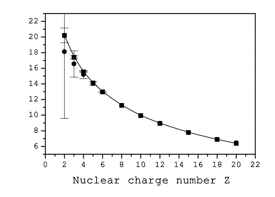
FIG. 1.: The higher-order contribution to the $1s$ electron $g$ factor for H-like ions $F_{\rm h.o.}(Z)$, defined by (6). The squares indicate our numerical values and the circles stand for the results of Beier et al.

REFERENCES

- [1] N. Hermanspahn, H. Häffner, H.-J. Kluge, W. Quint, S. Stahl, J. Verdú, and G. Werth, Phys. Rev. Lett. 84, 427 (2000).
- [2] H. Häffner, T. Beier, N. Hermanspahn, H.-J. Kluge, W. Quint, S. Stahl, J. Verdú, and G. Werth, Phys. Rev. Lett. 85, 5308 (2000).
- [3] T. Beier, H. Häffner, N. Hermanspahn, S.G. Karshenboim, H.-J. Kluge, W. Quint, S. Stahl, J. Verdú, and G. Werth, Phys. Rev. Lett. 88, 011603 (2002).
- [4] P.J. Mohr and B.N. Taylor, Rev. Mod. Phys. 72, 351 (2000).
- [5] G. Werth, H. Häffner, N. Hermanspahn, H.-J. Kluge, W. Quint, J. Verdú, in The Hydrogen Atom, eds. S.G. Karshenboim et al. (Springer, Berlin, 2001), p. 204.
- [6] S.G. Karshenboim, in The Hydrogen Atom, eds. S.G. Karshenboim et al. (Springer, Berlin, 2001), p. 651; E-print, hep-ph/0008227 (2000).
- [7] A. Czarnecki, K. Melnikov, and A. Yelkhovsky, Phys. Rev. A 63, 012509 (2001).
- [8] H. Grotch, Phys. Rev. Lett. 24, 39 (1970).
- [9] K. Pachucki, Phys. Rev. A 63, 042503 (2001).
- [10] V.A. Yerokhin and V.M. Shabaev, Phys. Rev. A 64, 062507 (2001).
- [11] V.M. Shabaev, D.A. Glazov, M.D. Shabaeva, V.A. Yerokhin, G. Plunien, and G. Soff, Phys. Rev. A, in press.
- [12] S.A. Blundell, K.T. Cheng, J. Sapirstein, Phys. Rev. A 55, 1857 (1997).
- [13] H. Persson, S. Salomonson, P. Sunnergren, I. Lindgren, Phys. Rev. A 56, R2499 (1997).
- [14] T. Beier, I. Lindgren, H. Persson, S. Salomonson, P. Sunnergren, H. Häffner, and N. Hermanspahn, Phys. Rev. A 62, 032510 (2000).
- [15] T. Beier, Phys. Rep. 339, 79 (2000).
- [16] V.M. Shabaev, J. Phys. B 24, 4479 (1991).
- [17] V.M. Shabaev, Phys. Rev. A 64, 052104 (2001).
- [18] V.A. Yerokhin and V.M. Shabaev, Phys. Rev. A 64, 012506 (2001).
- [19] J. Schwinger, Phys. Rev. 73, 416 (1948).
- [20] D.A. Glazov, V.M. Shabaev, Phys. Lett. A, in press.
- [21] S. Karshenboim, V.G. Ivanov, and V.M. Shabaev, Zh. Eksp. Teor. Fiz. 120, 546 (2001) [JETP 93, 477 (2001)].
- [22] V.M. Shabaev and V.A. Yerokhin, Phys. Rev. Lett. 88, 091801 (2002).
- [23] A.P. Martynenko and R.N. Faustov, Zh. Eksp. Teor. Fiz. 120, 539 (2001) [JETP 93, 471 (2001)].