Solar Neutrinos: Global Analysis with Day and Night Spectra from SNO

P. C. de Holanda¹ and A. Yu. Smirnov^1,2

(1) The Abdus Salam International Centre for Theoretical Physics, I-34100 Trieste, Italy
(2) Institute for Nuclear Research of Russian Academy of Sciences, Moscow 117312, Russia

We perform global analysis of the solar neutrino data including the day and night spectra of events at SNO. In the context of two active neutrino mixing, the best fit of the data is provided by the LMA MSW solution with $\Delta m^{2}=6.15\cdot 10^{-5}$ eV², $\tan^{2}\theta=0.41$, $f_{B}=1.05$, where $f_{B}$ is the boron neutrino flux in units of the corresponding flux in the Standard Solar Model (SSM). At $3\sigma$ level we find the following upper bounds: $\tan^{2}\theta<0.84$ and $\Delta m^{2}<3.6\cdot 10^{-4}$ eV². From $1\sigma$-interval we expect the day-night asymmetries of the charged current and electron scattering events to be: $A_{DN}^{CC}=3.9^{+3.6}_{-2.9}\%$ and $A_{DN}^{ES}=2.1^{+2.1}_{-1.4}\%$. The only other solution which appears at $3\sigma$-level is the VAC solution with $\Delta m^{2}=4.5\cdot 10^{-10}$ eV², $\tan^{2}\theta=2.1$ and $f_{B}=0.75$. The best fit point in the LOW region, with $\Delta m^{2}=0.93\cdot 10^{-7}$ eV² and $\tan^{2}\theta=0.64$, is accepted at $99.95\%$ ($3.5\sigma$) C.L. . The least $\chi^{2}$ point from the SMA solution region, with $\Delta m^{2}=4.6\cdot 10^{-6}$ eV² and $\tan^{2}\theta=5\cdot 10^{-4}$, could be accepted at $5.5\sigma$-level only. In the three neutrino context the influence of $\theta_{13}$ is studied. We find that with increase of $\theta_{13}$ the LMA best fit point shifts to larger $\Delta m^{2}$, mixing angle is practically unchanged, and the quality of the fit becomes worse. The fits of LOW and SMA slightly improve. Predictions for KamLAND experiment (total rates, spectrum distortion) have been calculated.

Pacs numbers: 14.60.Lm 14.60.Pq 95.85.Ry 26.65.+t

1 Introduction

The SNO data [1, 2, 3, 4, 5] is the breakthrough in a long story of the solar neutrino problem. With high confidence level we can claim that solar neutrinos undergo the flavor conversion

$$\nu_{e}\rightarrow\nu_{\mu},\nu_{\tau}~{}~{}{\rm or/and}~{}~{}\bar{\nu}_{\mu},\bar{\nu}_{\tau}.$$ (1)

Moreover, non-electron neutrinos compose larger part of the solar neutrino flux at high energies (also partial conversion to sterile neutrinos is not excluded). The main issue now is to identify the mechanism of neutrino conversion.

There are several important pieces of new information from the recent SNO publication [3, 4, 5]:

1. Measurements of the energy spectra with low threshold (as well as angular distribution) of events allow to extract information on the neutrino neutral current (NC), charged current (CC), as well as electron scattering (ES) event rates. In particular, in assumption of absence of distortion, one gets for the ratio of the NC/CC event rates:

$$\frac{NC}{CC}=2.9\pm 0.4$$ (2)

which deviates from 1 by about $5\sigma$.

2. Measurements of the day and night energy spectra allow to find the D-N asymmetries of different classes of events. Under constraint that total flux has no D-N asymmetry one gets for CC event rate [4]

$$A^{CC}_{DN}=7.0\pm 4.9~{}^{+1.5}_{-1.4}\%.$$ (3)

3. No substantial distortion of the neutrino energy spectrum has been found.

4. Solutions of the solar neutrino problem based on pure active - sterile conversion, $\nu_{e}\rightarrow\nu_{s}$, are strongly disfavored.

These results further confirm earlier indications of $\nu_{\mu}-,\nu_{\tau}-$ appearance from comparison of fluxes determined from the charged current event rate in the SNO detector [1, 2], and the $\nu e-$scattering event rate obtained by the Super-Kamiokande (SK) collaboration [6, 7, 8].

Implications of the new SNO results for different solutions (see [9, 10] for earlier studies) can be obtained immediately by comparison of the results (2, 3) with predictions from the best fit points of different solutions [11, 12, 13, 14, 15, 16, 17]. In particular, for the LMA solution the best fit prediction $NC/CC=3.3$ (for lower threshold) [15] is slightly higher than (2). So, new results should move the best fit point to larger values of mixing angles. The expected day-night asymmetry in the best fit point, $\sim 6\%$, is well within the interval (3). Clearly new data further favor this solution.

For LOW solution: $NC/CC=2.4$ [15] in the best fit point, which is $1\sigma$ (experimental) lower than the central SNO value. The expected asymmetry was lower than (3), therefore this solution is somewhat less favored, and SNO tends to shift the allowed region to smaller values of $\theta$ which correspond to smaller survival probability.

Implications of new SNO results have been studied in [18, 19, 20, 21, 22]. In this paper we continue this study. We perform global analysis of all available data including the SNO day and night energy spectra of events, and the latest data from Super-Kamiokande and SAGE. We identify the most plausible solutions and study their properties.

The paper is organized as follows: In Section 2 we describe features of our analysis. In Section 3 we present results of the $\chi^{2}-$ test, and construct the pull-off diagrams for various observables. In Section 4 we determine the regions of solutions and describe their properties. In Section 5 we consider the effect of $\theta_{13}$ on the solutions. In Section 6 we study the predictions to KamLAND for the parameters given by the found solutions. The conclusion is given in Section 7.

2 Global analysis of the solar neutrino data

In this section we describe main ingredients of our analysis. We follow the procedure of analysis developed in previous publications [9, 10, 15, 16, 23].

2.1 Input data

We use the following set of the experimental results:

1) Three rates (3 d.o.f.):

(i) the $Ar-$production rate $Q_{Ar}$ measured by the Homestake experiment [24],

(ii) the $Ge-$production rate, $Q_{Ge}$, from SAGE [25],

(iii) the combined $Ge-$production rate from GALLEX and GNO [26].

2) The zenith-spectra measured by Super-Kamiokande [6] during 1496 days of operation. The data consists of 8 energy bins with 7 zenith angle bins in each, except for the first and last energy bins, which makes 44 data points. We use the experimental errors given in [7] and we treat the correlation of systematic uncertainties as in [16]. Following the procedure outlined in [10] we do not include the total rate of events in the SK detector, which is not independent from the spectral data.

3) From SNO, we use the day and the night energy spectra of all events [5]. We follow procedure described in [5]. Additional information on how to treat the systematic uncertainties was given by [27].

Altogether there are 81 data points.

2.2 Neutrino Fluxes

All solar neutrino fluxes (but the boron neutrino flux) are taken according to SSM BP2000 [28]. We use the boron neutrino flux as free parameter. We define dimensionless parameter

$$f_{B}\equiv\frac{F_{B}}{F_{B}^{SSM}},$$ (4)

where the SSM boron neutrino flux is taken to be $F^{SSM}_{B}=5.05\cdot 10^{6}$ cm^-2 s^-1. For the $hep-$neutrino flux we take fixed value $F_{hep}=9.3\times 10^{3}$ cm^-2 s^-1 [28, 29] .

2.3 Neutrino mixing and conversion

We perform analysis of data in terms of mixing of two flavor neutrinos and three flavor neutrinos.

In the case of two neutrinos there are two oscillation parameters: the mass squared difference, $\Delta m^{2}$, and the mixing parameter $\tan^{2}\theta$. So, we have three fit parameters: $\Delta m^{2}$, $\tan^{2}\theta$, $f_{B}$, and therefore 81(data points) - 3 = 78 d.o.f.

In the case of three neutrino mixing we adopt the mass scheme which explains the solar and the atmospheric neutrino data. In this scheme the mass eigenstates $\nu_{1}$ and $\nu_{2}$ are splitted by the solar $\Delta m^{2}_{12}$, whereas the third mass eigenstate, $\nu_{3}$, is separated by larger mass split related to the atmospheric $\Delta m^{2}_{13}$. Matter effect influences very weakly mixing (flavor content) of the third mass eigenstate. The effect of third neutrino is reduced then to the averaged vacuum oscillations. In this case, the survival probability equals

$$P_{ee}=\cos^{4}\theta_{13}P_{ee}^{(2)}+\sin^{4}\theta_{13},$$ (5)

where $\sin\theta_{13}\equiv U_{e3}$ describes the mixing of electron neutrino in the third mass eigenstate and $P_{ee}^{(2)}$ is the two neutrino oscillation probability characterized by $\tan^{2}\theta_{12}$, $\Delta m_{12}^{2}$ and the effective matter potential reduced by factor $\cos^{2}\theta_{13}$ (see e.g. [30, 31] for previous studies).

In general, in the three neutrino case the fit parameters are $\tan^{2}\theta_{12}$, $\Delta m_{12}^{2}$, $\sin\theta_{13}$ and $f_{B}$. However, here for illustrative purpose we take fixed value of $\theta_{13}$ near its upper bound. So, the number of degrees of freedom is the same as in the two neutrino case.

2.4 Statistical analysis

We perform the $\chi^{2}$ test of various oscillation solutions by calculating

$$\chi^{2}_{global}=\chi^{2}_{rate}+\chi^{2}_{SK}+\chi^{2}_{SNO},$$ (6)

where $\chi^{2}_{rate}$, $\chi^{2}_{SK}$ and $\chi^{2}_{SNO}$ are the contributions from the total rates, from the Super-Kamiokande zenith spectra and the SNO day and night spectra correspondingly. Each of the entries in Eq.(6) is the function of three parameters ($\Delta m^{2}$, $\tan^{2}\theta$, $f_{B}$).

Some details of treatment of the systematic errors are given in the Appendix.

The uncertainties of contributions from different components of the solar neutrino flux (pp-, Be-, B- etc.) to $Ge$-production rate due to uncertainties of the cross-section of the detection reaction $\nu_{e}-Ga$ correlate. Similarly, uncertainties of contributions to $Ar$ production rate due to uncertainty in $\nu_{e}-Cl$ cross-section correlate. Following [32] we have taken into account these correlations.

2.5 Cross-checks. Comparison with other analysis

We have checked our results performing two additional fits:

1) To check our treatment of the SK data we have performed global analysis taking from SNO only the CC-rate. That corresponds to the analysis done in [7, 8]. We get very good agreement of the results.

2) To check our treatment of the latest SNO data we have performed analysis using the day and night spectra from SNO, as in [4]. We have reproduced the results of paper [4] with a good accuracy.

Our input set of the data differs from that used in other analyses: We include more complete and up-dated information. SNO [4] uses the SK day and night spectra measured after 1258 days. In contrast, we use preliminary SK zenith spectra measured during 1496 days. In [19] the NC/CC ratio and the D-N asymmetry at SNO where included in the analysis. The analysis done by Barger et al [18] uses the same data set we do.

3 $\chi^{2}$ test

In this section we describe the results of fit for two neutrino mixing.

In Table 1 we show the best fit values of parameters $\Delta m^{2}$, $\tan^{2}\theta$, $f_{B}$ for different solutions of the solar neutrino problem. We also give the corresponding values of $\chi^{2}_{min}$ and the goodness of the fit.

The absolute $\chi^{2}$ minimum, $\chi^{2}=65.2$ for 78 d.o.f., is in the LMA region. The vacuum oscillation is the next best. It, however, requires $\sim 30\%$ lower boron neutrino flux. The LOW solution has slightly higher $\chi^{2}$. The SMA gives a very bad fit.

Table 1: Best-fit values of the parameters $\Delta m^{2}$, $\tan^{2}\theta$ and $f_{B}$, as well as the minimum $\chi^{2}$ and the corresponding g.o.f. for various global solutions. The number of degrees of freedom is 78.

Solution	$\Delta m^{2}$/$\rm eV^{2}$	$\tan^{2}\theta$	$f_{B}$	$\chi^{2}_{min}$	g.o.f.
LMA	$6.15\times 10^{-5}$	0.41	1.05	65.2	85%
VAC	$4.5\times 10^{-10}$	2.1	0.749	74.9	58%
LOW	$0.93\times 10^{-7}$	0.64	0.908	77.6	49%
SMA	$4.6\times 10^{-6}$	$0.5\times 10^{-3}$	0.57	99.7	4.9%

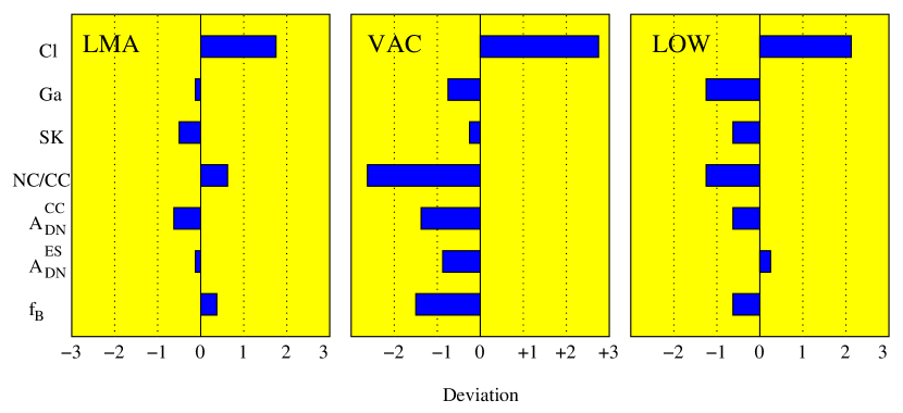
Figure 1: Pull-off diagrams for global solutions. Shown are deviations of predictions from experimentally measured values for the $Ar-$production rate, $Ge-$production rate, SK rate, the day-night asymmetries at SK and SNO. The pull-offs are expressed in the units of 1 standard deviation, $1\sigma$.

In order to check the quality of the fits we have calculated predictions for the available observables in the best fit points of the global solutions (see Table 1). Using these predictions we have constructed the “pull-off” diagrams (fig. 1) which show deviations, $D_{K}$, of the predicted values of observables $K$ from the central experimental values expressed in the $1\sigma$ unit:

$$D_{K}\equiv\frac{K_{bf}-K_{exp}}{\sigma_{K}},~{}~{}~{}~{}K\equiv Q_{Ar},~{}Q_{Ge},~{}NC/CC,~{}R_{\nu e},~{}A_{DN}^{SK},A_{DN}^{CC}.$$ (7)

Here $\sigma_{K}$ is the one sigma standard deviation for a given observable $K$. $R_{\nu e}$ is the reduced total rate of events at SK. We take the experimental errors only: $\sigma_{K}=\sigma_{K}^{exp}$.

According to Fig. 1 only the LMA solution does not have strong deviations of predictions from the experimental results. LOW and VAC solutions give worse fit to the data.

4 Parameters of solutions

We define the solution regions by constructing the contours of constant (68, 90, 95, 99, 99.73 %) confidence level with respect of the absolute minimum in the LMA region. Following the same procedure as in [10], for each point in the $\Delta m^{2}$, $\tan^{2}\theta$ plane we find minimal value $\chi^{2}_{min}(\Delta m^{2},\tan^{2}\theta)$ varying $f_{B}$. We define the contours of constant confidence level by the condition

$$\chi^{2}_{min}(\Delta m^{2},\tan^{2}\theta)=\chi^{2}_{min}(LMA)+\Delta\chi^{2}~{},$$ (8)

where $\chi^{2}_{min}(LMA)=65.2$ is the absolute minimum in the LMA region and $\Delta\chi^{2}$ is taken for two degrees of freedom.

4.1 LMA

Recent SNO data further favors the LMA MSW solution (see e.g. [33]). In the best fit point we get

$$\Delta m^{2}=6.15\cdot 10^{-5}~{}{\rm eV}^{2},~{}~{}~{}\tan^{2}\theta=0.41,~{}~{}~{}f_{B}=1.05.$$ (9)

The value of $\Delta m^{2}$ is slightly higher than that found in the SNO analysis and higher than in our previous analysis [15]. The shift is mainly due to updated SK results which show smaller D-N asymmetry than before. Large SNO asymmetry which would push $\Delta m^{2}$ to smaller values is still statistically insignificant. The mixing angle is shifted to larger values (in comparison with previous analysis) due to smaller ratio of the NC/CC event rates. The boron neutrino flux is 5% higher than central value in the SSM: $F_{B}=f_{B}\cdot F_{B}^{SSM}=5.32\cdot 10^{6}$ cm^-2 s^-1 being however within $1\sigma$ deviation and well in agreement with SNO measurements.

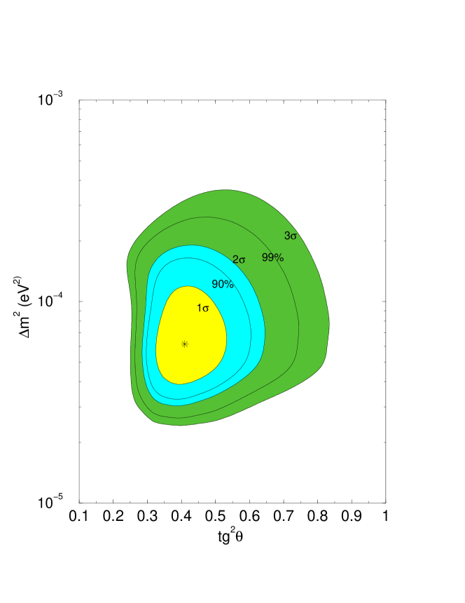
Figure 2: The global LMA MSW solution. The boron neutrino flux is considered as free parameter. The best fit point is marked by a star. The allowed regions are shown at 1$\sigma$, 90% C.L., 2$\sigma$, 99% C.L. and 3$\sigma$.

The CL contours (see fig. 2) shrink substantially as compared with previous determination [11, 12, 13, 14, 15, 16, 17].

From fig. 2 we find the following bounds on oscillations parameters:

1) $\Delta m^{2}$ is rather sharply restricted from below by the day-night asymmetry at SK: $\Delta m^{2}>2.3\cdot 10^{-5}$ eV² at 99.73% C.L. .

2) The upper limits on $\Delta m^{2}$ for different confidence levels equal:

$$\Delta m^{2}\leq\left\{\begin{array}[]{ll}1.2\times 10^{-4}~{}{\rm eV}^{2},&~{}~{}68.27\%~{}{\rm C.L.}\\ 1.9\times 10^{-4}~{}{\rm eV}^{2},&~{}~{}95\%~{}{\rm C.L.}\\ 3.6\times 10^{-4}~{}{\rm eV}^{2},&~{}~{}99.73\%~{}{\rm C.L.}\\ \end{array}\right..$$ (10)

All these limits are stronger than the CHOOZ [37] bound which appears for maximal mixing at $\Delta m^{2}\sim 8\times 10^{-4}{\rm eV}^{2}$.

3) The upper limit on mixing angle becomes substantially stronger than before:

$$\tan^{2}\theta<\left\{\begin{array}[]{ll}0.53{}{}&68.27\%~{}~{}{\rm C.L.}\\ 0.65{}{}&95\%~{}~{}{\rm C.L.}\\ 0.84{}{}&99.73\%~{}~{}{\rm C.L.}\\ \end{array}\right.$$ (11)

Maximal mixing is allowed at $\sim 4\sigma$ level for $\Delta m^{2}=(5-7)\cdot 10^{-5}$ eV².

Notice that the SNO data alone exclude maximal mixing at about 3$\sigma$: the data determine now rather precisely the NC/CC ratio which is directly related to $\sin^{2}\theta$. Also observed Germanium production rate as well as Argon production rate disfavor maximal mixing (see fig. 3 and 4).

So, now we have strong evidence that solar neutrino mixing significantly deviates from maximal value. One can introduce the deviation parameter [36]

$$\epsilon\equiv 1-2\sin^{2}\theta.$$ (12)

From our analysis we get

$$\epsilon>0.08,~{}~{}~{}(3\sigma).$$ (13)

That is, at $3\sigma$: $\epsilon>\sin^{2}\theta_{c}$, where $\theta_{c}$ is the Cabibbo angle. This result has important theoretical implications.

4) lower limit on mixing :

$$\tan^{2}\theta>0.23,~{}~{}~{}~{}99\%~{}{\rm C.L.}.$$ (14)

is changed weakly.

In fig. 3-6 we show the grids of predicted values for various observables.

According to the pull-off diagram and figs. 3-6, the LMA solution reproduces observables at $\sim 1\sigma$ or better. The largest deviation is for the $Ar-$production rate: the solution predicts $1.6\sigma$ larger rate than the Homestake result.

The best fit point value and $3\sigma$ interval for Ge production rate equal

$$Q_{Ge}=70.5~{}SNU,~{}~{}~{}Q_{Ge}=(63-84)SNU,~{}~{}~{}~{}~{}3\sigma.$$ (15)

Notice that at maximal mixing $Q_{Ge}<63$ SNU which is $2\sigma$ away from the combined experimental result.

4.2 VAC

In the best fit point we get $\chi^{2}=74.9$ and:

$$\chi^{2}(VAC)-\chi^{2}(LMA)=9.7.$$ (16)

So, this solution is accepted at $3\sigma$ level. Notice that the solution appears in the dark side of the parameter space which means that some matter effect is present. This solution was “discovered” in 1998 and its properties have already been described in the literature. Clearly it does not predict any day-night asymmetry. The solution requires rather low ($1.6\sigma$) Boron neutrino flux and gives rather poor description of rates (see fig. 1). In particular, 2.7$\sigma$ higher Ar-production rate and 2.6$\sigma$ lower NC/CC ratio are predicted. Imposing the SSM restriction on this flux leads to exclusion of this VAC solution at $3\sigma$ level.

4.3 Any chance for SMA?

We find that the best fit point from the SMA region has $\chi^{2}=99.8$. For the difference of $\chi^{2}$ we have:

$$\chi^{2}(SMA)-\chi^{2}(LMA)=34.5.$$ (17)

That is, SMA is accepted at $5.5\sigma$ only. Moreover, the solution requires about $3\sigma$ lower boron neutrino flux than in the SSM. It predicts negative Day-Night asymmetry: $A_{DN}^{CC}=-0.93\%$.

Our results are in qualitative agreement with those in [18], where even larger $\Delta\chi^{2}$ has been obtained.

We find that the $\chi^{2}$ increases weakly with $\tan^{2}\theta$ up to $\tan^{2}\theta=1.5\cdot 10^{-3}$, where $\chi^{2}\sim 105$.

Is SMA excluded? We find that very bad fit is due to latest SNO measurements of day and night spectra. We have checked that the analysis of the same set of data but CC rate from SNO only (2001 year) instead of spectrum leads to the best fit values $\Delta m^{2}=4.8\cdot 10^{-6}~{}{\rm eV}^{2}$, $\tan^{2}\theta=3.9\cdot 10^{-4}$ and $f_{B}=$ and $\chi^{2}(SMA)-\chi^{2}(LMA)=11$ in a good agreement with results of similar analysis in [8]. Since CC SNO data are in a good agreement with new NC/CC result, just using the NC/CC does not produce substantial change of quality of the SMA fit [19]. So it is the spectral data which give large contribution to $\chi^{2}$.

The SMA solution with very small mixing provides rather good description of the SK data: the rate and spectra. The (reduced) rate $R\equiv OBS/SSM$ of the ES events can be written as

$$[ES]=f_{B}[P_{ee}(1-r)+r],$$ (18)

where $r\approx 0.16$ is the ratio of $\nu_{\mu}-e$ to $\nu_{e}-e$ cross-sections. Taking $R_{ES}=0.45$ and $f_{B}=0.58$ we find the effective survival probability: $P_{ee}=0.73$. Then, for reduced CC event rate we get $[CC]=f_{B}P_{ee}=0.425$ - close to the ES rate, and moreover,

$$NC/CC\approx 1/P_{ee}=1.37$$ (19)

which is substantially smaller then the observed quantity (2). So, one predicts in this case a suppressed contribution of the NC events to the total rates. Correspondingly, significant distortion of the energy spectrum of events is expected with smaller than observed rate at low energies and higher rate at high energies.

This problem with SNO could be avoided for larger mixing: $\tan^{2}\theta>1.5\cdot 10^{-3}$ (in fact, imposing the SSM restriction on the boron neutrino flux leads to the shift of the best fit point to larger $\theta$). In this case, however serious problems with SK data appear, namely, with spectrum distortion and zenith angle distribution. Strong day-night asymmetry is predicted for the Earth core-crossing bin. Previous analysis which used SK day and night spectra could not realize the latter problem.

Notice that the SNO data alone do not disfavor SMA with large $\tan^{2}\theta=(1.5-2)\cdot 10^{-3}$. This region, however is strongly disfavored by SK.

Zenith angle distribution can give a decisive check of the SMA solution. The SNO night data could be divided into two bins: “mantle” and “core”. Concentration of the night excess of rate in the core bin [34] due to parametric enhancement of oscillations for the core crossing trajectories [35], would be the evidence of the SMA solution with relatively large mixing: $\tan^{2}\theta=(1.5-2)\cdot 10^{-3}$. However, the SK zenith spectra do not show any excess of the “core” bin rate which testify against this possibility.

Probably some unknown systematics could improve the SMA fit. Otherwise, this solution is practically excluded.

4.4 LOW starts to disappear?

In the best fit point we get $\chi^{2}=78.9$, so that

$$\chi^{2}(LOW)-\chi^{2}(LMA)=12.4$$ (20)

which is slightly beyond the $3\sigma$ range. In contrast with other analyses, LOW does not appear at $3\sigma$ level. Notice that in the SNO analysis [4] the LOW solution exists marginally at $3\sigma$ level. Inclusion of the SK data which contain information about zenith angle distribution (zenith spectra) worsen the fit (this effect has also been observed in [13]).

The LOW solution gives rather poor fit of total rates. In the best fit point we get $2.1\sigma$ larger $Ar-$production rate and $1.2\sigma$ lower $Ge-$production rate. For the day-night asymmetry of the CC-events we predict $A_{DN}^{CC}=3.5\%$ and for ES events: $A_{DN}^{CC}=2.7\%$.

5 Three neutrino mixing: effect of $\theta_{13}$

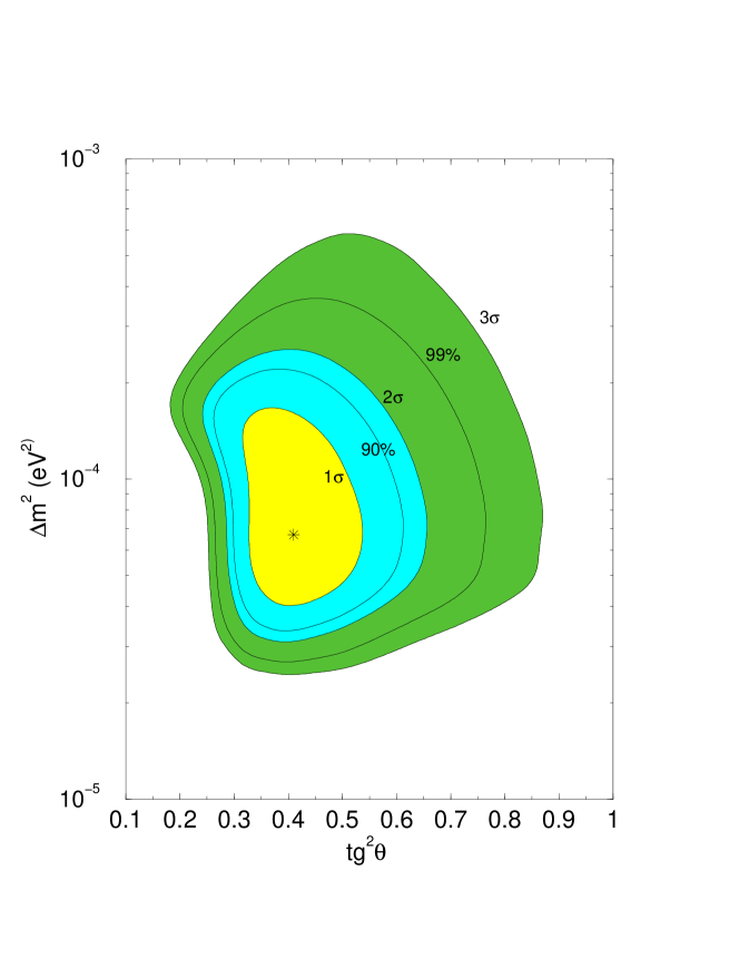
Figure 7: Global LMA solution for $\sin^{2}\theta_{13}=0.04$. The boron neutrino flux is considered as free parameter. The best fit point is marked by a star. The allowed regions are shown at 1$\sigma$, 90% C.L., 2$\sigma$, 99% C.L. and 3$\sigma$.

Results of the global analysis in the three neutrino context are shown in fig. 7. To illustrate the effect of third neutrino we use the three neutrino survival probability (5) for fixed value $\sin^{2}\theta_{13}=0.04$ near the upper bound from the CHOOZ experiment [37]. The number of degrees of freedom is the same as in the previous analysis.

We find the best fit point:

$$\Delta m^{2}_{12}=6.7\cdot 10^{-5}{\rm eV}^{2},~{}~{}~{}~{}\tan^{2}\theta=0.41,~{}~{}~{}~{}f_{B}=1.09$$ (21)

with $\chi^{2}=66.2$. The best fit value of $\Delta m^{2}_{12}$ is slightly higher than that in the two neutrino case, whereas the mixing angle is unchanged. The solution requires slightly higher value of the boron neutrino flux. The changes are rather small, however, as a tendency, we find that with increase of $\theta_{13}$ the fit becomes worser in comparison with $2\nu-$ case. For $\sin^{2}\theta_{13}=0.04$ we get $\Delta\chi^{2}=1.0$.

In fig. 7 we show the contours of constant confidence level constructed with respect to the best fit point (21). The contours changed weakly for low mass values $\Delta m^{2}_{12}<10^{-4}$ ${\rm eV}^{2}$ and there are significant changes for $\Delta m^{2}_{12}>10^{-4}$ ${\rm eV}^{2}$. In particular, the $3\sigma$ upper bound on $\Delta m^{2}_{12}$ is $\Delta m^{2}_{12}<5.8\cdot 10^{-4}$ ${\rm eV}^{2}$; the lower $3\sigma$ bound on mixing: $\tan^{2}\theta_{12}=0.18$ (compare with numbers in the Table 1). Notice, however, that changes are substantially weaker if the contours are constructed with respect to the absolute minimum for $\theta_{13}=0$ (6).

The changes can be easily understood from the following analytical consideration.

The contribution of the last term in the probability (5) is negligible: for largest possible value of $\theta_{13}$ it is below 0.5%. So, we can safely use approximation:

$$P_{ee}\approx\cos^{4}\theta_{13}P_{ee}^{(2)}\approx(1-2\sin^{2}\theta_{13})P_{ee}^{(2)}.$$ (22)

Mainly the effect of $\theta_{13}$ is reduced to overall suppression of the survival probability. The suppression factor can be as small as 0.90 - 0.92.

In the fit with the free boron neutrino flux, the observables at high energies ( $>$ 5 MeV) are determined by the following reduced rates

$$[NC]\equiv\frac{NC}{NC^{SSM}}=~{}~{}f_{B},$$

$$[CC]\equiv\frac{CC}{CC^{SSM}}=~{}~{}f_{B}\cos^{4}\theta_{13}P^{(2)}_{ee},$$

$$[ES]\equiv\frac{ES}{ES^{SSM}}=~{}~{}f_{B}[\cos^{4}\theta_{13}P^{(2)}_{ee}(1-r)+r].$$ (23)

As far as the fit of experimental data on CC-events are concerned (SNO, SK, and partly, Homestake), the effects of $\theta_{13}$ is simply reduced to renormalization of the boron neutrino flux:

$$f_{B}\rightarrow\frac{f_{B}}{\cos^{4}\theta_{13}}$$ (24)

without change of the oscillation parameters $\Delta m_{12}$ and $\theta_{12}$. The dependence of the parameters on $\theta_{13}$ appears via the ratios of rates, which do not depend on $f_{B}$. From (23) we find

$$\cos^{4}\theta_{13}\frac{[NC]}{[CC]}\approx\frac{1}{P^{(2)}_{ee}}$$ (25)

$$\frac{\cos^{4}\theta_{13}}{r}\left[\frac{[ES]}{[CC]}-(1-r)\right]\approx\frac{1}{P^{(2)}_{ee}}.$$ (26)

So, the effect of $\theta_{13}$ is equivalent to decrease of the ratios [NC]/[CC] and [ES]/[CC]. According to fig. 7, this shifts the allowed regions to larger $\Delta m_{12}$ and $\theta_{12}$.

For low energy measurements (Gallium experiments), sensitive to the pp-neutrino flux, which is known rather well, the increase of $\theta_{13}$ should be compensated by increase of the survival probability. This may occur due to increase of $\Delta m_{12}$ or/and decrease of $\tan^{2}\theta_{12}$.

For $\Delta m^{2}_{12}<10^{-4}$ ${\rm eV}^{2}$ the boron neutrino spectrum is in the bottom of suppression pit and the low energy neutrinos are on the adiabatic edge. In the fit, the increase of $\theta_{13}$ is compensated by the increase of $f_{B}$ and $\Delta m^{2}_{12}$. For $\Delta m^{2}_{12}>10^{-4}$ ${\rm eV}^{2}$, the spectrum is in the region where conversion is determined mainly by averaged vacuum oscillations with some matter corrections: $P^{(2)}_{ee}\sim(1-0.5\sin^{2}2\theta_{12})$. The dependence on $\Delta m^{2}_{12}$ is very weak which explains substantial enlargement of the allowed region to large values of $\Delta m^{2}_{12}$. The effect of $\theta_{13}$ can be compensated by decrease of $\theta_{12}$ which explains expansion of the region toward smaller $\tan^{2}\theta_{12}$.

For LOW solution increase of $\theta_{13}$ leads to improvement of the fit, so that this solution appears (for $\sin^{2}\theta_{13}=0.4$) at 3$\sigma$ level with respect to best fit point (21). Also for the SMA solution the effect of $\theta_{13}$ leads to slight improvement of the fit.

6 Predictions for KamLAND

Next step in developments will be probably related to operation of the KamLAND experiment [38]. Both total rate of events above the effective threshold $T_{eff}$ and the energy spectrum of events will be measured.

We characterize the effect of the oscillation disappearance by the ratio of the total number of events with visible energy above $T_{eff}$:

$$R_{Kam}=\frac{1}{N_{0}}\int_{T_{eff}}\int_{T^{\prime}}\int_{E}dEdT^{\prime}dT\sum F_{i}P_{i}\frac{d\sigma}{dT}f(T,T^{\prime})\,,$$ (27)

where $F_{i}$ is the flux from $i$ reactor, $P_{i}$ is the survival probability for neutrinos from $i$ reactor, $\sigma$ is the cross-section of the detection reaction, $f(T,T^{\prime})$ is the energy resolution. $N_{0}$ is the rate without oscillations ($P_{i}=1$).

In our calculations we used the energy spectra of reactor neutrinos from [39, 40]. The differential cross-section of the $p+\overline{\nu_{e}}\rightarrow n+e^{+}$ reaction, is taken from  [41]. The parameters of the 16 nuclear reactors, maximal thermal power, distance from the reactor to the detector, etc., are given in [38]. We used the Gaussian form for the energy resolution function $f(T,T^{\prime})$ with $\sigma/E=5\%/\sqrt{E(MeV)}$, and $T_{eff}=2.6$ MeV as the threshold for the visible energy  [42].

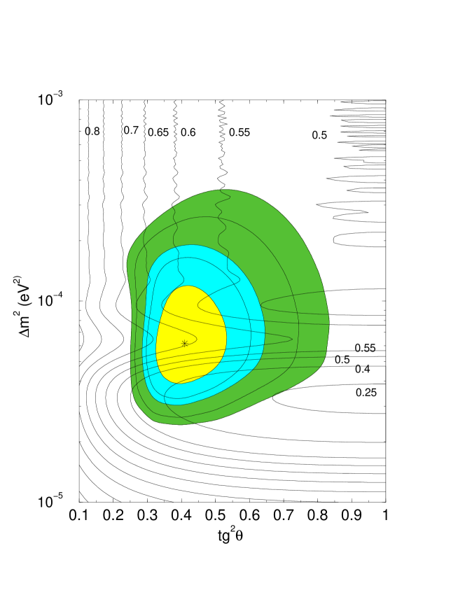
Figure 8: Lines of constant total suppression at KamLAND. In the best fit point: $R_{Kam}=0.65$.

In fig. 8 we show the contours of constant suppression factor in the $\Delta m^{2}-\tan^{2}\theta$ plot. In the best fit point

$$R_{Kam}=0.65\,,$$ (28)

and in the $1\sigma$ region: $R_{Kam}=0.4-0.7$.

Notice that the best fit point is in the range of lowest sensitivity of the total rate on $\tan^{2}\theta$. If e.g. $R_{Kam}$ is measured with $8\%$ accuracy which would correspond to $R_{Kam}=0.65\pm 0.05$, we get from the fig. 8 that any mixing in the interval $\tan^{2}\theta=0.12-1.0$ is allowed.

The suppression factor strongly depends on $\Delta m^{2}$ in the range below the best fit point and this dependence is very weak for $\Delta m^{2}>10^{-4}$ eV². No bound on $\Delta m^{2}$ from the allowed region can be obtained by measurements of the total rate.

The distortion of the visible energy spectrum depends on $\Delta m^{2}$ strongly. In fig. 9 we show the spectrum for different values of $\Delta m^{2}$. There is a shift of maximum to large $E$ with increase of $\Delta m^{2}$. For the best fit value of $\Delta m^{2}$ the maximum is at $E\approx 3.5$ MeV. The most profound effect of oscillations is the suppression of rate at high energies. For instance, for $E\approx 5$ MeV the suppression factor is smaller than 1/2.

7 Conclusions

We find that the LMA MSW solution with parameters $\Delta m^{2}\sim 6.15\cdot 10^{-5}$ eV² and $\tan^{2}\theta=0.41$ gives the best fit to the data. The solution reproduces well the zenith spectrum measured by SK and the day and night spectra at SNO. It is in a very good agreement with SSM flux of the boron neutrino: $f_{B}=1.05$.

The recent SNO results together with zenith spectra results from SK slightly shifted the best fit point to larger $\Delta m^{2}$ and $\theta$. At the same time the allowed regions of oscillation parameters shrunk, leading to important, and statistically significant, upper bounds on mixing angle and $\Delta m^{2}$. Now we have strong evidence that “solar” mixing is non-maximal, and moreover, deviation from maximal mixing is rather large. We find that QuasiVacuum oscillation solution with $\Delta m^{2}=4.5\cdot 10^{-10}$ eV² and mixing in the dark side is the only other solution accepted at $3\sigma$ level, provided that the boron neutrino flux is about 30% below the SSM value.

The LOW solution is accepted at slightly higher than $3\sigma$ level and it reappears at $3\sigma$ level if $\theta_{13}$ is included.

The SMA solution gives very bad fit of the data especially the SNO spectra predicting rather small contribution of the NC events in comparison with CC events.

We find that $\theta_{13}$ produces rather small effect on the solutions even with new high statistics data. As a tendency we see that inclusion of the $\theta_{13}$ effect worses fit of the data in the LMA region, and shifts the best fit point to larger $\Delta m^{2}_{12}$.

We have found predictions for the KamLAND experiment: in the best fit point one expects the suppression factor for total signal $\sim 0.6-0.7$ and the spectrum distortion with substantial suppression in the high energy part.

Appendix

The systematics uncertainties were treated according to [23]. Writing the total counting rate in SNO as a sum over different contributions and different spectral bins, we have:

$$R_{j}=\sum_{i=1,5}R_{ij}\,,$$ (29)

where the index $j$ stands for the different spectral bins and $i$ runs over the five contributions to the SNO data (CC, NC, ES, neutron background and low energy background). We assume that all systematic uncertainties of the SNO result are the uncertainties in the theoretical prediction. These uncertainties can be written in terms of the systematics uncertainties of the input parameters of experiment ($X_{k}$):

$$\sigma^{2}_{j_{1},j_{2}}(TH)=\sum_{k=1,14}\frac{\partial R_{j_{1}}}{\partial lnX_{k}}\frac{\partial R_{j_{2}}}{\partial lnX_{k}}(\Delta lnX_{k})^{2}.$$ (30)

We take the systematic uncertainties from [5]. The different systematic uncertainties are added in quadrature.

Eq.(30) can be written in terms of the different contributions $R_{ij}$  (29) as:

$$\sigma^{2}_{j_{1},j_{2}}(TH)=\sum_{i_{1}=1,5}\sum_{i_{2}=1,5}R_{i_{1}j_{1}}R_{i_{2}j_{2}}\sum_{k=1,14}\alpha_{i_{1},j_{1},k}\alpha_{i_{2},j_{2},k}(\Delta lnX_{k})^{2}\,,$$ (31)

where we have introduced the parameters $\alpha_{i,j,k}$:

$$\alpha_{i,j,k}\equiv\frac{\partial lnR_{i,j}}{\partial lnX_{k}}.$$ (32)

These parameters are numerically estimated by changing the response function of the detector through changes in the parameters $X_{k}$.

Figure 3: Lines of constant $Ge$-production rate (number at the curves in SNU) in the LMA region. In the best fit point: $R_{Ge}=70.5$ SNU.

Figure 4: The same as in Fig 3, but for the Ar-production rate. In the best fit point: $R_{Ar}=2.95$ SNU. The dependence of $f_{B}$ on oscillation parameters is taken into account.

Figure 5: Lines of constant NC/CC ratio in the LMA region. In the best fit point: $NC/CC=3.15$.

Figure 6: Lines of constant day-night asymmetry of CC events. In the best fit point: $A_{DN}^{CC}=3.9\%$.

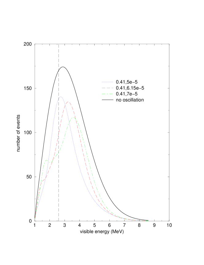
Figure 9: Spectral distortion for three different values on $\Delta m^{2}$, including the best fit point of our analysis.

References

- [1] Q. R. Ahmad et al., SNO collaboration, Phys. Rev. Lett. 87:071301, 2001.
- [2] A. B. McDonald, Proc. of the 19th Int. Conf. on Neutrino Physics and Astrophysics, Neutrino 2000 , Sudbury, Canada 2000, Nucl. Phys. B (Proc. Suppl.) 91 (2001) 21.
- [3] Q. R. Ahmad et al., SNO collaboration, nucl-ex/0204008.
- [4] Q. R. Ahmad et al., SNO collaboration, nucl-ex/0204009.
-
[5]
“How to use the SNO Solar Neutrino Spectral Data”, at
http://www.sno.phy.queensu.ca/. - [6] S. Fukuda et al. (Super-Kamiokande collaboration) Phys. Rev. Lett. 86: 5651, 2001; Phys. Rev. Lett. 86: 5656, 2001.
- [7] M.B. Smy, the proceedings of 3rd Workshop on Neutrino Oscillations and Their Origin (NOON 2001), Kashiwa, Japan, 5-8 Dec 2001; hep-ex/0202020.
- [8] M.B. Smy, the proceedings of NO-VE International Workshop on Neutrino Oscillations in Venice, Venice, Italy, 24-26 Jul 2001. *Venice 2001, Neutrino oscillations* 35-42; hep-ex/0108053.
- [9] J. N. Bahcall, P.I. Krastev, A. Yu. Smirnov, Phys. Rev. D 62 (2000) 093004, Phys. Rev. D 63 (2001) 053012.
- [10] J. N. Bahcall, P.I. Krastev, A. Yu. Smirnov, JHEP 5 (2001) 15.
- [11] V. Barger, D. Marfatia and K. Whisnant, Phys. Rev. Lett. 88:011302, 2002.
- [12] G.L. Fogli, E. Lisi, D. Montanino and A. Palazzo, Phys. Rev. D64:093007, 2001; hep-ph/0203138.
- [13] J. N. Bahcall, M. C. Gonzalez-Garcia, Carlos Peña-Garay, JHEP 0108:014, 2001; JHEP 0204:007, 2002.
- [14] A. Bandyopadhyay, S. Choubey, S. Goswami, K. Kar, Phys.Lett.B519:83-92,2001.
- [15] P. I. Krastev, A.Yu. Smirnov, Phys. Rev. D65:073022, 2002.
- [16] A. M. Gago, et al, Phys. Rev. D65:073012, 2002.
- [17] P. Aliani, V. Antonelli, M. Picariello, E. Torrente-Lujan, hep-ph/0111418.
- [18] V. Barger, D. Marfatia, K. Whisnant, B.P. Wood, hep-ph/0204253.
- [19] John N. Bahcall, M.C. Gonzalez-Garcia, Carlos Peña-Garay, hep-ph/0204314.
- [20] Abhijit Bandyopadhyay, Sandhya Choubey, Srubabati Goswami, D.P. Roy, hep-ph/0204286.
- [21] P. Creminelli, G. Signorelli A. Strumia, hep-ph/0102234, v3 22 April 2002 (addendum 2).
- [22] P. Aliani, et al, hep-ph/0205053.
- [23] G.L. Fogli and E. Lisi, Astropart. Phys. 3, 185 (1995).
- [24] B. T. Cleveland et al Astroph. J. 496 (1998) 505; K. Lande et al, in Neutrino 2000 [2], p.50.
- [25] J.N. Abdurashitov et al. (SAGE collaboration), astro-ph/0204245.
- [26] C. M. Cattadori et al., in Proceedings of the TAUP 2001 Workshop, (September 2001), Gran-Sasso, Assesrgi, Italy.
- [27] Mark Chen, private communication.
- [28] J. N. Bahcall, M.H. Pinsonneault and S. Basu, Astrophys. J. 555 (2001)990.
- [29] L. E. Marcucci et al., Phys. Rev. C63 (2001) 015801; T.-S. Park, et al., hep-ph/0107012 and references therein.
- [30] G. L. Fogli, E. Lisi, D. Montanino, A. Palazzo, Phys. Rev. D62:013002, 2000.
- [31] A. Bandyopadhyay, S. Choubey, S. Goswami, Kamales Kar, Phys. Rev. D65:073031, 2002.
- [32] J. N. Bahcall, M. C. Gonzalez-Garcia, C. Peña-Garay, hep-ph/0204194.
- [33] J. N. Bahcall, P.I. Krastev, A. Yu. Smirnov, Phys. Rev. D60 (1999) 093001.
- [34] S. P. Mikheyev and A. Yu. Smirnov, ’86 Massive Neutrinos in Astrophysics and in Particle Physics Proc. of the 6th Moriond Workshop, edit by O. Fackler and J. Tran Thanh Van (Edition Frontiers Gif-sur-Yvette, 1986) p. 355; A. J. Baltz and J. Weneser, Phys. Rev. D50 5971 (1994), ibid D51 (1994) 3960; E. Lisi, D. Montanino, Phys. Rev. D56 (1997) 1792; J. M. Gelb, Wai-kwok Kwong, S. P. Rosen, Phys. Rev. Lett. 78 (1997) 2296.
- [35] S. T. Petcov, Phys. Lett. B434 (1998); E. Kh. Akhmedov, Nucl. Phys. B 538 (1999) 25; M. V. Chizhov and S. T. Petcov, Phys. Rev. Lett83 (1999) 1096; E. Kh. Akhmedov and A. Yu. Smirnov, Phys.Rev.Lett.85 (2000) 3978.
- [36] M. C. Gonzalez-Garcia, C. Peña-Garay, Y. Nir, A. Yu. Smirnov, Phys. Rev. D63 (2001) 013007.
- [37] CHOOZ Collaboration, M. Apollonio et al., Phys.Lett. B420, 397 (1998).
- [38] J. Busenitz et. al, “Proposal for US Participation in KamLAND”, March 1999, downloadable at http://bfk1.lbl.gov/kamland/.
- [39] P. Vogel and J. Engel, Phys.Rev.D 39, 3378 (1985).
- [40] H. Murayama and A. Pierce, Phys.Rev.D 65,013012(2002).
- [41] P. Vogel and J. F. Beacom, Phys.Rev.D 60, 053003 (1999).
- [42] Junpei Shirai, talk given at Neutrino 2002.