Uncertainties in Parton Related Quantities

Abstract

I discuss the issue of uncertainties in parton distributions and in the physical quantities which are determined in terms of them. While there has been significant progress on the uncertainties associated with errors on experimental data, there are still outstanding questions. Also, I demonstrate that in many circumstances this source of errors may be less important than errors due to underlying assumptions in the fitting procedure and due to the incomplete nature of the theoretical calculations.

1 Introduction to Global Fits

The fundamental quantities one requires in the calculation of scattering processes involving hadronic particles are the parton distributions. These can be derived from and then used within QCD. Using the Factorization Theorem the cross-section for this process can be written in the factorized form

$$\sigma(ep\to eX)=\sum_{i}C^{P}_{i}(x,\alpha_{s}(Q^{2}))\otimes f_{i}(x,Q^{2},\alpha_{s}(Q^{2}))$$ (1)

up to corrections of order $\Lambda_{{\rm QCD}}^{2}/Q^{2}$, known as higher twist. The coefficient functions $C^{P}_{i}(x,\alpha_{s}(Q^{2}))$ describing the hard scattering process are process dependent but are calculable as a power-series in the strong coupling constant $\alpha_{s}(Q^{2})$.

$$C^{P}_{i}(x,\alpha_{s}(Q^{2}))=\sum_{k}C^{P,k}_{i}(x)\alpha^{k}_{s}(Q^{2}).$$ (2)

The $f_{i}(x,Q^{2},\alpha_{s}(Q^{2}))$ are the parton distributions, i.e the probability of finding a parton of type $i$ carrying a fraction $x$ of the momentum of the hadron. Because they depend on the nonperturbative way in which partons are bound into the hadron, these parton distributions are not calculable from first principles. However, they do evolve with $Q^{2}$ in a perturbative manner

$$\frac{df_{i}(x,Q^{2},\alpha_{s}(Q^{2}))}{d\ln Q^{2}}=\sum_{i}P_{ij}(x,\alpha_{s}(Q^{2}))\otimes f_{j}(x,Q^{2},\alpha_{s}(Q^{2}))$$ (3)

where the splitting functions $P_{ij}(x,Q^{2},\alpha_{s}(Q^{2}))$ are calculable order by order in perturbation theory. Since the parton distributions $f_{i}(x,Q^{2},\alpha_{s}(Q^{2}))$ are process-independent, i.e. universal, once they have been measured at one experiment, one can predict many other scattering processes.

In order to determine the parton distributions one can use a range of available data – largely $ep\to eX$ (structure functions), and the most up-to-date QCD calculations, which are currently NLO-in-$\alpha_{s}(Q^{2})$. (NNLO coefficient functions are known for some processes, e.g. structure functions, and NNLO splitting functions have considerable information, and may be known within a year or so.) Perturbation theory is assumed to be valid if $\alpha_{s}(Q^{2})<0.3$ so only data with $Q^{2}>2{\rm GeV^{2}}$ or more are used. This cut should also remove the influence of higher twists.

The global fit [1]-[8] usually proceeds by starting the parton evolution at a low scale $Q_{0}^{2}\sim 1{\rm GeV}^{2}$, and evolving partons upwards using NLO DGLAP equations. In principle there are 11 different parton distributions to consider (Isospin symmetry is assumed, i.e. if $p\to n$, $d(x)\to u(x)$ and $u(x)\to d(x)$.)

$$u,\bar{u},\quad d,\bar{d},\quad s,\bar{s},\quad c,\bar{c},\quad b,\bar{b},\quad g.$$ (4)

In practice $m_{c},m_{b}\gg\Lambda_{{\rm QCD}}$ so the heavy parton distributions are determined perturbatively. Also it is currently assumed that $s=\bar{s}$. The 6 independent parton sets are then

$$u_{V}=u-\bar{u},\quad d_{V}=d-\bar{d},\quad{\rm sea}=2*(\bar{u}+\bar{d}+\bar{s}),\quad\bar{d}-\bar{u},\quad g.$$ (5)

The input partons are parameterized in a particular form, e.g.

$$xf(x,Q_{0}^{2})=A(1-x)^{\eta}(1+\epsilon x^{0.5}+\gamma x)x^{\delta}.$$ (6)

The partons are then constrained by a number of sum rules:

$$\int_{0}^{1}u_{V}(x)\,dx=2\qquad\int_{0}^{1}d_{V}(x)\,dx=1\qquad\int_{0}^{1}x\Sigma(x)+xg(x)\,dx=1,$$ (7)

i.e. conservation of the number of valence quarks, and conservation of the momentum carried by partons. The latter is an important constraint on the form of the gluon which is only probed indirectly.

In determining partons one needs to consider that not only are there 6 different combinations of partons, but there is also a wide distribution of $x$ from $0.75$ to $0.00003$. One needs many different types of experiment for full determination. The full set of data usually used is H1 and ZEUS $F^{p}_{2}(x,Q^{2})$ data [9, 10] which covers small $x$ and a wide range of $Q^{2}$; E665 $F^{p,d}_{2}(x,Q^{2})$ data [11] at medium $x$; BCDMS and SLAC $F^{p,d}_{2}(x,Q^{2})$ data [12]-[13] at large $x$; NMC $F^{p,d}_{2}(x,Q^{2})$ [14] at medium and large $x$; CCFR $F^{\nu(\bar{\nu})p}_{2}(x,Q^{2})$ and $F^{\nu(\bar{\nu})p}_{3}(x,Q^{2})$ data [15] at large $x$ which probe the singlet and valence quarks independently; ZEUS and H1 $F^{p}_{2,charm}(x,Q^{2})$ data [16, 17]; E605 $pN\to\mu\bar{\mu}+X$ [18] constraining the large $x$ sea; E866 Drell-Yan asymmetry [19] which determines $\bar{d}-\bar{u}$; CDF W-asymmetry data [20] which constrains the $u/d$ ratio at large $x$; CDF and D0 inclusive jet data [21, 22] which tie down the high $x$ gluon; and CCFR and NuTev Dimuon data [23, 24] which constrain the strange sea. Note that I discuss unpolarized parton distributions. There are far fewer data for polarized distributions, though fits with error determinations do exist, e.g. [25].

1.1 Quality of the Fit

This is determined by the $\chi^{2}$ of the fit to data, which may be calculated in various ways. The simplest is to add statistical and systematic errors in quadrature. This ignores correlations between data points, but is sometimes quite effective. Also, the information on the data often means that only this method is available.

However, more properly one uses the full covariance matrix which is constructed as

$$C_{ij}=\delta_{ij}\sigma_{i,stat}^{2}+\sum_{k=1}^{n}\rho^{k}_{ij}\sigma_{k,i}\sigma_{k,j},$$ (8)

where $k$ runs over each source of correlated systematic error and $\rho^{k}_{ij}$ are the correlation coefficients. The $\chi^{2}$ is defined by

$$\chi^{2}=\sum_{i=1}^{N}\sum_{j=1}^{N}(D_{i}-T_{i}(a))C^{-1}_{ij}(D_{j}-T_{j}(a)),$$ (9)

where $N$ is the number of data points, $D_{i}$ is the measurement and $T_{i}(a)$ is the theoretical prediction depending on parton input parameters $a$. Unfortunately this method relies on inverting very large matrices.

An alternative which is identical to the correlation matrix definition of $\chi^{2}$ if the errors are small is to incorporate the correlated errors into the theory prediction

$$f_{i}(a,s)=T_{i}(a)+\sum_{k=1}^{n}s_{k}\Delta_{ik},$$ (10)

where $\Delta_{ik}$ is the one-sigma correlated error for point $i$ from source $k$. In this case the $\chi^{2}$ is defined by

$$\chi^{2}=\sum_{i=1}^{N}\biggl{(}\frac{D_{i}-f_{i}(a,s)}{\sigma_{i,unc}}\biggr{)}^{2}+\sum_{k=1}^{n}s_{k}^{2},$$ (11)

where the second term constrains the values of $s_{k}$, assuming the correlated systematic errors are Gaussian distributed. In this method the data may move en masse relative to the theory. One can solve for the $s_{k}$ analytically [26, 3]. Defining

$$B_{k}=\sum_{i=1}^{N}\frac{\Delta_{ik}(D_{i}-T_{i}(a))}{\sigma_{i,unc}^{2}},\qquad A_{kl}=\delta_{kl}+\sum_{i=1}^{N}\frac{\Delta_{ik}\Delta_{il}}{\sigma_{i,unc}^{2}}$$ (12)

one obtains

$$\frac{\partial\chi^{2}}{\partial s_{k}}=0\quad\to\quad s_{i}(a)=\sum_{l=1}^{n}(A^{-1})_{kl}B_{l}.$$ (13)

This leads to the $\chi^{2}$ definition

$$\chi^{2}=\sum_{i=1}^{N}\biggl{(}\frac{(D_{i}-T_{i}(a))}{\sigma_{i,unc}}\biggr{)}^{2}-\sum_{k=1}^{n}\sum_{l=1}^{n}B_{k}(A^{-1})_{kl}B_{l}.$$ (14)

This approach has the double advantage that smaller matrices need inverting and one sees explicitly the shift of data relative to theory. However, it is doubtful that Gaussian correlated errors are realistic. The method also allows one to move data simply to compensate for the shortcomings of theory. Indeed, MRST find that for HERA data increments in $\chi^{2}$ using this method are the same as for adding in quadrature, and that the data move towards theory rather than vice versa [2]. Hence it is questionable in practice quite how much of an improvement this approach is in many cases. However, for Tevatron jet data, where correlated systematic errors dominate, a sophisticated treatment of correlated errors is essential.

Using some particular method of calculating $\chi^{2}$ the global fit procedure completely determines parton distributions at present. In general the total fit is of reasonably good quality, as illustrated for the major data sets, and the CTEQ6 fit (which assumes $\alpha_{S}(M_{Z}^{2})$ fixed at $0.118$) in table 1. The total $\chi^{2}=1954/1811$. For MRST $\alpha_{S}(M_{Z}^{2})$ is determined to be $0.119$, and the total $\chi^{2}=2328/2097$. However, the $\chi^{2}$ per point of more than one suggests some possible shortcomings, and it may be argued that there are some areas where the theory perhaps needs to be improved.

A table of $\chi^{2}$ versus no. of data points for the CTEQ6 fit.
Data set No. of $\chi^{2}$ data pts H1 $ep$ 230 228 ZEUS $ep$ 229 263 BCDMS $\mu p$ 339 378 BCDMS $\mu d$ 251 280 NMC $\mu p$ 201 305 E605 (Drell-Yan) 119 95 D0 Jets 90 65 CDF Jets 33 49

2 Parton Uncertainties

There are a number of different approaches for obtaining parton uncertainties.

2.1 Hessian (Error Matrix) Approach

This was first used by H1 and has recently been extended by CTEQ. One defines the Hessian matrix by

$$\chi^{2}-\chi_{min}^{2}\equiv\Delta\chi^{2}=\sum_{i,j}H_{ij}(a_{i}-a_{i}^{(0)})(a_{j}-a_{j}^{(0)})$$ (15)

The Hessian matrix $H$ is related to the covariance matrix of the parameters by

$$C_{ij}(a)=\Delta\chi^{2}(H^{-1})_{ij}.$$ (16)

We can then use the standard formula for linear error propagation:

$$(\Delta F)^{2}=\Delta\chi^{2}\sum_{i,j}\frac{\partial F}{\partial a_{i}}(H)^{-1}_{ij}\frac{\partial F}{\partial a_{j}}.$$ (17)

This has been used to find partons with errors by $H1$ [4] and Alekhin [5], each with restricted data sets.

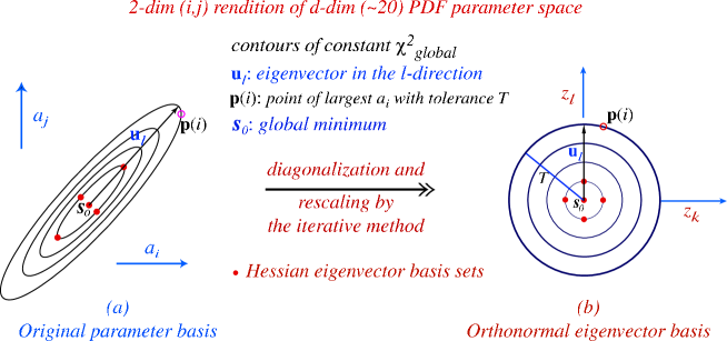
Figure 1: Representation of diagonalization of Hessian matrix.

In practice it is problematic due to extreme variations in $\Delta\chi^{2}$ in different directions in parameter space. This is solved by finding and rescaling eigenvectors of $H$ leading to the diagonal form

$$\Delta\chi^{2}=\sum_{i}z_{i}^{2}.$$ (18)

The method has been implemented by CTEQ [28, 27, 3]. The uncertainty on a physical quantity is

$$(\Delta F)^{2}=\sum_{i}\bigl{(}F(S_{i}^{(+)})-F(S_{i}^{(-)})\bigr{)}^{2},$$ (19)

where $S_{i}^{(+)}$ and $S_{i}^{(-)}$ are PDF sets displaced along eigenvector directions by the given $\Delta\chi^{2}$. There is uncertainty in choosing the “correct” $\Delta\chi^{2}$ (in principle one unit) given the complications of a full global fit. CTEQ choose $\Delta\chi^{2}\sim 100$ [26]. A discussion of this problem is found in [29].

Figure 2: Results of CTEQ Hessian approach for gluon uncertainty.

2.2 The Offset Method.

In this case the best fit is obtained by minimizing

$$\chi^{2}=\sum_{i=1}^{N}\biggl{(}\frac{(D_{i}-f_{i}(a,s))}{\sigma_{i,unc}}\biggr{)}^{2},$$ (20)

i.e. the best fit and parameters $a_{0}$ are obtained by considering only uncorrelated errors. This forces the theory to be close to unshifted data. The quality of the fit is then estimated by adding errors in quadrature. The systematic errors on the $a_{i}$ are determined by letting each $s_{k}=\pm 1$ and adding the deviations in quadrature. In practice one calculates 2 Hessian matrices

$$M_{ij}=\frac{\partial^{2}\chi^{2}}{\partial a_{i}\partial a_{j}}\qquad V_{ij}=\frac{\partial^{2}\chi^{2}}{\partial a_{i}\partial s_{j}},$$ (21)

and defines covariance matrices

$$C_{stat}=M^{-1}\qquad C_{sys}=M^{-1}VV^{T}M^{-1}\qquad C_{tot}=C_{stat}+C_{sys}.$$ (22)

to achieve the same result. This was used in early H1 fits [30] and by ZEUS. A discussion and presentation of this method and of ZEUS results can be found in [31]. The offset method leads to a bigger uncertainty than the Hessian method for the same $\Delta\chi^{2}$ [32].

2.3 Statistical Approach[8]

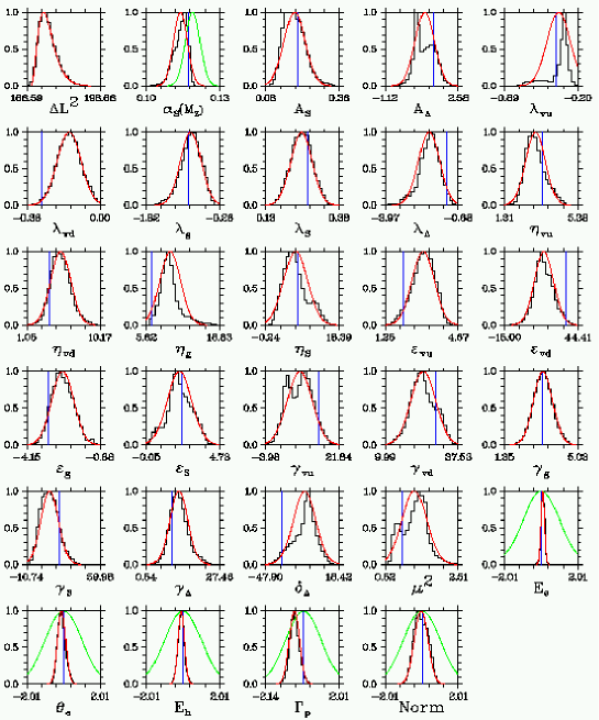
Figure 3: One set of parton parameters obtained from [8]. The red curve is the Gaussian approximation and the blue line the MRST value. The green curve for $\alpha_{S}$ is the LEP result.

In this one constructs an ensemble of distributions labelled by ${\cal F}$ each with probability $P(\{{\cal F}\})$. The mean $\mu_{O}$ and deviation $\sigma_{O}$ of observable $O$ are then given by

$$\mu_{O}=\sum_{\{{\cal F}\}}O(\{{\cal F}\})P(\{{\cal F}\}),\quad\sigma_{O}^{2}=\sum_{\{{\cal F}\}}(O(\{{\cal F}\})-\mu_{O})^{2}P(\{{\cal F}\}).$$ (23)

While this is statistically correct, and does not rely on the approximation of linear propagation of errors in calculating observables, it is inefficient. In practice, one generates $N_{pdf}$ different distributions with unit weight but distributed according to $P(\{{\cal F}\})$ where $N_{pdf}$ can be made as small as 100. Then

$$\mu_{O}=\frac{1}{N_{pdf}}\sum_{1}^{N_{pdf}}O(\{{\cal F}\}),\quad\sigma_{O}^{2}=\frac{1}{N_{pdf}}\sum_{1}^{N_{pdf}}(O(\{{\cal F}\})-\mu_{O})^{2}.$$ (24)

One can incorporate full information about measurements and their error correlations in the calculation of $P(\{{\cal F}\})$.

Currently the authors of [8] use only proton DIS data sets in order to avoid complicated uncertainty issues such as shadowing effects for nuclear targets. Using strict confidence limits they find it difficult to obtain consistency between many different DIS experiments. Also the lack of important data sets leads to “unusual” values for some parameters, which illustrates the importance of using a wide variety of data. However, fig. 3 shows that indeed the Gaussian approximation is often not good, and shows potential complications for the more simplistic approaches. This is a very attractive but ambitious large-scale project with a lot of work still to be done.

2.4 Lagrange Multiplier

One can look at the uncertainty on a given physical quantity using the Lagrange Multiplier method, first suggested by CTEQ [26] and also used by MRST [33, 34]. One performs the global fit while constraining the value of some physical quantity, i.e. minimizing

$$\Psi(\lambda,a)=\chi^{2}_{global}(a)+\lambda F(a)$$ (25)

for various values of $\lambda$. This gives the set of best fits for particular values of the parameter $F(a)$ without relying on the Gaussian approximation for $\Delta\chi^{2}$. A useful example is the $W$ cross-section at Tevatron which is illustrated in fig. 4. The uncertainty in a quantity is determined by deciding an allowed value of $\Delta\chi^{2}$.

Figure 4: Variation of $\sigma_{W}$ with total $\chi^{2}$ for the CTEQ fit.

CTEQ use $\Delta\chi^{2}=100$ (same as for the Hessian approach). They obtain for $\alpha_{S}=0.118$ [3]

$$\Delta\sigma_{W}(\rm LHC) \approx \pm 4\%\quad\Delta\sigma_{W}({\rm Tev})\approx\pm 5\%$$

$$\Delta\sigma_{H}({\rm LHC}) \approx \pm 5\%.$$ (26)

The procedure is also used by MRST for a wider range of data, and using $\Delta\chi^{2}\sim 50$. They find that for $\alpha_{S}=0.119$ [34]

$$\Delta\sigma_{W}(\rm Tev) \approx \pm 1.2\%\quad\Delta\sigma_{W}({\rm LHC})\approx\pm 2\%$$

$$\Delta\sigma_{H}(\rm Tev) \approx \pm 4\%\quad\Delta\sigma_{H}({\rm LHC})\approx\pm 2\%.$$ (27)

If $\alpha_{S}$ also varies, $\Delta\sigma_{W}$ is quite stable but $\Delta\sigma_{H}$ almost doubles. The $\chi^{2}$ profile is shown in fig. 5. One can repeat for other processes, e.g. HERA charged current data are sensitive to very high $x$ quarks, the Tevatron jet data is sensitive to high $x$ gluon etc..

Overall one concludes that the uncertainty due to experimental errors is rather small, however they are dealt with. It only exceeds a few $\%$ for quantities related to the high $x$ gluon or very high $x$ quarks. However, there are other sources of error.

Figure 5: $\Delta\chi^{2}$-plot for $W$ and Higgs production at the Tevatron and LHC with $\alpha_{S}$ free. Contours show increments of 50 in $\Delta\chi^{2}$.

3 Other Errors.

To obtain a complete estimate of errors, one also needs to consider the effect of the assumptions made during the fit. These include the cuts made on the data, the data sets fit, the parameterization for the input sets, the form of strange sea, the assumption of no isospin violation, etc.. It is known that many of these can be as important as the experimental errors on data used (or even more so). A more systematic study is needed.

It is also vital to consider sources of theoretical error. These include higher twist at low $Q^{2}$ and higher orders in $\alpha_{S}$. The latter are due not only to NNLO corrections, but also to enhancements at large and small $x$ because of terms of the form $\alpha_{s}^{n}\ln^{n-1}(1/x)$ and $\alpha_{s}^{n}\ln^{2n-1}(1-x)$ in the perturbative expansion. This means that renormalization and factorization scale variation are not a reliable way of estimating higher order effects, e.g., at small $x$

$$P^{1}_{qg}\sim\alpha_{S}(\mu^{2})\qquad\qquad P^{2}_{qg}\sim\frac{\alpha_{s}(\mu^{2})}{x}$$ (28)

whereas

$$P^{n}_{qg}\sim\frac{\alpha_{S}^{n}(\mu^{2})\ln^{n-2}(1/x)}{x}.$$ (29)

and scale variations of $P^{1}_{qg},P^{2}_{qg}$ never give an indication of these terms. Hence, in order to investigate the

true theoretical error we must consider some way of performing correct large and small $x$ resummations, and/or use what we already know about NNLO. The latter approach implies that some quantities may acquire large higher order corrections [35].

Alternatively, one can use the empirical approach of investigating in detail the effect of cuts on data. In order to investigate the real quality of the fits and the regions with potential problems we try changing $W^{2}_{cut}$, $Q^{2}_{cut}$ and $x_{cut}$, re-fitting and seeing if the fit to the remaining data improves and/or the input parameters change dramatically [36]. (Similar to a previous suggestion in terms of data sets rather than region of parameter space [37].) This is continued until the fit quality and the partons stabilize.

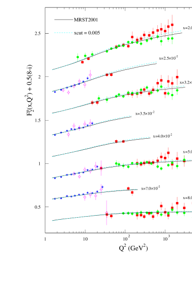
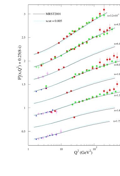
Figure 6: Comparison of MRST(2001) and a fit with $x_{cut}=0.005$.

For $W^{2}_{cut}$ raising from $12.5{\rm GeV}^{2}$ has no effect. Raising $Q^{2}_{cut}$ from $2{\rm GeV}^{2}$ there is a slow continuous improvement for higher $Q^{2}$ up to $>12{\rm GeV}^{2}$, suggesting higher order corrections may be important. The small $x$ gluon decreases slightly as does $\alpha_{S}(M_{Z}^{2})$ as $Q^{2}_{cut}$ is raised. The predictions for most quantities remain quite stable. Raising $x_{cut}$ from $0$ to $0.005$ leads to continuous improvement - $\Delta\chi^{2}=51$ for the data surviving the cut. The improvement in the fit to structure function data is shown in fig. 6, and the fit to Tevatron jet data also improves. For $x_{cut}=0.005$ there is much reduced tension between different data sets. The small $x$ gluon (outside the range of the fit) decreases significantly, allowing it to increase for higher $x$, facilitating the improved fit. $\alpha_{S}(M_{Z}^{2})$ falls slightly to $0.118$. This result suggests that higher order corrections with large $\ln(1/x)$ terms could be significant below $x=0.005$. With $x_{cut}=0.005$ predictions for Tevatron cross-sections are still possible and there is a large change compared to the default fit, as seen in fig. 7. The new prediction is well outside the limit set by experimental errors, suggesting that the theory error may easily be dominant for these quantities.

Figure 7: $\Delta\chi^{2}$-plot for $W$ and Higgs production at the Tevatron with $\alpha_{S}$ free, along with predictions for fits with different $x_{cut}$.

4 Conclusions

One can perform global fits to data over a wide range of parameter space determining the partons very precisely. The fit quality is generally good, but there are some slight worries. There are various ways of looking at the uncertainties on partons due to errors on the data. Although there has been much progress recently, there is no universally preferred approach, each having strengths and weaknesses. The errors on partons and related quantities from this source are rather small, i.e. $\sim 1-5\%$.

However, the uncertainties from input assumptions e.g. cuts on data, parameterizations etc., are comparable and possibly larger. Also, the errors from higher orders corrections are potentially large, particularly in some regions of parameter space, and due to correlations between partons in different regions of phase space these feed into all regions (e.g. the small $x$ gluon influences large $x$ gluon). For some/many processes theory is probably the dominant source of uncertainty at present. Systematic study of assumption/theory errors is needed as well as studies of uncertainties due to errors. This is much harder, and is just beginning.

Acknowledgements

I would like to thank the workshop organizers L.Lyons, M. Whalley and W.J. Stirling for inviting to present this talk.

References

- [1] M. Glück, E. Reya and A. Vogt, Eur. Phys. J. C5 (1998) 461.
- [2] A.D. Martin, R.G. Roberts, W.J. Stirling and R.S. Thorne, Eur. Phys. J. C23 (2002) 73.
- [3] CTEQ Collaboration: J. Pumplin et al., hep-ph/0201195.
-
[4]
H1 Collab: C. Adloff et al, Eur. Phys. J.
C21 (2001) 33;
B. Reisert, Presented at DIS2002, Krakow, Poland, May 2002. - [5] S. I. Alekhin, Phys. Rev. D63 (2001) 094022.
- [6] M. Botje, Eur. Phys. J. C14 (2000) 285.
-
[7]
E. Tassi, Presented at DIS2002, Krakow, Poland,
May 2002;
ZEUS Collab: S. Chekanov et al, in preparation. -
[8]
W. T. Giele and S. Keller, Phys. Rev. D58 (1998) 094023;
W. T. Giele, S. Keller and D. A. Kosower, hep-ph/0104052. -
[9]
H1 Collaboration: C. Adloff et al., Eur. Phys. J.
C13 (2000) 609;
H1 Collaboration: C. Adloff et al., Eur. Phys. J. C19 (2001) 269;
H1 Collaboration: C. Adloff et al., Eur. Phys. J. C21 (2001) 33. - [10] ZEUS Collaboration: S. Chekanov et al., Eur. Phys. J. C21 (2001) 443.
- [11] M.R. Adams et al., Phys. Rev. D54 (1996) 3006.
-
[12]
BCDMS Collaboration: A.C. Benvenuti et al., Phys.
Lett. B223 (1989) 485;
BCDMS Collaboration: A.C. Benvenuti et al., Phys. Lett. B236 (1989) 592. - [13] L.W. Whitlow et al., Phys. Lett. B282 (1992) 475, L.W. Whitlow, preprint SLAC-357 (1990).
- [14] NMC Collaboration: M. Arneodo et al., Nucl. Phys. B483 (1997) 3; Nucl. Phys. B487 (1997) 3.
-
[15]
CCFR Collaboration: U.K. Yang et al., Phys. Rev.
Lett. 86 (2001) 2742;
CCFR Collaboration: W.G. Seligman et al., Phys. Rev. Lett. 79 (1997) 1213. - [16] ZEUS Collaboration: J. Breitweg et al., Eur. Phys. J. C12 (2000) 35.
- [17] H1 Collaboration: C. Adloff et al., Phys. Lett. B528 (2002) 199.
- [18] E605 Collaboration: G. Moreno et al., Phys. Rev. D43 (1991) 2815.
- [19] E866 Collaboration: R.S. Towell et al., Phys. Rev. D64 (2001) 052002.
- [20] CDF Collaboration: F. Abe et al., Phys. Rev. Lett. 81 (1998) 5744.
- [21] D0 Collaboration: B. Abbott et al., Phys. Rev. Lett. 86 (2001) 1707.
- [22] CDF Collaboration: T. Affolder et al., Phys. Rev. D64 (2001) 032001.
- [23] CCFR collaboration: A.O. Bazarko et al., Z. Phys. C65 (1995) 189.
- [24] NuTeV Collaboration: M. Goncharov et al., hep-ex/0102049.
- [25] J. Blümlein and H. Böttcher, hep-ph/0203155.
- [26] D. Stump et al, Phys. Rev. D65 (2002) 014012.
- [27] J. Pumplin et al, Phys. Rev. D65 (2002) 014013.
- [28] J. Pumplin et al, Phys. Rev. D65 (2002) 014011.
- [29] R.S. Thorne et al, these proceedings.
- [30] C. Pascaud and F. Zomer 1995 Preprint LAL-95-05.
- [31] A. M. Cooper-Sarkar, these proceedings hep-ph/0205153.
- [32] S. I. Alekhin, hep-ex/0005042.
- [33] R. S. Thorne et al., hep-ph/0106075, to appear in proceedings of DIS01, Bologna April 2001.
- [34] A. D. Martin et al., in preparation.
- [35] A.D. Martin, R.G. Roberts, W.J. Stirling and R.S. Thorne, Phys. Lett. B531 (2002) 216.
- [36] A. D. Martin et al., in preparation.
- [37] J. C. Collins and J. Pumplin, hep-ph/0105207.