Questions on Uncertainties in Parton Distributions

Abstract

A discussion is presented of the manner in which uncertainties in parton distributions and related quantities are determined. One of the central problems is the criteria used to judge what variation of the parameters describing a set of partons is acceptable within the context of a global fit. Various ways of addressing this question are outlined.

1 Introduction

The procedure of determining parton distributions by so-called global fits to data, mainly structure functions, is long established [1]-[9]. However, it is a rather more recent development to try to determine the errors on these distributions at the same time. This has come about for a number of reasons. Firstly, the sheer amount of data (full references in [10]) sensitive to various parton distributions, and the precision of this data, has become such that an accurate determination of all parton distributions is possible (with some problems only in difficult to reach regions of phase space, e.g. $x$ very near to 1). Secondly, the understanding of the experimental errors on this data has reached a new level of sophistication, with the systematic errors being understood far better in terms of their separate sources and correlations. Lastly, the theoretical understanding at NLO in $\alpha_{S}$ has improved so that subtleties due to e.g. heavy quarks are now understood.

There are many issues in the determination of errors on parton distributions, and a discussion of these may be found in [10]. However, one of the main outstanding problems, and the focus of a discussion session at this meeting, is the manner in which one determines precisely the size of the errors.

2 Quality of fit

The quality of the fit to a set of data is generally presented in terms of the $\chi^{2}$. Taking fully into account the correlated systematic errors this may be calculated by the covariance matrix method, i.e. the covariance matrix is constructed as

$$C_{ij}=\delta_{ij}\sigma_{i,stat}^{2}+\sum_{k=1}^{n}\rho^{k}_{ij}\sigma_{k,i}\sigma_{k,j},$$ (1)

where $k$ runs over each source of correlated systematic error and $\rho^{k}_{ij}$ are the correlation coefficients. The $\chi^{2}$ is then defined by

$$\chi^{2}=\sum_{i=1}^{N}\sum_{j=1}^{N}(D_{i}-T_{i}(a))C^{-1}_{ij}(D_{j}-T_{j}(a)),$$ (2)

where $N$ is the number of data points, $D_{i}$ is the measurement and $T_{i}(a)$ is the theoretical prediction depending on parton input parameters $a$. Alternatively, one can incorporate the systematic errors into the theory prediction

$$f_{i}(a,s)=T_{i}(a)+\sum_{k=1}^{n}s_{k}\Delta_{ik},$$ (3)

where $\Delta_{ik}$ is the one-sigma correlated error for point $i$ from source $k$. The $\chi^{2}$ is then defined by

$$\chi^{2}=\sum_{i=1}^{N}\biggl{(}\frac{D_{i}-f_{i}(a,s)}{\sigma_{i,unc}}\biggr{)}^{2}+\sum_{k=1}^{n}s_{k}^{2},$$ (4)

where the second term constrains the values of $s_{k}$, assuming that the correlated systematic errors are Gaussian distributed. This is identical to the correlation matrix definition of $\chi^{2}$ if the errors are small. In many cases the statistical and systematic errors are simply added in quadrature, either for simplicity, because this has much the same result as the above procedures, or due to lack of information on the correlations of systematic errors. (The sophisticated treatment is found to be essential for Tevatron jets where correlated systematic errors dominate.)

All groups performing global fits use some combination of the above ways to calculate $\chi^{2}$, and minimizing with respect to the defined $\chi^{2}$ completely determines the parton distributions. In general, the quality of the total fit is reasonably good, e.g. for CTEQ6 one obtains $\chi^{2}/d.o.f.=1954/1811$ and for MRST2001 $\chi^{2}/d.o.f.=2328/2097$.

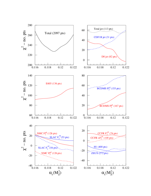
Figure 1: The quality of the fit to the individual data sets included in the global analysis by MRST, shown together with the grand total $\chi^{2}$, as a function of $\alpha_{S}(M_{Z}^{2})$

In principle, the one-$\sigma$ error on some parameter in the fit, e.g. the value of $\alpha_{S}(M_{Z}^{2})$ or one of the parameters describing the input parton distributions, can be determined by allowing the value of $\chi^{2}$ to vary one unit from its minimum. In practice, this results in unrealistically small errors. This is shown in Fig. 1, which shows the variation of the $\chi^{2}$ with $\alpha_{S}(M_{Z}^{2})$ for the total fit, and for individual sets within the global fit for the MRST partons.

It is also demonstrated in an alternative manner in Fig. 2, where for the CTEQ6 fit the extraction of $\alpha_{S}(M_{Z}^{2})$ obtained by allowing $\chi^{2}$ to increase by one unit for each data set within the fit is presented [11]. Clearly the size of the errors and the scatter of the points are unrealistic.

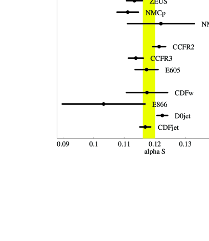
Figure 2: Values of $\alpha_{S}(M_{Z}^{2})$ obtained by CTEQ from the quality of fit to individual data sets within the global fit.

This failure of the $\Delta\chi^{2}=1$ rule may have various sources. Firstly, it is clear from examination that not all of the data sets are consistent with each other, i.e. the errors have been underestimated in some manner. Thus fitting the data simultaneously leads to a certain degree of inconsistency. One could keep only those sets which are clearly consistent with each other (within the context of NLO QCD) [9]. However, this leads to a severe restriction in the amount of data used, and the partons in some regions would lose important constraints. (Due to the correlation between different regions of $x$ via sum rules and because evolution equations for partons involve convolutions over a range of $x$, problems in one range of $x$ impact on the partons over the whole range.) A second problem is that certain assumptions have to be made when performing a global fit. These include the cuts made on data, data sets included in the fit, the parameterization for input parton sets, the form of strange sea, the precise heavy flavour prescription, the definition of the NLO strong coupling constant, the starting scale of evolution etc. Many of these can lead to variations considerably greater than those obtained from $\Delta\chi^{2}=1$. Finally, we do not have a perfect theory – NLO-in-$\alpha_{S}$ QCD has many corrections. Obviously there are higher orders (NNLO), which are not that small in themselves in QCD, but there are other problems. In particular at large and small $x$ there are large logarithms associated with higher orders, i.e. at small $x$ there are terms of the type $\alpha_{s}^{n}\ln^{n-1}(1/x)$, and at large $x$ terms like $\alpha_{s}^{n}\ln^{2n-1}(1-x)$. These are not fully understood. Also at low $Q^{2}$ there are higher twist, i.e. ${\cal O}(1/Q^{2})$ corrections that are again not well understood. Hence, in fitting data one parameter may be artificially well constrained at some incorrect value in some region of parameter space by the necessity to account for missing corrections to the theory. This can then influence other regions in the manner explained above, e.g. an artificially large gluon in one range of $x$ can lead to it being too small in other regions because of the momentum sum rule constraint.

This has led to various methods to determine errors by allowing a wider variation than the canonical $\Delta\chi^{2}=1$. CTEQ actually allow $\Delta\chi^{2}=100$ by various considerations, including error limits of individual experiments [12]. An example is the determination of $\alpha_{S}(M_{Z}^{2})$ as shown in Fig. 3, where the error bars give the $90\%$ confidence limit for each experiment (the size of which varies considerably between data sets), and the two lines give the band of $\alpha_{S}(M_{Z}^{2})$ allowed by $\Delta\chi^{2}=100$ for the global fit [11]. Arguably this is too conservative, and CTEQ regard it as more than a one-$\sigma$ error. MRST use $\Delta\chi^{2}=20$ as an approximate one-$\sigma$ error instead, based on the essentially subjective criterion of judging when the fit is going uncomfortably wrong in some region [2].

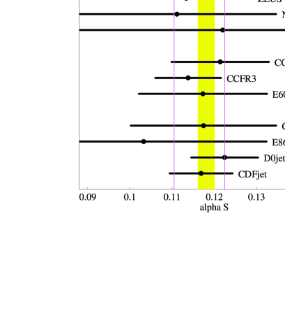
Figure 3: Allowed value of $\alpha_{S}(M_{Z}^{2})$ obtained by CTEQ from the quality of fit to individual data sets within global fit.

A more precisely defined method is to use an alternative formulation for $\chi^{2}$. In the offset method the fit is obtained by minimizing

$$\chi^{2}=\sum_{i=1}^{N}\biggl{(}\frac{(D_{i}-f_{i}(a,s))}{\sigma_{i,unc}}\biggr{)}^{2},$$ (5)

i.e. the best fit and parameters $a_{0}$ are obtained from only uncorrelated errors. The quality of the fit can then be estimated by adding errors in quadrature. The systematic errors on $a_{i}$ are determined by letting each $s_{k}=\pm 1$ and adding the deviations in quadrature. This is essentially the same as, and in practice achieved by calculating 2 Hessian matrices

$$M_{ij}=\frac{\partial^{2}\chi^{2}}{\partial a_{i}\partial a_{j}}\qquad V_{ij}=\frac{\partial^{2}\chi^{2}}{\partial a_{i}\partial s_{j}},$$ (6)

and defining covariance matrices

$$C_{stat}=M^{-1}\qquad C_{sys}=M^{-1}VV^{T}M^{-1}\qquad C_{tot}=C_{stat}+C_{sys}.$$ (7)

This method was used in early H1 fits [13] and in ZEUS fits [6, 7]. Much the same method is used for polarized data in [8], as far as the information on correlated errors allows. Strictly speaking, the method is not optimum, and it leads to a much bigger uncertainty than the standard method for $\Delta\chi^{2}=1$ [14]. However, it may be suitable in practice [7], and ZEUS estimate the same results could be obtained using the standard method and $\Delta\chi^{2}=50$.

The results of the various approaches may be summarized in a selection of the extracted values of $\alpha_{S}(M_{Z}^{2})$ below [15].

$$\hbox{CTEQ6}\quad(\Delta\chi^{2}=100)\quad\alpha_{S}(M_{Z}^{2}) = 0.1165\pm 0.0065$$

$$\hbox{ZEUS}\quad(\Delta\chi^{2}_{eff}=50)\quad\alpha_{S}(M_{Z}^{2}) = 0.1166\pm 0.0008(\hbox{uncor})\pm 0.0032(\hbox{corr})$$

$$\pm 0.0036(\hbox{norm})\pm 0.0018(\hbox{model})$$

$$\hbox{MRST}\quad(\Delta\chi^{2}=20)\quad\alpha_{S}(M_{Z}^{2}) = 0.119\pm 0.002(\hbox{exp})\pm 0.003(\hbox{theory})$$

$$\hbox{H1}\quad(\Delta\chi^{2}=1)\quad\alpha_{S}(M_{Z}^{2}) = 0.115\pm 0.0017(\hbox{exp})\pm 0.005(\hbox{theory})$$ (8)

The values obtained are consistent, and the errors not too dissimilar given the wide variation in $\Delta\chi^{2}$ used. This is largely because each group has chosen a method which gives a reasonable and believable error. H1 actually use the standard definition, obtaining a small error, but are only able to do this because they use a much smaller data set than the other groups, i.e. their own data plus some BCDMS data which are fully consistent. If MRST and CTEQ were to use the same approach their error would be tiny (and their extracted value of $\alpha_{S}(M_{Z}^{2})$ some standard deviations away from that of H1, e.g. MRST2001 would obtain $\alpha_{S}(M_{Z}^{2})=0.1192\pm 0.0005$).

3 Conclusions

In determining errors for and from parton distributions one encounters a dilemma. One could fit to a relatively small subset of the available data with a very conservative set of cuts so that data are self consistent and theory is truly reliable. However, this would lead to a poor determination of partons in certain regions and would give no idea how well the theory is working overall. Alternatively, one can try to constrain the partons in as wide a region of parameter space as possible, accepting that the standard rules for error determination will break down. The way in which one can obtain sensible estimates of the real errors in the latter case is a subject very much open for discussion.

Acknowledgements

We would like to thank some of our colleagues not at the discussion, A.D. Martin, J. Pumplin, R.G. Roberts and W.K. Tung for useful comments and the workshop organizers L.Lyons and M. Whalley.

References

- [1] M. Glück, E. Reya and A. Vogt, Eur. Phys. J. C5 (1998) 461.
- [2] A.D. Martin, R.G. Roberts, W.J. Stirling and R.S. Thorne, Eur. Phys. J. C23 (2002) 73.
- [3] CTEQ Collaboration: J. Pumplin et al., hep-ph/0201195.
-
[4]
H1 Collab: C. Adloff et al., Eur. Phys. J.
C21 (2001) 33;
B. Reisert, presented at DIS2002, Krakow, Poland, May 2002. - [5] S. I. Alekhin, Phys. Rev. D63 (2001) 094022.
- [6] M. Botje, Eur. Phys. J. C14 (2000) 285.
-
[7]
A. M. Cooper-Sarkar, these proceeding hep-ph/0205153;
ZEUS Collab: S. Chekanov et al., in preparation. - [8] J. Blümlein and H. Böttcher, hep-ph/0203155.
-
[9]
W. T. Giele and S. Keller, Phys. Rev. D58 (1998) 094023;
W. T. Giele, S. Keller and D. A. Kosower, hep-ph/0104052. - [10] R.S. Thorne, these proceedings.
- [11] W.K. Tung, talk presented at DIS2002, Krakow, Poland, May 2002.
- [12] D. Stump et al., Phys. Rev. D65 (2002) 014012.
- [13] C. Pascaud and F. Zomer 1995 Preprint LAL-95-05.
- [14] S. I. Alekhin, hep-ex/0005042.
- [15] A. M. Cooper-Sarkar, V. Shekelyan and R. S. Thorne, Structure Functions summary talk presented at DIS2002, Krakow (May 2002).