An Overview of the Sources for Electroweak Baryogenesis^∗

Abstract

After a short review of electroweak scale baryogenesis, we consider the dynamics of chiral fermions coupled to a complex scalar field through the standard Yukawa interaction term at a strongly first order electroweak phase transition. By performing a systematic gradient expansion we can use this simple model to study electroweak scale baryogenesis. We show that the dominant sources for electroweak baryogenesis appear at linear order in the Planck constant $\hbar$. We provide explicit expressions for the sources both in the flow term and in the collision term of the relevant kinetic Boltzmann equation. Finally, we indicate how the kinetic equation sources appear in the fluid transport equations used for baryogenesis calculations.

^∗ Presented at the ‘8th Adriatic meeting on particle physics in the new millennium’ (Dubrovnik, Croatia, 4 - 14 September 2001) [Preprint: HD-THEP-02-18]

1 Introduction

The necessary requirements on dynamical baryogenesis at an epoch of the early Universe are provided by the following Sakharov conditions:

• baryon number (B) violation

• charge (C) and charge-parity (CP) violation

• departure from thermal and kinetic equilibrium

The Sakharov conditions may be realised at the electroweak transition [1], provided the transition is strongly first order. Namely, C and CP violation are realised in the standard model (SM) for example through the Cabibbo-Kobayashi-Maskawa (CKM) matrix of quarks. B violation is mediated through the Adler-Bell-Jackiw (ABJ) anomaly. At high temperatures the ABJ anomaly is manifest via the unsuppressed sphaleron transitions, and may be responsible for the observed baryon asymmetry today, which is usually expressed as the baryon-to-entropy ratio:

$$\frac{n_{B}}{s}=3-7\times 10^{-11}.$$ (1)

This is obtained both as a nucleosynthesis constraint and from recent cosmic microwave background observations.

The standard model (SM) of elementary particles and interactions cannot alone be responsible for the observed matter-antimatter asymmetry (1), primarily because the LEP bound on the Higgs mass $m_{H}\ga 112$ GeV is inconsistent with the requirement that the transition be strongly first order. A strongly first order transition is namely required in order for the baryons produced in the symmetric phase not be washed-out by the sphaleron transitions in the Higgs (‘broken’) phase. And this is so provided the transition is strong enough. This is usually expressed as the requirement $\Delta\phi\ga 1.1T$ on the jump in the Higgs expectation value $\phi$ of the phase transition [2].

Supersymmetric extensions of the Standard Model on the other hand may result in a strongly first order transition. For example, in the Minimal supersymmetric standard model the sphaleron bound can be satisfied provided the stop and the lightest Higgs particles are not too heavy, $m_{\tilde{t}}\sim 120$ GeV and $m_{H}\la 120$ GeV [3].

An efficient mechanism for baryon production at the electroweak phase transition is the charge transport mechanism [4], which works as follows. At a first order transition, when the Universe supercools, the bubbles of the Higgs phase nucleate and grow. In presence of a CP-violating condensate at the bubble interface, as a consequence of collisions of chiral fermions with scalar particles in presence of a scalar field condensate, CP-violating currents are created and transported into the symmetric phase, where they bias baryon number production. The baryons thus produced are transported back into the Higgs phase where they are frozen-in. The main unsolved problem of electroweak baryogenesis is systematic computation of the relevant CP-violating currents generated at the bubble interface. Here we shall reformulate this problem in terms of calculating CP-violating sources in the kinetic Boltzmann equations for fermions.

Figure 1: The tree level interactions of fermions with the scalar field condensate which, when expanded in gradients, lead to the CP-violating semiclassical force in the kinetic Boltzmann equation.

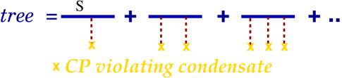
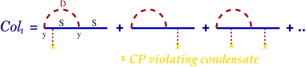
The techniques we report here are relevant for calculation of sources in the limit of thick phase boundaries and a weak coupling to the Higgs condensate. In this case one can show that, to linear order in the Planck constant $\hbar$, the quasiparticle picture for fermions survives [5, 6]. In presence of a CP-violating condensate there are two types of sources: the semiclassical force in the flow term of the kinetic Boltzmann equation, and the collisional sources. The semiclassical force was originally introduced for baryogenesis in two-Higgs doublet models in [7], and subsequently adapted to the chargino baryogenesis in the Minimal Supersymmetric Standard Model (MSSM) in [8]. The semiclassical force corresponds to tree level interactions with the condensate shown in figure 1 and it is universal in that its form is independent on interactions. The collisional sources on the other hand arise when fermions in the loop diagrams interact with scalar condensates. In figure 2 we show typical CP-violating one-loop contributions to the collisional source. This source arises from one-loop diagrams in which fermions interact with a CP-violating scalar condensate. When viewed in the kinetic Boltzmann equation, these processes correspond to tree-level interactions in which fermions absorb or emit scalar particles, whilst interacting in a CP-violating manner with the scalar condensate. The precise form of the collisional source depends on the form of the interaction. In the following sections we discuss how one can study the CP-violating collisional sources induced by a typical Yukawa interaction term.

Figure 2: The one-loop fermion-scalar diagrams, where interactions of fermions with the scalar field condensate are explicitly shown. The condensate interactions, when expanded in gradients, result in a CP-violating collisional source in the kinetic Boltzmann equation. Upon projecting (or ‘cutting’) the loop propagators on-shell one obtains the CP-violating scalar particle absorption and emission processes.

2 Kinetic equations

Here we work in the simple model of chiral fermions coupled to a complex scalar field via the Yukawa interaction with the Lagrangian of the form [5, 6]

$${\cal L}=i\bar{\psi}{\mathbin{\partial\mkern-10.5mu\big{/}}}\psi-\bar{\psi}_{L}m\psi_{R}-\bar{\psi}_{R}m^{*}\psi_{L}+{\cal L}_{\rm Yu},$$ (2)

where ${\cal L}_{\rm Yu}$ denotes the Yukawa interaction term

$${\cal L}_{\rm Yu}=-y\phi\bar{\psi}_{L}\psi_{R}-y\phi^{*}\bar{\psi}_{R}\psi_{L},$$ (3)

and $m$ is a complex, spatially varying mass term

$$m(u)\equiv y^{\prime}\Phi_{0}=m_{R}(u)+im_{I}(u)=|m(u)|\mbox{e}^{i\theta(u)}.$$ (4)

Such a mass term arises naturally from an interaction with a scalar field condensate $\Phi_{0}=\langle\hat{\Phi}(u)\rangle$. This situation is realised for example by the Higgs field condensate of a first order electroweak phase transition in supersymmetric models. When $\phi$ in (3) is the Higgs field the coupling constants $y$ and $y^{\prime}$ coincide. Our considerations are however not limited to this case.

The dynamics of quantum fields can be studied by considering the equations of motion arising from the two-particle irreducible (2PI) effective action [9] in the Schwinger-Keldysh closed-time-path formalism [10, 11]. This formalism is suitable for studying the dynamics of the non-equilibrium fermionic and bosonic two-point functions

$$iS_{\alpha\beta}(u,v) = \langle\Omega|T_{{\cal C}}\big{[}\psi_{\alpha}(u)\bar{\psi}_{\beta}(v)\big{]}|\Omega\rangle$$ (5)

$$i\Delta(u,v) = \langle\Omega|T_{{\cal C}}\big{[}\phi(u){\phi}^{\dagger}(v)\big{]}|\Omega\rangle,$$ (6)

where $|\Omega\rangle$ is the physical state, and the time ordering $T_{{\cal C}}$ is along the Schwinger contour shown in figure 3. For our purposes it suffices to consider the limit when $t_{0}\rightarrow-\infty$. The complex path time ordering can be conveniently represented in the Keldysh component formalism. For example, for nonequilibrium dynamics of quantum fields the following Wightman propagator is relevant

$$iS^{<}(u,v)=-\langle\Omega|\bar{\psi}(v)\psi(u)|\Omega\rangle.$$ (7)

       

Figure 3: The complex time contour for the Schwinger-Keldysh nonequilibrium formalism.

For thick walls, that is for the plasma excitations whose de Broglie wavelength $\ell_{\rm dB}$ is small in comparison to the phase interface thickness $L_{w}$, it is suitable to work in the Wigner representation for the propagators, which corresponds to the Fourier transform with respect to the relative coordinate $r=u-v$, and expand in the gradients of average coordinate $x=(u+v)/2$. This then represents an expansion in powers of $\ell_{\rm dB}/L_{w}$. When written in this Wigner representation, the kinetic equations for fermions become [12]

$${\cal D}S^{<}\equiv\Big{(}\frac{i}{2}\partial\!\!\!/+k\!\!\!/-(mP_{R}-m^{*}P_{L})e^{{-\frac{i}{2}\stackrel{{\scriptstyle\leftarrow}}{{\partial}}}\cdot\;\partial_{k}}\Big{)}S^{<}={\cal C}_{\psi},$$ (8)

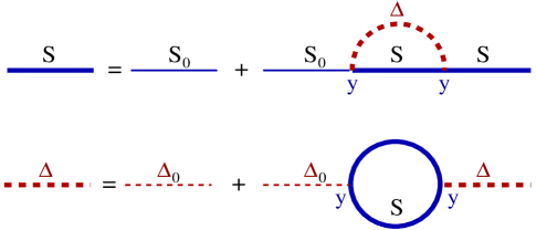
where for simplicity we neglected the contributions from self-energy corrections to the mass and the collisional broadening term [12]. When the collision term ${\cal C}_{\psi}$ is approximated at one loop, equation (8) corresponds to the nonequilibrium fermionic Schwinger-Dyson equation shown in figure 4. Since the scalar equation (also shown in figure 4) does not yield CP-violating sources at first order in gradients [5, 14], we shall not discuss it here.

Figure 4: The one-loop Schwinger-Dyson equations for the out-of-equilibrium fermionic ($S$) and scalar ($\Delta$) propagators. When projected on-shell and expanded in gradients, these equations reduce to the kinetic Boltzmann equations.

As the bubbles grow large, they tend to become more and more planar. Hence, it suffices to consider the limit of a planar phase interface, in which the mass condensate in the wall frame becomes a function of one coordinate only, $m=m(z)$. Further, we keep only the terms that contribute at order $\hbar$ to Eq. (8), which implies that we need to keep second order gradients of the mass term

$$me^{{-\frac{i}{2}\stackrel{{\scriptstyle\leftarrow}}{{\partial}}}\cdot\;\partial_{k}}=m+\frac{i}{2}m^{\prime}\partial_{k_{z}}-\frac{1}{8}m^{\prime\prime}\partial_{k_{z}}^{2}+o(\partial_{z}^{3}),$$ (9)

where $m=m(z)$, $m^{\prime}\equiv\partial_{z}m$ and $m^{\prime\prime}\equiv\partial_{z}^{2}m$. On the other hand, in the collision term ${\cal C}_{\psi}$ we need to consider terms only up to linear order in derivatives

$${\cal C}_{\psi} = {\cal C}_{\psi 0}+{\cal C}_{\psi 1}+..$$

$${\cal C}_{\psi 0} = -\frac{1}{2}\Big{(}\Sigma^{>}S^{<}-\Sigma^{<}S^{>}\Big{)}$$

$${\cal C}_{\psi 1} = -\frac{i}{4}(\partial_{z}^{(1)}\partial_{k_{z}}^{(2)}-\partial_{k_{z}}^{(1)}\partial_{z}^{(2)})\Big{(}\Sigma^{>}S^{<}-\Sigma^{<}S^{>}\Big{)},$$ (10)

where $\Sigma^{<}$ and $\Sigma^{>}$ represent the fermionic self-energies, and the derivatives $\partial_{z}^{(1)}$, $\partial_{k_{z}}^{(1)}$ ($\partial_{z}^{(2)}$, $\partial_{k_{z}}^{(2)}$) act on the first (second) factor in the parentheses.

An important observation is that, when $G=G(k_{\mu},t-\vec{x}_{\|}\cdot\vec{k}_{\|},z)$, the spin in the $z$-direction (of the interface motion)

$$S_{z}\equiv L^{-1}(\Lambda)\,\tilde{\!S}_{z}L(\Lambda)\;=\;\gamma_{\|}\Big{(}\tilde{S}_{z}-i(\vec{v}_{\|}\times\vec{\alpha})_{z}\Big{)}$$ (11)

is conserved

$$[{\cal D},S_{z}]S^{<}=0,$$ (12)

where ${\cal D}$ is the differential operator in Eq. (8), $\vec{\alpha}=\gamma^{0}\vec{\gamma}$, $\tilde{S}_{z}=\gamma^{0}\gamma^{3}\gamma^{5}$, and $\gamma_{\|}=1/(1-\vec{v}_{\|}^{2})^{1/2}$. This then implies that, without a loss of generality, the fermionic Wigner function can be written in the following block-diagonal form

$$S^{<} = \sum_{s=\pm}S_{s}^{<}$$

$$S^{<} = L(\Lambda)^{-1}\tilde{S}^{<}L(\Lambda)$$

$$-i\gamma^{0}\tilde{S}^{<}_{s} = \frac{1}{4}({\mathbf{1}}+s\sigma^{3})\otimes\rho^{a}\tilde{g}^{s}_{a},$$ (13)

where $\sigma^{3}$ and $\rho^{i}$ ($i=1,2,3$) are the Pauli matrices and $\rho^{0}={\mathbf{1}}$ is the $2\times 2$ unity matrix and $L(\Lambda)$ is the following Lorentz boost operator

$$L(\Lambda)=\frac{k_{0}+\tilde{k}_{0}-\gamma^{0}\vec{\gamma}\cdot\vec{k}_{\|}}{\sqrt{2\tilde{k}_{0}(k_{0}+\tilde{k}_{0})}},$$ (14)

with $\tilde{k}_{0}={\rm sign}(k_{0})({k_{0}^{2}-\vec{k}_{\|}^{2}})^{1/2}$. The boost $\Lambda$ corresponds to a Lorentz transformation that transforms away $\vec{k}_{\|}$.

With the decomposition (13) the trace of the antihermitean part of Eq. (8) can be written as the following algebraic constraint equation [6]

$$\left(k^{2}-|m|^{2}+\frac{s}{\tilde{k}_{0}}(|m|^{2}\theta^{\prime})\right)g^{s}_{00}=0,$$ (15)

where $g^{s}_{00}=\gamma_{\|}\tilde{g}_{0}^{s<}$ denotes the particle density on phase space $\{k_{\mu},x_{\nu}\}$. Equation (15) has a spectral solution

$$g^{s}_{00} \equiv \sum_{\pm}\frac{2\pi}{Z_{s\pm}}\,n_{s}\,\delta(k_{0}\mp\omega_{s\pm}),$$ (16)

where $\omega_{s\pm}$ denotes the dispersion relation

$$\omega_{s\pm}=\omega_{0}\mp s\frac{|m|^{2}\theta^{\prime}}{2\omega_{0}\tilde{\omega}_{0}},\qquad\qquad\omega_{0}=\sqrt{\vec{k}^{2}+|m|^{2}},\qquad\tilde{\omega}_{0}=\sqrt{\omega_{0}^{2}-\vec{k}_{\parallel}^{\,2}}$$ (17)

and $Z_{s\pm}=1\mp s|m|^{2}\theta^{\prime}/2\tilde{\omega}_{0}^{3}$. The delta functions in (16) project $n_{s}(k_{\mu},t-\vec{x}_{\|}\cdot\vec{k}_{\|},z)$ on-shell, thus yielding the distribution functions $f_{s+}$ and $f_{s-}$ for particles and antiparticles with spin $s$, respectively, defined by

$$f_{s+} \equiv n_{s}(\omega_{s+},k_{z},t-\vec{x}_{\|}\cdot\vec{k}_{\|},z)$$

$$f_{s-} \equiv 1-n_{s}(-\omega_{s-},-k_{z},t+\vec{x}_{\|}\cdot\vec{k}_{\|},z).$$ (18)

This on-shell projection proves the implicit assumption underlying the semiclassical WKB-methods, that the plasma can be described as a collection of single-particle excitations with a nontrivial space-dependent dispersion relation. In fact, the decomposition (13), Eq. (15) and the subsequent discussion imply that the physical states that correspond to the quasiparticle plasma excitations are the eigenstates of the spin operator (11).

Taking the trace of the Hermitean part of Eq. (8), integrating over the positive and negative frequencies and taking account of (16) and (18), one obtains the following on-shell kinetic equations [6]

$$\partial_{t}f_{s\pm}+\vec{v}_{\|}\cdot\nabla_{\|}f_{s\pm}+v_{s\pm}\partial_{z}f_{s\pm}+F_{s\pm}\partial_{k_{z}}f_{s\pm}={\cal C}_{\psi s\pm}[f_{s\pm}],$$ (19)

where $f_{s\pm}=f_{s\pm}(k_{\mu},z,\,t-\vec{v}_{\|}\cdot\vec{x}_{\|})$, ${\cal C}_{s\pm}[f_{s\pm}]$ is the collision term obtained by integrating (10) over the positive and negative frequencies, respectively, the quasiparticle group velocity $v_{s\pm}\equiv k_{z}/\omega_{s\pm}$ is expressed in terms of the kinetic momentum $k_{z}$ and the quasiparticle energy $\omega_{s\pm}$ (17), and the semiclassical force

$$F_{s\pm}=-\frac{{|m|^{2}}^{\,\prime}}{2\omega_{s\pm}}\pm\frac{s(|m|^{2}\theta^{\,\prime})^{\,\prime}}{2\omega_{0}\tilde{\omega}_{0}}.$$ (20)

In the stationary limit in the wall frame the distribution function simplifies to $f_{s\pm}=f_{s\pm}(k_{\mu},z,)$. When compared with the 1+1 dimensional case studied in [5] the sole, but significant, difference in the force (20) is that the CP-violating $\theta^{\prime}$-term is enhanced by the boost-factor $\gamma_{\parallel}=\omega_{0}/\tilde{\omega}_{0}$, $\tilde{\omega}_{0}=({\omega_{0}^{2}-\vec{k}_{\parallel}^{\,2}})^{1/2}$, which, when integrated over the momenta, leads to an enhancement by about a factor two in the CP-violating source from the semiclassical force.

3 Sources for baryogenesis in the fluid equations

Fluid transport equations are usually obtained by taking first two moments of the Boltzmann transport equation (19). That is, integrating Eq. (19) over the spatial momenta results in the continuity equation for the vector current, while multiplying by the velocity and integrating over the momenta yields the Euler equation. The physical content of these equations can be summarized as the particle number and fluid momentum density conservation laws for fluids, respectively. This procedure is necessarily approximate simply because the fluid equations describe only very roughly the rich momentum dependence described by the distribution functions of the Boltzmann equation (20). The fluid equations can be easily reduced to the diffusion equation which has so far being used almost exclusively for electroweak baryogenesis calculations at a first order electroweak phase transition. A useful intermediate step in derivation of the fluid equations is rewriting Eq. (19) for the CP-violating departure from equilibrium $\delta f_{si}=\delta f_{si+}-\delta f_{si-}$ as follows

$$\left(\partial_{t}+\frac{k_{z}}{\omega_{0i}}\partial_{z}-\frac{{|m_{i}|^{2}}^{\prime}}{2\omega_{0i}}\partial_{k_{z}}\right)\delta f_{si}+v_{w}\delta F_{si}(\partial_{\omega}f_{\omega})_{\omega_{0i}}$$ (21)

$$+ v_{w}F_{0i}\delta\omega_{si}\bigg{[}\Big{(}\frac{\partial_{\omega}f_{\omega}}{\omega}\Big{)}_{\omega_{0i}}-(\partial^{2}_{\omega}f_{\omega})_{\omega_{0i}}\bigg{]}={\cal C}_{\psi si},$$

where $i$ is the species (flavour) index, $f_{\omega}=1/(e^{\beta\omega}+1)$, and

$$F_{0i} = -\frac{{|m_{i}|^{2}}^{\prime}}{2\omega_{0i}}$$

$$\delta\omega_{si} = s\frac{(|m_{i}|^{2}\theta_{i})^{\prime}}{\omega_{0i}\tilde{\omega}_{0i}}$$

$$\delta F_{si} \equiv F_{si+}-F_{si-}=s\frac{(|m_{i}|^{2}\theta_{i}^{\prime})^{\prime}}{\omega_{0i}\tilde{\omega}_{0i}}$$

$${\cal C}_{\psi si} \equiv {\cal C}_{\psi si+}-{\cal C}_{\psi si-}.$$ (22)

When integrating (21) over the momenta, the flow term yields two sources in the continuity equation for the vector current. The former comes from the CP-violating spin dependent semiclassical force, and has the form

$${\cal S}^{a}_{si} = v_{w}\int\frac{d^{3}k}{(2\pi)^{3}}\delta F_{si}(\partial_{\omega}f_{\omega})_{\omega=\omega_{0i}}$$ (23)

$$= -sv_{w}\frac{(|m_{i}|^{2}\theta^{\prime}_{i})^{\prime}}{4\pi^{2}}\;{\cal J}_{a}(x_{i})$$

with $x_{i}=|m_{i}|/T$, while the latter comes from the CP-violating shift in the quasiparticle energy, and can be written as

$${\cal S}^{b}_{si} = v_{w}\int\frac{d^{3}k}{(2\pi)^{3}}F_{0i}\delta\omega_{si}\Big{[}\big{(}\partial_{\omega}f_{\omega}/\omega\big{)}_{\omega_{0i}}-(\partial^{2}_{\omega}f_{\omega})_{\omega_{0i}}\Big{]}$$ (24)

$$= sv_{w}\frac{(|m_{i}|^{2}\theta^{\prime}_{i})}{2\pi^{2}T}{|m_{i}|}^{\prime}\;{\cal J}_{b}(x_{i}).$$

Figure 5: The flow term sources (23)-(24) characterised by the integrals $x_{i}^{2}{\cal J}_{a}(x_{i})$ (red solid) and $x_{i}^{3}{\cal J}_{b}(x_{i})$ (green dashed) as a function of the rescaled mass $x_{i}=|m_{i}|/T$. The sum of the two sources (thin blue line) is also shown.

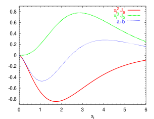
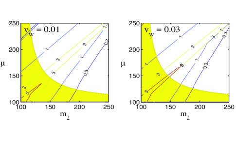
The total source is simply the sum of the two, ${\cal S}_{si}={\cal S}^{a}_{si}+{\cal S}^{b}_{si}$. To get a more quantitative understanding of these sources, in figure 5 we plot the integrals ${\cal J}_{a}$ and ${\cal J}_{b}$ in equations (23) and (24). A closer inspection of the sources ${\cal S}_{si}^{a}$ and ${\cal S}_{si}^{b}$ indicates that the total source ${\cal S}_{si}$ can be also rewritten as the sum of two sources: the source $\propto{|m_{i}|^{2}}^{\prime}\Theta_{i}^{\prime}$, characterized by $x_{i}^{2}{\cal J}_{a}+x_{i}^{3}{\cal J}_{b}$, and the source $\propto{|m_{i}|^{2}}\Theta_{i}^{\prime\prime}$, characterized by $x_{i}^{2}{\cal J}_{a}$. We note that in the spin state quasiparticle basis the flow term sources appear in the continuity equation for the vector current, while in the helicity basis, which is usually used in literature [7, 8], the flow term sources appear in the Euler equation. In figure 6 we show recent results of baryogenesis calculations of Ref. [8] based on the CP-violating contribution to the semiclassical force in the chargino sector of the Minimal Supersymmetric Standard Model (MSSM). This calculation is based on the quasiparticle picture based on helicity states. The analysis suggests that one can dynamically obtain baryon production marginally consistent with the observed value (1), provided $m_{2}\sim\mu\sim 150$ GeV and $v_{w}\sim 0.03c$.

Figure 6: The semiclassical force baryogenesis mediated by charginos of the MSSM calculated in the helicity basis. The figures show contours for the baryon-to-entropy ratio in the units of $10^{-11}$ for two wall velocities $v_{w}=0.01$ and $v_{w}=0.03$ as a function of the soft susy breaking parameters $\mu$ and $m_{2}$. A maximal CP violation in the chargino sector is assumed. The shaded (yellow) regions are ruled out by the LEP measurements. The observed baryon asymmetry is in these units $3-7$. (The figure is taken from the latter reference in [8]. )

We now turn to discussion of the collision term sources in Eqs. (19) and (21). We assume that the self-energies $\Sigma^{>,<}$ are approximated by the one-loop expressions (cf. figure 4)

$$\Sigma^{<,>}(k,x) = iy^{2}\int\frac{d^{4}k^{\prime}d^{4}k^{\prime\prime}}{(2\pi)^{8}}\,\big{[}(2\pi)^{4}\delta(k-k^{\prime}+k^{\prime\prime})P_{L}S^{<,>}(k^{\prime},x)P_{R}\Delta^{>,<}(k^{\prime\prime},x)$$ (25)

$$\qquad\qquad+(2\pi)^{4}\delta(k-k^{\prime}-k^{\prime\prime})P_{R}S^{<,>}(k^{\prime},x)P_{L}\Delta^{<,>}(k^{\prime\prime},x)\big{]},$$

where $\Delta^{<}$ and $\Delta^{>}$ denote the bosonic Wigner functions. This expression contains both the CP-violating sources and relaxation towards equilibrium. The CP-violating sources can be evaluated by approximating the Wigner functions $S^{>,<}$ and $\Delta^{>,<}$ by the equilibrium expressions accurate to first order in derivatives. The result of the investigation is as follows. There is no source contributing to the continuity equation, while the source arising in the Euler equation is of the form [12]

$$2\int_{\pm}\frac{d^{4}k}{(2\pi)^{4}}\frac{k_{z}}{\omega_{0}}{\cal C}_{\psi si} = v_{w}y^{2}\frac{s|m|^{2}\theta^{\prime}}{32\pi^{3}T}{\cal I}_{f}(|m|,m_{\phi}),$$ (26)

where the function ${\cal I}_{f}(|m|,m_{\phi})$ is plotted in figure 7. It is encouraging that the source vanishes for small values of the mass parameters, which suggests that the expansion in gradients we used here may yield the dominant sources. Note that the source is nonvanishing only in the kinematically allowed region, $m_{\phi}\geq 2|m|$. When the masses are large, $|m|,m_{\phi}\gg T$, the source is as expected Boltzmann suppressed. It would be of interest to make a detailed comparison between the sources in the flow term and those in the collision term. This is a subject of an upcoming publication.

Figure 7: The collisional source contributing to the fermionic kinetic equation at one loop for the mass ratios $m_{\phi}/|m|=2.1,2.5,3,4,10$ and 20, respectively. The source peaks for $|m|\approx 0.7T$ and $m_{\phi}\approx 4|m|$.

References

• 1. Kuzmin V. A., Rubakov V. A., Shaposhnikov M. E. (1985): On The Anomalous Electroweak Baryon Number Nonconservation In The Early Universe. Phys. Lett. B 155, 36.
• 2. Shaposhnikov M. E. (1987): Baryon Asymmetry Of The Universe In Standard Electroweak Theory. Nucl. Phys. B 287, 757.
• 3. Quiros M., Seco M. (2000): Electroweak baryogenesis in the MSSM. Nucl. Phys. Proc. Suppl.  81, 63 [arXiv:hep-ph/9903274].
• 4. Cohen A. G., Kaplan D. B., Nelson A. E. (1990): Weak Scale Baryogenesis. Phys. Lett. B 245, 561; Cohen A. G., Kaplan D. B., Nelson A. E. (1991): Baryogenesis At The Weak Phase Transition. Nucl. Phys. B 349, 727.
• 5. Kainulainen K., Prokopec T., Schmidt M. G., Weinstock S. (2001): First principle derivation of semiclassical force for electroweak baryogenesis. JHEP 0106, 031 [arXiv:hep-ph/0105295].
• 6. Kainulainen K., Prokopec T., Schmidt M. G., Weinstock S. (2002): Semiclassical force for electroweak baryogenesis: Three-dimensional derivation. arXiv:hep-ph/0202177.
• 7. Joyce M., Prokopec T., Turok N. (1996): Nonlocal electroweak baryogenesis. Part 2: The Classical regime. Phys. Rev. D 53, 2958 [arXiv:hep-ph/9410282]; Joyce M., Prokopec T., Turok N. (1995): Electroweak baryogenesis from a classical force. Phys. Rev. Lett.  75, 1695 [Erratum-ibid.  75 (1995) 3375] [arXiv:hep-ph/9408339].
• 8. Cline J. M., Kainulainen K. (2000): A new source for electroweak baryogenesis in the MSSM. Phys. Rev. Lett.  85, 5519 [hep-ph/0002272]; Cline J. M., Joyce M., Kainulainen K. (2000): Supersymmetric electroweak baryogenesis. JHEP 0007, 018 [arXiv:hep-ph/0006119]; ibid. hep-ph/0110031.
• 9. Cornwall J. M., Jackiw R., Tomboulis E. (1974): Effective Action For Composite Operators. Phys. Rev. D 10, 2428.
• 10. Schwinger J. (1961): J. Math. Phys. 2, 407; Keldysh L. V. (1964): Zh. Eksp. Teor. Fiz. 47, 1515 [Sov. Phys. JETP 20 (1965) 235].
• 11. Chou K., Su Z., Hao B., Yu L. (1985): Equilibrium And Nonequilibrium Formalisms Made Unified. Phys. Rept.  118 1; Calzetta E., Hu B. L. (1988): Nonequilibrium Quantum Fields: Closed Time Path Effective Action, Wigner Function And Boltzmann Equation. Phys. Rev. D 37, 2878.
• 12. Kainulainen K., Prokopec T., Schmidt M. G., Weinstock S. (2002): Some aspects of collisional sources for electroweak baryogenesis. arXiv:hep-ph/0201245.
• 13. Kainulainen K., Prokopec T., Schmidt M. G., Weinstock S. (2002): Quantum Boltzmann equations for electroweak baryogenesis including gauge fields. arXiv:hep-ph/0201293.
• 14. Kainulainen K., Prokopec T., Schmidt M. G., Weinstock S. (2002): in preparation.