Key words: chiral perturbation theory; $\pi\pi$ scattering; Padé approximationPACS number: 11.55.Fv, 12.39.Fe, 12.38.Cy

The chiral perturbation theory (ChPT) ([1]–[4]) is a powerful tool in studying strong interaction physics at low energies and has been extensively studied at 1–loop level [5]. The 2–loop results are also available in recent years ([6]–[9]). However, since the chiral expansion is an expansion in terms of the external momentum, the perturbation series to any finite order diverges very rapidly at high energies. Therefore the violation of unitarity gets even worse for 2–loop amplitudes than the 1–loop amplitudes at high energies. Also the number of parameters in the effective Lagrangian which are not fixed by symmetry alone increases rapidly. Therefore increasing the order of the perturbation expansion does not work at all for the purpose of exploring physics in the non-perturbative region, or at higher energies and non-perturbative studies become necessary. A widely used method to remedy the violation of unitarity is the so called Padé approximation.  A nice feature of the Padé approximation is that it restores unitarity with full respect, at low energies, to the available information from perturbation theory. Therefore, even though it is well known that it violates crossing symmetry, Padé approximation is considered to be a valuable tool in exploring physics in the non-perturbative region, such as the properties of physical resonances. However, a previous study [12] indicates that the [1,1] Padé approximation encounters a serious problem by predicting spurious physical sheet resonances (SPSRs). Usually these SPSRs locate at distant places very far from the region where the perturbation results are valid. The predictions of the Padé approximants constructed from the perturbative amplitudes should, of course not, be considered as meaningful in the region far away from the region where perturbation theory remains to be valid. One may further argue that since those SPSRs are far from the region we are concerning the use of the Padé approximation is still acceptable at least in phenomenological discussions. However, the problem with Padé approximation is not only because it predicts SPSRs in the distant region too far away to be worthwhile to pay any attention, but also because those SPSRs usually have large couplings to $\pi\pi$ which lead to strong influence to the region we are really interested in, and hence their existence casts doubt on the remaining predictions of the Padé approximants which might otherwise be assumed as meaningful, at least at quantitative level. The aim of the present study is to further investigate the Padé approximation following the method of Ref. [12]. We will extend the work of Ref. [12] by also analyzing the [1,2] Padé approximants, since the 2–loop perturbation results are already available. One of the main motivation of the present work is to investigate the possibility that the [1,2] Padé approximants can rescue, to some extent, the bad situation the [1,1] Padé approximants encounter. The conclusion is rather $negative$, as we will see in the following text. However, we believe it is still worthwhile to present our results. Since the Padé approximation is a very popular approximation method widely used in phenomenological discussions, we hope the presentation of the present work could benefit physicists who are working in the related fields of non-perturbative physics.

For the $\pi\pi\rightarrow\pi\pi$ scattering, it is well known that the isospin amplitudes in the $s$ channel can be decomposed as,

$$T^{I=0}(s,t,u) = 3A(s,t,u)+A(t,u,s)+A(u,s,t)\ ,$$

$$T^{I=1}(s,t,u) = A(t,u,s)-A(u,s,t)\ ,$$

$$T^{I=2}(s,t,u) = A(t,u,s)+A(u,s,t)\ ,$$ (1)

where $s,t,u$ are the usual Mandelstam variables,

$${s={(p_{1}+p_{2})^{2}/{M_{\pi}^{2}}}}\ ,\ \ {t={(p_{3}-p_{1})^{2}/{M_{\pi}^{2}}}}\ ,\ \ {u={(p_{4}-p_{1})^{2}/{M_{\pi}^{2}}}}\ .$$ (2)

In $SU(2)\times SU(2)$ chiral perturbation theory to two loops [9], the momentum expansion of the amplitudes amounts to a Taylor series in

$$x_{2}={M_{\pi}^{2}\over F_{\pi}^{2}}\ .$$

The amplitudes can be expressed in terms of six parameters $b_{1}$, $b_{2}$, $b_{3}$, $b_{4}$, $b_{5}$, $b_{6}$,

$$A(s,t,u) = x_{2}(s-1)$$ (3)

$$+x_{2}^{2}\left(b_{1}+b_{2}s+b_{3}s^{2}+b_{4}(t-u)^{2}\right)$$

$$+x_{2}^{2}\left(F^{(1)}(s)+G^{(1)}(s,t)+G^{(1)}(s,u)\right)$$

$$+x_{2}^{3}\left(b_{5}s^{3}+b_{6}s(t-u)^{2}\right)$$

$$+x_{2}^{3}\left(F^{(2)}(s)+G^{(2)}(s,t)+G^{(2)}(s,u)\right)$$

$$+O(x_{2}^{4})\ .$$

The expressions of the functions $F^{(i)}(s)$ and $G^{(i)}(s,t)$ and the constants $b_{i}$ are rather lengthy and we refer to the original work [9] for the details.

The partial wave expansion of the isospin amplitudes is written as

$$T^{I}(s,t,u)=32\pi\sum_{J}(2J+1)P_{J}(\cos\theta){T^{I}_{J}}(s)\ .$$ (4)

The inverse expression is

$$T^{I}_{J}(s) = {1\over 64\pi}\int_{-1}^{1}d({\cos\theta})P_{J}(cos\theta)T^{I}(s,t,u)\ ,$$

$$cos\theta = 1+{{2t}\over{s-4}}\ ,$$

$$u = 4-s-t\ .$$ (5)

The partial wave amplitude in ChPT expanded to $O(p^{6})$ is,

$$T^{I}_{J}(s)=T^{I}_{J,2}(s)+T^{I}_{J,4}(s)+T^{I}_{J,6}(s)\ .$$ (6)

In Ref. [12] we have discussed the [1,1] Padé approximants of the partial wave amplitudes in 1-loop ChPT. To proceed we now construct the [1,2] Padé approximants to the partial wave amplitudes in 2–loop ChPT,

$${T^{I}_{J}}^{[1,2]}(s)={T^{I}_{J,2}(s)\over{1-{T^{I}_{J,4}(s)\over T^{I}_{J,2}(s)}-{T^{I}_{J,6}(s)\over T^{I}_{J,2}(s)}+\left({T^{I}_{J,4}(s)\over T^{I}_{J,2}(s)}\right)^{2}}}\ .$$ (7)

Perturbation theory satisfies the elastic unitarity relation,

$${\rm Im}{T^{I}_{J}(s)}=\rho(s)|T^{I}_{J}(s)|^{2}\ ,$$ (8)

at each order of the perturbation expansion in powers of the quark masses and external momentum, i.e.,

$${\rm Im}{T^{I}_{J,2}}(s) = 0\ ,$$

$${\rm Im}{T^{I}_{J,4}}(s) = \rho(s)\left(T^{I}_{J,2}(s)\right)^{2}\ ,$$

$${\rm Im}{T^{I}_{J,6}}(s) = 2\rho(s)T^{I}_{J,2}(s){\rm Re}{T^{I}_{J,4}(s)}\ ,$$ (9)

$$......$$

With these relations it is easy to prove that the [1,2] Padé approximant in Eq.(7) satisfies elastic unitarity:

$${\rm Im}{{T^{I}_{J}}^{[1,2]}(s)}=\rho(s)|{T^{I}_{J}}^{[1,2]}(s)|^{2}\ .$$ (10)

In the following we frequently omit the indices $I,J$ of the $T$ matrix for simplicity if it causes no confusion. For any given amplitude satisfying single channel unitarity, following the method of Refs. [13, 14], we define two real analytic functions $\tilde{F}$ and $F$ as

$$\tilde{F}(s) = {1\over 2}{\left(S(s)+{1\over S(s)}\right)}\ ,$$

$$F(s) = {1\over{2i\rho(s)}}{\left(S(s)-{1\over S(s)}\right)}\ .$$ (11)

It is obvious that $\tilde{F}$ and $\rho F$ are the analytic continuation of $\cos(2\delta)$ and $\sin(2\delta)$, as the scattering $S$ matrix is equal to $exp\{2i\delta\}$ in the physical region. According to [13, 14], we have the following dispersion relations for $F$ and $\tilde{F}$:

$$\sin(2\delta) = \rho F\ =\rho(\alpha+\sum_{i}{\beta_{i}\over 2i\rho(s_{i})(s-s_{i})}-\sum_{j}{1\over 2i\rho(z^{II}_{j})S^{\prime}(z^{II}_{j})(s-z^{II}_{j})}$$ (12)

$$+{1\over\pi}\int_{L}{{\rm Im}_{L}F(s^{\prime})\over s^{\prime}-s}ds^{\prime})\ ,$$

and,

$$\cos(2\delta) = \tilde{F}=\tilde{\alpha}+\sum_{i}{\beta_{i}\over 2(s-s_{i})}+\sum_{j}{1\over 2S^{\prime}(z^{II}_{j})(s-z^{II}_{j})}$$ (13)

$$+{1\over\pi}\int_{L}{{\rm Im}_{L}\tilde{F}(s^{\prime})\over s^{\prime}-s}ds^{\prime}\ ,$$

where $\alpha$ and $\tilde{\alpha}$ are subtraction constants, $s_{i}$ denotes the possible bound state pole positions and $\beta_{i}$ denotes the corresponding residues of $S$; $z_{j}^{II}$ denotes either the possible resonance pole positions on the second sheet, which are grouped into complex conjugated pairs, or the virtual state pole positions when $z_{j}^{II}$ is real. The integrals in Eqs. (12) and (13) denote the cut contributions and one subtraction to each integral is understood, according to general physical consideration. $L=(-\infty,0]$ is the left hand cut ($l.h.c.$). The discontinuities on the left in Eqs. (12) and (13) satisfy the following equations [14],

$${\rm Im}_{L}\tilde{F}(s) = -2\rho(s){\rm Im}_{L}{\rm Im}_{R}T(s)\ ,$$

$${\rm Im}_{L}F(s) = 2{\rm Im}_{L}{\rm Re}_{R}T(s)\ .$$ (14)

In order to evaluate the values of ${\rm Im}_{L}{\rm Re}_{R}T(s)$ and ${\rm Im}_{L}{\rm Im}_{R}T(s)$, we need the analytical expressions of ${\rm Re}_{R}T(s)$ and ${\rm Im}_{R}T(s)$ which can be derived from the expression of the $T^{[1,2]}(s)$ in Eq. (7),

$${\rm Re}_{R}T^{[1,2]}(s) = {{T_{2}(s)^{3}a}\over{a^{2}+b^{2}}}\ ,$$

$${\rm Im}_{R}T^{[1,2]}(s) = {{T_{2}(s)^{3}b}\over{a^{2}+b^{2}}}\ ,$$ (15)

where

$$a = T_{2}(s)^{2}-T_{2}(s)\mathrm{Re}_{R}T_{4}(s)-T_{2}(s)\mathrm{Re}_{R}T_{6}(s)+(\mathrm{Re}_{R}T_{4}(s))^{2}-(\mathrm{Im}_{R}T_{4}(s))^{2}\ ,$$

$$b = T_{2}(s)\mathrm{Im}_{R}T_{4}(s)+T_{2}(s)\mathrm{Im}_{R}T_{6}(s)-2\mathrm{Re}_{R}T_{4}(s)\mathrm{Im}_{R}T_{4}(s)\ .$$ (16)

Analytical expressions for ${\rm Im}_{L}\tilde{F}$ and ${\rm Im}_{L}F$ in terms of perturbation amplitudes can also be written down, or can be calculated numerically from Eq. (S0.Ex18). In Eqs. (12) and (13) we did not include resonance poles on the first sheet, since they are not allowed physically. However, as we stated before, the Padé amplitude may contain SPSRs. When using Eqs. (12) and (13) to analyze the Padé amplitude the dispersion representations have to be modified to include those terms representing SPSRs. This can easily be done by using Eq. (S0.Ex14).

Making use of the property of the scattering amplitude at threshold one can recast Eqs. (12) and (13) in the following form:

$$\sin(2\delta)=\rho(s)F\ =\rho(s)\{2a^{I}_{J}+\sum_{i}{\beta_{i}(4-s)\over 2i\rho(s_{i})(s-s_{i})(4-s_{i})}$$

$$-\sum_{j}{4-s\over 2i\rho(z^{II}_{j})S^{\prime}(z^{II}_{j})(s-z^{II}_{j})(4-z_{j}^{II})}+{s-4\over\pi}\int_{L}{{\rm Im}_{L}F(s^{\prime})\over(s^{\prime}-s)(s^{\prime}-4)}ds^{\prime}\}\ ,$$

$$\cos(2\delta)=\tilde{F}=1+\sum_{i}{\beta_{i}(4-s)\over 2(s-s_{i})(4-s_{i})}+\sum_{j}{4-s\over 2S^{\prime}(z^{II}_{j})(s-z^{II}_{j})(4-z_{j}^{II})}$$

$$+{s-4\over\pi}\int_{L}{{\rm Im}_{L}\tilde{F}(s^{\prime})\over(s^{\prime}-s)(s^{\prime}-4)}ds^{\prime}\ ,$$ (17)

in which $a_{J}^{I}$ represents the scattering length parameter in the corresponding channel. The difference between Eqs. (12), (13) and Eq. (S0.Ex20) really makes the difference: in the latter formula a constant contribution is subtracted from each pole term. The new definition of the pole contribution (that is the original pole contribution minus the its contribution at $s=4$) only probes the $s$ dependence of the pole term. For example, in the limit $z_{j}^{II}\to\infty$ while $S^{\prime}(z_{j}^{II})z_{j}^{II}$ is held fixed, the pole contributes a constant term to the dispersion relation according to Eqs. (12) and (13). This constant term is reabsorbed into the scattering length parameter in Eq. (S0.Ex20) and the pole no longer contributes to the dispersion relation, according to the new definition of pole contribution. Similar discussion can be made for the case of SPSR. In the following we will always use the new definition of the pole contribution. Except the pole contributions, the rest of the $r.$$h.$$s.$ of Eq. (S0.Ex20) will be called the background contribution in the following text.

The Eq. (S0.Ex20) allows us to explicitly examine different contributions from various kinds of dynamical singularities to the phase shifts. We have computed various contributions to $\cos(2\delta)$ and $\sin(2\delta)$ in IJ=00,11 and 20 channels both in [1,2] Padé and [1,1] Padé approximations as presented below.

The $SU(2)\times SU(2)$ effective Lagrangian at $O(p^{6})$ contains two sets of parameters: $l_{1}$ – $l_{4}$ of $O(p^{4})$ and $r_{1}$ – $r_{6}$ of $O(p^{6})$. Here we take these parameters the same as in Ref. [9]: the scale-independent couplings ${\bar{l}}_{i}$ are,

$$\bar{l}_{1}=-1.7\ ,\ \ \bar{l}_{2}=6.1\ ,\ \ \bar{l}_{3}=2.9\ ,\ \ \bar{l}_{4}=4.3\ ;$$ (18)

and the constants $r^{R}_{i}$ (the resonance contributions to the low-energy constants of $O(p^{6})$) are,

$$r^{R}_{1}=-0.6\times 10^{-4}\ ,\ \ r^{R}_{2}=1.3\times 10^{-4}\ ,\ \ r^{R}_{3}=-1.7\times 10^{-4}\ ,\ \$$

$$r^{R}_{4}=-1.0\times 10^{-4}\ ,\ \ r^{R}_{5}=1.1\times 10^{-4}\ ,\ \ r^{R}_{6}=0.3\times 10^{-4}\ ,$$ (19)

and we take the renormalization scale $\mu=1$GeV when evaluating the constants $b_{i}$ appeared in Eq. (3). Using the above values of parameters we can determine poles and cuts of the Padé amplitudes. As shown in Table 1, Padé approximation not only predicts the existence of the $\sigma$ and $\rho$ resonances, but also generates many other poles on the complex $s$ plane, and more poles exist in [1,2] than in [1,1] Padé approximant.

IJ	poles	Re[$s_{p}$]	Im[$s_{p}$]	Res[$\tilde{F}$]
00	$\sigma$	457MeV(M)	475MeV($\Gamma$)	–6.43–7.31i
	R	395MeV(M)	2.17GeV($\Gamma$)	–29.12+16.19i
	SPSR	–26.03	1.48	4.77–12.66i
	SPSR	86.47	76.90	31.44+44.38i
11	$\rho$	648MeV(M)	118MeV($\Gamma$)	–2.25+3.01i
	SPSR	69.25	19.22	–0.14+17.89i
20	VS	0.0513651	0	0.0477297
	SPSR	–18.58	14.15	8.44+6.13i
	SPSR	135.14	32.16	0.38+32.34i

Table 1: Resonances(R), spurious physical sheet resonances (SPSR) and virtual states (VS) as predicted by the [1,2] Padé approximation on the complex $s$ plane using the coupling constants given by Eq. (18) and Eq. (S0.Ex23). The pole position $s_{p}=(M+i\Gamma/2)^{2}$. All numbers are in unit of $m_{\pi}^{2}$ unless otherwise stated. The values of the scattering length parameters are, $a^{0}_{0}=0.224,a^{2}_{0}=-0.0412$.

In addition to the poles found in table 1, it is found that there also exist 2 pairs of BS/VS poles located close to the Adler Zero position of $T^{I}_{J,2}$ in both IJ=00 and IJ=20 channels (in a wide range of the $\bar{l}_{i}$ and $r_{i}$ parameters). Similar to what happens in the [1,1] Padé case [12] they can be tuned away within reasonable range of the $\bar{l}_{i}$ and $r_{i}$ parameters and are only artifacts of the Padé approximants. More importantly they only have very tiny effects and can be safely neglected. The existence of the virtual state in the IJ=20 channel has been clarified in Ref. [12] but its effect is also very small.

Besides those well established resonances which can be found in table 1, Padé approximants predict resonances or SPSRs at distant places on the complex $s$ plane. Chiral perturbation expansion only works in a region close to the threshold or $|s|<<1$GeV², therefore the Padé approximants should also be expected to be reasonable only in a limited region: $|z|<<1$GeV² on the complex $s$ plane. Hence any prediction from Padé approximants at distant places should not be trustworthy, no matter the predicted poles are on the first sheet or on the second sheet. Of course we should not take these predictions seriously. The real problem for the Padé amplitude is that in many cases the distant poles do not truly decouple from the low energy physics, as indicated by their large couplings. The Eqs. (12) and (13) afford us a useful tool to evaluate the influence of these spurious or unreliable contributions quantitatively.

To have a clear insight to the problem we are facing we perform the following calculation: We use the MINUIT program to make a global fit to the experimental phase shift in both the IJ=00,20 and 11 channels using the Padé amplitudes. The data ([15]–[19]) are taken from the threshold to 730MeV in IJ=00 channel and to 1GeV in IJ=11 and 20 channels. The fit results of the coupling constants $\bar{l}_{i}$ and $r_{i}$ are listed in the following,

$$\ \bar{l}_{1}=-4.47^{+0.82}_{-0.83}\ ,\ \ \ \bar{l}_{2}=4.37^{+0.11}_{-0.11}\ ,$$

$$\ \bar{l}_{3}=-0.21^{+14.00}_{-13.71}\ ,\ \ \bar{l}_{4}=7.35^{+0.51}_{-0.52}\ ;$$

$$r_{1}=-84.85^{+363.88}_{-282.82}\times 10^{-4}\ ,\ \ r_{2}=3.96^{+11.99}_{-12.23}\times 10^{-4}\ ,$$

$$r_{3}=-34.36^{+5.34}_{-5.88}\times 10^{-4}\ ,\ \ \ \ r_{4}=-0.11^{+1.24}_{-1.23}\times 10^{-4}\ ,$$

$$r_{5}=7.66^{+1.24}_{-1.13}\times 10^{-4}\ ,\ \ \ \ \ \ \ \ r_{6}=-2.61^{+0.25}_{-0.26}\times 10^{-4}\ .$$ (20)

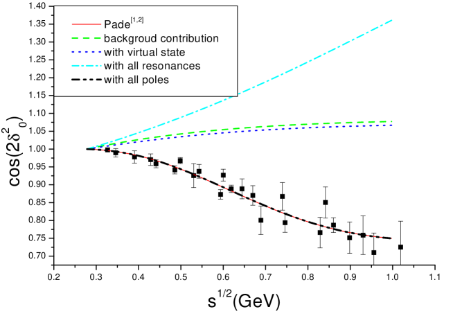
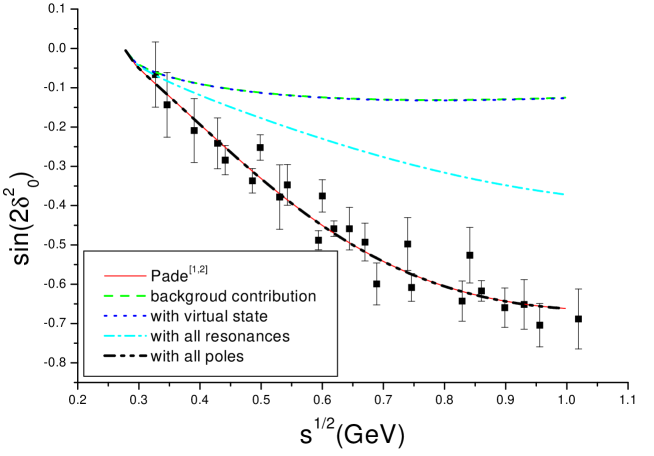
Figure 3: Various contributions to $\cos(2\delta^{2}_{0})$ and $\sin(2\delta^{2}_{0})$ in the IJ=20 channel using the values from Eq. (S0.Ex24). The virtual state contribution as represented by the difference between the dashed line and the dotted line is very small.

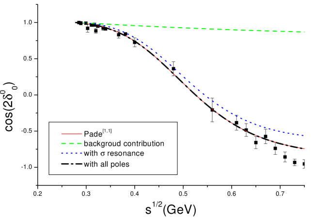
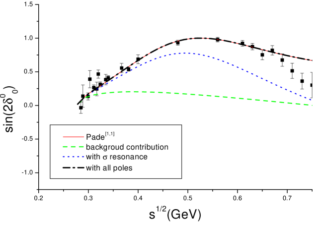
Figure 4: Various contributions to $\cos(2\delta^{0}_{0})$ and $\sin(2\delta^{0}_{0})$ in the IJ=00 channel using the values from Eq. (21), using the [1,1] Padé amplitude.

From above results we find that the $\chi^{2}$ fit is very insensitive to $\bar{l}_{3}$, $r_{1}$ and $r_{2}$. The other $r_{i}$ parameters are barely comparable in order of magnitude to those given in Eq. (S0.Ex23) [20]. The results for the fit are shown in table 2 and Figs. 1–3. In order to compare the [1,2] Padé results with [1,1] Padé results we also made the global fit in the latter case. The results are given in table 3. In Fig. 4 we plot the [1,1] Padé fit results in the most interesting IJ=00 channel. In Figs. 1 – 4, the solid lines represent the phase shift value directly obtained from the Padé amplitudes in the physical region, $i.e.$, $\delta_{\pi}(s)={\rm Atan}({{\rm Im}_{R}T(s)}/{{\rm Re}_{R}T(s)})$. The dash-dot-dot-dash lines in Figs. 1–3 and the dash-dot-dash line in Fig. 4 represent the summation of all contributions on the $r.h.s.$ of Eqs. (12) and (13) (also including SPSRs’ contributions). The two kinds of lines must coincide with each other as a consistency check of our numerical calculation.

IJ	Pole	Re[$s_{p}$]	Im[$s_{p}$]	Res$\tilde{F}$
00	$\sigma$	586MeV(M)	775MeV($\Gamma$)	–42.28+2.22i
	R	318MeV(M)	935MeV($\Gamma$)	18.28+15.41i
	SPSR	135.68	56.46	22.82+39.79i
11	$\rho$	768MeV(M)	150MeV($\Gamma$)	–1.55+6.13i
	R	678MeV(M)	1.02GeV($\Gamma$)	5.65–2.24i
	SPSR	0.83	39.17	–4.13+1.28i
20	VS	0.0483292	0	0.0451211
	R	647MeV(M)	2.34GeV($\Gamma$)	–31.05+41.92i
	R	299MeV(M)	7.27GeV($\Gamma$)	96.25–29.84i
	SPSR	–11.94	27.44	9.62–13.06i

Table 2: Resonances(R), spurious physical sheet resonances (SPSR) and virtual states (VS) as predicted by the [1,2] Padé approximation on the complex $s$ plane using the values from Eq. (S0.Ex24). The pole position $s_{p}=(M+i\Gamma/2)^{2}$. All numbers in the table are in unit of $m_{\pi}^{2}$ unless stated otherwise The fit values of the scattering length parameters are, $a^{0}_{0}=0.217,a^{2}_{0}=-0.0531$.

The coupling constants obtained from the fit using the [1,1] Padé amplitudes are the following,

$$\bar{l}_{1}=-0.33^{+0.067}_{-0.068}\ ,\ \bar{l}_{2}=5.83^{+0.067}_{-0.067}\ ,\ \bar{l}_{3}=24.09^{+11.24}_{-10.52}\ ,\ \bar{l}_{4}=3.51^{+0.27}_{-0.27}\ .$$ (21)

IJ	Pole	Re[$s_{p}$]	Im[$s_{p}$]	Res[$\tilde{F}$]
00	$\sigma$	456MeV(M)	463MeV($\Gamma$)	–4.77–6.47i
	SPSR	–74.50	53.35	–106.31–103.32i
11	$\rho$	751MeV(M)	144MeV($\Gamma$)	–2.55+4.99i
20	VS	0.0335461	0	0.0318398
	SPSR	103.30	351.11	–489.54+77.33i

Table 3: Resonances(R), spurious physical sheet resonances (SPSR) and virtual states (VS) as predicted by the [1,1] Padé approximation on the complex $s$ plane using the values from Eq. (18) and Eq.(S0.Ex23). The pole position $s_{pole}=(M+i\Gamma/2)^{2}$. All numbers in the table are in unit of $m_{\pi}^{2}$ unless stated otherwise. The fit values of the scattering length parameters are, $a^{0}_{0}=0.186,a^{2}_{0}=-0.0467$.

Comparing the results of [1,1] Padé approximants and the [1,2] Padé approximants we conclude that the [1,2] Padé approximation does not in general improve the bad situation the [1,1] Padé approximants encounter, though the former can give a better fit to the phase shift data. In the IJ=11 channel the [1,1] Padé amplitude only predict the $\rho$ resonance, in the [1,2] amplitude there are additional poles at distant positions but their contributions are rather small, so both the two amplitudes can be considered as phenomenologically successful. In the IJ=20 channel both amplitudes run into disaster since both of them predict huge contributions from SPSRs. Comparing Fig. 2 with Fig. 2 of Ref. [12] one finds that the [1,2] Padé amplitude is even worse in the sense that it predicts large SPSR contribution also to $\sin(2\delta)$. In fact the perturbation result in this channel is much better [13]. In the most interesting IJ=00 channel, the situation is more complicated. From Fig. 4 we find that the SPSR’s contribution to $\sin(2\delta$) is sizable yet in Fig. 1 the SPSR’s contribution is very small. However, in the latter case there appears another large contribution from a resonance ($R$) located at $s_{R}=(0.318\pm 0.468i)^{2}$GeV² in the IJ=00 channel, which is neither very far away from nor very close to the low energy physics region. When looking at table 2 one may even confuse the two resonances in the IJ=00 channel: the $\sigma$ and $R$. The two resonances are distinguishable in the following way: in table 1 one resonance pole is much closer to the physical region comparing with another one, the former is of course denoted as $\sigma$.  Then we can tune the parameters $\bar{l}_{i}$ and $r_{i}$ continuously, from the values given in Eqs. (18) and (S0.Ex23) to the central values of the parameters given in Eq. (S0.Ex24), and keep track of the pole positions. In this way we can distinguish the two resonance poles in table 2. Obviously the pole position of $R$ is very sensitive to the parameters of the chiral Lagrangian and the pole position of the $\sigma$ meson is rather stable. The former comes actually from very distant places, therefore its existence and contribution is still doubtful even though it is located not very far from the physical region as predicted by the parameter set determined from the global fit. In this sense one hesitates to conclude that the [1,2] Padé approximant in the IJ=00 channel is better than the [1,1] approximation even though the SPSRs’ contribution is reduced.

In above discussions we point out and study in details the problem of the Padé approximation method induced by the existence of SPSRs, which has not drawn much attention in the literature. It is worth mentioning that the author of Ref. [23] noticed such a problem and proposed a scheme to remedy the situation when studying the $\pi$ scalar form-factor, $F$, to two loops using IAM. When obtaining Eq. (7) from Eq. (6) in that paper, the author essentially did the following: expanding the SPSR term up to $O(s^{2})$ and neglecting the higher order terms, and reabsorb the coefficients of the second order polynomial into the low energy constants, and the latter are determined by either CHPT or by fit. In this way the SPSR (which, according to the author, locates on the negative real axis) is eliminated in the newly obtained $F$. This effort is respectable as it is in the right direction, but is still problematic. Actually it is not difficult to prove that the procedure proposed by the author does not make the effects of the spurious pole totally vanish but actually moves the pole from the 1st sheet to the 2nd sheet (see the appendix for the proof). A pole on the negative real axis on the 2nd sheet is still dubious, even though its numerical influence is not estimated.

To conclude, in general the prediction from the [1,2] Padé approximation is not in any sense more trustworthy than the [1,1] Padé approximation. A lesson one may draw from the discussion made in this paper is that physics at distant places (no matter spurious or not) as predicted by the Padé approximation do not necessarily decouple at low energies. We suggest, to make safe use of the Padé approximation one has to make a case by case analysis to the amplitudes using the method proposed in this paper. The smallness of the contribution from high energies may be considered as a necessary condition for the predictions of the Padé amplitude at moderately low energies to be numerically trustworthy.

This work is supported in part by China National Natural Science Foundation under grant number 10047003 and 10055003.

Appendix A Appendix

The proof follows: denote the formfactor defined in Eq. (6) in Ref. [23] by $F_{1}$ and that defined in Eq. (7) by $F$. The major difference between $F$ and $F_{1}$ is that the latter contains the SPSR. Especially we have Im$F$=Im$F_{1}$ and

$$F=P_{2}(s)+{s^{3}\over\pi}\int_{4m_{\pi}^{2}}^{\infty}ds^{\prime}\frac{{\rm Im}F(s^{\prime})}{s^{\prime 3}(s^{\prime}-s-i\epsilon)}\equiv{\rm Re}F(s)+i{\rm Im}F(s)\ .$$ (22)

This $F$, even though does not satisfy exact unitarity, maintains the two–sheet structure and can be analytically continued to the second sheet by changing the sign of the kinematic factor $\rho=\sqrt{1-4m_{\pi}^{2}/s}$, notice that both ${\rm Re}F(s)$ and $i{\rm Im}F(s)$ can be analytically continued to the complex $s$ plane. To be specific $F^{II}$ is,

$$F^{II}=P_{2}(s)+{s^{3}\over\pi}P\int_{4m_{\pi}^{2}}^{\infty}ds^{\prime}\frac{{\rm Im}F(s^{\prime})}{s^{\prime 3}(s^{\prime}-s)}-i{\rm Im}F(s)={\rm Re}F(s)-i{\rm Im}F(s)\ ,$$ (23)

$i.e.$, the $F^{II}$ is obtainable by just simply changing the sign of ${\rm Im}F(s)$ and $P$ stands for the principle value. By construction $F$ does not contain any poles on the entire cut plane and according to Ref. [23] $F^{II}$ does. That is possible only when both ${\rm Re}F(s)$ and $i{\rm Im}F(s)$ contain poles on the cut plane but cancel each other in ${\rm Re}F(s)+i{\rm Im}F(s)$, but not in ${\rm Re}F(s)-i{\rm Im}F(s)$. Therefore the pole locations of $F^{II}$ are the same as $i{\rm Im}F(s)$ and are also the same as $i{\rm Im}F_{1}(s)$. However it is clear from Eq. (6) of Ref. [23] that $i{\rm Im}F_{1}(s)$ contains the poles of $F_{1}$ on the 1st sheet (corresponding to zeros of $\Gamma^{(2)}$, for the definition of the latter see Ref. [23]), as well as poles on the 2nd sheet (corresponding to zeros of $\Gamma^{(2)*})$. Therefore all poles of $F_{1}$ are transmitted into $F^{II}$ including both the $\sigma$ pole and the spurious pole.

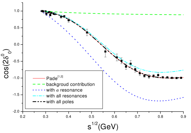
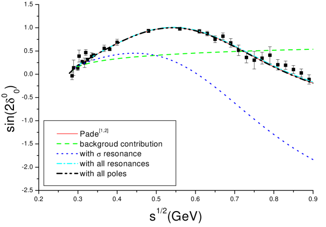
Figure 1: Various contributions to $\cos(2\delta^{0}_{0})$ and $\sin(2\delta^{0}_{0})$ in the IJ=00 channel using the values from Eq.(S0.Ex24). Notice that in the IJ=00 channel we only fit the data up to 730MeV. The [1,2] Padé amplitude gives a much better description to the data above 730MeV than the [1,1] Padé amplitude, see Fig. 4 for comparison. The solid line and the dash-dot-dot-dash line are explained in the text. The dashed line is from the background contribution only, whereas the dotted line represents the contributions from the $\sigma$ and the background, and the dash-dot-dash line is to add the resonance (R) contribution to the dotted line. The fact that the dash-dot-dash line is very close to the solid line indicates that the SPSR’s contribution is very small.

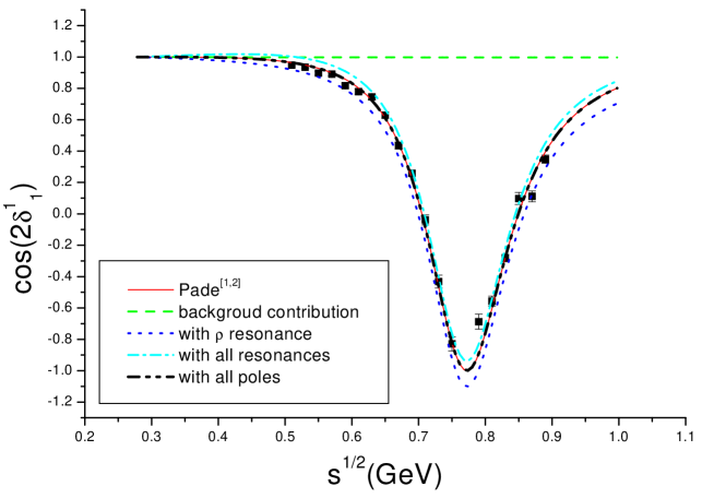
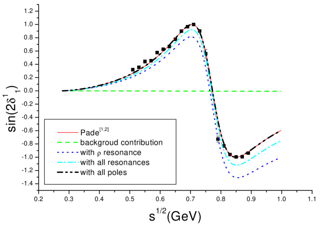
Figure 2: Various contributions to $\cos(2\delta^{1}_{1})$ and $\sin(2\delta^{1}_{1})$ in the IJ=11 channel using the values from Eq.(S0.Ex24). The meaning of different lines is similar to those in Fig. 1.

References

- [1] S. Weinberg, Phys. Rev. Lett. 17 (1966)616.
- [2] L. F. Li and H. Pagels, Phys. Rev. Lett. 26 (1971)1204.
- [3] J. Gasser and H. Leutwyler, Ann. Phys. (N.Y.) 158 (1984) 142.
- [4] J. Gasser and H. Leutwyler, Nucl. Phys. B 250 (1985) 465.
- [5] For a review, see for example, A. Pich, Introduction to Chiral Perturbation Theory, Lectures given at the V Mexican School of Particles and Fields, Guanajuato, México, December 1992, hep-ph/9308351.
- [6] H. W. Fearing and S. Scherer, Phys. Rev. D53(1996)315.
- [7] M. Knecht , Nucl. Phys. B457(1995)513.
- [8] J. Bijnens , Phys. Lett. B374(1996)210.
- [9] J. Bijnens , Nucl. Phys. B508(1997)263; Erratum-ibid. B517(1998)639.
-
[10]
A. Dobado, M. J. Herrero and T. N. Truong, Phys. Lett. B235, 134
(1990).
T. Hannah, Phys. Rev. D52, 4971 (1995).
A. Dobado and J. R. Peláez, Phys. Rev. D47, 4883 (1993); Phys. Rev. D56, 3057 (1997).
J. A. Oller, E. Oset and J. R. Peláez, Phys. Rev. Lett. 80, 3452 (1998); Phys. Rev. D59, 074001 (1999); (E)-ibid D60, 099906 (1999).
A. Gómez-Nicola and J. R. Peláez, Phys. Rev. D65, 054009 (2002). - [11] For a review article, see for example, J. A. Oller, E. Oset and A. Ramos, Prog. Part. Nucl. Phys. 45(2000)157.
- [12] Q. Ang , Commun. Theor. Phys. 36(2001)563 (hep-ph/0109012).
- [13] Z. G. Xiao and H. Q. Zheng, Nucl. Phys. A695(2001) 273; hep-ph/0103042.
- [14] J. Y. He, Z. G. Xiao and H. Q. Zheng, Phys. Lett. B536(2002) 59.
- [15] S. D. Protopopescu et al., Phys. Rev. D7 (1973) 1279.
- [16] G. Grayer et al., Nucl. Phys. B75 (1974) 189; W. Ochs, Ph.D. thesis, Munich Univ., 1974.
- [17] W. Maenner, in – 1974 (Boston), Proceedings of the fourth International Conference on Meson Spectroscopy, edited by D. A. Garelick, AIP Conf. Proc. No. 21 (AIP, New York, 1974).
- [18] L. Rosselet et al., Phys. Rev. D15(1977) 574.
- [19] P. Truöl (E865 Collaboration), hep-ex/0012012.
- [20] Discussions on the global fit using Padé amplitudes may also be found in: J. Nieves, M. Pavon-Valderrama and E. Ruiz-Arriola, Phys. Rev. D65(2002) 036002; F. Guerrero and J. A. Oller, Nucl. Phys. B537 (1999) 459.
- [21] T. Hatsuda and T. Kunihiro, To appear in the proceedings of International Workshop on Chiral Fluc, Orsay, France, 26-28 Sep 2001, nucl-th/0112027; M. J. Vicente Vacas and E. Oset, nucl-th/0204055.
- [22] E. van Beveren, F. Kleefeld, G. Rupp and M. D. Scadron, hep-ph/0204139.
- [23] T. Hannah, Phys. Rev. D60 (1999) 017502.