Signals for Lorentz Violation in Electrodynamics

Abstract

An investigation is performed of the Lorentz-violating electrodynamics extracted from the renormalizable sector of the general Lorentz- and CPT-violating standard-model extension. Among the unconventional properties of radiation arising from Lorentz violation is birefringence of the vacuum. Limits on the dispersion of light produced by galactic and extragalactic objects provide bounds of $3\times 10^{-16}$ on certain coefficients for Lorentz violation in the photon sector. The comparative spectral polarimetry of light from cosmologically distant sources yields stringent constraints of $2\times 10^{-32}$. All remaining coefficients in the photon sector are measurable in high-sensitivity tests involving cavity-stabilized oscillators. Experimental configurations in Earth- and space-based laboratories are considered that involve optical or microwave cavities and that could be implemented using existing technology.

I INTRODUCTION

Lorentz symmetry underlies the theory of relativity and all accepted theoretical descriptions of nature at the fundamental level. A crucial role in establishing both the rotation and boost components of Lorentz symmetry has been played by experimental studies of the properties of light. In the classic tests, rotation invariance is investigated in Michelson-Morley experiments searching for anisotropy in the speed of light, while boost invariance is studied via Kennedy-Thorndike experiments seeking a variation of the speed of light with the laboratory velocity [1, 2, 3].

In this work, a theoretical study is performed of various experiments testing Lorentz symmetry with light and other electromagnetic radiation. The analysis is within the context of the Lorentz- and CPT-violating standard-model extension [4], developed to allow for small general violations in Lorentz and CPT invariance [5]. The lagrangian of this theory includes all observer Lorentz scalars formed by combining standard-model fields with coupling coefficients having Lorentz indices. At the level of quantum field theory, the violations can be regarded as remnants of Planck-scale physics appearing at attainable energy scales. The coefficients for Lorentz violation may be related to expectation values of Lorentz tensors or vectors in an underlying theory [6]. To date, experimental tests of the standard-model extension have been performed with hadrons [7, 8, 9, 10], protons and neutrons [11], electrons [12, 13], photons [14, 15], and muons [16].

In the present context of studies of electrodynamics, the standard-model extension is of interest because it provides a general field-theoretic framework for investigating the Lorentz properties of light. The theory contains as a subset a general Lorentz-violating quantum electrodynamics (QED), which includes a general Lorentz-violating extension of the Maxwell equations. We study experiments that can measure the coefficients for Lorentz violation in this generalized electrodynamics. Our attention is restricted here to exceptionally sensitive experiments that could be in a position to detect the minuscule effects motivating the standard-model extension.

A basic feature of Lorentz-violating electrodynamics is the birefringence of light propagating in vacuo. This results in several potentially observable effects, including pulse dispersion and polarization changes. One goal of this work is to consider the implications of these effects for the propagation of radiation on astrophysical scales. We use available observations to constrain certain coefficients for Lorentz violation.

Another goal of this work is to analyze modern versions of some classic tests of special relativity based on resonant-cavity oscillators [17, 18, 19], which have extreme sensitivity to the properties of electromagnetic fields. These experiments depend on the Earth’s sidereal and orbital motion. However, the advent of the International Space Station (ISS) makes it feasible to perform laboratory experiments in space, where the orbital motion can yield different sensitivity to Lorentz-violating effects [20]. We consider here both space- and Earth-based laboratory experiments with resonant cavities.

The structural outline of this paper is as follows. Section II presents some basic results and definitions for the general Lorentz-violating electrodynamics and outlines the connection to some test models. We then consider birefringence experiments, beginning in Sec. III A with some general issues. Constraints stemming from the resulting effects on pulse dispersion from astrophysical sources are addressed in Sec. III B, while those from polarization changes over cosmological scales are treated in Sec. III C. A general analysis for laboratory-based experiments on the Earth and in space is presented in Sec. IV A. Sections IV B and IV C apply this analysis to experiments with optical and microwave resonant cavities. We summarize in Sec. V. Throughout this work, we adopt the conventions of Ref. [4].

II LORENTZ-VIOLATING ELECTRODYNAMICS

This section provides some background and contextual information about the general Lorentz-violating electrodynamics. The basic formalism is presented, and some definitions used in later sections are introduced. We also discuss the connection between this theory and some test models for Lorentz violation.

A Basic Theory

The standard model of particle physics is believed to be the low-energy limit of a fundamental theory that includes all the forces in nature. The natural scale of this fundamental theory is likely to be determined by the Planck mass. The possibility that Lorentz- and CPT-violating signals from this theory may be observable at energies attainable today led to the development of the standard-model extension [4], which is a general theory based on the standard model but allowing for violations of Lorentz and CPT symmetry [5]. The additional terms must be small because the usual standard model agrees well with experiment. They may originate from spontaneous symmetry breaking in the fundamental theory [6].

The standard-model extension can be defined as the usual standard-model lagrangian plus all possible additional Lorentz- and CPT-violating terms involving standard-model fields that maintain invariance under Lorentz transformations of the observer’s inertial frame. This invariance ensures that the physics is independent of the choice of coordinates. The Lorentz violation is associated with rotations and boosts of particles or localized field configurations in a fixed observer inertial frame.

Many of the detailed investigations of the standard-model extension have been performed under the simplifying assumption that the additional Lorentz- and CPT-violating terms preserve the SU(3)$\times$SU(2)$\times$U(1) local gauge symmetry of the usual standard model. Another widely adopted simplifying assumption is that the coefficients for Lorentz violation are independent of position. This implies the violation is restricted to the Lorentz symmetry instead of the full Poincaré symmetry and has several useful consequences for experiment, including the conservation of energy and momentum. It is also often convenient to restrict attention to the renormalizable sector of the theory, since this is expected to dominate the physics at low energies. However, nonrenormalizable terms are known to play an important role at higher energies [21].

Extracting terms involving the photon fields from the standard-model extension yields a Lorentz- and CPT-violating extension of QED [4]. The fermion sector of this theory has been widely studied. Here, we focus attention on the pure-photon sector and limit attention to the renormalizable terms, which involve operators of mass dimension four or less. The relevant lagrangian is [4]

$${\cal L} = -{\textstyle{{1}\over{4}}}F_{\mu\nu}F^{\mu\nu}+{\textstyle{{1}\over{2}}}(k_{AF})^{\kappa}\epsilon_{\kappa\lambda\mu\nu}A^{\lambda}F^{\mu\nu}$$ (2)

$$-{\textstyle{{1}\over{4}}}(k_{F})_{\kappa\lambda\mu\nu}F^{\kappa\lambda}F^{\mu\nu},$$

where $F_{\mu\nu}\equiv\partial_{\mu}A_{\nu}-\partial_{\nu}A_{\mu}$. This theory maintains the usual U(1) gauge invariance under the transformations $qA_{\mu}\to qA_{\mu}+\partial_{\mu}\Lambda$. The lagrangian contains the standard Maxwell term and two additional Lorentz-violating terms. The first of these extra terms is CPT odd, and its coefficient $(k_{AF})^{\kappa}$ has dimensions of mass. The other is CPT even. Its coefficient $(k_{F})_{\kappa\lambda\mu\nu}$ is dimensionless and has the symmetries of the Riemann tensor and a vanishing double trace, which implies a total of 19 independent components.

The CPT-odd term has received much attention in the literature [22]. This term provides negative contributions to the canonical energy and therefore is a potential source of instability. One solution is to set the coefficient to zero, $(k_{AF})^{\kappa}=0$. This is theoretically consistent with radiative corrections in the standard-model extension and is well supported experimentally: stringent constraints on $k_{AF}$ have been set by studying the polarization of radiation from distant radio galaxies [14].

In contrast, much less is known about the CPT-even coefficient $k_{F}$. Theoretical studies show that it provides positive contributions to the canonical energy and that it is radiatively induced from the fermion sector in the standard-model extension [4, 23]. Constraints on some components have recently been obtained from optical spectropolarimetry of cosmologically distant sources [15]. In the present work, we focus on the experimental implications of this CPT-even term. The coefficient $(k_{AF})^{\kappa}$ is set to zero for the analysis.

The equations of motion from lagrangian (2) are

$$\partial_{\alpha}{F_{\mu}}^{\alpha}+(k_{F})_{\mu\alpha\beta\gamma}\partial^{\alpha}F^{\beta\gamma}=0.$$ (3)

These are modified source-free inhomogeneous Maxwell equations. The homogeneous Maxwell equations,

$$\partial_{\mu}\widetilde{F}^{{\mu\nu}}\equiv{\textstyle{1\over 2}}\epsilon^{\mu\nu\kappa\lambda}\partial_{\mu}F_{\kappa\lambda}=0,$$ (4)

remain unchanged.

Although it lies beyond our present scope, the techniques presented here and the results obtained can be generalized to the nonrenormalizable sector. The nonrenormalizable terms can be classified according to their mass dimension. The dimensions of the corresponding coefficients are inverse powers of mass, and it is plausible that these coefficients are suppressed by corresponding powers of the Planck scale. Terms of this type appear in various special Lorentz-violating theories, including noncommutative field theories incorporating QED [24]. Indeed, any coordinate-independent theory with a photon sector containing nonrenormalizable Lorentz-violating terms must be a subset of the standard-model extension. It would be interesting to provide a detailed study of the nonrenormalizable terms in the Lorentz-violating electrodynamics and their experimental signals.

B Analogy and Definitions

A useful analogy exists between the Lorentz-violating electrodynamics in vacuo and the conventional situation in homogeneous anisotropic media [4]. The idea is to define fields $\vec{D}$ and $\vec{H}$ by the six-dimensional matrix equation

$$\left(\begin{array}[]{c}\vec{D}\\ \vec{H}\end{array}\right)=\left(\begin{array}[]{cc}1+\kappa_{DE}&\kappa_{DB}\\ \kappa_{HE}&1+\kappa_{HB}\end{array}\right)\left(\begin{array}[]{c}\vec{E}\\ \vec{B}\end{array}\right),$$ (5)

where $\vec{E}$ and $\vec{B}$ are the electric and magnetic fields obtained from solving the modified Maxwell equations (3). The $3\times 3$ matrices $\kappa_{DE}$, $\kappa_{HB}$, $\kappa_{DB}$, and $\kappa_{HE}$ are defined by

$$(\kappa_{DE})^{jk} = -2(k_{F})^{0j0k},$$ (6)

$$(\kappa_{HB})^{jk} = {\textstyle{1\over 2}}\epsilon^{jpq}\epsilon^{krs}(k_{F})^{pqrs},$$ (7)

$$(\kappa_{DB})^{jk} = -(\kappa_{HE})^{kj}=(k_{F})^{0jpq}\epsilon^{kpq}.$$ (8)

The double-trace condition on $(k_{F})_{\kappa\lambda\mu\nu}$ translates to the tracelessness of $(\kappa_{DE}+\kappa_{HB})$, while $(k_{F})_{\kappa[\lambda\mu\nu]}=0$ implies the tracelessness of $\kappa_{DB}=-(\kappa_{HE})^{T}$. This leaves $\kappa_{DE}$ and $\kappa_{HB}$ with eleven independent elements and the matrix $\kappa_{DB}=-(\kappa_{HE})^{T}$ with eight, which together represent the 19 independent components of $k_{F}$. Note also that $\kappa_{DE}$ and $\kappa_{HB}$ are parity even, while $\kappa_{DB}=-(\kappa_{HE})^{T}$ is parity odd.

With these definitions, the modified Maxwell equations (3), (4) take the familiar form

$$\vec{\nabla}\times\vec{H}-\partial_{0}{\vec{D}}=0, \quad\vec{\nabla}\cdot\vec{D}=0,$$ (9)

$$\vec{\nabla}\times\vec{E}+\partial_{0}{\vec{B}}=0, \quad\vec{\nabla}\cdot\vec{B}=0.$$ (10)

As a consequence, many results from conventional electrodynamics in anisotropic media also hold for this Lorentz-violating theory. For example, the energy-momentum tensor takes the standard form in terms of $\vec{E}$, $\vec{B}$, $\vec{D}$ and $\vec{H}$. This implies the usual Poynting theorem, which can be applied in conjunction with the symmetries of the matrices in Eq. (5) to show that the vacuum is lossless.

For the applications to be addressed in later sections, it is convenient to introduce the following decomposition of $(k_{F})_{\kappa\lambda\mu\nu}$ coefficients:

$$(\tilde{\kappa}_{e+})^{jk} = {\textstyle{1\over 2}}(\kappa_{DE}+\kappa_{HB})^{jk},$$ (11)

$$(\tilde{\kappa}_{e-})^{jk} = {\textstyle{1\over 2}}(\kappa_{DE}-\kappa_{HB})^{jk}-{\textstyle{{1}\over{3}}}\delta^{jk}(\kappa_{DE})^{ll},$$ (12)

$$(\tilde{\kappa}_{o+})^{jk} = {\textstyle{1\over 2}}(\kappa_{DB}+\kappa_{HE})^{jk},$$ (13)

$$(\tilde{\kappa}_{o-})^{jk} = {\textstyle{1\over 2}}(\kappa_{DB}-\kappa_{HE})^{jk},$$ (14)

$$\tilde{\kappa}_{\rm tr} = {\textstyle{{1}\over{3}}}(\kappa_{DE})^{ll}.$$ (15)

The first four of these equations define traceless $3\times 3$ matrices, while the last defines a single coefficient. All parity-even coefficients are contained in $\tilde{\kappa}_{e+}$, $\tilde{\kappa}_{e-}$ and $\tilde{\kappa}_{\rm tr}$, while all parity-odd coefficients are in $\tilde{\kappa}_{o+}$ and $\tilde{\kappa}_{o-}$. The matrix $\tilde{\kappa}_{o+}$ is antisymmetric while the other three are symmetric.

The form of this decomposition helps in determining the portion of the parameter space to which experiments are sensitive and how different experiments might overlap. For example, typical laboratory experiments with electromagnetic cavities search for rotation-violating parity-even observables. The sensitivity of such experiments is therefore expected to be dominantly to the ten rotation-violating parity-even coefficients $\tilde{\kappa}_{e+}$ and $\tilde{\kappa}_{e-}$. For those observables depending at leading order on the velocity, the eight coefficients $\tilde{\kappa}_{o+}$ and $\tilde{\kappa}_{o-}$ can be expected to play a role. Finally, at second order in the velocity one can expect the sole rotation-invariant quantity $\tilde{\kappa}_{\rm tr}$ to affect measurements. These considerations are confirmed by the results of the detailed analysis in the sections below.

As another example of the use of the decomposition (15), recall that birefringence is known to depend on ten linearly independent combinations of the components of $k_{F}$, which can be chosen as [15]

$$k^{a} = \bigl{(}(k_{F})^{0213},~{}(k_{F})^{0123},~{}$$ (20)

$$\>(k_{F})^{0202}-(k_{F})^{1313},~{}(k_{F})^{0303}-(k_{F})^{1212},~{}$$

$$\>(k_{F})^{0102}+(k_{F})^{1323},~{}(k_{F})^{0103}-(k_{F})^{1223},~{}$$

$$\>(k_{F})^{0203}+(k_{F})^{1213},~{}(k_{F})^{0112}+(k_{F})^{0323},~{}$$

$$\>(k_{F})^{0113}-(k_{F})^{0223},~{}(k_{F})^{0212}-(k_{F})^{0313}\bigr{)}.$$

Relating these to the $\tilde{\kappa}$ matrices, we find

$$(\tilde{\kappa}_{e+})^{jk} = -\left(\begin{array}[]{ccc}-(k^{3}+k^{4})&k^{5}&k^{6}\\ k^{5}&k^{3}&k^{7}\\ k^{6}&k^{7}&k^{4}\end{array}\right),$$ (24)

$$(\tilde{\kappa}_{o-})^{jk} = \left(\begin{array}[]{ccc}2k^{2}&-k^{9}&k^{8}\\ -k^{9}&-2k^{1}&k^{10}\\ k^{8}&k^{10}&2(k^{1}-k^{2})\end{array}\right).$$ (28)

In this way, we can see directly that birefringence is controlled by the matrices $\tilde{\kappa}_{e+}$ and $\tilde{\kappa}_{o-}$.

In terms of the $\kappa$ matrices defined in Eq. (8), and assuming as before that $(k_{AF})^{\alpha}=0$, the lagrangian (2) becomes

$${\cal L} = {\textstyle{1\over 2}}(\vec{E}^{2}-\vec{B}^{2})+{\textstyle{1\over 2}}\vec{E}\cdot(\kappa_{DE})\cdot\vec{E}-{\textstyle{1\over 2}}\vec{B}\cdot(\kappa_{HB})\cdot\vec{B}$$ (30)

$$+\vec{E}\cdot(\kappa_{DB})\cdot\vec{B}.$$

Similarly, using instead the $\tilde{\kappa}$ matrices defined in Eq. (15), we find

$${\cal L} = {\textstyle{1\over 2}}[(1+\tilde{\kappa}_{\rm tr})\vec{E}^{2}-(1-\tilde{\kappa}_{\rm tr})\vec{B}^{2}]$$ (33)

$$+{\textstyle{1\over 2}}\vec{E}\cdot(\tilde{\kappa}_{e+}+\tilde{\kappa}_{e-})\cdot\vec{E}-{\textstyle{1\over 2}}\vec{B}\cdot(\tilde{\kappa}_{e+}-\tilde{\kappa}_{e-})\cdot\vec{B}$$

$$+\vec{E}\cdot(\tilde{\kappa}_{o+}+\tilde{\kappa}_{o-})\cdot\vec{B}.$$

The form of Eq. (33) shows that a nonzero coefficient $\tilde{\kappa}_{\rm tr}$ shifts the effective permittivity $\epsilon$ and effective permeability $\mu$ by $(\epsilon-1)=-(\mu^{-1}-1)=\tilde{\kappa}_{\rm tr}$, corresponding to a shift in the speed of light. However, it is possible to remove an overall shift in the speed of light by making advantageous coordinate transformations accompanied by suitable field redefinitions, which combine to set $\epsilon=\mu^{-1}=1$ and transfer the Lorentz violation to a different sector of the theory. An explicit example of this procedure is provided in the next subsection for a toy model involving scalar QED.

In the general context of the standard-model extension, such transformations modify various other coefficients for Lorentz violation. In fact, similar transformations can move the nine independent coefficients $\tilde{\kappa}_{e-}$, $\tilde{\kappa}_{o+}$, and $\tilde{\kappa}_{\rm tr}$ into other sectors of the theory. Note that this effect is frame dependent because the coefficients mix under boosts. Note also that the possibility of absorbing $\tilde{\kappa}_{e-}$, $\tilde{\kappa}_{o+}$, $\tilde{\kappa}_{\rm tr}$ elsewhere offers insight as to why birefringence experiments, which directly compare light with light, are insensitive to these coefficients. However, cavity experiments involve comparisons of radiation with matter, so all 19 coefficients are observables in this case.

C Connection to Some Test Models

Several phenomenological test models for Lorentz properties of light have been proposed. The standard-model extension contains all observer-independent sources of Lorentz violation in terms of known particles, so it is expected to incorporate the existing test models as special cases. In this subsection, we comment on the relationships to some popular test models.

Since typical test models assume only one type of matter other than the photon, it suffices for our purposes to consider a toy version of the standard-model extension that includes only one scalar field and a limited type of Lorentz violation. We therefore work with a model of Lorentz-violating scalar QED, defined by the lagrangian

$${\cal L} = (\eta^{\mu\nu}+(k_{\phi})^{\mu\nu})(D_{\mu}\phi)^{\dagger}D_{\nu}\phi-m^{2}\phi^{\dagger}\phi$$ (35)

$$-{\textstyle{{1}\over{4}}}F_{\mu\nu}F^{\mu\nu}-{\textstyle{{1}\over{4}}}(k_{F})_{\kappa\lambda\mu\nu}F^{\kappa\lambda}F^{\mu\nu}.$$

In this expression, the covariant derivative takes the usual form, $D_{\mu}\phi=\partial_{\mu}\phi+iqA_{\mu}\phi$, and for simplicity we have limited the types of Lorentz violation to those described by a real symmetric coefficient $(k_{\phi})^{\mu\nu}$ and by a coefficient $(k_{F})_{\kappa\lambda\mu\nu}$ of the type in Eq. (2).

An interesting test model for Lorentz violation is provided by the kinematical framework of Robertson [25] and its extension to arbitrary synchronizations by Mansouri and Sexl [26]. These approaches suppose the existence of a “preferred” frame in which light propagates isotropically as measured by a standard set of rods and clocks. The Lorentz transformation between observers is then generalized to incorporate small changes from the conventional boosts in special relativity. Within a given synchronization, three parameters $g_{0}$, $g_{1}$, $g_{2}$ are needed to fix the generalized Lorentz transformation and hence to characterize the Lorentz violation.

The construction of the generalized Lorentz transformation can be illustrated in the context of the model (35). Consider the special case of the model for which only the coefficient $(k_{\phi})^{00}$ is nonzero in a certain frame $\Sigma$. Writing this coefficient as $(k_{\phi})^{00}=k^{2}-1$, where $k^{2}$ deviates slightly from 1, the lagrangian takes the form

$${\cal L} = (D_{\mu}\phi)^{\dagger}D^{\mu}\phi+(k^{2}-1)|D_{0}\phi|^{2}-m^{2}\phi^{\dagger}\phi$$ (37)

$$+{\textstyle{1\over 2}}(\vec{E}^{2}-\vec{B}^{2}).$$

In the $\Sigma$ frame, the propagation of light is rectilinear and isotropic, so it may be identified with the preferred frame of the test model. The Lorentz violation appears only in the $\phi$ sector of the lagrangian, which we can suppose describes the detailed physics of the rods or clocks in the test model.

The generalized Lorentz transformations ${T^{\mu}}_{\nu}$ considered in the kinematical test models are the linear transformations $x^{\prime\mu}={T^{\mu}}_{\nu}x^{\nu}$ from the preferred frame $\Sigma$ to a coordinate system $S$ attached to an observer moving at constant velocity in the preferred frame. By construction, the observer $S$ defines coordinates using the same rods and clocks and a prescribed synchronization. However, in the present context the Lorentz-violating properties of the rods and clocks are fixed by the Lorentz-violating scalar term in the lagrangian (37). The generalized Lorentz transformations ${T^{\mu}}_{\nu}$ from $\Sigma$ to $S$ are therefore also determined in the context of the model (35). They are the transformations leaving invariant the scalar sector and hence preserving the combination $\eta^{\mu\nu}+(k_{\phi})^{\mu\nu}$ up to a possible resynchronization. For example, for the special case of Eq. (37), the Robertson parameters are found to be $g_{0}=1/g_{1}=\sqrt{(1-\beta^{2})/(1-k^{2}\beta^{2})}$, $g_{2}=1$. The corresponding Mansouri-Sexl parameters are $a=1/b=\sqrt{(1-k^{2}\beta^{2})}$, $d=1$, with $\epsilon=-\beta(1-k^{2}\beta^{2})/(1-\beta^{2})$ in Einstein synchronization or $\epsilon=-k^{2}\beta$ in slow-clock synchronization. In contrast, the standard Lorentz transformations ${\Lambda^{\mu}}_{\nu}$ preserve $\eta^{\mu\nu}$.

In this simple example, the transformation ${T^{\mu}}_{\nu}$ leaves invariant the rods and clocks, while ${\Lambda^{\mu}}_{\nu}$ leaves invariant the speed of light. Both are equally valid. In the frames related by ${T^{\mu}}_{\nu}$, observers agree on rod lengths and clock rates but disagree on the velocity of light. Moreover, the velocity of light is no longer isotropic as measured by these rods and clocks. In contrast, observers related by Lorentz transformations agree that light propagates isotropically with speed 1 but may disagree on rod lengths and clock rates. The description is a matter of coordinate choice, and one can move freely from one to the other using ${T^{\mu}}_{\nu}$, ${\Lambda^{\mu}}_{\nu}$, and their inverses.

Note that a “preferred” frame in which light propagates isotropically typically fails to exist in the full standard-model extension, although in principle one can impose the existence of such a frame by suitably restricting the coefficients for Lorentz violation. From this perspective, the special status enjoyed by photons relative to other particles in the kinematical test models appears somewhat unnatural, and the structure of the standard-model extension offers more general possibilities for kinematical frameworks. Note also that the standard-model extension addresses modifications to all known particles, so the effects on physical rods and clocks can be directly analyzed. This is infeasible in kinematical frameworks, which consider the transformations between frames rather than the underlying physics.

Another interesting test model is the $c^{2}$ model [27], developed for application to studies of Lorentz invariance as a limiting case of the $TH\epsilon\mu$ formalism [28, 29]. The $c^{2}$ model is defined by a lagrangian describing the behavior of classical pointlike test particles in the presence of electromagnetic fields. The model assumes the existence of a “preferred” frame in which the limiting speed of the test particles is 1, while the speed of light is $c$.

To see the relation between the $c^{2}$ model and the model (35), consider another lagrangian written in a frame $S$ as

$${\cal L} = (D_{\mu}\phi)^{\dagger}D^{\mu}\phi-m^{2}\phi^{\dagger}\phi+{\textstyle{1\over 2}}(\vec{E}^{2}-k^{2}\vec{B}^{2}),$$ (38)

where $k^{2}$ deviates slightly from 1 as before. In this theory, the Lorentz violation appears in the photon sector. With the identification $k=c$, the lagrangian for this sector is identical to that of the $c^{2}$ model. Moreover, the $\phi$ sector is conventional, representing a quantum field theory of minimally coupled scalar particles. The model (38) can therefore be regarded as the field-theoretic equivalent of the $c^{2}$ model.

The two models (38) and (37) are related by the coordinate transformation $t\to t/k$, $\vec{x}\to\vec{x}$ followed by the field redefinition $A_{\mu}\to A_{\mu}/k$ and charge rescaling $q\to kq$. They therefore describe the same physics. Although it is possible to choose coordinates so that either the photon or the scalar propagates conventionally, the Lorentz violation cannot be eliminated simultaneously from both sectors.

We thus see that the $c^{2}$ model is contained in the theory (35) as a special case. In the terminology of Eq. (15), the parameter $c^{2}$ could be identified with the combination of coefficients $(1-\tilde{\kappa}_{\rm tr})/(1+\tilde{\kappa}_{\rm tr})$, as can be seen from Eq. (33). However, caution is required in interpreting bounds obtained with the $c^{2}$ model in terms of $\tilde{\kappa}_{\rm tr}$ because the identification is valid only in a frame $S$ with conventional particles, which typically fails to exist in the standard-model extension.

III ASTROPHYSICAL TESTS

In this section, we consider radiation propagating in free space. The Lorentz-violating electrodynamics predicts birefringence, which allows sensitive tests of Lorentz symmetry from observations of radiation propagated over astrophysical distances. We begin with some general theory, and then we obtain two sets of bounds on Lorentz violation from velocity and birefringence constraints.

A General Theory

The basic features of plane-wave solutions to the Lorentz-violating electrodynamics have been presented in Refs. [4, 15], so only relevant essentials are given here. With the standard ansatz $F_{\mu\nu}(x)=F_{\mu\nu}(p)e^{-ip_{\alpha}x^{\alpha}}$ for a plane wave with wave 4-vector $p^{\alpha}=(p^{0},\vec{p})$, the equation determining the dispersion relation and the electric field $\vec{E}$ is the modified Ampère law

$$M^{jk}E^{k}\equiv(-\delta^{jk}p^{2}-p^{j}p^{k}-2(k_{F})^{j\beta\gamma k}p_{\beta}p_{\gamma})E^{k}=0\ .$$ (39)

The dispersion relation is obtained as usual by requiring vanishing determinant of $M^{jk}$. It suffices for our present purposes to consider only leading-order effects in the coefficients $(k_{F})_{\kappa\lambda\mu\nu}$ for Lorentz violation. To leading order, one finds

$$p^{0}_{\pm}=(1+\rho\pm\sigma)|\vec{p}|\ ,$$ (40)

where

$$\rho = -{\textstyle{1\over 2}}{\tilde{k}_{\alpha}}^{\phantom{al}\alpha},\quad\sigma^{2}={\textstyle{1\over 2}}(\tilde{k}_{\alpha\beta})^{2}-\rho^{2},$$ (41)

with

$$\tilde{k}^{\alpha\beta} = (k_{F})^{\alpha\mu\beta\nu}{\hat{p}}_{\mu}{\hat{p}}_{\nu},\quad{\hat{p}}^{\mu}={p^{\mu}}/{|\vec{p}|}.$$ (42)

Note that ${\vec{p}}^{2}\rho$ and ${\vec{p}}^{2}\sigma$ are observer Lorentz scalars, which implies $\rho$ and $\sigma$ are scalars under observer rotations.

The dispersion relation (40) has two solutions, with corresponding electric fields $\vec{E}_{\pm}$. In conventional electrodynamics, the dispersion relation is $p^{0}=|\vec{p}|$ and all fields $\vec{E}$ perpendicular to $\vec{p}$ are solutions, so the propagation is independent of the polarization. However, in the present case the propagation is goverened by two specific modes $\vec{E}_{\pm}$, with the general solution to Eq. (39) being any linear combination of the two. This leads to birefringence: light generically has two components, each propagating independently.

There are several possible definitions for the velocity of the radiation, including the phase velocity $v_{p}^{j}\equiv p_{0}p^{j}/{\vec{p}}^{2}$, the group velocity $v_{g}^{j}\equiv({\vec{\nabla}_{\vec{p}})^{j}}p^{0}$, and the velocity of energy transport $v_{e}^{j}\equiv\theta^{j0}/\theta^{00}$, where $\theta^{\mu\nu}$ is the energy-momentum tensor. With the analogy discussed in Sec. II B, one can show by standard arguments that $\vec{v}_{g}=\vec{v}_{e}$ for a wave with fixed $\vec{p}$. Also, Eq. (40) can be used to find explicit leading-order expressions for the magnitudes of the phase and group velocities. We thereby obtain $v_{p}=v_{g}=v_{e}=1+\rho\pm\sigma$ to leading order in $(k_{F})_{\kappa\lambda\mu\nu}$. Note also that, to leading order, we can write $\hat{p}^{\alpha}=(p^{0},\vec{p})/|\vec{p}|\approx(1,\hat{v})$ in the expressions (41) for $\rho$ and $\sigma$. The quantity $\hat{v}$ can be regarded as the direction of propagation of the radiation, since the difference between it and the other velocities arises only at higher order and is irrelevant here.

The mode dependence of the velocity offers interesting possibilities for experimental tests of the theory. The velocity difference is

$$\Delta v\equiv v_{+}-v_{-}=2\sigma,$$ (43)

and is expected to be tiny. However, for sufficiently large path lengths this difference might become apparent in the form of observable effects on the pulse shape or the polarization of radiation. In the next two subsections, we exploit these features to obtain constraints on $(k_{F})_{\kappa\lambda\mu\nu}$.

An explicit form for the solutions $\vec{E}_{\pm}$ is needed for some of the analysis. Using the dispersion relation (40), the matrix in the Ampère law (39) can be written

$$M_{\pm}^{jk}=-[2(\rho\pm\sigma)\delta^{jk}+\hat{p}^{j}\hat{p}^{k}-2\tilde{k}^{jk}]\vec{p}^{\>2}.$$ (44)

The form of this matrix shows that the solutions $\vec{E}_{\pm}$ are wavelength independent but vary with the direction of propagation. Also, at leading order in $(k_{F})_{\kappa\lambda\mu\nu}$ the difference $M_{+}-M_{-}$ is proportional to the identity, so the leading-order solutions $\vec{E}_{+}$ and $\vec{E}_{-}$ are perpendicular. In fact, at leading order, $\vec{E}_{\pm}$ are perpendicular to $\vec{p}$ as well.

To express $\vec{E}_{\pm}$ explicitly, a choice of inertial frame must be made. It is convenient to adopt a standard reference frame to report the results of observations and hence ultimately to place constraints on the set of coefficients $k_{F}$.

A natural choice for the reference frame is a Sun-centered celestial equatorial frame with the $Z$-axis aligned along the celestial north pole at equinox 2000.0. The $Z$-axis is then at a declination of $90^{\circ}$, and the $X$- and $Y$-axes lie at declination $0^{\circ}$ and can be chosen to be at right ascension $0^{\circ}$ and $90^{\circ}$, respectively. The unit vector $\hat{X}$ thus points towards the vernal equinox on the celestial sphere. The time $T$ is chosen such that $T=0$ when the Earth crosses the $XY$ plane on a descending trajectory. In what follows, we adopt this standard frame to report results.

For the practical determination of $\vec{E}_{\pm}$ for a given wave, it is easiest first to work in a special ‘primed’ frame chosen for that wave. The result of the calculation can then be related to the standard Sun-centered frame by performing a suitable observer rotation. A convenient primed frame for a given wave is the frame in which the wave 4-vector takes the form $\hat{p}^{\prime\alpha}=(1;0,0,1)$ to leading order. The solution for $\vec{E}_{\pm}$ can be expressed explicitly in terms of the coefficients $k_{F}^{\prime}$ in this frame. Up to a normalization, it is found to be $\vec{E}_{\pm}\propto(\sin\xi,\pm 1-\cos\xi,0)$, where $\tan\xi=2\tilde{k}^{\prime\,12}/(\tilde{k}^{\prime\,11}-\tilde{k}^{\prime\,22})$. The two modes are thus linearly polarized.

From the solutions $\vec{E}_{\pm}$ and dispersion relation, it is evident that $\sigma$ and $\xi$ are the relevant parameters for birefringent effects for a particular source. In particular, $\sigma\sin\xi=\tilde{k}^{\prime\,12}$ and $\sigma\cos\xi={\textstyle{1\over 2}}(\tilde{k}^{\prime\,11}-\tilde{k}^{\prime\,22})$ represent the minimal linear combinations of $k_{F}^{\prime}$ that govern birefringence. The parameter $\rho$ is common to both modes, but does not contribute to birefringence and cannot be detected in the experiments discussed below.

The results in the primed frame can be related to the standard frame by a suitable observer rotation, described in Appendix A. The direction of travel of the light in the standard frame determines two vectors $\varsigma_{s}^{a}$ and $\varsigma_{c}^{a}$ in $k^{a}$ space (see Eq. (A25)), and it turns out that the birefringence of the light depends on the two specific linear combinations of the coefficients $k^{a}$ in Eq. (20) that are parallel to these vectors.

B Velocity constraints

For the two radiation modes $\vec{E}_{\pm}$ propagating over a distance $L$, the velocity difference (43) induces a difference $\Delta t\approx\Delta vL$ between the two travel times. Local measurements made on radiation emitted as a single burst from a distant source can therefore provide sensitivity to the coefficients $k^{a}$ for Lorentz violation [30].

To apply this idea, it is useful to consider distant sources that produce radiation in a relatively narrow burst characterized by a small width $w$, such as millisecond pulsars or sources of gamma-ray bursts. These sources typically produce essentially unpolarized radiation, so the intensity of each mode should be comparable. The burst can then be regarded as a superposition of two independently propagating pulses, one for each mode. For a sufficiently great distance $L$, a nonzero $\Delta v$ would cause the two pulses to separate enough to become distinguishable. This type of signal would manifest itself as two pulses with similar time structure but differing in arrival time. The pulses would each be linearly polarized, and they would have mutually perpendicular polarization angles.

If only a single pulse is observed, a limit on Lorentz violation can be deduced. The relationship between the observed pulse width $w_{o}$ and the source pulse width $w_{s}$ is approximately $w_{o}\approx w_{s}+\Delta t$. Observations of $w_{o}$ can therefore be used to obtain a conservative bound on $\Delta t=\Delta vL=2\sigma L$ and hence a bound on the coefficients $k^{a}$.

Source	$L$		$w_{o}$		Ref.
GRB 971214	2.2	Gpc	50	s	[31, 32]
GRB 990123	1.9	Gpc	100	s	[32, 33]
GRB 980329	2.3	Gpc	50	s	[32, 34]
GRB 990510	1.9	Gpc	100	s	[32, 35]
GRB 000301C	2.0	Gpc	10	s	[36, 37]
PSR J1959+2048	1.5	kpc	64	$\mu$s	[38]
PSR J1939+2134	3.6	kpc	190	$\mu$s	[38]
PSR J1824-2452	5.5	kpc	300	$\mu$s	[38]
PSR J2129+1210E	10.0	kpc	1.4	ms	[38]
PSR J1748-2446A	7.1	kpc	1.3	ms	[38]
PSR J1312+1810	19.0	kpc	4.4	ms	[38]
PSR J0613-0200	2.2	kpc	1.4	ms	[38]
PSR J1045-4509	3.2	kpc	2.2	ms	[38]
PSR J0534+2200	2.0	kpc	10	$\mu$s	[38, 39]
PSR J1939+2134	3.6	kpc	5	$\mu$s	[38, 40]

Table 1. Source data for velocity constraints.

Table 1 lists data for fifteen sources suitable for placing this type of constraint. The first five lines list gamma-ray bursts with known redshifts. The widths listed for these contain all significant time structure of the pulse. The distance $L$ is determined from the redshift by the look-back time in a conservative cosmology for a matter-dominated universe with Hubble constant $H_{0}=80$ km s^-1 Mpc^-1. The next eight sources in the table are millisecond pulsars. The listed pulse width is that at $10\%$ peak intensity. The final two sources are giant-pulse pulsars. These exhibit intense pulses with characteristic widths on the order of several $\mu$s.

For each source in Table 1, we take $\sigma\leq w_{o}/2L$ as a bound on $\sigma$. For a single source, this places constraints on a two-dimensional subspace of the full 10-dimensional parameter space of the coefficients $k^{a}$. The subspace is represented by the linear combinations $\sigma\sin\xi$ and $\sigma\cos\xi$ associated with that particular source. To bound all ten coefficients $k^{a}$, ten linearly independent constraints of this type are needed. This is feasible using five or more sources at different positions on the sky.

We proceed by assuming the constraint for each source in Table 1 is consistent with a measurement of $\sigma=0$, and we take the bound $\sigma\leq w_{o}/2L$ as a reasonable estimate of the error in a null measurement. The associated $\chi^{2}$ distribution is $\chi^{2}=\sum 4L^{2}\sigma^{2}/w_{o}^{2}$, where the sum is over the fifteen sources. This is a quadratic form in $k^{a}$. Considering $|k^{a}|$ and minimizing $\chi^{2}$ with respect to the other nine degrees of freedom, we obtain a bound of

$$|k^{a}|<3\times 10^{-16}$$ (45)

in the Sun-centered celestial equatorial frame, at the $90\%$ confidence level.

This bound is much less stringent than that obtained through polarization measurements, as discussed below. However, the method is relatively straightforward and avoids some of the complexities involved in the polarization analysis.

C Polarization constraints

In this subsection, we expand on the material found in Ref. [15]. An improvement on the previous result is made by considering the cosmological redshift of light.

A general electric field $\vec{E}$ can be decomposed into its birefringent components $\vec{E}_{\pm}$. Defining unit vectors $\hat{\varepsilon}\pm=\vec{E}_{\pm}/|\vec{E}_{\pm}|$, the decomposition is

$$\vec{E}(x)=(E_{+}\hat{\varepsilon}_{+}e^{-ip^{0}_{+}t}+E_{-}\hat{\varepsilon}_{-}e^{-ip^{0}_{-}t})e^{i\vec{p}\cdot\vec{x}}.$$ (46)

The differing phase velocities of the two modes results in a change in relative phase as the wave propagates, given by [15]

$$\Delta\phi=(p^{0}_{+}-p^{0}_{-})t\approx 2\pi\Delta v_{p}L/\lambda\approx 4\pi\sigma L/\lambda,$$ (47)

where $\Delta v_{p}$ is the difference in phase velocities, $\lambda$ is the wavelength, and $L$ is the distance traveled. The phase change modifies the polarization state of the radiation, with larger effect for more distant sources. Appendix B provides a brief review of pertinent concepts involving polarization in the present context.

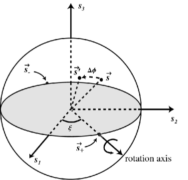
FIG. 1.: Rotation of the Stokes vector about $\vec{s}_{+}=-\vec{s}_{-}$.

In the primed frame described in Sec. III A, the Stokes vectors for $\hat{\epsilon}_{\pm}$ are $\vec{s}_{\pm}=\pm(\cos\xi,\sin\xi,0)$. These vectors correspond to opposite points on the equator of the Poincaré sphere, as expected for linearly polarized modes. As described in Appendix B, the axis of rotation induced by the phase change $\Delta\phi=4\pi\sigma L/\lambda$ is therefore in the $s^{1}$-$s^{2}$ plane. This affects both $\psi$ and $\chi$, as can be seen from Fig. 1.

A change in phase can arise from a change in either $L$ or $\lambda$. The induced change in the polarization depends not only on $k_{F}$ but also on the initial polarization. For cosmological sources, it may be impossible to determine independently the polarization at the source, in which case one cannot determine whether a change in polarization is strictly due to a change in $L$. It is therefore of more interest to focus on the wavelength dependence of the polarization change. Making the reasonable assumption that the emitted polarization is relatively constant over a given range of wavelengths, the relevant quantity becomes the phase shift as a function of wavelength,

$$\delta\phi=4\pi\sigma L\bigr{(}{{1}\over{\lambda}}-{{1}\over{\lambda_{0}}}\bigl{)},$$ (48)

relative to a reference wavelength $\lambda_{0}$. Standard spectropolarimetric techniques then allow a measurement of this effect. Note that knowledge of physical processes in certain classes of objects producing the polarized radiation might make it feasible to include a known initial polarization in the analysis, but this is unlikely to improve significantly the constraint obtained here.

The effect on the measured polarization as the wavelength is changed can be visualized using the Poincaré sphere. Suppose a source produces radiation with constant polarization over a range of wavelengths. This radiation can be represented by a single point on the Poincaré sphere. As the light propagates towards the Earth, the presence of Lorentz violation causes this point to rotate along an arc on the sphere. For any fixed wavelength, the rotation axis and rate depend on the coefficients $(k_{F})_{\kappa\lambda\mu\nu}$ and on the position of the source on the sky. However, Eq. (48) shows that shorter wavelengths rotate more than longer ones. Therefore, as measurements of the Stokes vector are made over a range of wavelengths, the results trace a circular arc on the surface of the Poincaré sphere.

Let $\psi_{0}$ and $\chi_{0}$ represent the observed polarization of a point on this arc with the reference wavelength $\lambda_{0}$. Using this point as a reference, we require the change in polarization relative to this point induced by Eq. (48). This polarization change is given by

$$s^{j}(\psi,\chi)=m^{jk}(\delta\phi)s^{k}(\psi_{0},\chi_{0}),$$ (49)

where $m^{jk}$ is the rotation matrix about $\vec{s}_{+}$ by $\delta\phi$. The matrix $m^{jk}$ is analogous to the Mueller matrix used in polarimetry to describe the effects of various filters and polarizers on light. Its explicit form is given as Eq. (8) of Ref. [15]. The angle $\chi$, which controls the amount of circular polarization, is absent from most published spectropolarimetric data. It is therefore most effective to focus attention on the change $\delta\psi=\psi-\psi_{0}$ in $\psi$ from the reference value $\psi_{0}$, which is given as Eq. (9) of Ref. [15]. A procedure for fitting this equation to existing spectropolarimetric data is also provided in this reference, and a 90% confidence-level bound of $|k^{a}|<3\times 10^{-32}$ is obtained from spectropolarimetric data for 16 cosmological sources.

In the present work, we use the same procedure to obtain a slight improvement on the existing bound by incorporating the redshift of the light as it propagates to the Earth. Cosmological redshift implies that over the path traveled the light has shorter wavelength than observed. Taking the same conservative cosmology as in the previous subsection and integrating the phase change over the propagation time yields

$$\Delta\phi={{4\pi\sigma}\over{\lambda}}{{2}\over{H_{0}}}\bigl{(}1-{{1}\over{\sqrt{1+z}}}\bigr{)},$$ (50)

where $\lambda$ is the observed wavelength and $z$ is the redshift. To account for the redshift, it therefore suffices to replace $L$ with $L_{\rm eff}=2(1-(1+z)^{-1/2})/H_{0}$ in the analysis.

Source	$L_{eff}$ (Gpc)	$10^{30}L_{eff}/\lambda$	$\log_{10}\sigma$
IC 5063 [41]	0.04	0.56 - 2.8	-30.8
3A 0557-383 [42]	0.12	2.2 - 8.5	-31.2
IRAS 18325-5925 [42]	0.07	1.0 - 4.9	-31.0
IRAS 19580-1818 [42]	0.14	1.8 - 9.3	-31.0
3C 324 [43]	2.44	82 - 180	-32.3
3C 256 [44]	3.04	110 - 220	-32.4
3C 356 [45]	2.30	78 - 170	-32.3
F J084044.5+…[46]	2.49	88 - 170	-32.4
F J155633.8+…[46]	2.75	99 - 160	-32.4
3CR 68.1 [47]	2.48	84 - 180	-32.4
QSO J2359-1241 [48]	2.01	110 - 120	-31.2
3C 234 [49]	0.61	55 - 81	-31.7
4C 40.36 [50]	3.35	120 - 260	-32.4
4C 48.48 [50]	3.40	120 - 260	-32.4
IAU 0211-122 [50]	3.40	120 - 260	-32.4
IAU 0828+193 [50]	3.53	130 - 270	-32.4

Table 2. Source data for polarization constraints.

Table 2 lists 16 sources with published values of $\psi$. The second column of the table displays the effective distance $L_{\rm eff}$ traveled by the light. The third column provides the range of wavelengths for which data are used. In fitting to $\delta\psi$, we choose to set $\psi_{0}$ equal to the mean value of the measured $\psi$. For each source, $\chi_{0}$ and $\lambda_{0}$ are fitted to the data. These angles can be thought of as the two degrees of freedom needed to describe the unknown polarization at the source. Ideally, at this point the data would be fitted to all the sources simultaneously. However, since $k^{a}$ has 10 elements and each source introduces two additional parameters, this would be involved. Instead, we examine each source individually and look for the desired wavelength dependence.

Adopting the same analysis strategy as described in Ref. [15] yields the bounds for each source listed in the last column of Table 2, which can be combined to yield a bound of

$$|k^{a}|<2\times 10^{-32}$$ (51)

in the Sun-centered celestial equatorial frame, at the $90\%$ confidence level.

IV LABORATORY TESTS

The Lorentz-violating electrodynamics predicts shifts in cavity-resonance frequencies, which offers the opportunity for sensitive tests of Lorentz symmetry in laboratories on the Earth and in space. This section presents a general framework for the analysis of such experiments. We begin with some general considerations and then separately consider in more detail the cases of optical cavities and microwave cavities.

A General Considerations

Many tests of special relativity search for variations in some observable that might arise from the rotation or boost of the apparatus due to the motion of the Earth. Lorentz-violating theories predict periodic variations at multiples of the Earth’s sidereal or orbital frequencies. For example, high-sensitivity measurements of coefficients in the fermion sector of the standard-model extension have been performed by comparing two clocks as the Earth rotates [11]. The clocks are typically the frequencies associated with specific Zeeman atomic transitions, and the standard-model extension predicts variations in these frequencies with the orientation of the apparatus and hence with the Earth’s rotation. Similar tests could be performed in space, with the frequency variations depending on the orbital and rotational properties of the spacecraft [20].

Resonant cavities can also serve as clocks, and they can be used in clock-comparison experiments to test properties of electromagnetic fields instead of atomic transitions. In particular, clock-comparison experiments of this type can be used to probe the photon sector of the standard-model extension. One relevant issue in the analysis of these experiments is establishing the transformation between the laboratory frame and a standard celestial frame. Another is the determination of the predicted frequency shifts. In this subsection, these issues are addressed in a general context.

1 Generic laboratory experiment

Consider a general laboratory-based experiment measuring some electrodynamic observable ${\cal O}$. Typically, the constitutive relations (5) change the observable from its conventional value ${\cal O}_{0}$. We consider a change $\delta{\cal O}$, taken to be linear in the matrices $\kappa_{DE}$, $\kappa_{HB}$, and $\kappa_{DB}=-\kappa_{HE}^{T}$. In a frame fixed to the laboratory, $\delta{\cal O}$ can be written as

$$\delta{\cal O} = ({\cal M}_{DE})^{jk}_{\rm lab}(\kappa_{DE})^{jk}_{\rm lab}+({\cal M}_{HB})^{jk}_{\rm lab}(\kappa_{HB})^{jk}_{\rm lab}$$ (53)

$$+({\cal M}_{DB})^{jk}_{\rm lab}(\kappa_{DB})^{jk}_{\rm lab},$$

where $({\cal M}_{DE})_{\rm lab}$, $({\cal M}_{HB})_{\rm lab}$, and $({\cal M}_{DB})_{\rm lab}$ are experiment-specific constant matrices determined by the apparatus. The symmetries of the $\kappa$ matrices can be imposed on their ${\cal M}$ counterparts when convenient.

Due to the orbital and rotational motion of the Earth or the space platform, the laboratory cannot be considered an inertial frame. As a result, the laboratory-frame coefficients $(\kappa_{DE})^{jk}_{\rm lab}$, $(\kappa_{HB})^{jk}_{\rm lab}$, and $(\kappa_{DB})^{jk}_{\rm lab}$ vary in time. We can exploit the induced variation in ${\cal O}$ by searching for periodic fluctuations in ${\cal O}$ at the relevant frequencies. A measurement of this type of variation would be a signal for Lorentz violation.

To determine the dependence of the periodic variation on the coefficients $(k_{F})_{\kappa\lambda\mu\nu}$, we seek an expression similar to Eq. (53) in an inertial frame. A suitable choice for a standard inertial frame is the Sun-centered celestial equatorial frame defined in Sec. III A. The coefficients for Lorentz violation in this frame, $(\kappa_{DE})^{JK}$, $(\kappa_{HB})^{JK}$, and $(\kappa_{DB})^{JK}$, are constant.

The observer Lorentz transformation between the two frames can be used to relate the corresponding two sets of $\kappa$ matrices. Since the velocity of the Earth with respect to the Sun is $\beta_{\oplus}\approx 10^{-4}$, it suffices for our purposes to construct the transformation to leading order. At this order, the Lorentz matrix $\Lambda^{\mu}_{\phantom{\mu}\nu}$ implementing the transformation from the Sun-centered frame to the laboratory frame is

$$\Lambda^{0}_{\phantom{0}T}=1,\ \ \Lambda^{0}_{\phantom{0}J}=-\beta^{J},\ \ \Lambda^{j}_{\phantom{j}T}=-(R\cdot\vec{\beta})^{j},\ \ \Lambda^{j}_{\phantom{j}J}=R^{jJ},$$ (54)

where $\vec{\beta}$ is the velocity of the laboratory with respect to the Sun-centered frame and $R^{jJ}$ is the spatial rotation from the Sun-centered frame to the laboratory frame. Some calculation shows that the induced transformation between the $\kappa$ matrices is

$$(\kappa_{DE})_{\rm lab}^{jk} = T_{0}^{jkJK}(\kappa_{DE})^{JK}-T_{1}^{(jk)JK}(\kappa_{DB})^{JK},$$ (55)

$$(\kappa_{HB})_{\rm lab}^{jk} = T_{0}^{jkJK}(\kappa_{HB})^{JK}-T_{1}^{(jk)KJ}(\kappa_{DB})^{JK},$$ (56)

$$(\kappa_{DB})_{\rm lab}^{jk} = T_{0}^{jkJK}(\kappa_{DB})^{JK}$$ (58)

$$+T_{1}^{kjJK}(\kappa_{DE})^{JK}+T_{1}^{jkJK}(\kappa_{HB})^{JK},$$

where

$$T_{0}^{jkJK}=R^{jJ}R^{kK},\quad T_{1}^{jkJK}=R^{jP}R^{kJ}\epsilon^{KPQ}\beta^{Q}.$$ (59)

The tensor $T_{0}$ is a rotation, while $T_{1}$ is a leading-order boost contribution. Although the contributions involving $T_{1}$ are suppressed by $\beta$, they access distinct combinations of coefficients and can introduce different time dependence, which may lead to fundamentally different tests.

To apply Eqs. (58) and (59), the laboratory frame must be specified. Appendix C defines our standard Earth-based and space-based frames and establishes the transformations from these to the reference Sun-centered celestial equatorial frame.

2 Cavity experiments

Two classes of cavities are of interest in the present context: optical cavities, for which the wavelength of the light is much smaller than the cavity size, and microwave cavities, for which the wavelength and cavity size are comparable. In both cases, the interesting quantity is the fractional resonant-frequency shift $\delta\nu/\nu$.

For a given cavity, let $\vec{E}_{0}$, $\vec{B}_{0}$, $\vec{D}_{0}$, $\vec{H}_{0}$ be the fields associated with a conventional mode of resonant angular frequency $\omega_{0}$. Nonzero $k_{F}$ coefficients can perturb these resonance fields. Let $\vec{E}$, $\vec{B}$, $\vec{D}$, $\vec{H}$ be the perturbed fields for the resonant mode in the presence of Lorentz violation, and let $\delta\nu=\delta\omega/2\pi$ represent the change in the resonant frequency relative to the conventional case. A manipulation of the Lorentz-violating Maxwell equations then yields the fractional resonant-frequency shift as

$${{\delta\nu}\over{\nu}} = -\left(\int_{V}d^{3}x\bigl{(}\vec{E}_{0}^{*}\cdot\vec{D}+\vec{H}_{0}^{*}\cdot\vec{B}\bigr{)}\right)^{-1}$$ (62)

$$\times\int_{V}d^{3}x\left(\vec{E}_{0}^{*}\cdot\vec{D}-\vec{D}_{0}^{*}\cdot\vec{E}-\vec{B}_{0}^{*}\cdot\vec{H}+\vec{H}_{0}^{*}\cdot\vec{B}\right.$$

$$\left.\qquad\qquad-i\omega_{0}^{-1}\vec{\nabla}\cdot(\vec{H}_{0}^{*}\times\vec{E}-\vec{E}_{0}^{*}\times\vec{H})\right),$$

where the integrals are over the volume $V$ of the cavity. This equation holds for any harmonic system, even for large differences between the conventional and perturbed modes. Note that the divergence term results in a surface integral over the boundary of $V$.

For the application to Lorentz violation, the perturbed modes are expected to differ only slightly from the unperturbed ones. Also, the boundary conditions can reasonably be taken such that the divergence term in Eq. (62) vanishes. The point is that, for leading-order effects, we can approximate the cavity as lossless and idealize the surface of the cavity as a perfect conductor. The boundary condition of vanishing surface tangential electric field $\vec{E}_{0}$ follows as usual from the Faraday equation $\vec{\nabla}\times\vec{E}+\partial_{0}{\vec{B}}=0$ and the vanishing of $\vec{E}_{0}$ inside the conductor. The latter can be regarded as a consequence of the Lorentz force law. To determine the tangential perturbed field $\vec{E}$ on the cavity surface, we note that Lorentz violation in the photon sector leaves the force law unaffected. Disregarding for simplicity any effects on the force law arising from Lorentz violation in the fermion sector of the standard-model extension, which in any case would be expected to enhance a signal, it follows that the tangential component of $\vec{E}$ also vanishes on the surface. With these boundary conditions, the normal component of $(\vec{H}_{0}^{*}\times\vec{E}-\vec{E}_{0}^{*}\times\vec{H})$ is zero at the surface of the cavity.

For leading-order effects of Lorentz violation, it suffices to expand the remaining terms of Eq. (62) in the coefficients $(k_{F})_{\kappa\lambda\mu\nu}$. If the cavity is void of matter, then $\vec{D}_{0}=\vec{E}_{0}$, $\vec{H}_{0}=\vec{B}_{0}$, and the constitutive relations (5) yield the approximate relations

$$\vec{D}-\vec{E} \simeq \kappa_{DE}\cdot\vec{E}_{0}+\kappa_{DB}\cdot\vec{B}_{0},$$ (63)

$$\vec{H}-\vec{B} \simeq \kappa_{HE}\cdot\vec{E}_{0}+\kappa_{HB}\cdot\vec{B}_{0}.$$ (64)

If the cavity contains matter, we adopt instead a general linear relation between the unperturbed fields $(D_{0},H_{0})$ and $(E_{0},B_{0})$ and assume for simplicity a lossless medium. In either case, we find that the leading-order fractional frequency shift becomes

$${{\delta\nu}\over{\nu}} = -{{1}\over{4\langle{U}\rangle}}\int_{V}d^{3}x\,\left(\vec{E}_{0}^{*}\cdot\kappa_{DE}\cdot\vec{E}_{0}-\vec{B}_{0}^{*}\cdot\kappa_{HB}\cdot\vec{B}_{0}\right.$$ (66)

$$\left.\qquad\qquad\qquad\qquad+2\hbox{Re}\,\bigl{(}\vec{E}_{0}^{*}\cdot\kappa_{DB}\cdot\vec{B}_{0}\bigr{)}\,\right),$$

where $\langle{U}\rangle=\int_{V}d^{3}x\,(\vec{E}_{0}\cdot\vec{D}_{0}^{*}+\vec{B}_{0}\cdot\vec{H}_{0}^{*})/4$ is the time-averaged energy stored in the unperturbed cavity. Note that $\delta\nu/\nu$ is real, reinforcing the argument that the vacuum is lossless and indicating that the $Q$ factor of the cavity remains unaffected by Lorentz violation at leading order.

B Optical cavity experiments

Among the classic tests of Lorentz invariance are the Michelson-Morley [1] and Kennedy-Thorndike [2] experiments. Both concern the speed of light, with the former searching for spatial anisotropy and the latter seeking dependence on the laboratory velocity. The standard-model extension can be used as a general framework for analyzing these experiments. In this section, we consider modern versions of these tests that use optical cavities to achieve improved sensitivities [17, 18, 19].

1 Theory

We can use the results in Sec. IV A to obtain an expression for the fractional frequency shift $\delta\nu/\nu$ arising from Lorentz-violating effects in an optical cavity. The idea is to regard the cavity as two parallel reflecting planar surfaces with plane waves propagating between them normal to the surfaces, and then to apply Eq. (66).

The resonant modes of optical cavities can be regarded as standing waves. For simplicity and definiteness, we suppose the unperturbed cavity contains a medium having transverse relative permittivity $\epsilon$ and relative permeability $\mu=1$, with the case $\epsilon=1$ corresponding to a cavity void of matter. As usual, the unperturbed fields can be taken as

$$\vec{E}_{0}(x) = \vec{E}_{0}\cos(\omega_{0}\hat{N}\cdot\vec{x}+\phi)e^{-i\omega_{0}t},$$ (67)

$$\vec{B}_{0}(x) = i\sqrt{\epsilon}\hat{N}\times\vec{E}_{0}\sin(\omega_{0}\sqrt{\epsilon}\hat{N}\cdot\vec{x}+\phi)e^{-i\omega_{0}t},$$ (68)

where $\hat{N}$ is a unit vector pointing along the length of the cavity, $\phi$ is a phase, and $\vec{E}_{0}$ is a vector perpendicular to $\hat{N}$ that specifies the polarization. The conventional resonant frequencies are given by $\omega_{0}=\pi m/\sqrt{\epsilon}l$, where $m$ is an integer and $l$ is the length of the cavity.

Substitution of Eq. (68) into Eq. (66) yields the desired result for the fractional frequency shift:

$${{\delta\nu}\over{\nu}} = -{{1}\over{2|\vec{E}_{0}|^{2}}}\bigl{[}\vec{E}_{0}^{*}\cdot(\kappa_{DE})_{\rm lab}\cdot\vec{E}_{0}/\epsilon$$ (70)

$$\qquad-(\hat{N}\times\vec{E}_{0}^{*})\cdot(\kappa_{HB})_{\rm lab}\cdot(\hat{N}\times\vec{E}_{0})\bigr{]}.$$

This expression for the fractional frequency shift is also obtained in an alternative approach from a different physical perspective, as described in Appendix D.

The laboratory-frame matrices ${\cal M}_{\rm lab}$ introduced in Eq. (53) can be extracted from Eq. (70). We find

$$({\cal M}_{DE})_{\rm lab}^{jk} = -{{\hbox{Re}\,(E_{0}^{*})^{j}(E_{0})^{k}}\over{2\epsilon|\vec{E}_{0}|^{2}}},$$ (71)

$$({\cal M}_{HB})_{\rm lab}^{jk} = {{\hbox{Re}\,(\hat{N}\times\vec{E}_{0}^{*})^{j}(\hat{N}\times\vec{E}_{0})^{k}}\over{2|\vec{E}_{0}|^{2}}},$$ (72)

$$({\cal M}_{DB})_{\rm lab}^{jk} = 0\ .$$ (73)

These equations show that in the presence of Lorentz violation the frequency of an optical-cavity oscillator depends both on the orientation of the cavity and on the polarization of the light with respect to the laboratory frame.

To analyze an experiment with an optical cavity, one can now proceed as follows. First, determine the laboratory-frame matrices $\cal{M}_{\rm lab}$ from the apparatus by applying Eq. (73). These matrices are constant if the cavity is fixed in the laboratory but vary with time if the cavity is rotated in the laboratory. Next, relate the laboratory-frame matrices $\kappa_{\rm lab}$ to those in the reference Sun-centered frame using the transformation (58) and the material in Appendix C. The time dependence of the cavity resonant frequency can then be calculated using Eq. (70) or equivalently Eq. (53). Finally, the amplitudes and phases of particular harmonics can be obtained and compared to the experimental data.

As an illustration of the analysis procedure, consider laser light incident on a cavity positioned horizontally in an Earth-based laboratory, with the light linearly polarized along the $z$ axis. Denote by $\theta$ the angle between the $x$ axis and the cavity orientation. Then, $\hat{N}=(\cos{\theta},\sin{\theta},0)$, and in the laboratory frame the fractional frequency shift becomes

$${{\delta\nu}\over{\nu}} = -{\textstyle{{1}\over{4}}}[2(\kappa_{DE})_{\rm lab}^{33}/\epsilon-(\kappa_{HB})_{\rm lab}^{11}-(\kappa_{HB})_{\rm lab}^{22}]$$ (76)

$$-{\textstyle{1\over 2}}(\kappa_{HB})_{\rm lab}^{12}\sin 2\theta$$

$$-{\textstyle{{1}\over{4}}}[(\kappa_{HB})_{\rm lab}^{11}-(\kappa_{HB})_{\rm lab}^{22}]\cos 2\theta.$$

The next step is to transform this result to the Sun-centered celestial equatorial frame. Using Eqs. (58) and (59), the fractional frequency shift takes the form

$${{\delta\nu}\over{\nu}} = A+B\sin 2{\theta}+C\cos 2{\theta},$$ (77)

where

$$A = A_{0}+A_{1}\sin\omega_{\oplus}T_{\oplus}+A_{2}\cos\omega_{\oplus}T_{\oplus}$$ (79)

$$+A_{3}\sin 2\omega_{\oplus}T_{\oplus}+A_{4}\cos 2\omega_{\oplus}T_{\oplus},$$

$$B = B_{0}+B_{1}\sin\omega_{\oplus}T_{\oplus}+B_{2}\cos\omega_{\oplus}T_{\oplus}$$ (81)

$$+B_{3}\sin 2\omega_{\oplus}T_{\oplus}+B_{4}\cos 2\omega_{\oplus}T_{\oplus},$$

$$C = C_{0}+C_{1}\sin\omega_{\oplus}T_{\oplus}+C_{2}\cos\omega_{\oplus}T_{\oplus}$$ (83)

$$+C_{3}\sin 2\omega_{\oplus}T_{\oplus}+C_{4}\cos 2\omega_{\oplus}T_{\oplus}.$$

The quantities $A_{0,1,2,3,4}$, $B_{0,1,2,3,4}$, and $C_{0,1,2,3,4}$ are linear in the coefficients for Lorentz violation and depend on the colatitude $\chi$. They are given explicitly to order $\beta$ in Appendix E. Note that the coefficient $\tilde{\kappa}_{\rm tr}$ appears only in $A_{0}$, resulting in a constant frequency shift. It follows that sensitivity to $\tilde{\kappa}_{\rm tr}$ is suppressed by at least two powers of $\beta$ in this experiment.

The analysis could now proceed along several lines. One possibility is to adopt the birefringent constraints (51). The expressions in Appendix E can then be simplified by setting $(\tilde{\kappa}_{e+})^{JK}=(\tilde{\kappa}_{o-})^{JK}=0$. This shows that the eight coefficients $\tilde{\kappa}_{e-}$, $\tilde{\kappa}_{o+}$ are directly accessible through fitting the measured frequency shift to Eq. (83). Another possibility is to include all coefficients in the analysis. This would provide a direct laboratory check on the birefringence results. Although in practice the sensitivity is much reduced, the systematics of laboratory-based experiments are fundamentally different from those in cosmological tests and so this check is worthwhile. We remark that the isolation of specific coefficients for Lorentz violation can be aided by considering different experimental configurations. These include adopting a different polarization and rotating the apparatus in the laboratory, which produces a time dependence in $\theta$.

2 Experiment

A modern Michelson-Morley experiment with sensitivity to a fractional frequency shift $\delta\nu/\nu$ of about $10^{-13}$ was performed by Brillet and Hall [17]. A similar sensitivity was achieved by Hils and Hall [18] in a Kennedy-Thorndike experiment, recently repeated using a cryogenically cooled cavity by Braxmaier et al. [19]. These experiments compare the fractional frequency shifts between two lasers. One laser is stabilized to a molecular transition and serves as a reference frequency. A portion of the light from the second laser is sent into one end of an optical cavity, and the light emerging at the other end is used to tune this laser to the cavity resonant frequency. The remaining light from the second laser is combined with the light from the reference laser, and the beat frequency is measured. In the classic analysis, the frequency of the reference laser is independent of violations of special relativity while the frequency of the cavity-stabilized laser depends on the speed of light along the length of the cavity.

The Brillet-Hall experiment studies spatial isotropy by seeking changes in the beat frequency as the cavity is rotated in the laboratory with a period of about 10 s. The vector Fourier amplitude is measured at twice the cavity rotation frequency. In the present context, if we suppose for definiteness a vertical laser polarization as in the previous subsection, this experiment offers sensitivity to the quantities $B$ and $C$ in Eq. (77) through the time dependence of $\theta$. The reported fractional frequency shift is $1.5\pm 2.5\times 10^{-15}$. The analysis yielding this bound supposes a signal at $2\omega_{\oplus}$ and averages over several days of data. Within the framework leading to Eq. (83), this bound would translate to a constraint on a particular combination of the coefficients $B_{3}$, $B_{4}$, $C_{3}$, $C_{4}$ at the level of about a part in $10^{15}$.

A complete dataset of the type taken in this experiment could be analysed using Eq. (83) to extract several different measurements of combinations of $B_{n}$ and $C_{n}$. For example, consider the one-day dataset displayed in Fig. 2 of Ref. [17]. In this dataset, no variation is seen in the frequency above the level of $\sqrt{B^{2}+C^{2}}\mathrel{\hbox to0.0pt{\lower 4.0pt\hbox{\hskip 1.0pt$\sim$}\hss}\raise 1.0pt\hbox{$<$}}4\times 10^{-13}$. In fact, these data exhibit a one-day signal involving a roughly constant Fourier amplitude of about $2\times 10^{-13}$ with nearly constant phase, attributed to a slight tilt in the rotation platform. Since a nonzero value of $\sqrt{B_{0}^{2}+C_{0}^{2}}$ would produce a similar signal, compelling measurements of $B_{0}$, $C_{0}$ via this method appear problematic. However, bounds on combinations of the quantitites $B_{n}$, $C_{n}$ for $n\neq 0$ could be extracted by studying the behavior of the data at both the sidereal frequency $\omega_{\oplus}$ and its harmonic $2\omega_{\oplus}$. As can be seen from the expressions in Appendix E, the quantities $B_{n}$, $C_{n}$ involve unsuppressed combinations of the coefficients $\tilde{\kappa}_{e+}$, $\tilde{\kappa}_{e-}$ for Lorentz violation, along with combinations of the coefficients $\tilde{\kappa}_{o+}$, $\tilde{\kappa}_{o-}$ suppressed by one power of the velocity. It therefore appears feasible to perform a systematic analysis of a complete dataset in a Michelson-Morley experiment with an optical cavity to measure combinations of the coefficients $\tilde{\kappa}_{e+}$, $\tilde{\kappa}_{e-}$ with a sensitivity of order $10^{-14\pm 1}$ and combinations of $\tilde{\kappa}_{o+}$, $\tilde{\kappa}_{o-}$ with a sensitivity of order $10^{-10\pm 1}$.

The Hils-Hall experiment seeks changes in the beat frequency as the velocity of the laboratory varies with the Earth’s rotation. The analysis assumes that experiments of the Michelson-Morley type exclude observable sensitivity to the orientation $\theta$ of the cavity. In the context of Eq. (77), this corresponds to assuming negligible $B$ and $C$ terms. The Fourier amplitude at the sidereal frequency is analyzed, obtaining a bound of $2\times 10^{-13}$ at the 90% confidence level. With the configuration leading to Eq. (83), this bound constrains the combination $\sqrt{A_{1}^{2}+A_{2}^{2}}$.

Since at present many combinations of $B$ and $C$ remain unconstrained, the assumption of negligible $B$, $C$ terms is undesirable in the analysis of Kennedy-Thorndike experiments. If this assumption is relaxed, the Fourier amplitude at the sidereal frequency contains contributions from $A_{1}$, $A_{2}$, $B_{1}$, $B_{2}$, $C_{1}$, $C_{2}$. It should therefore be possible to measure combinations of the coefficients $\tilde{\kappa}_{e+}$, $\tilde{\kappa}_{e-}$ at the level of about $10^{-13}$ and combinations of the coefficients $\tilde{\kappa}_{o+}$, $\tilde{\kappa}_{o-}$ at the level of about $10^{-9}$. A complete analysis could also analyze the second Fourier amplitude, which would provide a measurement of a combination of $A_{3}$, $A_{4}$, $B_{3}$, $B_{4}$, $C_{3}$, $C_{4}$.

The analysis of Braxmaier et al. focuses on a variation in $\delta\nu/\nu$ with the orbital motion of the Earth. The assumption of negligible $B$, $C$ terms is again made. The data are averaged daily, and a bound on the fractional frequency shift of $4.8\pm 5.3\times 10^{-12}$ is obtained. In the context of Eq. (83), the analysis restricts the sensitivity to $A_{0}$. Using Eq. (E31) in Appendix E, it then follows that the reported constraint corresponds to a bound on a combination of $\tilde{\kappa}_{o+}$, $\tilde{\kappa}_{o-}$ at the level of about $10^{-8}$. Sensitivity to $C_{0}$ could also be obtained if $B$ and $C$ terms were included. Note that the polarization chosen in deriving Eq. (83) implies the coefficient $B_{0}$ is independent of $\beta_{\oplus}$ and hence cannot be extracted.

The above discussion shows that many interesting prospects remain for measurements of the coefficients $\tilde{\kappa}$ using optical cavities. Note that the published experimental analyses to date are each sensitive to different combinations of coefficients for Lorentz violation. A systematic analysis could in principle provide sensitivity to all the coefficients $\tilde{\kappa}_{e+}$ and $\tilde{\kappa}_{e-}$ at the level of about $10^{-13}$ or better and suppressed sensitivity to the coefficients $\tilde{\kappa}_{o+}$ and $\tilde{\kappa}_{o-}$ at the level of about $10^{-9}$ or better. Note also that an analysis along the above lines could readily be applied to space-based tests involving optical cavities, including ones on the ISS or in dedicated missions such as the proposed OPTIS experiment [51]. Some potential advantages of space-based tests are discussed below in the context of experiments using microwave cavities.

C Microwave cavities

Microwave-cavity oscillators are among the most stable clocks, and as such they offer interesting prospects for Lorentz tests. In particular, there has recently been renewed interest in superconducting cavity-stabilized oscillators as clocks for use on the ISS [52]. Superconducting cavities made of niobium have achieved $Q$ factors of $10^{11}$ or better, and frequency stabilities of $3\times 10^{-16}$ have been demonstrated. In this section, we focus on perturbations of microwave-cavity resonant frequencies arising from the coefficients $(k_{F})_{\kappa\lambda\mu\nu}$ for Lorentz violation.

1 Theory

Equation (66) can be applied to obtain the fractional resonant-frequency shift $\delta\nu/\nu$ for a superconducting microwave cavity of any geometry. The highest $Q$ factors have been demonstrated in cylindrical cavities with circular cross section, so we focus on this case. For simplicity, we suppose the cavity contains a medium of relative transverse permittivity $\epsilon$, relative axial permittivity $\epsilon^{\prime}$, and relative permeability $\mu=1$. The vacuum case is recovered as the limit $\epsilon=\epsilon^{\prime}=1$.

The invariance of the cylindrical geometry under a parity transformation suggests the matrix ${\cal M}_{DB}$ vanishes, since the coefficients $(\kappa_{DB})^{jk}$ are parity odd. Also, the cavity is invariant under rotations about the symmetry axis, so in a cavity frame with 3 axis along the symmetry axis we expect the rotational symmetry to imply diagonal matrices $({\cal M}_{DE})_{\rm cav}$ and $({\cal M}_{HB})_{\rm cav}$ with equal $\{11\}$ and $\{22\}$ components. Indeed, for both TE_mnp and TM_mnp modes, we obtain

$${{\delta\nu}\over{\nu}} = ({\cal M}_{DE})_{\rm cav}^{11}[(\kappa_{DE})_{\rm cav}^{11}+(\kappa_{DE})_{\rm cav}^{22}]$$ (87)

$$+({\cal M}_{DE})_{\rm cav}^{33}(\kappa_{DE})_{\rm cav}^{33}$$

$$+({\cal M}_{HB})_{\rm cav}^{11}[(\kappa_{HB})_{\rm cav}^{11}+(\kappa_{HB})_{\rm cav}^{22}]$$

$$+({\cal M}_{HB})_{\rm cav}^{33}(\kappa_{HB})_{\rm cav}^{33}$$

in the cavity frame.

For the TM_mnp modes, some calculation reveals that the nonzero elements of the ${\cal M}$ matrices are:

$$({\cal M}_{DE})_{\rm cav}^{11} = ({\cal M}_{DE})_{\rm cav}^{22}=-{\textstyle{{1}\over{4}}}{{\epsilon^{\prime}(\pi pR)^{2}}\over{\epsilon\epsilon^{\prime}(\pi pR)^{2}+\epsilon^{2}(x_{mn}d)^{2}}},$$ (88)

$$({\cal M}_{DE})_{\rm cav}^{33} = -{\textstyle{1\over 2}}{{\epsilon(x_{mn}d)^{2}}\over{\epsilon^{\prime 2}(\pi pR)^{2}+\epsilon\epsilon^{\prime}(x_{mn}d)^{2}}},$$ (89)

$$({\cal M}_{HB})_{\rm cav}^{11} = ({\cal M}_{HB})_{\rm cav}^{22}={\textstyle{{1}\over{4}}},$$ (90)

where $R$ and $d$ are the radius and length of the cavity, and where $x_{mn}$ is the $n$th zero of the $m$th-order Bessel function $J_{m}(x)$. The corresponding results for the TE_mnp modes are

$$({\cal M}_{DE})_{\rm cav}^{11} = ({\cal M}_{DE})_{\rm cav}^{22}=-{{1}\over{4\epsilon}},$$ (91)

$$({\cal M}_{HB})_{\rm cav}^{11} = ({\cal M}_{HB})_{\rm cav}^{22}={\textstyle{{1}\over{4}}}{{(\pi pR)^{2}}\over{(\pi pR)^{2}+(x^{\prime}_{mn}d)^{2}}},$$ (92)

$$({\cal M}_{HB})_{\rm cav}^{33} = {\textstyle{1\over 2}}{{(x^{\prime}_{mn}d)^{2}}\over{(\pi pR)^{2}+(x^{\prime}_{mn}d)^{2}}},$$ (93)

where $x^{\prime}_{mn}$ is the $n$th zero of the derivative of $J_{m}(x)$. Note that taking the optical-cavity limit $p\rightarrow\infty$ of any TM_mnp or TE_mnp mode yields a result identical to that obtained by averaging over all optical-cavity polarizations in Eq. (73).

For practical applications, it is useful to generalize Eq. (87) to the case where the cavity is arbitrarily oriented in one of the standard laboratory frames introduced in Appendix C. In the laboratory frame, denote the components of a unit vector parallel to the symmetry axis of the cavity by $\hat{N}^{j}$. The fractional frequency shift is then found to be

$${{\delta\nu}\over{\nu}} = ({\cal M}_{DE})_{\rm cav}^{11}(\kappa_{DE})_{\rm lab}^{jj}+({\cal M}_{HB})_{\rm cav}^{11}(\kappa_{HB})_{\rm lab}^{jj}$$ (96)

$$+[({\cal M}_{DE})_{\rm cav}^{33}-({\cal M}_{DE})_{\rm cav}^{11}]\hat{N}^{j}\hat{N}^{k}(\kappa_{DE})_{\rm lab}^{jk}$$

$$+[({\cal M}_{HB})_{\rm cav}^{33}-({\cal M}_{HB})_{\rm cav}^{11}]\hat{N}^{j}\hat{N}^{k}(\kappa_{HB})_{\rm lab}^{jk}.$$

This implies the relationships

$$({\cal M}_{DE})_{\rm lab}^{jk} = [({\cal M}_{DE})_{\rm cav}^{33}-({\cal M}_{DE})_{\rm cav}^{11}]\hat{N}^{j}\hat{N}^{k}$$ (98)

$$+({\cal M}_{DE})_{\rm cav}^{11}\delta^{jk},$$

$$({\cal M}_{HB})_{\rm lab}^{jk} = [({\cal M}_{HB})_{\rm cav}^{33}-({\cal M}_{HB})_{\rm cav}^{11}]\hat{N}^{j}\hat{N}^{k}$$ (100)

$$+({\cal M}_{HB})_{\rm cav}^{11}\delta^{jk},$$

$$({\cal M}_{HB})_{\rm lab}^{jk} = 0.$$ (101)

Using Eq. (96) and the transformation (58), we can write the fractional frequency shift for a general mode in terms of coefficients for Lorentz violation in the Sun-centered celestial equatorial frame. To order $\beta$, we find

$${{\delta\nu}\over{\nu}} = -{\textstyle{{1}\over{4}}}\hat{N}^{j}\hat{N}^{k}R^{jJ}R^{kK}(\tilde{\kappa}_{e^{\prime}})^{JK}-{\textstyle{{1}\over{4}}}({\cal M}_{2}+3{\cal M}_{3})\tilde{\kappa}_{\rm tr}$$ (103)

$$\hskip-5.0pt-{\textstyle{1\over 2}}({\cal M}_{3}\delta^{jk}/{\cal M}_{2}+\hat{N}^{j}\hat{N}^{k})R^{jJ}R^{kK}\epsilon^{JPQ}\beta^{Q}(\tilde{\kappa}_{o^{\prime}})^{KP}.$$

In this equation, we define the quantities

$${\cal M}_{1} \equiv -4[({\cal M}_{DE})_{\rm cav}^{33}-({\cal M}_{DE})_{\rm cav}^{11}$$ (106)

$$\quad+({\cal M}_{HB})_{\rm cav}^{33}-({\cal M}_{HB})_{\rm cav}^{11}],$$

$${\cal M}_{2} \equiv -4[({\cal M}_{DE})_{\rm cav}^{33}-({\cal M}_{DE})_{\rm cav}^{11}$$ (108)

$$\quad-({\cal M}_{HB})_{\rm cav}^{33}+({\cal M}_{HB})_{\rm cav}^{11}],$$

$${\cal M}_{3} \equiv -4[({\cal M}_{DE})_{\rm cav}^{11}-({\cal M}_{HB})_{\rm cav}^{11}],$$ (109)

which depend on the cavity mode and control the linear combinations

$$(\tilde{\kappa}_{e^{\prime}})^{JK} = {\cal M}_{1}(\tilde{\kappa}_{e+})^{JK}+{\cal M}_{2}(\tilde{\kappa}_{e-})^{JK},$$ (110)

$$(\tilde{\kappa}_{o^{\prime}})^{JK} = {\cal M}_{1}(\tilde{\kappa}_{o-})^{JK}+{\cal M}_{2}(\tilde{\kappa}_{o+})^{JK}$$ (111)

of coefficients for Lorentz violation. These equations reveal that the sensitivity of experiments with microwave cavities to Lorentz violation varies with the mode and with the permittivity of the medium in the cavity. As before, to this order $\tilde{\kappa}_{\rm tr}$ contributes only to an unobservable constant frequency shift.

As an illustration, consider a cavity void of matter and operated on the fundamental TM₀₁₀ mode, as planned for some space- and ground-based experiments. For this case, we find ${\cal M}_{1}=3$, ${\cal M}_{2}={\cal M}_{3}=1$, and the fractional frequency shift (LABEL:gendnu) becomes

$${{\delta\nu}\over{\nu}}\Bigr{|}_{{TM}_{010}} = -{\textstyle{{1}\over{4}}}\hat{N}^{j}\hat{N}^{k}[2(\kappa_{DE})_{\rm lab}^{jk}+(\kappa_{HB})_{\rm lab}^{jk}$$ (113)

$$\qquad\qquad\qquad-\delta^{jk}(\kappa_{HB})_{\rm lab}^{ll}]$$

$$= -{\textstyle{{1}\over{4}}}\hat{N}^{j}\hat{N}^{k}R^{jJ}R^{kK}[3(\tilde{\kappa}_{e+})^{JK}+(\tilde{\kappa}_{e-})^{JK}]$$ (116)

$$-{\textstyle{1\over 2}}(\delta^{jk}+\hat{N}^{j}\hat{N}^{k})R^{jJ}R^{kK}\epsilon^{JPQ}\beta^{Q}$$

$$\qquad\times[3(\tilde{\kappa}_{o-})^{KP}+(\tilde{\kappa}_{o+})^{KP}]-\tilde{\kappa}_{\rm tr}.$$

The observable shift depends on the traceless symmetric matrix combination $3(\tilde{\kappa}_{e+})^{JK}+(\tilde{\kappa}_{e-})^{JK}$ and the traceless matrix combination $3(\tilde{\kappa}_{o-})^{JK}+(\tilde{\kappa}_{o+})^{JK}$. The first of these contains five linearly independent combinations of the 11 parity-even coefficients for Lorentz violation, while the second contains all eight parity-odd coefficients. Note that certain harmonics may be sensitive to smaller subset of these 13 quantities. For example, for a fixed Earth-based cavity, if $\hat{\omega}$ represents the rotational axis of the Earth’s revolution, then the sidereal harmonics are insensitive to the component of $3(\tilde{\kappa}_{e+})^{JK}+(\tilde{\kappa}_{e-})^{JK}$ proportional to $\hat{\omega}^{J}\hat{\omega}^{K}$, reducing the number of combinations to 12.

If an Earth-based experiment is performed over a period of time $\Delta T_{\rm exp}$ short compared to the orbital period of the Earth, then the velocity $\beta$ is roughly constant and the experiment is sensitive primarily to the four linear combinations corresponding to the vector amplitudes of the two harmonics. To acquire sensitivity to other combinations, the Earth-based experiment could either be repeated several times during the year, or the cavity could be rotated in the laboratory. In contrast, for a satellite-based experiment, perturbations cause the orbital plane and hence the analogue of $\hat{\omega}$ to precess with time. Also, the smaller orbital period implies different harmonics and access to more coefficients for the same $\Delta T_{\rm exp}$. As a result, if the experiment is performed two or more times with significantly different orbital planes, all 13 combinations of coefficients can be accessed through the orbital-frequency harmonics.

Equation (96) can be adapted to either a space-based or Earth-based experiment and, if necessary, to the case of a rotating cavity. In the remainder of this section, we offer some remarks about possible experiments with microwave cavities on the ISS and on the Earth.

2 Space-based experiment

The construction of the ISS offers the possibility of performing Lorentz tests in low Earth orbit. Of particular relevance in the present context is the SUMO experiment [52], which plans to use superconducting microwave-cavity oscillators as clocks on upcoming ISS flight missions.

The ISS operates in several different flight modes, which correspond to different laboratory configurations in the Sun-centered celestial equatorial frame. Each flight mode therefore involves different transformations (58), which could lead to different sensitivities to the Lorentz-violating coefficients. If, for example, the ISS orientation were fixed in Sun-centered frame, corresponding to no rotation during an orbit, then the signal would involve only boost-dependent terms with a 92-minute period. For definiteness and simplicity, we focus here on a flight mode with the ISS $z$-axis aligned along its orbital velocity with respect to the Earth. This corresponds to the standard laboratory frame introduced in Appendix C.

For a microwave cavity with fixed orientation $\hat{N}$ in this ISS laboratory frame, several harmonics could be studied. The fractional frequency shift ${\delta\nu}/\nu$ varies with the Earth’s orbital frequency, the ISS orbital frequency $\omega_{s}$, and the ISS orbital-precession frequency. The most interesting of these is likely to be the highest frequency, $\omega_{s}$.

In practice, the fractional frequency shift may be measured relative to another oscillator clock via the beat frequency of the combined signal. The reference clock could be a different physical system, such as a hydrogen maser or atomic clock, which could conveniently be operated on a transition known to be insensitive to Lorentz violation [20]. A comparison of two microwave cavities could also be used. For example, SUMO may involve a pair of cavities oriented at right angles to each other. The observed signal would then depend strongly on the orientation of the pair in the ISS frame. Thus, at leading order in $\beta$, a cavity oriented with $\hat{N}$ perpendicular to the orbital plane is insensitive to the parity-even coefficients for Lorentz violation, and only $\beta$-suppressed parity-odd terms appear in the frequency shift. In contrast, a cavity positioned with $\hat{N}$ in the orbital plane maximizes the sensitivity in the second harmonics of $\omega_{s}$, while one with $\hat{N}$ at $45^{\circ}$ from the orbital plane maximizes the first harmonics. These results can be obtained directly from Eq. (96).

For a pair of identical cavities, the variation in the beat frequency takes the general form

$${{\nu_{beat}}\over{\nu}} \equiv {{\delta\nu_{1}}\over{\nu}}-{{\delta\nu_{2}}\over{\nu}}$$ (117)

$$= {\cal A}_{s}\sin\omega_{s}T_{s}+{\cal A}_{c}\cos\omega_{s}T_{s}$$ (119)

$$+{\cal B}_{s}\sin 2\omega_{s}T_{s}+{\cal B}_{c}\cos 2\omega_{s}T_{s}+{\cal C},$$

where ${\cal A}_{s}$, ${\cal A}_{c}$, ${\cal B}_{s}$, and ${\cal B}_{c}$ are four linear combinations of the coefficients $(k_{F})_{\kappa\lambda\mu\nu}$ for Lorentz violation. These combinations depend on the orientations $\hat{N}_{1}$, $\hat{N}_{2}$ of the cavity pair and on the orientation of the orbital plane with respect to the Sun-centered celestial equatorial frame. The precession of the ISS orbit slowly changes the four combinations, allowing access to more coefficients. Typically, the combinations are rather cumbersome. Appendix F contains their explicit form for a maximal-sensitivity case, for which $\hat{N}_{1}=(0,0,1)$ and $\hat{N}_{2}=(1,1,0)/\sqrt{2}$. The expressions involve the linear combinations (111), which hold for an arbitrary mode and arbitrary permittivities $\epsilon$, $\epsilon^{\prime}$.

3 Earth-based experiment

For an Earth-based experiment with a cavity pair fixed in the laboratory, the dominant frequency is the Earth’s sidereal frequency $\omega_{\oplus}$. The equivalent of the ISS orbital plane in this case is the plane in which the laboratory moves, which parallels the equatorial plane at the latitude of the laboratory. As before, the configuration of maximum sensitivity has one cavity in this plane and the other at $45^{\circ}$ to it. However, for laboratories located in middle latitudes, it suffices to orient one cavity horizontally in the east-west direction and the other either vertically or horizontally in the north-south direction. The east-west cavity is then maximally sensitive to the second harmonics, while the north-south cavity is near maximal sensitivity to the first harmonics. The latter are proportional to $\cos 2\chi$, so for colatitudes in the range $30^{\circ}<\chi<60^{\circ}$ there is at most a 14% reduction in sensitivity.

For definiteness, we consider the configuration with the second cavity oriented vertically in the laboratory. The laboratory-frame orientation vectors are then $\hat{N}_{1}=(0,1,0)$ and $\hat{N}_{2}=(0,0,1)$. Paralleling the discussion leading to Eq. (119), we write the fractional beat frequency due to Lorentz violation as

$${{\nu_{beat}}\over{\nu}} = {\cal A}_{\oplus s}\sin\omega_{\oplus}T_{\oplus}+{\cal A}_{\oplus c}\cos\omega_{\oplus}T_{\oplus}$$ (121)

$$+{\cal B}_{\oplus s}\sin 2\omega_{\oplus}T_{\oplus}+{\cal B}_{\oplus c}\cos 2\omega_{\oplus}T_{\oplus}+{\cal C}_{\oplus}.$$

At first order in $\beta$, we find

$${\cal A}_{\oplus s} = {\textstyle{{1}\over{4}}}\sin 2\chi(\tilde{\kappa}_{e^{\prime}})^{YZ}$$ (125)

$$-{\textstyle{{1}\over{4}}}\beta_{\oplus}\sin 2\chi\bigl{[}\sin\Omega_{\oplus}T\bigl{(}(\tilde{\kappa}_{o^{\prime}})^{YY}-(\tilde{\kappa}_{o^{\prime}})^{ZZ}\bigr{)}$$

$$-\sin\eta\cos\Omega_{\oplus}T(\tilde{\kappa}_{o^{\prime}})^{ZX}+\cos\eta\cos\Omega_{\oplus}T(\tilde{\kappa}_{o^{\prime}})^{YX}\bigr{]}$$

$$-{\textstyle{1\over 2}}\beta_{L}\bigl{(}\sin^{2}\chi(\tilde{\kappa}_{o^{\prime}})^{YZ}-\cos^{2}\chi(\tilde{\kappa}_{o^{\prime}})^{ZY}\bigr{)},$$

$${\cal A}_{\oplus c} = {\textstyle{{1}\over{4}}}\sin 2\chi(\tilde{\kappa}_{e^{\prime}})^{XZ}-{\textstyle{{1}\over{4}}}\beta_{\oplus}\sin 2\chi$$ (129)

$$\times\bigl{[}\sin\Omega_{\oplus}T(\tilde{\kappa}_{o^{\prime}})^{XY}+\sin\eta\cos\Omega_{\oplus}T(\tilde{\kappa}_{o^{\prime}})^{ZY}$$

$$+\cos\eta\cos\Omega_{\oplus}T\bigl{(}(\tilde{\kappa}_{o^{\prime}})^{XX}-(\tilde{\kappa}_{o^{\prime}})^{ZZ}\bigr{)}\bigr{]}$$

$$-{\textstyle{1\over 2}}\beta_{L}\bigl{(}\sin^{2}\chi(\tilde{\kappa}_{o^{\prime}})^{XZ}-\cos^{2}\chi(\tilde{\kappa}_{o^{\prime}})^{ZX}\bigr{)},$$

$${\cal B}_{\oplus s} = {\textstyle{{1}\over{4}}}\bigl{(}1+\sin^{2}\chi\bigr{)}(\tilde{\kappa}_{e^{\prime}})^{XY}+{\textstyle{{1}\over{4}}}\beta_{\oplus}\bigl{(}1+\sin^{2}\chi\bigr{)}$$ (133)

$$\times\bigl{[}\sin\Omega_{\oplus}T(\tilde{\kappa}_{o^{\prime}})^{XZ}+\cos\eta\cos\Omega_{\oplus}T(\tilde{\kappa}_{o^{\prime}})^{YZ}$$

$$+\sin\eta\cos\Omega_{\oplus}T\bigl{(}(\tilde{\kappa}_{o^{\prime}})^{XX}-(\tilde{\kappa}_{o^{\prime}})^{YY}\bigr{)}\bigr{]}$$

$$+{\textstyle{{1}\over{8}}}\beta_{L}\sin 2\chi\bigl{(}(\tilde{\kappa}_{o^{\prime}})^{XY}+(\tilde{\kappa}_{o^{\prime}})^{YX}\bigr{)},$$

$${\cal B}_{\oplus c} = {\textstyle{{1}\over{8}}}\bigl{(}1+\sin^{2}\chi\bigr{)}\bigl{(}(\tilde{\kappa}_{e^{\prime}})^{XX}-(\tilde{\kappa}_{e^{\prime}})^{YY}\bigr{)}$$ (138)

$$-{\textstyle{{1}\over{4}}}\beta_{\oplus}\bigl{(}1+\sin^{2}\chi\bigr{)}$$

$$\times\bigl{[}\sin\Omega_{\oplus}T(\tilde{\kappa}_{o^{\prime}})^{YZ}-\cos\eta\cos\Omega_{\oplus}T(\tilde{\kappa}_{o^{\prime}})^{XZ}$$

$$+\sin\eta\cos\Omega_{\oplus}T\bigl{(}(\tilde{\kappa}_{o^{\prime}})^{XY}+(\tilde{\kappa}_{o^{\prime}})^{YX}\bigr{)}\bigr{]}$$

$$+{\textstyle{{1}\over{8}}}\beta_{L}\sin 2\chi\bigl{(}(\tilde{\kappa}_{o^{\prime}})^{XX}-(\tilde{\kappa}_{o^{\prime}})^{YY}\bigr{)},$$

$${\cal C}_{\oplus} = {\textstyle{{3}\over{8}}}\cos^{2}\chi(\tilde{\kappa}_{e^{\prime}})^{ZZ}$$ (143)

$$-{\textstyle{{1}\over{4}}}\beta_{\oplus}\cos^{2}\chi\bigl{[}\sin\Omega_{\oplus}T\bigl{(}(\tilde{\kappa}_{o^{\prime}})^{YZ}+2(\tilde{\kappa}_{o^{\prime}})^{ZY}\bigr{)}$$

$$-\sin\eta\cos\Omega_{\oplus}T\bigl{(}(\tilde{\kappa}_{o^{\prime}})^{XY}-(\tilde{\kappa}_{o^{\prime}})^{YX}\bigr{)}$$

$$+\cos\eta\cos\Omega_{\oplus}T\bigl{(}(\tilde{\kappa}_{o^{\prime}})^{XZ}+2(\tilde{\kappa}_{o^{\prime}})^{ZX}\bigr{)}\bigr{]}$$

$$-{\textstyle{{3}\over{8}}}\beta_{L}\sin 2\chi(\tilde{\kappa}_{o^{\prime}})^{ZZ},$$

where the convenient combinations (111) have been adopted. As before, these equations are valid for any specific mode and for arbitrary permittivities $\epsilon$, $\epsilon^{\prime}$.

A Lorentz-violating signal would thus manifest itself as a sidereal variation in the fractional beat frequency according to Eq. (121). At zeroth order in $\beta$, the corresponding amplitude associated with this variation is constant and determined by the four parity-even coefficients $(\tilde{\kappa}_{e^{\prime}})^{XZ}$, $(\tilde{\kappa}_{e^{\prime}})^{YZ}$, $(\tilde{\kappa}_{e^{\prime}})^{XY}$, and $(\tilde{\kappa}_{e^{\prime}})^{XX}-(\tilde{\kappa}_{e^{\prime}})^{YY}$. These linearly independent combinations of $(k_{F})_{\kappa\lambda\mu\nu}$ remain unmeasured to date. When the first-order terms in $\beta$ are included, the amplitudes also contain harmonics at the Earth’s orbital frequency $\Omega_{\oplus}$. The resulting variations depend on the eight parity-odd coefficients $\tilde{\kappa}_{o^{\prime}}$. The three of these represented by $\tilde{\kappa}_{o+}$ have yet to be measured.

The above experiment provides access to the specified parity-even coefficients at the level of the cavity stability, which for available microwave cavities could be at the order of $10^{-13}$ or better. The $\beta$ suppression reduces the sensitivity to the parity-odd coefficients to about $10^{-9}$ or better. The experiments can be performed on any cavity mode and for cavities with or without matter. For example, as can be seen from the explicit expressions (111), a pair of sapphire-filled cavities ($\epsilon\simeq 9.5$, $\epsilon^{\prime}\simeq 11.5$) operated on a whispering-gallery mode [53] offers sensitivity to linear combinations of coefficients for Lorentz violation that differ from those of a pair of vacuum cavities operated on the fundamental TM₀₁₀ mode. In fact, for any specified combination of cavities with known fields, the matrices $({\cal M}_{DE})_{\rm cav}$, $({\cal M}_{HB})_{\rm cav}$ in Eq. (87) can be determined and hence the fractional beat frequency can be obtained as above. Note also that other coefficients could be accessed by placing the cavity pair on a rotating turntable, which would also allow a dataset to be obtained in weeks or days rather than months.

D Cavity Deformation

In this remaining subsection, we offer a few remarks concerning the possibility that Lorentz violation might alter atomic binding forces and hence the structural properties of matter. In particular, one resulting effect relevant to cavity experiments might be a deformation of the cavity, which could change the resonant frequency. The issue is whether possible deformations arising from Lorentz-violating effects in the standard-model extension could cancel the predicted effects. The differences between the transformation properties and nature of the various coefficients for Lorentz violation make it unlikely that coefficients other than $(k_{F})_{\kappa\lambda\mu\nu}$ could cause complete cancellation of the signals discussed above, so a more interesting question is whether the coefficients $(k_{F})_{\kappa\lambda\mu\nu}$ could alter the dimensions of a cavity so as to offset completely the predicted signals.

Any leading-order modifications to atomic and molecular binding forces arising from nonzero $(k_{F})_{\kappa\lambda\mu\nu}$ are expected to come from modifications to the Coulomb potential. The form of the Gauss law (10) in the presence of Lorentz violation due to $(k_{F})_{\kappa\lambda\mu\nu}$ implies that the modified Coulomb potential for a point charge $q$ is

$$\Phi(\vec{x})={{q}\over{4\pi|\vec{x}|}}\left(1+{{\vec{x}\cdot\kappa_{DE}\cdot\vec{x}}\over{2\vec{x}^{2}}}\right).$$ (144)

The leading-order effects on the physical dimensions of the cavity are therefore expected to depend only on the matrix $\kappa_{DE}$. We could account phenomenologically for such effects by adding a term to Eq. (53) of the form ${\cal M}_{\rm matter}^{jk}(\kappa_{DE})_{\rm lab}^{jk}$, where the constant matrix ${\cal M}_{\rm matter}^{jk}$ is determined by the properties of the material from which the cavity is made. For example, in a simple ionic lattice model, ${\cal M}_{\rm matter}^{jk}$ depends on the charge of the ions, the lattice configuration, and the orientation of the cavity with respect to the lattice.

For the optical and microwave cavities considered here, this extra term cannot completely cancel the predicted fractional frequency shifts. Although a partial cancellation might be possible in principle, it requires that the matrix ${\cal M}_{\rm matter}^{jk}$ takes a special form that is improbable in light of the complexity of the binding forces of solids.

V SUMMARY

In this work, we studied the Lorentz-violating electrodynamics derived from the renormalizable sector of the full Lorentz-violating standard-model extension. Some basic material is presented in Sec. II A, followed by a useful analogy and some definitions in Sec. II B. Sec. II C discusses the connection to some test models.

The bulk of the paper is devoted to tests of the Lorentz-violating electrodynamics and methods to measure the 19 independent coefficients $(k_{F})_{\kappa\lambda\mu\nu}$ for Lorentz violation. We first consider astrophysical tests based on the prediction that the vacuum is birefringent. Theoretical issues pertaining to vacuum birefringence are discussed in Sec. III A. One potentially observable effect is the dispersion of pulses over astrophysical distances. The constraint (45) on $(k_{F})_{\kappa\lambda\mu\nu}$ from this effect is obtained in Sec. III B. Another potentially observable effect arises in the comparative spectropolarimetry of cosmological sources. The tight bound (51) on 10 of the 19 coefficients $(k_{F})_{\kappa\lambda\mu\nu}$ is obtained in Sec. III C.

The possibility of sensitive laboratory tests of Lorentz invariance is examined in Sec. IV A. A general framework for the analysis of both Earth-based and space-based experiments is provided. The analysis is applied to two types of cavity-stabilized oscillator experiments. In Sec. IV B, we consider optical-cavity experiments. High sensitivity microwave-cavity experiments are discussed in Sec. IV C. We find that appropriate laboratory tests can access all 19 coefficients $(k_{F})_{\kappa\lambda\mu\nu}$.

Table 3 summarizes the existing constraints. The 19 coefficients $(k_{F})_{\kappa\lambda\mu\nu}$ are represented by the matrices $\tilde{\kappa}_{e+}$, $\tilde{\kappa}_{e-}$, $\tilde{\kappa}_{o+}$, $\tilde{\kappa}_{o-}$, $\tilde{\kappa}_{tr}$ defined in Eq. (15). The number of independent components in each matrix is shown in the second column. The order of magnitude of the astrophysical bounds is shown in the third and fourth column. These bounds tightly constrain the 10 coefficients $(k_{F})_{\kappa\lambda\mu\nu}$ contained in $\tilde{\kappa}_{e+}$ and $\tilde{\kappa}_{o-}$. However, as indicated in the table by the notation n/a, the remaining coefficients are unobservable in astrophysical tests. In contrast, laboratory experiments with optical and microwave cavities can in principle access all the coefficients. As discussed in Sec. IV B, several recent experiments with optical cavities [17, 18, 19] offer sensitivity to a few of the coefficients at levels lying between about $10^{-8}$ and $10^{-15}$, but no definitive analysis has been performed. The matrices for which a few components are probably constrained in this way are indicated by the symbol $\star$ in the table. To date, no measurements of Lorentz violation using microwave cavities have been reported.

		Astrophysical Tests		Laboratory Tests
Coeff.	No.	Velocity	Polarization	Optical	Microwave
$\tilde{\kappa}_{e+}$	5	-16	-32	$\star$	-
$\tilde{\kappa}_{e-}$	5	n/a	n/a	$\star$	-
$\tilde{\kappa}_{o+}$	3	n/a	n/a	$\star$	-
$\tilde{\kappa}_{o-}$	5	-16	-32	$\star$	-
$\tilde{\kappa}_{\rm tr}$	1	n/a	n/a	-	-

Table 3. Existing constraints.

In conclusion, astrophysical observations place bounds on Lorentz violation in electrodynamics that are competitive with ones in the fermion sectors obtained by other means. Laboratory experiments are needed to complement these measurements by spanning the allowed parameter space in the photon sector, and the technology presently exists to perform them. These experiments offer a promising avenue to search for new physics lying beyond the standard model.

A Birefringence Vectors

For a distant source viewed from the Earth at declination $d$ and right ascension $r$, the direction of propagation towards the Earth can be written as $\hat{p}^{\,\mu}=(1;-\cos d\cos r,-\cos d\sin r,-\sin d)$. The matrix

$$R^{jK}=\left(\begin{array}[]{ccc}\sin d\cos r&\sin d\sin r&-\cos d\\ \sin r&-\cos r&0\\ -\cos d\cos r&-\cos d\sin r&-\sin d\end{array}\right)$$ (A1)

implements the rotation between the primed frame and the standard Sun-centered frames. With this definition, the primed-frame basis vector $\hat{e}^{\prime}_{3}$ points from the source towards the Earth. The vectors $\hat{e}^{\prime}_{1}$ and $\hat{e}^{\prime}_{2}$ point south and west, respectively.

Writing $\sigma\sin\xi$ and $\sigma\cos\xi$ in terms of coefficients in the Sun-centered celestial equatorial frame gives

$$\sigma\sin\xi = {\textstyle{1\over 2}}(R^{1J}R^{2K}+R^{2J}R^{1K})k_{F}^{J\mu K\nu}\hat{p}_{\mu}\hat{p}_{\nu},$$ (A2)

$$\sigma\cos\xi = {\textstyle{1\over 2}}(R^{1J}R^{1K}-R^{2J}R^{2K})k_{F}^{J\mu K\nu}\hat{p}_{\mu}\hat{p}_{\nu}.$$ (A3)

Note that $\xi$ is not a rotational scalar, unlike $\rho$ and $\sigma$.

The rotation (A1) can be substituted in this result to yield $\sigma\sin\xi$ and $\sigma\cos\xi$ in terms of $(k_{F})_{\kappa\lambda\mu\nu}$ in Sun-centered celestial equatorial coordinates. The relevant combinations of the $(k_{F})_{\kappa\lambda\mu\nu}$ are the 10 coefficients $k^{a}$ given in Eq. (20). It is convenient to express $\sigma\sin\xi$ and $\sigma\cos\xi$ as the scalar product of $k^{a}$ with two 10-dimensional vectors. Defining

$$\varsigma_{s}^{a}=\left(\begin{array}[]{c}\cos^{2}d+\cos^{2}r-\sin^{2}d\sin^{2}r\\ \sin^{2}d\cos^{2}r-\cos^{2}d-\sin^{2}r\\ -2\sin d\sin r\cos r\\ -\sin d\sin r\cos r\\ \sin d(\sin^{2}r-\cos^{2}r)\\ -\cos d\sin r\\ \cos d\cos r\\ -\sin d\cos d\cos r\\ -\cos^{2}d\sin r\cos r\\ -\sin d\cos d\sin r\end{array}\right)\ ,$$ (A14)

$$\varsigma_{c}^{a}=\left(\begin{array}[]{c}-2\sin d\sin r\cos r\\ -2\sin d\sin r\cos r\\ {\textstyle{1\over 2}}(1+\sin^{2}d)(\sin^{2}r-\cos^{2}r)\\ {\textstyle{1\over 2}}(\sin d+\sin^{2}r-\sin^{2}d\cos^{2}r)\\ (1+\sin^{2}d)\sin r\cos r\\ -\sin d\cos d\cos r\\ -\sin d\cos d\sin r\\ \cos d\sin r\\ \sin d(\sin^{2}r-\cos^{2}r)\\ -\cos d\cos r\end{array}\right)\ ,$$ (A25)

we find

$$\sigma\sin\xi = \varsigma_{s}^{a}k^{a},$$ (A26)

$$\sigma\cos\xi = \varsigma_{c}^{a}k^{a}.$$ (A27)

B Polarization Review

Conventionally, polarization is defined by the behavior of the electric field vector [54]. The polarization of a general plane wave can be described by an ellipse residing in the plane perpendicular to the direction of propagation. In terms of the primed-frame variables introduced in Sec. III A and to leading order in $(k_{F})_{\kappa\lambda\mu\nu}$, this plane is spanned by the basis vectors $\hat{e}^{\prime}_{1}$ and $\hat{e}^{\prime}_{2}$. The orientation and shape of the ellipse can be described by two angles, $\psi$ and $\chi$. The angle $\psi$ determines the orientation of the ellipse and is defined as the angle between the major axis of the ellipse and $\hat{e}^{\prime}_{1}$. The angle $\chi$ describes the shape of the ellipse and the helicity of the wave, and it is defined by $\chi=\pm\arctan r$, where $r$ is the ratio of the minor to major axes of the ellipse.

In polarimetry, the ellipse is commonly parametrized using Stokes parameters. We define a Stokes vector by

$$(s^{0},\vec{s}) \equiv \bigl{(}|E^{\prime}_{1}|^{2}+|E^{\prime}_{2}|^{2},~{}|E^{\prime}_{1}|^{2}-|E^{\prime}_{2}|^{2},~{}$$ (B2)

$$\qquad\qquad 2\hbox{Re}\,{{E^{\prime}_{1}}^{*}E^{\prime}_{2}},~{}2\hbox{Im}\,{{E^{\prime}_{1}}^{*}E^{\prime}_{2}}\bigr{)}$$

$$= s^{0}(1,~{}\cos 2\chi\cos 2\psi,~{}\cos 2\chi\sin 2\psi,~{}\sin 2\chi).$$ (B3)

In the context of the discussion in Sec. III C, the losslessness of the vacuum implies that the Stokes parameter $s^{0}$ is unaffected at leading order by a relative-phase change. We therefore normalize to $s^{0}=1$ throughout. With $s^{0}=1$, each Stokes vector $\vec{s}$ represents a unique point on a two-dimensional sphere of unit radius, called the Poincaré sphere. As illustrated in Fig. 2, $2\psi$ and $2\chi$ are the angles that specify the position of $\vec{s}$ on this sphere. An arbitrary polarization is represented by a single point on the sphere. The points in the $s^{1}$-$s^{2}$ plane represent all linear polarizations. The points in the upper hemisphere all represent elliptical polarizations of positive helicity, with the pole being the special case of circular polarization. Similarly, the lower hemisphere represents polarizations of negative helicity.

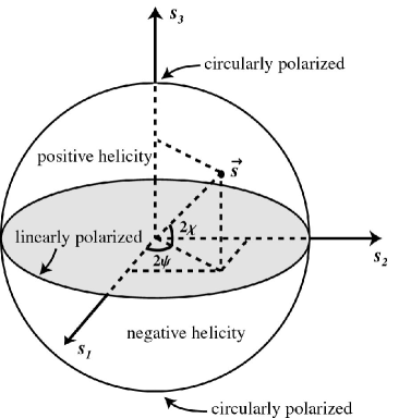
FIG. 2.: The Poincaré sphere.

In Sec. III C, the quantity of interest is the polarization change induced by the phase shift $\Delta\phi$ in Eq. (47). The effect of $\Delta\phi$ on the Stokes vector $\vec{s}$ can be visualized in terms of motion on the Poincaré sphere. Consider an arbitrary orthonormal elliptical basis $\{\hat{\varepsilon}_{1},\hat{\varepsilon}_{2}\}$. The associated Stokes vectors $\vec{s}_{\hat{\varepsilon}_{1}}$, $\vec{s}_{\hat{\varepsilon}_{2}}$ determine opposite points on the Poincaré sphere. Decomposing a general electric field in this basis gives polarization components $E_{n}e^{-i\phi_{n}}$, $n=1,2$, where $E_{n}$ and $\phi_{n}$ are real. Examining the Stokes vector for this configuration shows that a change $\Delta(\phi_{1}-\phi_{2})$ in the relative phase results in a right-handed rotation of the Stokes vector by the angle $\Delta(\phi_{1}-\phi_{2})$ about the axis given by $\vec{s}_{\hat{\varepsilon}_{1}}=-\vec{s}_{\hat{\varepsilon}_{2}}$.

C Standard Frames

This appendix defines our standard frames for Earth- and space-based laboratories. We provide the rotations and velocities used in transforming to the reference Sun-centered celestial equatorial frame, which is defined in section III A.

1 Earth-based laboratory

For a laboratory fixed to the surface of the Earth in the northern hemisphere, we choose the standard frame to have coordinates $(t,x,y,z)$ such that the $x$-axis points south, the $y$-axis points east, and the $z$-axis points vertically upwards. With the reasonable approximation that the orbit of the Earth is circular, the rotation from the Sun-centered celestial equatorial frame to the standard laboratory frame is given by

$$R^{jJ}=\left(\begin{array}[]{ccc}\cos\chi\cos\omega_{\oplus}T_{\oplus}&\cos\chi\sin\omega_{\oplus}T_{\oplus}&-\sin\chi\\ -\sin\omega_{\oplus}T_{\oplus}&\cos\omega_{\oplus}T_{\oplus}&0\\ \sin\chi\cos\omega_{\oplus}T_{\oplus}&\sin\chi\sin\omega_{\oplus}T_{\oplus}&\cos\chi\end{array}\right).$$ (C1)

In this equation, $j=$ $x,y,z$ $=1,2,3$ denotes an index in the laboratory frame, while $J=X$, $Y$, $Z$ denotes an index in the Sun-centered frame. The Earth’s sidereal angular frequency is $\omega_{\oplus}\simeq 2\pi$/(23 h 56 min.), and $\chi$ is the colatitude of the laboratory. The time $T_{\oplus}$ is measured in the Sun-centered frame from one of the times when the $y$- and $Y$-axes coincide, to be chosen conveniently for each experiment. The time $T_{\oplus}$ therefore differs from the celestial equatorial time $T$ by a constant shift for each experiment.

The velocity 3-vector of the laboratory in the Sun-centered frame is

$$\vec{\beta}=\beta_{\oplus}\left(\begin{array}[]{c}\sin\Omega_{\oplus}T\\ -\cos\eta\cos\Omega_{\oplus}T\\ -\sin\eta\cos\Omega_{\oplus}T\end{array}\right)+\beta_{L}\left(\begin{array}[]{c}-\sin\omega_{\oplus}T_{\oplus}\\ \cos\omega_{\oplus}T_{\oplus}\\ 0\end{array}\right)\ .$$ (C2)

Here, $\Omega_{\oplus}$ and $\beta_{\oplus}$ are, respectively, the angular frequency and speed of the Earth’s orbital motion. The quantity $\eta\simeq 23.4^{\circ}$ is the angle between the $XY$ celestial equatorial plane and the Earth’s orbital plane. The speed $\beta_{L}=r_{\oplus}\omega_{\oplus}\sin\chi\mathrel{\hbox to0.0pt{\lower 4.0pt\hbox{\hskip 1.0pt$\sim$}\hss}\raise 1.0pt\hbox{$<$}}1.5\times 10^{-6}$ is that of the laboratory due to the rotation of the Earth.

The reader is warned that the standard laboratory frame defined above may differ from a frame fixed to the apparatus in the laboratory. For example, the apparatus rotates in the laboratory in some experiments considered here. Where confusion could occur, we distinguish with labels the quantities defined in the standard laboratory frame from those in the apparatus frame.

2 Space-based laboratory

For our standard laboratory fixed to an Earth-orbiting space platform such as the ISS, we choose the $z$ axis to be aligned with the velocity $\vec{\beta}_{s}$ of the satellite with respect to the Earth. The $x$ axis is chosen to point towards the Earth. The $y$ axis completes a right-handed coordinate system, thus directed along the satellite orbital angular momentum with respect to the Earth.

The components of the matrix $R^{jJ}$ describing the rotation from the reference Sun-centered frame to this standard satellite frame are

$$R^{1X} = -\cos\alpha\cos\omega_{s}T_{s}+\sin\alpha\cos\zeta\sin\omega_{s}T_{s},$$ (C3)

$$R^{1Y} = -\sin\alpha\cos\omega_{s}T_{s}-\cos\alpha\cos\zeta\sin\omega_{s}T_{s},$$ (C4)

$$R^{1Z} = -\sin\zeta\sin\omega_{s}T_{s},$$ (C5)

$$R^{2X} = \sin\alpha\sin\zeta,$$ (C6)

$$R^{2Y} = -\cos\alpha\sin\zeta,$$ (C7)

$$R^{2Z} = \cos\zeta,$$ (C8)

$$R^{3X} = -\cos\alpha\sin\omega_{s}T_{s}-\sin\alpha\cos\zeta\cos\omega_{s}T_{s},$$ (C9)

$$R^{3Y} = -\sin\alpha\sin\omega_{s}T_{s}+\cos\alpha\cos\zeta\cos\omega_{s}T_{s},$$ (C10)

$$R^{3Z} = \sin\zeta\cos\omega_{s}T_{s}.$$ (C11)

Here, $j=1,2,3$ denotes an index in the satellite frame. The satellite orbital angular frequency is denoted $\omega_{s}$. The time $T_{s}$ is measured in the Sun-centered frame from a conveniently chosen time when the satellite crosses the equatorial plane, so the times $T_{s}$ and $T$ differ by a constant for each experiment. Also, $\zeta$ is the angle between the satellite orbital plane and the Earth’s equatorial plane. For example, $\zeta\simeq 52^{\circ}$ for the ISS. The quantity $\alpha$ is the azimuthal angle at which the orbital plane intersects the Earth’s equatorial plane. The satellite intersects the equatorial plane twice per orbit, and $\alpha$ can be regarded as the angle between the $X$ direction and a vector from the Earth’s center to the point where the intersection occurs on an ascending trajectory.

The velocity of the satellite with respect to the Sun-centered celestial equatorial frame is

$$\vec{\beta} = \beta_{\oplus}\left(\begin{array}[]{c}\sin\Omega_{\oplus}T\\ -\cos\eta\cos\Omega_{\oplus}T\\ -\sin\eta\cos\Omega_{\oplus}T\end{array}\right)$$ (C19)

$$\hskip-7.0pt+\beta_{s}\left(\begin{array}[]{c}-\cos\alpha\sin\omega_{s}T_{s}-\sin\alpha\cos\zeta\cos\omega_{s}T_{s}\\ -\sin\alpha\sin\omega_{s}T_{s}+\cos\alpha\cos\zeta\cos\omega_{s}T_{s}\\ \sin\zeta\cos\omega_{s}T_{s}\end{array}\right).$$

The quantities $\beta_{\oplus}$, $\Omega_{\oplus}$ are defined as before. The quantity $\beta_{s}$ is the speed of the satellite with respect to the Earth. For example, $\beta_{s}\simeq 3\times 10^{-5}$ for the ISS.

D Optical frequency shift

This appendix provides an alternative method to obtain the fractional resonant-frequency shift $\delta\nu/\nu$ for optical cavities, given in Eq. (70). As before, the cavity is regarded as two reflecting parallel planar surfaces separated by a distance $l$. For convenience, we let one coincide with the $x$-$y$ plane and place the other at $z=l$. We approximate the light entering the cavity as a plane wave with phase velocity parallel to the $z$-axis. After each reflection inside the cavity, the reflected wave must have the same frequency as the incident wave, so we consider light of constant frequency $p^{0}$. For simplicity, we set $\epsilon=1$ in what follows.

At leading order in the coefficients for Lorentz violation, Eq. (40) implies that the magnitude of the wave vector for each birefringent mode is $|\vec{p}_{\pm}|=p_{\pm}=[1-(\rho\pm\sigma)]p^{0}$. Decomposing the light entering the cavity into birefringent modes, we write

$$\vec{E}_{0}(x) = e^{-ip^{0}t}[e^{ip_{\uparrow+}z}(\hat{\varepsilon}_{\uparrow+}\cdot\vec{E}_{0})\hat{\varepsilon}_{\uparrow+}$$ (D2)

$$\qquad\quad+e^{ip_{\uparrow-}z}(\hat{\varepsilon}_{\uparrow-}\cdot\vec{E}_{0})\hat{\varepsilon}_{\uparrow-}].$$

Here, $p_{\uparrow\pm}=[1-(\rho_{\uparrow}\pm\sigma_{\uparrow})]p^{0}$, where $\rho_{\uparrow}$ and $\sigma_{\uparrow}$ denote the values of $\rho$ and $\sigma$ for light with phase velocity in the $z$ direction. The unit vectors $\hat{\varepsilon}_{\uparrow\pm}$ are the associated birefringent basis.

We suppose that the wave reflected at $z=l$ has phase velocity in the $-z$ direction. Decomposing this wave in the same fashion gives

$$\vec{E}_{1}(x) = e^{-ip^{0}t}\bigl{(}e^{-ip_{\downarrow+}z}(\hat{\varepsilon}_{\downarrow+}\cdot\vec{E}_{1})\hat{\varepsilon}_{\downarrow+}$$ (D4)

$$\qquad\quad+e^{-ip_{\downarrow-}z}(\hat{\varepsilon}_{\downarrow-}\cdot\vec{E}_{1})\hat{\varepsilon}_{\downarrow-}\bigr{)},$$

where the subscript $\downarrow$ denotes quantities for phase velocity in the $-z$ direction. Similar expressions can be written for the electric field $\vec{E}_{n}(x)$ after $n$ reflections. For the $n$th reflection with $n$ odd, the incident and reflected waves are related by $\vec{E}_{n+1}(x)|_{z=l}=e^{i\delta_{l,n}}\vec{E}_{n}(x)|_{z=l}$. A similar relation involving $\delta_{0,n}$ holds for even $n$ at $z=0$. The complex factors $e^{i\delta_{0,n}}$, $e^{i\delta_{l,n}}$ account for any phase change or loss due to transmission or absorption. They may depend on the interaction of the wave with the surfaces and could also depend on the incident polarization and various coefficients for Lorentz violation. For simplicity, we suppose here that they are constant, and denote them by $\delta_{0}$ and $\delta_{l}$.

Superposing the contributions inside the cavity yields the total electric field as

$$\vec{E}(x) = e^{-ip^{0}t}[(e^{ip_{\uparrow+}z}\hat{\varepsilon}_{\uparrow+}\hat{\varepsilon}_{\uparrow+}^{\dagger}+e^{ip_{\uparrow-}z}\hat{\varepsilon}_{\uparrow-}\hat{\varepsilon}_{\uparrow-}^{\dagger})$$ (D6)

$$\hskip-30.0pt+e^{-i\delta_{0}}(e^{-ip_{\downarrow+}z}\hat{\varepsilon}_{\downarrow+}\hat{\varepsilon}_{\downarrow+}^{\dagger}+e^{-ip_{\downarrow-}z}\hat{\varepsilon}_{\downarrow-}\hat{\varepsilon}_{\downarrow-}^{\dagger})m]\cdot M\cdot\vec{E}_{0}.$$

At leading order, the matrix $m$ is given by

$$m = e^{i(2p^{0}l+\delta_{0}+\delta_{l})}$$ (D8)

$$\times \left[1-i2p^{0}l\left(\begin{array}[]{ccc}\overline{\rho+\sigma\cos\xi}&\overline{\sigma\sin\xi}&0\\ \overline{\sigma\sin\xi}&\overline{\rho-\sigma\cos\xi}&0\\ 0&0&0\end{array}\right)\right]\ ,$$ (D12)

where the bar signifies the average value over the two different propagation directions. The matrix $M$ is the geometric series $M=\sum_{n=0}^{\infty}m^{n}=(1-m)^{-1}$.

The resonant frequency is often viewed as the frequency at which a standing wave is produced in the cavity. However, this notion may fail for nonzero $k_{F}$ because the wavelength of light traveling in one direction can differ from that for light traveling in the opposite direction. A more appropriate definition that applies also in the conventional case is to take the resonant frequency as the frequency maximizing the magnitude of the electric field or the energy density. The resonant frequency for a cavity is determined experimentally by measuring the transmitted light, so we adopt the energy density of the transmitted light as the relevant quantity. Using instead the magnitude of the transmitted electric or magnetic field yields the same result at leading order.

We assume that the electric field $\vec{E}_{T}$ of the transmitted light is proportional to the component of the total electric field in the cavity propagating in the $z$ direction:

$$\vec{E}_{T}\propto e^{-ip^{0}t}(e^{ip_{\uparrow+}z}\hat{\varepsilon}_{\uparrow+}\hat{\varepsilon}_{\uparrow+}^{\dagger}+e^{ip_{\uparrow-}z}\hat{\varepsilon}_{\uparrow-}\hat{\varepsilon}_{\uparrow-}^{\dagger})\cdot M\cdot\vec{E}_{0}.$$ (D13)

The time-averaged energy density is

$$\langle{u}\rangle = {\textstyle{{1}\over{4}}}\hbox{Re}\,(\vec{E}^{*}\cdot\vec{D}+\vec{B}^{*}\cdot\vec{H})$$ (D14)

$$= {\textstyle{{1}\over{4}}}[\vec{E}^{*}\cdot(1+\kappa_{DE})\cdot\vec{E}+\vec{B}^{*}\cdot(1+\kappa_{HB})\cdot\vec{B}].$$ (D15)

With this equation and the Faraday law $ip^{0}\vec{B}=\vec{\nabla}\times\vec{E}$, the energy density of the transmitted wave can be calculated. Maximizing with respect to $p^{0}$ and solving for $p^{0}$ yields the perturbed resonant frequency. We find

$${{\delta\nu}\over{\nu}}={{\vec{E}_{0}^{*}}\over{|\vec{E}_{0}|}}\cdot\left(\begin{array}[]{ccc}\overline{\rho+\sigma\cos\xi}&\overline{\sigma\sin\xi}&0\\ \overline{\sigma\sin\xi}&\overline{\rho-\sigma\cos\xi}&0\\ 0&0&0\end{array}\right)\cdot{{\vec{E}_{0}}\over{|\vec{E}_{0}|}}\ .$$ (D16)

The barred quantities can be determined from

$$\rho = -{\textstyle{1\over 2}}(\tilde{\kappa}_{e-})^{11}-{\textstyle{1\over 2}}(\tilde{\kappa}_{e-})^{22}-(\tilde{\kappa}_{o+})^{12}-\tilde{\kappa}_{\rm tr},$$ (D17)

$$\sigma\sin\xi = {\textstyle{1\over 2}}(\tilde{\kappa}_{o-})^{11}-{\textstyle{1\over 2}}(\tilde{\kappa}_{o-})^{22}-(\tilde{\kappa}_{e+})^{12},$$ (D18)

$$\sigma\cos\xi = -{\textstyle{1\over 2}}(\tilde{\kappa}_{e+})^{11}+{\textstyle{1\over 2}}(\tilde{\kappa}_{e+})^{22}-(\tilde{\kappa}_{o-})^{12},$$ (D19)

which holds for a wave traveling in the $+z$ direction. For a wave traveling in the $-z$ direction, one must instead use Eq. (D19) with sign changes for the parity-odd coefficients: $\kappa_{DB}\rightarrow-\kappa_{DB}$, $\kappa_{HE}\rightarrow-\kappa_{HE}$. The barred quantities in Eq. (62) then are merely those in (D19) with $\kappa_{DB}=\kappa_{HE}=0$. The net result is Eq. (70), as desired.

E Laboratory-frame quantities

In the scenario of Sec. IV B 1 and in terms of the matrices $\tilde{\kappa}$ introduced in Eq. (15), the quantities $A_{0,1,2,3,4}$ defined in Eq. (83) can be written as

$$A_{0} = {\textstyle{{1}\over{8}}}(1-3\cos^{2}\chi)[3\epsilon_{+}(\tilde{\kappa}_{e+})^{ZZ}+\epsilon_{-}(\tilde{\kappa}_{e-})^{ZZ}]$$ (E8)

$$-{\textstyle{{1}\over{8}}}(9\epsilon_{+}-\epsilon_{-})\tilde{\kappa}_{\rm tr}$$

$$+{\textstyle{{1}\over{4}}}\beta_{\oplus}\bigl{[}2\bigl{(}\epsilon_{-}-3\epsilon_{+}\cos^{2}\chi\bigr{)}\sin\eta\cos\Omega_{\oplus}T(\tilde{\kappa}_{o+})^{XY}$$

$$+\bigl{(}3\epsilon_{+}-2\epsilon_{-}-3\epsilon_{+}\cos^{2}\chi\bigr{)}$$

$$\times\bigl{(}\cos\eta\cos\Omega_{\oplus}T(\tilde{\kappa}_{o+})^{XZ}+\sin\Omega_{\oplus}T(\tilde{\kappa}_{o+})^{YZ}\bigr{)}$$

$$-3\epsilon_{+}(1-3\cos^{2}\chi)$$

$$\times\bigl{(}\cos\eta\cos\Omega_{\oplus}T(\tilde{\kappa}_{o-})^{XZ}+\sin\Omega_{\oplus}T(\tilde{\kappa}_{o-})^{YZ}\bigr{)}\bigr{]}$$

$$+{\textstyle{{9}\over{4}}}\epsilon_{+}\beta_{L}\sin\chi\cos\chi(\tilde{\kappa}_{o-})^{ZZ},$$

$$A_{1} = -{\textstyle{{1}\over{2}}}\sin\chi\cos\chi[3\epsilon_{+}(\tilde{\kappa}_{e+})^{YZ}+\epsilon_{-}(\tilde{\kappa}_{e-})^{YZ}]$$ (E14)

$$+{\textstyle{{3}\over{2}}}\epsilon_{+}\beta_{\oplus}\sin\chi\cos\chi[\sin\Omega_{\oplus}T((\tilde{\kappa}_{o-})^{YY}-(\tilde{\kappa}_{o-})^{ZZ})$$

$$-\cos\eta\cos\Omega_{\oplus}T((\tilde{\kappa}_{o+})^{XY}-(\tilde{\kappa}_{o-})^{XY})$$

$$+\sin\eta\cos\Omega_{\oplus}T((\tilde{\kappa}_{o+})^{XZ}-(\tilde{\kappa}_{o-})^{XZ})]$$

$$+{\textstyle{{1}\over{2}}}\beta_{L}[\epsilon_{-}(\tilde{\kappa}_{o+})^{YZ}$$

$$+3\epsilon_{+}(\sin^{2}\chi-\cos^{2}\chi)(\tilde{\kappa}_{o-})^{YZ}],$$

$$A_{2} = -{\textstyle{{1}\over{2}}}\sin\chi\cos\chi[3\epsilon_{+}(\tilde{\kappa}_{e+})^{XZ}+\epsilon_{-}(\tilde{\kappa}_{e-})^{XZ}]$$ (E20)

$$+{\textstyle{{3}\over{2}}}\epsilon_{+}\beta_{\oplus}\sin\chi\cos\chi[\sin\Omega_{\oplus}T((\tilde{\kappa}_{o+})^{XY}+(\tilde{\kappa}_{o-})^{XY})$$

$$+\cos\eta\cos\Omega_{\oplus}T((\tilde{\kappa}_{o-})^{XX}-(\tilde{\kappa}_{o-})^{ZZ})$$

$$-\sin\eta\cos\Omega_{\oplus}T((\tilde{\kappa}_{o+})^{YZ}-(\tilde{\kappa}_{o-})^{YZ})]$$

$$+{\textstyle{{1}\over{2}}}\beta_{L}[\epsilon_{-}(\tilde{\kappa}_{o+})^{XZ}$$

$$+3\epsilon_{+}(\sin^{2}\chi-\cos^{2}\chi)(\tilde{\kappa}_{o-})^{XZ}],$$

$$A_{3} = -{\textstyle{{1}\over{4}}}\sin^{2}\chi[3\epsilon_{+}(\tilde{\kappa}_{e+})^{XY}+\epsilon_{-}(\tilde{\kappa}_{e-})^{XY}]$$ (E25)

$$-{\textstyle{{3}\over{4}}}\epsilon_{+}\beta_{\oplus}\sin^{2}\chi[\sin\Omega_{\oplus}T((\tilde{\kappa}_{o+})^{XZ}+(\tilde{\kappa}_{o-})^{XZ})$$

$$+\cos\eta\cos\Omega_{\oplus}T((\tilde{\kappa}_{o+})^{YZ}+(\tilde{\kappa}_{o-})^{YZ})$$

$$+\sin\eta\cos\Omega_{\oplus}T((\tilde{\kappa}_{o-})^{XX}-(\tilde{\kappa}_{o-})^{YY})]$$

$$-{\textstyle{{3}\over{2}}}\epsilon_{+}\beta_{L}\sin\chi\cos\chi(\tilde{\kappa}_{o-})^{XY},$$

$$A_{4} = -{\textstyle{{1}\over{8}}}\sin^{2}\chi\bigl{[}3\epsilon_{+}\bigl{(}(\tilde{\kappa}_{e+})^{XX}-(\tilde{\kappa}_{e+})^{YY}\bigr{)}$$ (E31)

$$+\epsilon_{-}\bigl{(}(\tilde{\kappa}_{e-})^{XX}-(\tilde{\kappa}_{e-})^{YY}\bigr{)}\bigr{]}$$

$$+{\textstyle{{3}\over{4}}}\epsilon_{+}\beta_{\oplus}\sin^{2}\chi[\sin\Omega_{\oplus}T((\tilde{\kappa}_{o+})^{YZ}+(\tilde{\kappa}_{o-})^{YZ})$$

$$-\cos\eta\cos\Omega_{\oplus}T((\tilde{\kappa}_{o+})^{XZ}+(\tilde{\kappa}_{o-})^{XZ})$$

$$+2\sin\eta\cos\Omega_{\oplus}T(\tilde{\kappa}_{o-})^{XY}]$$

$$-{\textstyle{{3}\over{4}}}\epsilon_{+}\beta_{L}\sin\chi\cos\chi[(\tilde{\kappa}_{o-})^{XX}-(\tilde{\kappa}_{o-})^{YY}].$$

In this equation, we have introduced the quantities

$$\epsilon_{+}={{2+\epsilon}\over{3\epsilon}},\quad\epsilon_{-}={{2-\epsilon}\over{\epsilon}},$$ (E32)

which both reduce to 1 in the vacuum limit $\epsilon\to 1$.

The remaining coefficients are independent of $\epsilon$. The coefficients $B_{0,1,2,3,4}$ are given by

$$B_{0} = -{\textstyle{1\over 2}}\beta_{L}\sin\chi(\tilde{\kappa}_{o+})^{XY},$$ (E33)

$$B_{1} = -{\textstyle{1\over 2}}\sin\chi[(\tilde{\kappa}_{e+})^{XZ}-(\tilde{\kappa}_{e-})^{XZ}]$$ (E38)

$$+{\textstyle{1\over 2}}\beta_{\oplus}\sin\chi[\sin\Omega_{\oplus}T((\tilde{\kappa}_{o+})^{XY}+(\tilde{\kappa}_{o-})^{XY})$$

$$+\cos\eta\cos\Omega_{\oplus}T((\tilde{\kappa}_{o-})^{XX}-(\tilde{\kappa}_{o-})^{ZZ})$$

$$-\sin\eta\cos\Omega_{\oplus}T((\tilde{\kappa}_{o+})^{YZ}-(\tilde{\kappa}_{o-})^{YZ})]$$

$$-{\textstyle{1\over 2}}\beta_{L}\cos\chi((\tilde{\kappa}_{o+})^{XZ}+(\tilde{\kappa}_{o-})^{XZ}),$$

$$B_{2} = {\textstyle{1\over 2}}\sin\chi[(\tilde{\kappa}_{e+})^{YZ}-(\tilde{\kappa}_{e-})^{YZ}]$$ (E43)

$$-{\textstyle{1\over 2}}\beta_{\oplus}\sin\chi[\sin\Omega_{\oplus}T((\tilde{\kappa}_{o-})^{YY}-(\tilde{\kappa}_{o-})^{ZZ})$$

$$-\cos\eta\cos\Omega_{\oplus}T((\tilde{\kappa}_{o+})^{XY}-(\tilde{\kappa}_{o-})^{XY})$$

$$+\sin\eta\cos\Omega_{\oplus}T((\tilde{\kappa}_{o+})^{XZ}-(\tilde{\kappa}_{o-})^{XZ})]$$

$$+{\textstyle{1\over 2}}\beta_{L}\cos\chi((\tilde{\kappa}_{o+})^{YZ}+(\tilde{\kappa}_{o-})^{YZ}),$$

$$B_{3} = {\textstyle{{1}\over{4}}}\cos\chi[(\tilde{\kappa}_{e+})^{XX}-(\tilde{\kappa}_{e-})^{XX}$$ (E49)

$$-(\tilde{\kappa}_{e+})^{YY}+(\tilde{\kappa}_{e-})^{YY}]$$

$$-{\textstyle{1\over 2}}\beta_{\oplus}\cos\chi[\sin\Omega_{\oplus}T((\tilde{\kappa}_{o+})^{YZ}+(\tilde{\kappa}_{o-})^{YZ})$$

$$-\cos\eta\cos\Omega_{\oplus}T((\tilde{\kappa}_{o+})^{XZ}+(\tilde{\kappa}_{o-})^{XZ})$$

$$+2\sin\eta\cos\Omega_{\oplus}T(\tilde{\kappa}_{o-})^{XY}]$$

$$-{\textstyle{{1}\over{4}}}\beta_{L}\sin\chi[(\tilde{\kappa}_{o-})^{XX}-(\tilde{\kappa}_{o-})^{YY}],$$

$$B_{4} = -{\textstyle{1\over 2}}\cos\chi[(\tilde{\kappa}_{e+})^{XY}-(\tilde{\kappa}_{e-})^{XY}]$$ (E54)

$$-{\textstyle{1\over 2}}\beta_{\oplus}\cos\chi[\sin\Omega_{\oplus}T((\tilde{\kappa}_{o+})^{XZ}+(\tilde{\kappa}_{o-})^{XZ})$$

$$+\cos\eta\cos\Omega_{\oplus}T((\tilde{\kappa}_{o+})^{YZ}+(\tilde{\kappa}_{o-})^{YZ})$$

$$+\sin\eta\cos\Omega_{\oplus}T((\tilde{\kappa}_{o-})^{XX}-(\tilde{\kappa}_{o-})^{YY})]$$

$$+{\textstyle{1\over 2}}\beta_{L}\sin\chi(\tilde{\kappa}_{o-})^{XY}.$$

The coefficients $C_{0,1,2,3,4}$ are

$$C_{0} = -{\textstyle{{3}\over{8}}}\sin^{2}\chi[(\tilde{\kappa}_{e+})^{ZZ}-(\tilde{\kappa}_{e-})^{ZZ}]$$ (E59)

$$-{\textstyle{{1}\over{4}}}\beta_{\oplus}\sin^{2}\chi[\sin\Omega_{\oplus}T((\tilde{\kappa}_{o+})^{YZ}-3(\tilde{\kappa}_{o-})^{YZ})$$

$$+\cos\eta\cos\Omega_{\oplus}T((\tilde{\kappa}_{o+})^{XZ}-3(\tilde{\kappa}_{o-})^{XZ})$$

$$+2\sin\eta\cos\Omega_{\oplus}T(\tilde{\kappa}_{o+})^{XY}]$$

$$-{\textstyle{{3}\over{4}}}\beta_{L}\sin\chi\cos\chi(\tilde{\kappa}_{o-})^{ZZ},$$

$$C_{1} = {\textstyle{1\over 2}}\sin\chi\cos\chi[(\tilde{\kappa}_{e+})^{YZ}-(\tilde{\kappa}_{e-})^{YZ}]$$ (E64)

$$-{\textstyle{1\over 2}}\beta_{\oplus}\sin\chi\cos\chi[\sin\Omega_{\oplus}T((\tilde{\kappa}_{o-})^{YY}-(\tilde{\kappa}_{o-})^{ZZ})$$

$$-\cos\eta\cos\Omega_{\oplus}T((\tilde{\kappa}_{o+})^{XY}-(\tilde{\kappa}_{o-})^{XY})$$

$$+\sin\eta\cos\Omega_{\oplus}T((\tilde{\kappa}_{o+})^{XZ}-(\tilde{\kappa}_{o-})^{XZ})]$$

$$+{\textstyle{1\over 2}}\beta_{L}[(\tilde{\kappa}_{o+})^{YZ}-(\sin^{2}\chi-\cos^{2}\chi)(\tilde{\kappa}_{o-})^{YZ}],$$

$$C_{2} = {\textstyle{1\over 2}}\sin\chi\cos\chi[(\tilde{\kappa}_{e+})^{XZ}-(\tilde{\kappa}_{e-})^{XZ}]$$ (E69)

$$-{\textstyle{1\over 2}}\beta_{\oplus}\sin\chi\cos\chi[\sin\Omega_{\oplus}T((\tilde{\kappa}_{o+})^{XY}+(\tilde{\kappa}_{o-})^{XY})$$

$$+\cos\eta\cos\Omega_{\oplus}T((\tilde{\kappa}_{o-})^{XX}-(\tilde{\kappa}_{o-})^{ZZ})$$

$$-\sin\eta\cos\Omega_{\oplus}T((\tilde{\kappa}_{o+})^{YZ}-(\tilde{\kappa}_{o-})^{YZ})]$$

$$+{\textstyle{1\over 2}}\beta_{L}[(\tilde{\kappa}_{o+})^{XZ}-(\sin^{2}\chi-\cos^{2}\chi)(\tilde{\kappa}_{o-})^{XZ}],$$

$$C_{3} = -{\textstyle{{1}\over{4}}}(1+\cos^{2}\chi)[(\tilde{\kappa}_{e+})^{XY}-(\tilde{\kappa}_{e-})^{XY}]$$ (E74)

$$-{\textstyle{{1}\over{4}}}\beta_{\oplus}(1+\cos^{2}\chi)[\sin\Omega_{\oplus}T((\tilde{\kappa}_{o+})^{XZ}+(\tilde{\kappa}_{o-})^{XZ})$$

$$+\cos\eta\cos\Omega_{\oplus}T((\tilde{\kappa}_{o+})^{YZ}+(\tilde{\kappa}_{o-})^{YZ})$$

$$+\sin\eta\cos\Omega_{\oplus}T((\tilde{\kappa}_{o-})^{XX}-(\tilde{\kappa}_{o-})^{YY})]$$

$$+{\textstyle{1\over 2}}\beta_{L}\sin\chi\cos\chi(\tilde{\kappa}_{o-})^{XY},$$

$$C_{4} = -{\textstyle{{1}\over{8}}}(1+\cos^{2}\chi)[(\tilde{\kappa}_{e+})^{XX}-(\tilde{\kappa}_{e-})^{XX}$$ (E80)

$$-(\tilde{\kappa}_{e+})^{YY}+(\tilde{\kappa}_{e-})^{YY}]$$

$$+{\textstyle{{1}\over{4}}}\beta_{\oplus}(1+\cos^{2}\chi)[\sin\Omega_{\oplus}T((\tilde{\kappa}_{o+})^{YZ}+(\tilde{\kappa}_{o-})^{YZ})$$

$$-\cos\eta\cos\Omega_{\oplus}T((\tilde{\kappa}_{o+})^{XZ}+(\tilde{\kappa}_{o-})^{XZ})$$

$$+2\sin\eta\cos\Omega_{\oplus}T(\tilde{\kappa}_{o-})^{XY}]$$

$$+{\textstyle{{1}\over{4}}}\beta_{L}\sin\chi\cos\chi[(\tilde{\kappa}_{o-})^{XX}-(\tilde{\kappa}_{o-})^{YY}].$$

F Satellite-frame quantities

The quantities ${\cal A}_{s,c}$, ${\cal B}_{s,c}$ appearing in Eq. (119) of Sec. IV C 2 can be expressed in terms of the matrices $\tilde{\kappa}$ introduced in Eq. (15) through the convenient combinations (111). In terms of the various orientation angles specified in Appendix C, for the quantity ${\cal A}_{s}$ we find

$${\cal A}_{s} = {\textstyle{{1}\over{4}}}\cos 2\zeta[\sin\alpha(\tilde{\kappa}_{e^{\prime}})^{XZ}-\cos\alpha(\tilde{\kappa}_{e^{\prime}})^{YZ}]$$ (F20)

$$+{\textstyle{{1}\over{8}}}\sin 2\zeta[(1+\sin^{2}\alpha)(\tilde{\kappa}_{e^{\prime}})^{XX}$$

$$+(1+\cos^{2}\alpha)(\tilde{\kappa}_{e^{\prime}})^{YY}-\sin 2\alpha(\tilde{\kappa}_{e^{\prime}})^{XY}]$$

$$+{\textstyle{{1}\over{4}}}\beta_{s}\bigl{[}\sin\alpha\bigl{(}(\tilde{\kappa}_{o^{\prime}})^{XZ}-(\tilde{\kappa}_{o^{\prime}})^{ZX}\bigr{)}$$

$$-\cos\alpha\bigl{(}(\tilde{\kappa}_{o^{\prime}})^{YZ}-(\tilde{\kappa}_{o^{\prime}})^{ZY}\bigr{)}\bigr{]}$$

$$+{\textstyle{{1}\over{4}}}\beta_{\oplus}\bigl{[}\cos\alpha\cos 2\zeta\cos\Omega_{\oplus}T$$

$$\times\bigl{(}\cos\eta(\tilde{\kappa}_{o^{\prime}})^{YX}-\sin\eta(\tilde{\kappa}_{o^{\prime}})^{ZX}\bigr{)}$$

$$+\cos\alpha\cos 2\zeta\sin\Omega_{\oplus}T\bigl{(}(\tilde{\kappa}_{o^{\prime}})^{YY}-(\tilde{\kappa}_{o^{\prime}})^{ZZ}\bigr{)}$$

$$-\sin\alpha\cos 2\zeta\cos\Omega_{\oplus}T$$

$$\times\bigl{(}\cos\eta\bigl{(}(\tilde{\kappa}_{o^{\prime}})^{XX}-(\tilde{\kappa}_{o^{\prime}})^{ZZ}\bigr{)}+\sin\eta(\tilde{\kappa}_{o^{\prime}})^{ZY}\bigr{)}$$

$$-\sin\alpha\cos 2\zeta\sin\Omega_{\oplus}T(\tilde{\kappa}_{o^{\prime}})^{XY}$$

$$+\cos^{2}\alpha\sin 2\zeta\cos\Omega_{\oplus}T$$

$$\times\bigl{(}\cos\eta(\tilde{\kappa}_{o^{\prime}})^{ZX}+\sin\eta(\tilde{\kappa}_{o^{\prime}})^{YX}\bigr{)}$$

$$+\cos^{2}\alpha\sin 2\zeta\sin\Omega_{\oplus}T\bigl{(}(\tilde{\kappa}_{o^{\prime}})^{YZ}+(\tilde{\kappa}_{o^{\prime}})^{ZY}\bigr{)}$$

$$+\sin^{2}\alpha\sin 2\zeta\cos\Omega_{\oplus}T$$

$$\times\bigl{(}\cos\eta\bigl{(}(\tilde{\kappa}_{o^{\prime}})^{XZ}+(\tilde{\kappa}_{o^{\prime}})^{ZX}\bigr{)}-\sin\eta(\tilde{\kappa}_{o^{\prime}})^{XY}\bigr{)}$$

$$+\sin^{2}\alpha\sin 2\zeta\sin\Omega_{\oplus}T(\tilde{\kappa}_{o^{\prime}})^{ZY}$$

$$-{\textstyle{1\over 2}}\sin 2\alpha\sin 2\zeta\cos\Omega_{\oplus}T$$

$$\times\bigl{(}\cos\eta(\tilde{\kappa}_{o^{\prime}})^{YZ}+\sin\eta\bigl{(}(\tilde{\kappa}_{o^{\prime}})^{XX}-(\tilde{\kappa}_{o^{\prime}})^{YY}\bigr{)}\bigr{)}$$

$$-{\textstyle{1\over 2}}\sin 2\alpha\sin 2\zeta\sin\Omega_{\oplus}T(\tilde{\kappa}_{o^{\prime}})^{XZ}\bigr{]}.$$

The quantity ${\cal A}_{c}$ is

$${\cal A}_{c} = -{\textstyle{{1}\over{4}}}\cos\zeta\sin\alpha(\tilde{\kappa}_{e^{\prime}})^{YZ}$$ (F39)

$$-{\textstyle{{1}\over{4}}}\cos\zeta\cos\alpha(\tilde{\kappa}_{e^{\prime}})^{XZ}$$

$$-{\textstyle{{1}\over{8}}}\sin\zeta\sin 2\alpha\bigl{(}(\tilde{\kappa}_{e^{\prime}})^{XX}-(\tilde{\kappa}_{e^{\prime}})^{YY}\bigr{)}$$

$$+{\textstyle{{1}\over{4}}}\sin\zeta\cos 2\alpha(\tilde{\kappa}_{e^{\prime}})^{XY}$$

$$+{\textstyle{{1}\over{4}}}\beta_{s}\bigl{[}\sin\zeta\bigl{(}(\tilde{\kappa}_{o^{\prime}})^{XY}-(\tilde{\kappa}_{o^{\prime}})^{YX}\bigr{)}$$

$$+\cos\zeta\cos\alpha\bigl{(}(\tilde{\kappa}_{o^{\prime}})^{ZX}-(\tilde{\kappa}_{o^{\prime}})^{XZ}\bigr{)}$$

$$+\cos\zeta\sin\alpha\bigl{(}(\tilde{\kappa}_{o^{\prime}})^{ZY}-(\tilde{\kappa}_{o^{\prime}})^{YZ}\bigr{)}\bigr{]}$$

$$+{\textstyle{{1}\over{4}}}\beta_{\oplus}\bigl{[}\cos\alpha\cos\zeta\cos\Omega_{\oplus}T$$

$$\times\bigl{(}\cos\eta\bigl{(}(\tilde{\kappa}_{o^{\prime}})^{XX}-(\tilde{\kappa}_{o^{\prime}})^{ZZ}\bigr{)}+\sin\eta(\tilde{\kappa}_{o^{\prime}})^{ZY}\bigr{)}$$

$$+\cos\alpha\cos\zeta\sin\Omega_{\oplus}T(\tilde{\kappa}_{o^{\prime}})^{XY}$$

$$+\sin\alpha\cos\zeta\cos\Omega_{\oplus}T$$

$$\times\bigl{(}\cos\eta(\tilde{\kappa}_{o^{\prime}})^{YX}-\sin\eta(\tilde{\kappa}_{o^{\prime}})^{ZX}\bigr{)}$$

$$+\sin\alpha\cos\zeta\sin\Omega_{\oplus}T\bigl{(}(\tilde{\kappa}_{o^{\prime}})^{YY}-(\tilde{\kappa}_{o^{\prime}})^{ZZ}\bigr{)}$$

$$+\cos 2\alpha\sin\zeta\cos\Omega_{\oplus}T$$

$$\times\bigl{(}\cos\eta(\tilde{\kappa}_{o^{\prime}})^{YZ}+\sin\eta\bigl{(}(\tilde{\kappa}_{o^{\prime}})^{XX}-(\tilde{\kappa}_{o^{\prime}})^{YY}\bigr{)}\bigr{)}$$

$$+\cos 2\alpha\sin\zeta\sin\Omega_{\oplus}T(\tilde{\kappa}_{o^{\prime}})^{XZ}$$

$$-\sin 2\alpha\sin\zeta\cos\Omega_{\oplus}T$$

$$\times\bigl{(}\cos\eta(\tilde{\kappa}_{o^{\prime}})^{XZ}-\sin\eta\bigl{(}(\tilde{\kappa}_{o^{\prime}})^{XY}+(\tilde{\kappa}_{o^{\prime}})^{YX}\bigr{)}\bigr{)}$$

$$+\sin 2\alpha\sin\zeta\sin\Omega_{\oplus}T(\tilde{\kappa}_{o^{\prime}})^{YZ}\bigr{]}.$$

The quantity ${\cal B}_{s}$ is

$${\cal B}_{s} = {\textstyle{{3}\over{8}}}\sin\zeta\sin\alpha(\tilde{\kappa}_{e^{\prime}})^{YZ}+{\textstyle{{3}\over{8}}}\sin\zeta\cos\alpha(\tilde{\kappa}_{e^{\prime}})^{XZ}$$ (F58)

$$-{\textstyle{{3}\over{16}}}\cos\zeta\sin 2\alpha\bigl{(}(\tilde{\kappa}_{e^{\prime}})^{XX}-(\tilde{\kappa}_{e^{\prime}})^{YY}\bigr{)}$$

$$+{\textstyle{{3}\over{8}}}\cos\zeta\cos 2\alpha(\tilde{\kappa}_{e^{\prime}})^{XY}$$

$$-{\textstyle{{1}\over{8}}}\beta_{s}\bigl{[}\sin\zeta\cos\alpha\bigl{(}(\tilde{\kappa}_{o^{\prime}})^{XZ}+(\tilde{\kappa}_{o^{\prime}})^{ZX}\bigr{)}$$

$$+\sin\zeta\sin\alpha\bigl{(}(\tilde{\kappa}_{o^{\prime}})^{YZ}+(\tilde{\kappa}_{o^{\prime}})^{ZY}\bigr{)}$$

$$-\cos\zeta\sin 2\alpha\bigl{(}(\tilde{\kappa}_{o^{\prime}})^{XX}-(\tilde{\kappa}_{o^{\prime}})^{YY}\bigr{)}$$

$$+\cos\zeta\cos 2\alpha\bigl{(}(\tilde{\kappa}_{o^{\prime}})^{XY}+(\tilde{\kappa}_{o^{\prime}})^{YX}\bigr{)}\bigr{]}$$

$$+{\textstyle{{3}\over{8}}}\beta_{\oplus}\bigl{[}-\cos\alpha\sin\zeta\cos\Omega_{\oplus}T$$

$$\times\bigl{(}\cos\eta\bigl{(}(\tilde{\kappa}_{o^{\prime}})^{XX}-(\tilde{\kappa}_{o^{\prime}})^{ZZ}\bigr{)}+\sin\eta(\tilde{\kappa}_{o^{\prime}})^{ZY}\bigr{)}$$

$$-\cos\alpha\sin\zeta\sin\Omega_{\oplus}T(\tilde{\kappa}_{o^{\prime}})^{XY}$$

$$-\sin\alpha\sin\zeta\cos\Omega_{\oplus}T$$

$$\times\bigl{(}\cos\eta(\tilde{\kappa}_{o^{\prime}})^{YX}-\sin\eta(\tilde{\kappa}_{o^{\prime}})^{ZX}\bigr{)}$$

$$-\sin\alpha\sin\zeta\sin\Omega_{\oplus}T\bigl{(}(\tilde{\kappa}_{o^{\prime}})^{YY}-(\tilde{\kappa}_{o^{\prime}})^{ZZ}\bigr{)}$$

$$+\cos 2\alpha\cos\zeta\cos\Omega_{\oplus}T$$

$$\times\bigl{(}\cos\eta(\tilde{\kappa}_{o^{\prime}})^{YZ}+\sin\eta\bigl{(}(\tilde{\kappa}_{o^{\prime}})^{XX}-(\tilde{\kappa}_{o^{\prime}})^{YY}\bigr{)}\bigr{)}$$

$$+\cos 2\alpha\cos\zeta\sin\Omega_{\oplus}T(\tilde{\kappa}_{o^{\prime}})^{XZ}$$

$$-\sin 2\alpha\cos\zeta\cos\Omega_{\oplus}T$$

$$\times\bigl{(}\cos\eta(\tilde{\kappa}_{o^{\prime}})^{XZ}-\sin\eta\bigl{(}(\tilde{\kappa}_{o^{\prime}})^{XY}+(\tilde{\kappa}_{o^{\prime}})^{YX}\bigr{)}\bigr{)}$$

$$+\sin 2\alpha\cos\zeta\sin\Omega_{\oplus}T(\tilde{\kappa}_{o^{\prime}})^{YZ}\bigr{]}.$$

The quantity ${\cal B}_{c}$ is

$${\cal B}_{c} = {\textstyle{{3}\over{16}}}(\cos^{2}\alpha-\sin^{2}\alpha\cos^{2}\zeta+\sin^{2}\zeta)(\tilde{\kappa}_{e^{\prime}})^{XX}$$ (F82)

$$+{\textstyle{{3}\over{16}}}(\sin^{2}\alpha-\cos^{2}\alpha\cos^{2}\zeta+\sin^{2}\zeta)(\tilde{\kappa}_{e^{\prime}})^{YY}$$

$$+{\textstyle{{3}\over{16}}}\sin 2\alpha(1+\cos^{2}\zeta)(\tilde{\kappa}_{e^{\prime}})^{XY}$$

$$+{\textstyle{{3}\over{16}}}\sin 2\zeta[\sin\alpha(\tilde{\kappa}_{e^{\prime}})^{XZ}-\cos\alpha(\tilde{\kappa}_{e^{\prime}})^{YZ}]$$

$$-{\textstyle{{1}\over{16}}}\beta_{s}\bigl{[}2(\cos^{2}\alpha-\sin^{2}\alpha\cos^{2}\zeta+\sin^{2}\zeta)(\tilde{\kappa}_{o^{\prime}})^{XX}$$

$$+2(\sin^{2}\alpha-\cos^{2}\alpha\cos^{2}\zeta+\sin^{2}\zeta)(\tilde{\kappa}_{o^{\prime}})^{YY}$$

$$+\sin 2\alpha(2\cos^{2}\zeta+\sin^{2}\zeta)\bigl{(}(\tilde{\kappa}_{o^{\prime}})^{XY}+(\tilde{\kappa}_{o^{\prime}})^{YX}\bigr{)}$$

$$+\sin\alpha\sin 2\zeta\bigl{(}(\tilde{\kappa}_{o^{\prime}})^{XZ}+(\tilde{\kappa}_{o^{\prime}})^{ZX}\bigr{)}$$

$$-\cos\alpha\sin 2\zeta\bigl{(}(\tilde{\kappa}_{o^{\prime}})^{YZ}+(\tilde{\kappa}_{o^{\prime}})^{ZY}\bigr{)}\bigr{]}$$

$$+{\textstyle{{3}\over{16}}}\beta_{\oplus}\bigl{[}\sin 2\alpha(1+\cos^{2}\zeta)\cos\Omega_{\oplus}T$$

$$\times\bigl{(}\cos\eta(\tilde{\kappa}_{o^{\prime}})^{YZ}+\sin\eta\bigl{(}(\tilde{\kappa}_{o^{\prime}})^{XX}-(\tilde{\kappa}_{o^{\prime}})^{YY}\bigr{)}\bigr{)}$$

$$+\sin 2\alpha(1+\cos^{2}\zeta)\sin\Omega_{\oplus}T(\tilde{\kappa}_{o^{\prime}})^{XZ}$$

$$-\sin\alpha\sin 2\zeta\cos\Omega_{\oplus}T$$

$$\times\bigl{(}\cos\eta\bigl{(}(\tilde{\kappa}_{o^{\prime}})^{XX}-(\tilde{\kappa}_{o^{\prime}})^{ZZ}\bigr{)}+\sin\eta(\tilde{\kappa}_{o^{\prime}})^{ZX}\bigr{)}$$

$$-\sin\alpha\sin 2\zeta\sin\Omega_{\oplus}T(\tilde{\kappa}_{o^{\prime}})^{XY}$$

$$+\cos\alpha\sin 2\zeta\cos\Omega_{\oplus}T$$

$$\times\bigl{(}\cos\eta(\tilde{\kappa}_{o^{\prime}})^{YX}-\sin\eta(\tilde{\kappa}_{o^{\prime}})^{ZX}\bigr{)}$$

$$+\cos\alpha\sin 2\zeta\sin\Omega_{\oplus}T\bigl{(}(\tilde{\kappa}_{o^{\prime}})^{YY}-(\tilde{\kappa}_{o^{\prime}})^{ZZ}\bigr{)}$$

$$-2(\sin^{2}\alpha\cos^{2}\zeta-\cos^{2}\alpha)\cos\Omega_{\oplus}T$$

$$\times\bigl{(}\cos\eta(\tilde{\kappa}_{o^{\prime}})^{XZ}-\sin\eta(\tilde{\kappa}_{o^{\prime}})^{XY}\bigr{)}$$

$$-2(\cos^{2}\alpha\cos^{2}\zeta-\sin^{2}\alpha)\cos\Omega_{\oplus}T\sin\eta(\tilde{\kappa}_{o^{\prime}})^{YX}$$

$$-2(\cos^{2}\alpha\cos^{2}\zeta-\sin^{2}\alpha)\sin\Omega_{\oplus}T(\tilde{\kappa}_{o^{\prime}})^{YZ}$$

$$+2\sin^{2}\zeta\bigl{(}\cos\Omega_{\oplus}T\cos\eta(\tilde{\kappa}_{o^{\prime}})^{ZX}$$

$$\qquad+\sin\Omega_{\oplus}T(\tilde{\kappa}_{o^{\prime}})^{ZY}\bigr{)}\bigr{]}.$$

Finally, the quantity ${\cal C}$ is

$${\cal C} = {\textstyle{{1}\over{16}}}(3\sin^{2}\alpha\sin^{2}\zeta-1)(\tilde{\kappa}_{e^{\prime}})^{XX}$$ (F107)

$$+{\textstyle{{1}\over{16}}}(3\cos^{2}\alpha\sin^{2}\zeta-1)(\tilde{\kappa}_{e^{\prime}})^{YY}$$

$$+{\textstyle{{1}\over{16}}}(3\cos^{2}\zeta-1)(\tilde{\kappa}_{e^{\prime}})^{ZZ}+{\textstyle{{3}\over{16}}}\sin 2\alpha\sin^{2}\zeta(\tilde{\kappa}_{e^{\prime}})^{XY}$$

$$-{\textstyle{{3}\over{16}}}\sin 2\zeta[\sin\alpha(\tilde{\kappa}_{e^{\prime}})^{XZ}-\cos\alpha(\tilde{\kappa}_{e^{\prime}})^{YZ}]$$

$$+{\textstyle{{1}\over{8}}}\beta_{s}\bigl{[}(3\sin^{2}\alpha\sin^{2}\zeta-1)(\tilde{\kappa}_{o^{\prime}})^{XX}$$

$$+(3\cos^{2}\alpha\sin^{2}\zeta-1)(\tilde{\kappa}_{o^{\prime}})^{YY}$$

$$+(3\cos^{2}\zeta-1)(\tilde{\kappa}_{o^{\prime}})^{ZZ}$$

$$-{\textstyle{{3}\over{2}}}\sin 2\alpha\sin^{2}\zeta\bigl{(}(\tilde{\kappa}_{o^{\prime}})^{XY}+(\tilde{\kappa}_{o^{\prime}})^{YX}\bigr{)}$$

$$+{\textstyle{{3}\over{2}}}\sin 2\zeta\bigl{(}\sin\alpha\bigl{(}(\tilde{\kappa}_{o^{\prime}})^{XZ}+(\tilde{\kappa}_{o^{\prime}})^{ZX}\bigr{)}$$

$$-\cos\alpha\bigl{(}(\tilde{\kappa}_{o^{\prime}})^{YZ}+(\tilde{\kappa}_{o^{\prime}})^{ZY}\bigr{)}\bigr{)}\bigr{]}$$

$$+{\textstyle{{1}\over{8}}}\beta_{\oplus}\bigl{[}(3\sin^{2}\alpha\sin^{2}\zeta-1)\cos\Omega_{\oplus}T$$

$$\times\bigl{(}\cos\eta(\tilde{\kappa}_{o^{\prime}})^{XZ}-\sin\eta(\tilde{\kappa}_{o^{\prime}})^{XY}\bigl{)}$$

$$+(3\cos^{2}\alpha\sin^{2}\zeta-1)\bigl{(}\cos\Omega_{\oplus}T\sin\eta(\tilde{\kappa}_{o^{\prime}})^{YX}$$

$$+\sin\Omega_{\oplus}T(\tilde{\kappa}_{o^{\prime}})^{YZ}\bigr{)}$$

$$-(3\cos^{2}\zeta-1)\bigl{(}\cos\Omega_{\oplus}T\cos\eta(\tilde{\kappa}_{o^{\prime}})^{ZX}$$

$$+\sin\Omega_{\oplus}T(\tilde{\kappa}_{o^{\prime}})^{ZY}\bigr{)}$$

$$-{\textstyle{{3}\over{2}}}\sin 2\alpha\sin^{2}\zeta\cos\Omega_{\oplus}T\bigl{(}\cos\eta(\tilde{\kappa}_{o^{\prime}})^{YZ}$$

$$+\sin\eta\bigl{(}(\tilde{\kappa}_{o^{\prime}})^{XX}-(\tilde{\kappa}_{o^{\prime}})^{YY}\bigr{)}\bigr{)}$$

$$-{\textstyle{{3}\over{2}}}\sin 2\alpha\sin^{2}\zeta\sin\Omega_{\oplus}T(\tilde{\kappa}_{o^{\prime}})^{XZ}$$

$$-{\textstyle{{3}\over{2}}}\sin\alpha\sin 2\zeta\cos\Omega_{\oplus}T\bigl{(}\cos\eta\bigl{(}(\tilde{\kappa}_{o^{\prime}})^{XX}-(\tilde{\kappa}_{o^{\prime}})^{ZZ}\bigr{)}$$

$$+\sin\eta(\tilde{\kappa}_{o^{\prime}})^{ZY}\bigr{)}$$

$$-{\textstyle{{3}\over{2}}}\sin\alpha\sin 2\zeta\sin\Omega_{\oplus}T(\tilde{\kappa}_{o^{\prime}})^{XY}$$

$$+{\textstyle{{3}\over{2}}}\cos\alpha\sin 2\zeta\cos\Omega_{\oplus}T\bigl{(}\cos\eta(\tilde{\kappa}_{o^{\prime}})^{YX}$$

$$-\sin\eta(\tilde{\kappa}_{o^{\prime}})^{ZX}\bigr{)}$$

$$+{\textstyle{{3}\over{2}}}\cos\alpha\sin 2\zeta\sin\Omega_{\oplus}T\bigl{(}(\tilde{\kappa}_{o^{\prime}})^{YY}-(\tilde{\kappa}_{o^{\prime}})^{ZZ}\bigr{)}\bigr{]}.$$

REFERENCES

• [1] A.A. Michelson and E.W. Morley, Am. J. Sci. 34, 333 (1887); Phil. Mag. 24, 449 (1887).
• [2] R.J. Kennedy and E.M. Thorndike, Phys. Rev. 42, 400 (1932).
• [3] Later versions of these tests include G. Joos, Ann. Phys. 7, 385 (1930); Naturwiss. 38, 784 (1931); T.S. Jaseja et al., Phys.  Rev. 133, A1221 (1964). For a review and analysis of early experiments, see, for example, R.S. Shankland et al., Rev. Mod. Phys. 27, 167 (1955).
• [4] D. Colladay and V.A. Kostelecký, Phys. Rev. D 55, 6760 (1997); 58, 116002 (1998).
• [5] For discussions of recent ideas about Lorentz and CPT violation, see, e.g., V.A. Kostelecký, ed., CPT and Lorentz Symmetry II, World Scientific, Singapore, 2002.
• [6] V.A. Kostelecký and S. Samuel, Phys. Rev. D 39, 683 (1989); 40, 1886 (1989); Phys. Rev. Lett. 63, 224 (1989); 66, 1811 (1991); V.A. Kostelecký and R. Potting, Nucl. Phys. B 359, 545 (1991); Phys. Lett. B 381, 89 (1996); Phys. Rev. D 63, 046007 (2001); V.A. Kostelecký, M. Perry, and R. Potting, Phys. Rev. Lett. 84, 4541 (2000); M.S. Berger and V.A. Kostelecký, Phys. Rev. D 65, 091701 (2002).
• [7] KTeV Collaboration, Y.B. Hsiung et al., Nucl. Phys. Proc. Suppl. 86, 312 (2000); H. Nguyen, in Ref. [5].
• [8] OPAL Collaboration, R. Ackerstaff et al., Z. Phys. C 76, 401 (1997); DELPHI Collaboration, M. Feindt et al., preprint DELPHI 97-98 CONF 80 (1997); BELLE Collaboration, K. Abe et al., Phys. Rev. Lett. 86, 3228 (2001); Y. Sakai, in Ref. [5].
• [9] R.W. Gardner, FOCUS Collaboration, in Ref. [5].
• [10] V.A. Kostelecký and R. Potting, Phys. Rev. D 51, 3923 (1995); D. Colladay and V.A. Kostelecký, Phys. Lett. B 344, 259 (1995); Phys. Rev. D 52, 6224 (1995); V.A. Kostelecký and R. Van Kooten, Phys. Rev. D 54, 5585 (1996); V.A. Kostelecký, Phys. Rev. Lett. 80, 1818 (1998); Phys. Rev. D 61, 016002 (2000); 64, 076001 (2001); O. Bertolami et al., Phys. Lett. B 395, 178 (1997); N. Isgur et al., Phys. Lett. B 515, 333 (2001).
• [11] L.R. Hunter et al., in V.A. Kostelecký, ed., CPT and Lorentz Symmetry, World Scientific, Singapore, 1999; D. Bear et al., Phys. Rev. Lett. 85, 5038 (2000); D.F. Phillips et al., Phys. Rev. D 63, 111101 (2001); M.A. Humphrey et al., physics/0103068; Phys. Rev. A 62, 063405 (2000); V.A. Kostelecký and C.D. Lane, Phys. Rev. D 60, 116010 (1999); J. Math. Phys. 40, 6245 (1999).
• [12] H. Dehmelt et al., Phys. Rev. Lett. 83, 4694 (1999); R. Mittleman et al., Phys. Rev. Lett. 83, 2116 (1999); G. Gabrielse et al., Phys. Rev. Lett. 82, 3198 (1999); R. Bluhm et al., Phys. Rev. Lett. 82, 2254 (1999); Phys. Rev. Lett. 79, 1432 (1997); Phys. Rev. D 57, 3932 (1998); D. Colladay and V.A. Kostelecký, Phys. Lett. B 511, 209 (2001).
• [13] B. Heckel in Ref. [5]; R. Bluhm and V.A. Kostelecký, Phys. Rev. Lett. 84, 1381 (2000).
• [14] S.M. Carroll, G.B. Field, and R. Jackiw, Phys. Rev. D 41, 1231 (1990).
• [15] V.A. Kostelecký and M. Mewes, Phys. Rev. Lett. 87, 251304 (2001).
• [16] V.W. Hughes et al., Phys. Rev. Lett. 87, 111804 (2001); R. Bluhm et al., Phys. Rev. Lett. 84, 1098 (2000).
• [17] A. Brillet and J.L. Hall, Phys. Rev. Lett. 42, 549 (1979).
• [18] D. Hils and J.L. Hall, Phys. Rev. Lett. 64, 1697 (1990).
• [19] C. Braxmaier et al., Phys. Rev. Lett. 88, 010401 (2002).
• [20] R. Bluhm et al., Phys. Rev. Lett. 88, 090801 (2002).
• [21] V.A. Kostelecký and R. Lehnert, Phys. Rev. D 63, 065008 (2001).
• [22] R. Jackiw and V.A. Kostelecký, Phys. Rev. Lett. 82, 3572 (1999); M. Pérez-Victoria, JHEP 0104, 032 (2001), and references therein.
• [23] V.A. Kostelecký, C.D. Lane, and A.G.M. Pickering, Phys. Rev. D 65, 056006 (2002).
• [24] S.M. Carroll et al., Phys. Rev. Lett. 87, 141601 (2001); Z. Guralnik et al., Phys. Lett. B 517, 450 (2001); A. Anisimov et al., hep-ph/0106356; C.E. Carlson et al., Phys. Lett. B 518, 201 (2001).
• [25] H.P. Robertson, Rev. Mod. Phys. 21, 378 (1949).
• [26] R. Mansouri and R.U. Sexl, Gen. Relativ. Gravit. 8, 497 (1977).
• [27] M.P. Haugan and C.M. Will, Phys. Today 40, 69 (1987); M.D. Gabriel and M.P. Haugan, Phys. Rev. D 41, 2943 (1990).
• [28] A.P. Lightman and D.L. Lee, Phys. Rev. D 8, 364 (1973).
• [29] A survey of various test models, including the $TH\epsilon\mu$ formalism, can be found in C.M. Will, Theory and Experiment in Gravitational Physics, 2nd ed., Cambridge University Press, Cambridge, 1993.
• [30] Astrophysical pulse widths have regularly been used in tests of special relativity. In early tests, the frequency variation of the speed of light was constrained by observations of flare stars, B. Lovell et al., Nature 202, 377 (1964), and of the Crab pulsar, B. Warner and R. Nather, Nature 222, 157 (1969); J.M. Rawls, Phys. Rev. D5, 487 (1972). Recently, studies of astrophysical pulse widths have been used in phenomenological tests of quantum gravity. See, e.g., G. Amelino-Camelia et al., Nature 393, 763 (1998); B.E. Schaefer, Phys. Rev. Lett. 82, 4964 (1999); S.D. Biller et al., Phys. Rev. Lett. 83, 2108 (1999); P. Kaaret, Astron. Astrophys. 345, L32 (1999).
• [31] S.R. Kulkarni et al., Nature 393, 35 (1998).
• [32] W.S. Paciesas et al., Ap. J. Supp. 122, 465 (1999).
• [33] S.R. Kulkarni et al., Nature 398, 389 (1999).
• [34] A.S. Frutcher, Ap. J. 512, L1 (1999).
• [35] P.M. Vreeswijk et al., GCN Circ. 324, (1999).
• [36] D.A. Smith, K. Hurley, and T. Cline, GCN Circ. 568, (2000).
• [37] S.M. Castro et al., GCN Circ. 650, (2000).
• [38] J.H. Taylor, R.N. Manchester, and A.G. Lyne, Ap. J. Supp. 88, 529 (1993).
• [39] S. Sallmen et al., Ap. J. 517, 460 (1999).
• [40] A. Kinkhabwala and S.E. Thorsett, Ap. J. 535, 365 (2000).
• [41] J.H. Hough et al., Mon. Not. R. astr. Soc. 224, 1013 (1987).
• [42] C. Brindle et al., Mon. Not. R. astr. Soc. 244, 577 (1990).
• [43] A. Cimatti et al., Ap. J. 465, 145 (1996).
• [44] A. Dey et al., Ap. J. 465, 157 (1996).
• [45] A. Cimatti et al., Ap. J. 476, 677 (1997).
• [46] M.S. Brotherton et al., Ap. J. 487, L113 (1997).
• [47] M.S. Brotherton et al., Ap. J. 501, 110 (1998).
• [48] M.S. Brotherton et al., Ap. J. 546, 134 (2001).
• [49] M. Kishimoto et al., Ap. J. 547, 667 (2001).
• [50] J. Vernet et al., Astron. Astrophys. 366, 7 (2001).
• [51] C. Lämmerzahl et al., Class. Quant. Gravity 18, 2499 (2001).
• [52] S. Buchman et al., Adv. Space Res. 25, 1251 (2000); J. Turneaure et al., Phys. Rev. D 27, 1705 (1983).
• [53] R.T. Wang and G.J. Dick, IEEE Trans. Instrum. Meas. 48, 528 (1999).
• [54] M. Born and E. Wolf, Principles of Optics, 5th ed., Pergamon, New York, 1975; J. Tinbergen, Astronomical Polarimetry, Cambridge University Press, New York, 1996.