hep-ph/0205208

1 Introduction

In recent years, generalized parton distributions (GPDs) [1, 2, 3] have become a subject of considerable theoretical and experimental activity. Much of the interest in these quantities has been triggered by their potential to help unravel the spin structure of the nucleon, as they contain information not only on the helicity carried by partons, but also on their orbital angular momentum [2]. This is, however, only one of the aspects where GPDs can provide qualitatively new insights on how a hadron looks like at the level of quarks and gluons. A look at the variables on which GPDs depend immediately reveals that they simultaneously carry information on both the longitudinal and the transverse distribution of partons in a fast moving hadron. The physical picture becomes particularly intuitive after a Fourier transform from transverse momentum transfer to impact parameter [4]. Analogies with other imaging techniques have been highlighted in [5]: the Fourier transform also occurs in geometrical optics, with light rays corresponding to momentum space and an image plane to transverse position, or in $X$-ray diffraction of crystals, where the diffraction pattern has to be Fourier transformed to recover spacial information.

Burkardt has shown that for vanishing transfer of longitudinal momentum (i.e. $\xi=0$ in standard notation) GPDs transformed to impact parameter space have the interpretation of a density of partons with longitudinal momentum fraction $x$ and transverse distance $b$ from the proton’s center [4]. It is natural to ask how this situation looks like at nonzero $\xi$, which is relevant for most processes where GPDs can be accessed. This is the purpose of the present work.

In section 2 we will see how the interplay between longitudinal and transverse degrees of freedom is dictated by Lorentz symmetry. We shall then study an explicit realization of this interplay in section 3: using the technique of [6] we will write GPDs in terms of the light-cone wave functions for the target, in the mixed representation of longitudinal momentum and transverse distance of the partons. We discuss some special cases of this representation in section 4, and the question of resolution scales in section 5. Apart from GPDs, transverse information on partons in a hadron is also contained in parton distributions that depend on the tranverse momentum of the struck parton. We will compare the different nature of the information contained in these quantities in section 6, before summarizing our main results in section 7. For definiteness we will present our discussion for quark GPDs in a nucleon here; its generalization to gluons and targets with different spin is straightforward.

2 Lorentz invariance and its consequence

2.1 From momentum transfer to impact parameter

To describe the kinematics of GPDs we will represent a four-vector $v$ in terms of light-cone coordinates $v^{\pm}=(v^{0}\pm v^{3})/\sqrt{2}$ and its transverse components ${\mathbf{v}}=(v^{1},v^{2})$. To avoid proliferation of subscripts like “$\perp$” we will reserve bold-face for two-dimensional transverse vectors throughout. The momenta and helicities of the initial (final) nucleon are $p$ ($p^{\prime}$) and $\lambda$ ($\lambda^{\prime}$). We use Ji’s variables $x$ and $\xi$ for plus-momentum fractions relative to the average momentum $P=\frac{1}{2}(p+p^{\prime})$, in particular we have $(p-p^{\prime})^{+}=\xi\,(p+p^{\prime})^{+}$. In the light-cone gauge $A^{+}=0$, the matrix elements defining GPDs are

$${\cal H}_{\lambda^{\prime}\lambda} = \frac{1}{\sqrt{1-\xi^{2}}}\,\int\frac{dz^{-}}{4\pi}\;e^{ixP^{+}z^{-}}\langle p^{\,\prime},\lambda^{\prime}|\,\bar{q}(0,-{\textstyle\frac{1}{2}}z^{-},{\mathbf{0}})\,\gamma^{+}q(0,{\textstyle\frac{1}{2}}z^{-},{\mathbf{0}})\,|p,\lambda\rangle$$

$$= \frac{1}{2P^{+}\sqrt{1-\xi^{2}}}\,\bar{u}(p^{\,\prime},\lambda^{\prime})\left[\,H(x,\xi,t)\,\gamma^{+}+E(x,\xi,t)\,\frac{i\sigma^{+\alpha}(p^{\prime}-p)_{\alpha}}{2m}\,\right]u(p,\lambda)$$

for the sum over quark helicities, and

$$\widetilde{\cal H}_{\lambda^{\prime}\lambda} = \frac{1}{\sqrt{1-\xi^{2}}}\,\int\frac{dz^{-}}{4\pi}\;e^{ixP^{+}z^{-}}\langle p^{\,\prime},\lambda^{\prime}|\,\bar{q}(0,-{\textstyle\frac{1}{2}}z^{-},{\mathbf{0}})\,\gamma^{+}\gamma_{5}\,q(0,{\textstyle\frac{1}{2}}z^{-},{\mathbf{0}})\,|p,\lambda\rangle$$

$$= \frac{1}{2P^{+}\sqrt{1-\xi^{2}}}\,\bar{u}(p^{\,\prime},\lambda^{\prime})\left[\,\tilde{H}(x,\xi,t)\,\gamma^{+}\gamma_{5}+\tilde{E}(x,\xi,t)\,\frac{(p^{\prime}-p)^{+}\gamma_{5}}{2m}\,\right]u(p,\lambda)$$

for the helicity difference, where $m$ denotes the proton mass and position arguments for fields are given in the form $q(z)=q(z^{+},z^{-},{\mathbf{z}})$. Note that these definitions do not refer to any particular choice of transverse momenta ${\mathbf{p}}$ and ${\mathbf{p}}^{\prime}$ : Lorentz invariance ensures that $H$, $E$, $\tilde{H}$, $\tilde{E}$ only depend on $x$, $\xi$ and the invariant momentum transfer

$$-t=-(p^{\prime}-p)^{2}=\frac{4\xi^{2}m^{2}}{1-\xi^{2}}+(1-\xi^{2})\,{\mathbf{D}}^{2}$$ (3)

with

$${\mathbf{D}}=\frac{{\mathbf{p}}^{\prime}}{1-\xi}-\frac{{\mathbf{p}}}{1+\xi}.$$ (4)

That $t$ depends on ${\mathbf{p}}$ and ${\mathbf{p}}^{\prime}$ only through their combination in (4) is a consequence of its invariance under transverse boosts [7, 8]. These are Lorentz transformations which transform a four-vector $k$ according to

$$k^{+}\to k^{+},\qquad{\mathbf{k}}\to{\mathbf{k}}-k^{+}{\mathbf{v}},$$ (5)

and $k^{-}$ such that $k^{2}$ stays invariant. Here ${\mathbf{v}}$ is a transverse vector parameterizing the transformation. Since $p^{\prime+}=(1-\xi)P^{+}$ and $p^{+}=(1+\xi)P^{+}$, both vectors on the right-hand side of (4) are shifted by the same amount $P^{+}{\mathbf{v}}$, and their difference remains the same.

In order to have simple properties of the matrix elements (2.1) and (2.1) under these transformations, it is appropriate to choose the polarization states of the protons such that they have definite light-cone helicities [7, 8]. The state vector and spinor for a proton with momentum components $(p^{+},{\mathbf{p}})$ is then obtained from the one with $(p^{+},{\mathbf{0}})$ by a transverse boost (5). The matrix elements ${\cal H}_{\lambda^{\prime}\lambda}$ and $\widetilde{\cal H}_{\lambda^{\prime}\lambda}$ are hence invariant under transverse boosts, and depend on the proton momenta only through the variables $\xi$ and ${\mathbf{D}}$, as do the GPDs $H$, $E$, $\tilde{H}$, $\tilde{E}$ themselves. With the phase convention for proton spinors given in [9] we have

$${\cal H}_{++} = {\cal H}_{--}\;=\;H-\frac{\xi^{2}}{1-\xi^{2}}\,E\,,$$

$${\cal H}_{-+} = -({\cal H}_{+-})^{*}\;=\;\frac{D^{1}+iD^{2}}{2m}\;E\,,$$ (6)

and

$$\widetilde{\cal H}_{++} = -\widetilde{\cal H}_{--}\;=\;\tilde{H}-\frac{\xi^{2}}{1-\xi^{2}}\,\tilde{E}\,,$$

$$\widetilde{\cal H}_{-+} = (\widetilde{\cal H}_{+-})^{*}\;=\;\frac{D^{1}+iD^{2}}{2m}\;\xi\tilde{E}\,.$$ (7)

We can now transform these matrix elements to impact parameter space,

$${\cal I}_{++}(x,\xi,{\mathbf{b}}) = \int\frac{d^{2}{\mathbf{D}}}{(2\pi)^{2}}\;e^{-i\,{\mathbf{D}}\cdot{\mathbf{b}}}\,{\cal H}_{++}(x,\xi,{\mathbf{D}})$$

$$= \frac{1}{4\pi}\int_{0}^{\infty}\!d({\mathbf{D}}^{2})\,J_{0}\Big{(}|{\mathbf{D}}||{\mathbf{b}}|\Big{)}\left(H-\frac{\xi^{2}}{1-\xi^{2}}\,E\right),$$

$${\cal I}_{-+}(x,\xi,{\mathbf{b}}) = \int\frac{d^{2}{\mathbf{D}}}{(2\pi)^{2}}\;e^{-i\,{\mathbf{D}}\cdot{\mathbf{b}}}\,{\cal H}_{-+}(x,\xi,{\mathbf{D}})$$ (8)

$$= \frac{1}{4\pi}\,\frac{b^{2}-ib^{1}}{|{\mathbf{b}}|}\int_{0}^{\infty}\!d({\mathbf{D}}^{2})\,J_{1}\Big{(}|{\mathbf{D}}||{\mathbf{b}}|\Big{)}\;\frac{|{\mathbf{D}}|}{2m}\,E\,,$$

with analogous relations for the other matrix elements. Notice that $E$ and $\tilde{E}$ parameterize both proton helicity conserving and nonconserving transitions and thus appear twice, weighted by different Bessel functions $J_{0}$ and $J_{1}$.

We remark that there is some freedom of choice in introducing impact parameter GPDs. Instead of defining the Fourier transform with respect to ${\mathbf{D}}$, one could for instance use the vector $(1-\xi^{2})\,{\mathbf{D}}$ (which coincides with ${\mathbf{p}}^{\prime}-{\mathbf{p}}$ in a frame where ${\mathbf{p}}^{\prime}=-{\mathbf{p}}$) or the vector $(1-\xi)\,{\mathbf{D}}$ (which is equal to ${\mathbf{p}}^{\prime}$ when ${\mathbf{p}}=0$). The corresponding GPDs are related to those in (8) by an overall factor and a rescaling of the impact parameter. Just as the different ways to parameterize the plus-momentum fractions of the partons [2, 3], such a change of variables does not change the physics content of the GPDs.

2.2 Probing transversely localized protons

To discuss the spatial structure of a proton in the transverse plane we now introduce proton states which are transversely localized. To avoid infinities in intermediate steps we use wave packets

$$\int\frac{d^{2}{\mathbf{p}}\,dp^{+}}{16\pi^{3}p^{+}}\,\Phi(p)|p,\lambda\rangle,$$ (9)

which we choose to have definite plus-momentum, $\Phi(p)=p^{+}\,\delta(p^{+}-p_{0}^{+})\,\Phi_{\perp}({\mathbf{p}})$. We find it convenient to use a Gaussian shape for $\Phi_{\perp}({\mathbf{p}})$, which will allow us to perform integrations explicitly. Abbreviating

$$G({\mathbf{x}},\sigma^{2})=\exp\left(-\frac{{\mathbf{x}}^{2}}{2\sigma^{2}}\right)$$ (10)

we thus define states centered around ${\mathbf{b}}_{0}$ with an accuracy of order $\sigma$,

$$|p^{+},{\mathbf{b}}_{0},\lambda\rangle_{\sigma} = \int\frac{d^{2}{\mathbf{p}}}{16\pi^{3}}\,e^{-i{\mathbf{p}}\cdot{\mathbf{b}}_{0}}\,G\!\left({\mathbf{p}},\frac{1}{\sigma^{2}}\right)\,|p^{+},{\mathbf{p}},\lambda\rangle$$

$$= \int d^{2}{\mathbf{b}}\,\frac{1}{2\pi\sigma^{2}}\,G({\mathbf{b}}-{\mathbf{b}}_{0},\sigma^{2})\,|p^{+},{\mathbf{b}},\lambda\rangle,$$

where

$$|p^{+},{\mathbf{b}},\lambda\rangle=\int\frac{d^{2}{\mathbf{p}}}{16\pi^{3}}\,e^{-i{\mathbf{p}}\cdot{\mathbf{b}}}\,|p^{+},{\mathbf{p}},\lambda\rangle=\lim_{\sigma\to 0}|p^{+},{\mathbf{b}},\lambda\rangle_{\sigma}$$ (12)

is completely localized in the transverse plane. Of course the proton is an extended object, and we will see in section 3 that more precisely it is the “transverse center of momentum” which is localized for $|p^{+},{\mathbf{b}},\lambda\rangle$ and smeared out by an amount $\sigma$ for $|p^{+},{\mathbf{b}},\lambda\rangle_{\sigma}$. The normalization of these states is

$${}_{\sigma}\langle p^{\prime+},{\mathbf{b}}^{\prime},\lambda^{\prime}\,|\,p^{+},{\mathbf{b}},\lambda\rangle_{\sigma} = p^{+}\,\delta(p^{\prime+}-p^{+})\,\frac{1}{16\pi^{2}\sigma^{2}}\,G({\mathbf{b}}^{\prime}-{\mathbf{b}},2\sigma^{2})\,\delta_{\lambda^{\prime}\lambda}$$

$$\stackrel{{\scriptstyle\sigma\to 0}}{{=}} p^{+}\,\delta(p^{\prime+}-p^{+})\,\frac{1}{4\pi}\,\delta^{(2)}({\mathbf{b}}^{\prime}-{\mathbf{b}})\,\delta_{\lambda^{\prime}\lambda}.$$

Notice that the relativistically invariant integration element in (9) does not mix ${\mathbf{p}}$ and $p^{+}$. This is not the case if the three-momentum components are taken as independent variables, since in $d^{2}{\mathbf{p}}\,dp^{3}/(2p^{0})$ with $p^{0}=({\mathbf{p}}^{2}+(p^{3})^{2}+m^{2})^{1/2}$ the dependence on ${\mathbf{p}}$ and $p^{3}$ only decouples in limiting cases. Forming wave packets with definite $p^{+}$ instead of definite $p^{3}$ thus keeps our expressions simple. Notice however that for fixed $p^{+}$ the momentum component $p^{3}=(p^{+}-p^{-})/\sqrt{2}$ becomes negative for very large $|{\mathbf{p}}|$ since $p^{-}=({\mathbf{p}}^{2}+m^{2})/(2p^{+})$. If we want to have the interpretation of a proton moving with a well-defined longitudinal momentum, we must restrict the relevant range of integration in (2.2) to $|{\mathbf{p}}|\ll p^{+}$ and thus can only have a transverse localization $\sigma\gg 1/p^{+}$, as observed in [4]. We should thus choose a frame with large $p^{+}$. This is not a restriction for our purposes, since it is just in such a frame where we have the natural interpretation of the proton as a bunch of partons, probed in a process where the GPD is measured. We also remark that if $p^{+}\gg m$ and $p^{+}\gg|{\mathbf{p}}|$, the light-cone helicity states we are using here coincide with usual helicity states up to corrections of order $m/p^{+}$, see [9].

We now want to take the matrix elements of the operator

$${\cal O}_{\bar{q}q}({\mathbf{z}})=\int\frac{dz^{-}}{4\pi}\;e^{ixP^{+}z^{-}}\,\bar{q}(0,-{\textstyle\frac{1}{2}}z^{-},{\mathbf{z}})\,\gamma^{+}q(0,{\textstyle\frac{1}{2}}z^{-},{\mathbf{z}}),$$ (14)

which defines the GPDs $H$ and $E$, between transversely localized proton states. The discussion for $\tilde{H}$ and $\tilde{E}$ is completely analogous. Using (2.1) and (2.2) we get

$$\rule[-5.59721pt]{0.0pt}{4.30554pt}_{\sigma}\Big{\langle}p^{\prime+},{\mathbf{b}}^{\prime}_{0}\,\Big{|}\,\frac{1}{\sqrt{1-\xi^{2}}}\,{\cal O}_{\bar{q}q}({\mathbf{0}})\Big{|}\,p^{+},{\mathbf{b}}_{0}\Big{\rangle}_{\sigma}$$ (15)

$$= \int\frac{d^{2}{\mathbf{p}}^{\prime}\,d^{2}{\mathbf{p}}}{(16\pi^{3})^{2}}\;e^{i({\mathbf{p}}^{\prime}\cdot{\mathbf{b}}^{\prime}_{0}-{\mathbf{p}}\cdot{\mathbf{b}}_{0}^{\phantom{1}})}\;G\!\left({\mathbf{p}},\frac{1}{\sigma^{2}}\right)G\!\left({\mathbf{p^{\prime}}},\frac{1}{\sigma^{2}}\right)\,{\cal H}(x,\xi,{\mathbf{D}}),$$

where for brevity we have omitted proton helicity labels. Note that at this point we need the definition of $\cal H$ in a frame with arbitrary ${\mathbf{p}}$ and ${\mathbf{p}}^{\prime}$. Because $\cal H$ depends on these vectors only through ${\mathbf{D}}$ we can carry out one of the integrations after a change of variables, and find

$$\rule[-5.59721pt]{0.0pt}{4.30554pt}_{\sigma}\Big{\langle}p^{\prime+},{\mathbf{b}}^{\prime}_{0}\,\Big{|}\,\frac{1}{\sqrt{1-\xi^{2}}}\,{\cal O}_{\bar{q}q}({\mathbf{0}})\Big{|}\,p^{+},{\mathbf{b}}_{0}\Big{\rangle}_{\sigma}=\frac{1}{16\pi^{2}\sigma^{2}}\,\frac{(1-\xi^{2})^{2}}{1+\xi^{2}}\,G\!\left(\delta{\mathbf{b}},{\textstyle\frac{1}{2}}(1+\xi^{2})\,\sigma^{2}\right)\,$$ (16)

$${}\times\int\frac{d^{2}{\mathbf{D}}}{16\pi^{3}}\;e^{-i\,{\mathbf{D}}\cdot{\mathbf{b}}}\,\exp\!\left[{-i}\,\frac{\xi(1-\xi^{2})}{1+\xi^{2}}\,{\mathbf{D}}\cdot\delta{\mathbf{b}}\right]G\!\left({\mathbf{D}},\frac{2(1+\xi^{2})}{(1-\xi^{2})^{2}\,\sigma^{2}}\right)\,{\cal H}(x,\xi,{\mathbf{D}})$$

$$\stackrel{{\scriptstyle\sigma\to 0}}{{=}} \frac{1}{16\pi}\,(1-\xi^{2})^{2}\;\delta^{(2)}(\delta{\mathbf{b}})\,\int\frac{d^{2}{\mathbf{D}}}{16\pi^{3}}\;e^{-i\,{\mathbf{D}}\cdot{\mathbf{b}}}\,{\cal H}(x,\xi,{\mathbf{D}}),$$

where ${\mathbf{b}}$ and $\delta{\mathbf{b}}$ are given by

$${\mathbf{b}}_{0}=-\frac{{\mathbf{b}}}{1+\xi}+\delta{\mathbf{b}},\qquad{\mathbf{b}}^{\prime}_{0}=-\frac{{\mathbf{b}}}{1-\xi}-\delta{\mathbf{b}}.$$ (17)

Up to smearing by $\delta{\mathbf{b}}$, constrained by a Gaussian to be of order $\sigma$, the transverse positions of the the initial and final state proton are not independent, and the crucial finding is that for nonzero $\xi$ they are not the same. Technically this is due to the fact that for given nonzero $\xi$ the matrix element $\cal H$ is not a function of ${\mathbf{p}}^{\prime}-{\mathbf{p}}$ but of ${\mathbf{D}}$, which we saw to be a direct consequence of Lorentz invariance. More physically, the transverse location of the proton changes when a finite longitudinal momentum is transferred, which will become evident in section 3. Rewriting (16) with $\delta{\mathbf{b}}=0$ we obtain the main result of this section:

$$\int\frac{d^{2}{\mathbf{D}}}{(2\pi)^{2}}\;e^{-i\,{\mathbf{D}}\cdot{\mathbf{b}}}\,G({\mathbf{D}},\,{\mathbf{D}}^{2}_{\sigma})\,{\cal H}(x,\xi,{\mathbf{D}})$$ (18)

$$= 64\pi^{3}\sigma^{2}\,\frac{1+\xi^{2}}{(1-\xi^{2})^{5/2}}\>\;\rule[-5.59721pt]{0.0pt}{4.30554pt}_{\sigma}\Big{\langle}p^{\prime+},-\frac{{\mathbf{b}}}{1-\xi}\,\Big{|}\,{\cal O}_{\bar{q}q}({\mathbf{0}})\,\Big{|}\,p^{+},-\frac{{\mathbf{b}}}{1+\xi}\Big{\rangle}_{\sigma}$$

$$= 64\pi^{3}\sigma^{2}\,\frac{1+\xi^{2}}{(1-\xi^{2})^{5/2}}\>\;\rule[-5.59721pt]{0.0pt}{4.30554pt}_{\sigma}\Big{\langle}p^{\prime+},-\frac{\xi{\mathbf{b}}}{1-\xi}\,\Big{|}\,{\cal O}_{\bar{q}q}({\mathbf{b}})\,\Big{|}\,p^{+},\frac{\xi{\mathbf{b}}}{1+\xi}\Big{\rangle}_{\sigma}\;,$$

where in the second step we have used translation invariance in the transverse plane, and where

$$\sigma^{2}=\frac{2(1+\xi^{2})}{(1-\xi^{2})^{2}}\,\frac{1}{{\mathbf{D}}^{2}_{\sigma}}.$$ (19)

Coming back to the freedom of choice mentioned at the end of section 2.1, we remark that one could write (16) to (18) in terms of a different impact parameter variable, related to ${\mathbf{b}}$ by a $\xi$-dependent scale factor. This would of course not change the actual values of the transverse distances described in these equations.

2.3 Discussion

We now have an interpretation of the Fourier transformed GPDs introduced in (8) by taking the limit $\sigma\to 0$ of (18). Of course its right-hand side does not vanish in this limit, since the normalization (2.2) of our proton states includes a factor $1/\sigma^{2}$. As data on GPDs will in practice only be available in a finite range of $t$, one might consider to actually perform the Fourier transform as given in (18), with ${\mathbf{D}}^{2}_{\sigma}$ of order of the largest measured value $|t|_{\rm max}$ of $|t|$. The Gaussian damping factor would limit the effects of extrapolating the integrand to unmeasured values of ${\mathbf{D}}^{2}$ or cutting off the integral. Relations (3) and (19) give the accuracy $\sigma$ to which we can localize information in impact parameter space as $\sigma\sim(|t|_{\rm max}-|t|_{\rm min})^{-1/2}$ with $|t|_{\rm min}=4\xi^{2}m^{2}/(1-\xi^{2})$.

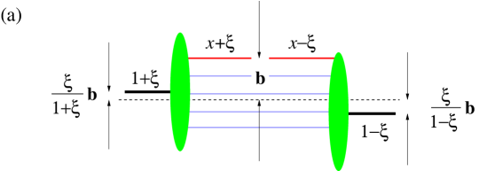
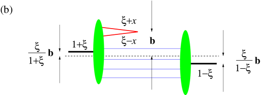
Figure 1: Representation of a GPD in impact parameter space. Plus-momentum fractions refer to the average proton momentum $\frac{1}{2}(p+p^{\prime})$ and are indicated above or below lines. The region $\xi\leq x\leq 1$ is shown in (a), and the region $|x|\leq\xi$ in (b).

Figure 1 shows the physical picture encoded in (18). GPDs in impact parameter space probe partons at transverse position ${\mathbf{b}}$, with the initial and final state proton localized around ${\mathbf{0}}$ but shifted relative to each other by an amount of order $\xi{\mathbf{b}}$. At the same time, the longitudinal momenta of the protons and hadrons are specified, in the same way as in the $t$-dependent GPDs. In the DGLAP regions $x\in[\xi,1]$ and $x\in[-1,-\xi]$, the impact parameter gives the location where a quark or antiquark is pulled out of and put back into the proton. In the ERBL region $x\in[-\xi,\xi]$ the impact parameter describes the transverse location of a quark-antiquark pair in the initial proton.

We remark that the shift of the transverse proton positions depends on $\xi$ but not on $x$. The information on the transverse location of partons in the proton is therefore not “washed out” when GPDs are integrated over $x$ with a weight depending on $x$ and $\xi$. As anticipated in [5] this implies that information is already contained in the scattering amplitudes of hard processes, where GPDs enter through just such a convolution in $x$. Notice also that for very small $\xi$ the difference between the proton positions becomes negligible compared to the impact parameter ${\mathbf{b}}$ of the struck quark. In this sense the situation is simpler for the impact parameter than for the longitudinal momentum fractions $x+\xi$ and $x-\xi$. Even at small $\xi$ their difference cannot be neglected when $x$ is of order $\xi$, which it typically is in the convolution with the hard scattering kernel of a physical process.

3 The overlap representation in ${\mathbf{b}}$-space

A physical interpretation of momentum space GPDs has been obtained in [6, 10] by writing them in terms of hadronic light-cone wave functions. We will now derive the analog of this in the mixed representation of definite plus-momentum and impact parameter.

3.1 Fock space and wave functions

A wave function representation of GPDs is naturally derived in the framework of light-cone quantization and in the gauge $A^{+}=0$. We will only recall essentials here; more detail can for instance be found in [6] or in [8]. In light-cone quantization the dynamically independent components of a quark field are given by the projection $q_{+}=\frac{1}{2}\gamma^{-}\gamma^{+}q$. At a given light-cone time, which we take as $z^{+}=0$, this can be expanded in terms of creation and annihilation operators for quarks and antiquarks of definite momentum,

$$q_{+}(0,z^{-},{\mathbf{z}}) = \int\frac{d^{2}{\mathbf{k}}\,dk^{+}}{16\pi^{3}k^{+}}\,\theta(k^{+})\,\sum_{\mu}\Big{[}\,b(k^{+},{\mathbf{k}},\mu)\,u_{+}(k^{+},\mu)\,e^{-ik^{+}z^{-}+i{\mathbf{k}}\cdot{\mathbf{z}}}$$ (20)

$$\hskip 83.00015pt{}+d^{\dagger}(k^{+},{\mathbf{k}},\mu)\,v_{+}(k^{+},\mu)\,e^{ik^{+}z^{-}-i{\mathbf{k}}\cdot{\mathbf{z}}}\,\Big{]},$$

where $\mu$ specifies the parton light-cone helicity. Operators for quarks and antiquarks with definite impact parameter are given by

$$\tilde{b}(k^{+},{\mathbf{b}},\mu) = \int\frac{d^{2}{\mathbf{k}}}{16\pi^{3}}\,b(k^{+},{\mathbf{k}},\mu)\,e^{i{\mathbf{k}}\cdot{\mathbf{b}}},$$

$$\tilde{d}(k^{+},{\mathbf{b}},\mu) = \int\frac{d^{2}{\mathbf{k}}}{16\pi^{3}}\,d(k^{+},{\mathbf{k}},\mu)\,e^{i{\mathbf{k}}\cdot{\mathbf{b}}}.$$ (21)

The good components of the quark field can then be rewritten as

$$q_{+}(0,z^{-},{\mathbf{b}}) = \int\frac{dk^{+}}{k^{+}}\,\theta(k^{+})\,\sum_{\mu}\Big{[}\,\tilde{b}(k^{+},{\mathbf{b}},\mu)\,u_{+}(k^{+},\mu)\,e^{-ik^{+}z^{-}}$$ (22)

$$\hskip 65.00009pt{}+\tilde{d}^{\dagger}(k^{+},{\mathbf{b}},\mu)\,v_{+}(k^{+},\mu)\,e^{ik^{+}z^{-}}\,\Big{]}.$$

Notice that for this to work it is essential that the good spinor components $u_{+}(k^{+},\mu)=\frac{1}{2}\gamma^{-}\gamma^{+}u(k,\mu)$ and $v_{+}(k^{+},\mu)=\frac{1}{2}\gamma^{-}\gamma^{+}v(k,\mu)$ are independent of ${\mathbf{k}}$. In other words, for the good field components one can specify the light-cone helicity of a parton without specifying its transverse momentum. In full analogy to (3.1) one can define annihilation operators $\tilde{a}(k^{+},{\mathbf{b}},\mu)$ for gluons with definite impact parameter from their momentum space counterparts $a(k^{+},{\mathbf{k}},\mu)$.

The Fock state expansion of a hadron state in momentum space reads

$$|p^{+},{\mathbf{p}},\lambda\rangle=\sum_{N,\beta}\,\frac{1}{\sqrt{f_{N\beta}}}\int\prod_{i=1}^{N}\,\frac{dx_{i}}{\sqrt{x_{i}}}\,\delta\Big{(}1-\sum_{i=1}^{N}x_{i}\Big{)}\;\frac{1}{(16\pi^{3})^{N-1}}\,\prod_{i=1}^{N}d^{2}{\mathbf{k}}_{i}\;\delta^{(2)}\Big{(}{\mathbf{p}}-\sum_{i=1}^{N}{\mathbf{k}}_{i}\Big{)}\;$$

$$\times \psi^{\lambda}_{N\beta}(x_{i},{\mathbf{k}}_{i}-x_{i}{\mathbf{p}})\,\prod_{i=1}^{N_{q}}\,b^{\dagger}(x_{i}p^{+},{\mathbf{k}}_{i})\prod_{i=N_{q}+1}^{N_{q}+N_{\bar{q}}}d^{\,{\dagger}}(x_{i}p^{+},{\mathbf{k}}_{i})\prod_{i=N_{q}+N_{\bar{q}}+1}^{N}a^{\dagger}(x_{i}p^{+},{\mathbf{k}}_{i})\,|\,0\rangle$$

using the conventions of [6]. $N$ specifies the number of partons in a Fock state, and $\beta$ collectively labels its parton composition and the discrete quantum numbers (flavor, color, helicity) for each parton. $f_{N\beta}$ is a normalization constant providing a factor $n!$ for each subset of $n$ partons with identical discrete quantum numbers; for ease of writing we have omitted labels for these quantum numbers in the creation operators. Notice that the wave functions depend on the momentum variables of each parton only via the light-cone momentum fraction $x^{\phantom{+}}_{i}=k_{i}^{+}/p^{+}$ and its transverse momentum ${\mathbf{k}}_{i}-x_{i}{\mathbf{p}}$ relative to the one of the hadron.

Using the inverse transforms of (3.1) it is easy to obtain from (3.1) the Fock state decomposition for a transversely localized proton state (12) in terms of transversely localized partons:

$$|p^{+},{\mathbf{b}},\lambda\rangle=\sum_{N,\beta}\,\frac{1}{\sqrt{f_{N\beta}}}\int\prod_{i=1}^{N}\,\frac{dx_{i}}{\sqrt{x_{i}}}\,\delta\Big{(}1-\sum_{i=1}^{N}x_{i}\Big{)}\;(4\pi)^{N-1}\,\prod_{i=1}^{N}d^{2}{\mathbf{b}}_{i}\;\delta^{(2)}\Big{(}{\mathbf{b}}-\sum_{i=1}^{N}x_{i}{\mathbf{b}}_{i}\Big{)}\;$$

$$\times \widetilde{\psi}^{\lambda}_{N\beta}(x_{i},{\mathbf{b}}_{i}-{\mathbf{b}})\,\prod_{i=1}^{N_{q}}\,\tilde{b}^{\dagger}(x_{i}p^{+},{\mathbf{b}}_{i})\prod_{i=N_{q}+1}^{N_{q}+N_{\bar{q}}}\tilde{d}^{\,{\dagger}}(x_{i}p^{+},{\mathbf{b}}_{i})\prod_{i=N_{q}+N_{\bar{q}}+1}^{N}\tilde{a}^{\dagger}(x_{i}p^{+},{\mathbf{b}}_{i})\,|\,0\rangle.$$

The wave functions for definite transverse momentum or impact parameter are related by

$$\widetilde{\psi}_{N\beta}^{\lambda}(x_{i},{\mathbf{b}}_{i}-{\mathbf{b}}) = \int[d^{2}{\mathbf{k}}]_{N}\,\exp\!\Big{[}i\sum_{i=1}^{N}{\mathbf{k}}_{i}\cdot{\mathbf{b}}_{i}\Big{]}\,\psi^{\lambda}_{N\beta}(x_{i},{\mathbf{k}}_{i})\hskip 30.00005pt\mbox{with~{}}{\mathbf{b}}=\sum_{i=1}^{N}x_{i}{\mathbf{b}}_{i}\,,$$

$$\psi_{N\beta}^{\lambda}(x_{i},{\mathbf{k}}_{i}-x_{i}{\mathbf{p}}) = \int[d^{2}{\mathbf{b}}]_{N}\,\exp\!\Big{[}{-i}\sum_{i=1}^{N}{\mathbf{k}}_{i}\cdot{\mathbf{b}}_{i}\Big{]}\,\widetilde{\psi}^{\lambda}_{N\beta}(x_{i},{\mathbf{b}}_{i})\hskip 18.00005pt\mbox{with~{}}{\mathbf{p}}=\sum_{i=1}^{N}{\mathbf{k}}_{i}\,,$$

and normalized to

$$P^{\lambda}_{N\beta}\;=\;\int[dx]_{N}\,[d^{2}{\mathbf{k}}_{N}]\;\Big{|}\psi^{\lambda}_{N\beta}(x_{i},{\mathbf{k}}_{i})\Big{|}^{2}\;=\;\int[dx]_{N}\,[d^{2}{\mathbf{b}}_{N}]\;\Big{|}\widetilde{\psi}^{\lambda}_{N\beta}(x_{i},{\mathbf{b}}_{i})\Big{|}^{2},$$ (26)

where $P^{\lambda}_{N\beta}$ is the probability to find the corresponding Fock state in the proton, so that in total $\sum_{N,\beta}P^{\lambda}_{N\beta}=1$. Here we have used the shorthand notation

$$[d^{2}{\mathbf{k}}]_{N} = \frac{1}{(16\pi^{3})^{N-1}}\prod_{i=1}^{N}d^{2}{\mathbf{k}}_{i}\;\delta^{(2)}\Big{(}\sum_{i=1}^{N}{\mathbf{k}}_{i}\Big{)},$$

$${}[d^{2}{\mathbf{b}}]_{N} = (4\pi)^{N-1}\prod_{i=1}^{N}d^{2}{\mathbf{b}}_{i}\;\delta^{(2)}\Big{(}\sum_{i=1}^{N}x_{i}{\mathbf{b}}_{i}\Big{)},$$

$${}[dx]_{N} = \prod_{i=1}^{N}dx_{i}\;\delta\Big{(}1-\sum_{i=1}^{N}x_{i}\Big{)}$$ (27)

for the $N$-parton integration elements.

Let us briefly discuss the Fock state decomposition in impact parameter form (3.1). The parton $i$ is transversely localized at ${\mathbf{b}}_{i}$, but due to translation invariance the wave function $\widetilde{\psi}_{N\beta}$ depends only on its position relative to the center ${\mathbf{b}}$ of the proton. The constraint

$${\mathbf{b}}=\sum_{i=1}^{N}x_{i}{\mathbf{b}}_{i}$$ (28)

identifies ${\mathbf{b}}$ as the “center of plus-momentum” [11] or “transverse center of momentum” [12] of the partons in each separate Fock state $(N\beta)$. This constraint is due to the invariance of the light-cone formulation under transverse boosts. Technically, it arises in the derivation of (3.1) from (3.1) because the wave functions for proton states with different transverse momenta ${\mathbf{p}}$ have the same functional form $\psi^{\lambda}_{N\beta}(x_{i},{\mathbf{k}}_{i}-x_{i}{\mathbf{p}})$. Notice the analogy of this situation with nonrelativistic mechanics [11, 12]. The transverse boosts (5) have the same form as a Galilean transformation in two dimensions, with $k^{+}$ corresponding to the mass $m$ of a particle , and ${\mathbf{v}}$ to the velocity characterizing the transformation. The conserved quantity corresponding to the transverse center of momentum (28) is the center of mass $\sum m_{i}{\mathbf{r}}_{i}/\sum m_{i}$ of an $N$-body system.

3.2 The wave function representation of GPDs

After the preparations of the preceding subsection it is easy to write the matrix elements ${\cal H}_{\lambda^{\prime}\lambda}$ and ${\cal I}_{\lambda^{\prime}\lambda}$ in terms of wave functions $\widetilde{\psi}^{\lambda}_{N\beta}$. This can be done either by transforming the known representation of ${\cal H}_{\lambda^{\prime}\lambda}$ in terms of $\psi^{\lambda}_{N\beta}$, or by repeating the derivation given in [6] directly in the impact parameter formulation. The result in the DGLAP region $x\in[\xi,1]$ is

$${\cal I}_{\lambda^{\prime}\lambda}(x,\xi,{\mathbf{b}})\;=\;\sum_{N,\beta}\sqrt{1-\xi^{2}}^{\,1-N}\,\sum_{j=q}\;\int[dx]_{N}\,[d^{2}{\mathbf{b}}]_{N}$$

$$\times \delta(x-x_{j})\;\delta^{(2)}\Big{(}{\mathbf{b}}-{\mathbf{b}}_{j}\Big{)}\;\widetilde{\psi}_{N\beta}^{*\,\lambda^{\prime}}(x_{i}^{\rm out},{\mathbf{b}}_{i}^{\phantom{t}}-{\mathbf{b}}_{0}^{\rm out})\,\widetilde{\psi}_{N\beta}^{\lambda}(x_{i}^{\rm in},{\mathbf{b}}_{i}^{\phantom{t}}-{\mathbf{b}}_{0}^{\rm in})\,$$

with wave function arguments

$$x_{i}^{\rm in} = \frac{x_{i}}{1+\xi},\hskip 37.00002ptx_{i}^{\rm out}\;=\;\frac{x_{i}}{1-\xi}\qquad\qquad\mbox{for~{}}i\neq j,$$

$$x_{j}^{\rm in} = \frac{x_{j}+\xi}{1+\xi},\hskip 35.00005ptx_{j}^{\rm out}=\;\frac{x_{j}-\xi}{1-\xi},$$ (30)

and transverse locations of the proton states

$${\mathbf{b}}_{0}^{\rm in} = \frac{\xi}{1+\xi}\,{\mathbf{b}}_{j},\qquad{\mathbf{b}}_{0}^{\rm out}\;=\;-\frac{\xi}{1-\xi}\,{\mathbf{b}}_{j}.\hskip 55.00008pt$$ (31)

The label $j$ denotes the struck parton and is summed over all quarks with appropriate flavor in a given Fock state, and the labels $(N,\beta)$ are summed over the corresponding Fock states. The representation in the DGLAP region $x\in[-1,-\xi]$ is obtained from (3.2) by reversing the overall sign, by changing $\delta(x-x_{j})$ into $\delta(x+x_{j})$, and by summing $j$ over antiquarks. In the ERBL region $x\in[-\xi,\xi]$ we have

$${\cal I}_{\lambda^{\prime}\lambda}(x,\xi,{\mathbf{b}})=\sum_{N,\beta,\beta^{\prime}}\sqrt{1-\xi}^{\,2-N}\sqrt{1+\xi}^{\,-N}\,\sum_{j,j^{\prime}}\frac{1}{\sqrt{\rule{0.0pt}{6.02773pt}n_{j}n_{j^{\prime}}}}\,$$

$$\times \int dx_{j}\prod_{i\neq j,j^{\prime}}dx_{i}\;\delta\Big{(}1-\xi-\sum_{i\neq j,j^{\prime}}x_{i}\Big{)}$$

$$\times (4\pi)^{N-1}\,\int d^{2}{\mathbf{b}}_{j}\prod_{i\neq j,j^{\prime}}d^{2}{\mathbf{b}}_{i}\;\delta^{(2)}\Big{(}\xi{\mathbf{b}}_{j}+\sum_{i\neq j,j^{\prime}}x_{i}{\mathbf{b}}_{i}\Big{)}$$

$$\times \delta(x-x_{j})\;\delta^{(2)}\Big{(}{\mathbf{b}}-{\mathbf{b}}_{j}\Big{)}\;\widetilde{\psi}_{N-1,\,\beta^{\prime}}^{*\,\lambda^{\prime}}(x_{i}^{\rm out},{\mathbf{b}}_{i}^{\phantom{t}}-{\mathbf{b}}_{0}^{\rm out})\,\widetilde{\psi}_{N+1,\,\beta}^{\lambda}(x_{i}^{\rm in},{\mathbf{b}}_{i}^{\phantom{t}}-{\mathbf{b}}_{0}^{\rm in})$$

with ${\mathbf{b}}_{0}^{\rm in}$ and ${\mathbf{b}}_{0}^{\rm out}$ as in (31) and

$$x_{i}^{\rm in} = \frac{x_{i}}{1+\xi},\qquad x_{i}^{\rm out}\;=\;\frac{x_{i}}{1-\xi}\qquad\mbox{for~{}}i\neq j,j^{\prime},$$

$$x_{j}^{\rm in} = \frac{\xi+x_{j}}{1+\xi},\qquad x_{j^{\prime}}^{\rm in}\;=\;\frac{\xi-x_{j}}{1+\xi}.$$ (33)

The partons $j,j^{\prime}$ are the ones emitted from the initial proton, and in (3.2) one has to sum over all quarks $j$ and antiquarks $j^{\prime}$ with opposite helicities, opposite color, and appropriate flavor in the initial state proton, over all Fock states $(N+1,\beta)$ containing such a $q\bar{q}$ pair, and over all Fock states $(N-1,\beta^{\prime})$ of the final state proton with matching quantum numbers for the spectator partons $i\neq j,j^{\prime}$. The statistical factors $n_{j}$ ($n_{j^{\prime}}$) give the number of (anti)quarks in the Fock state $(N+1,\beta)$ that have the same discrete quantum numbers as the (anti)quark pulled out of the target. The impact parameter representations for quark helicity dependent and for gluon GPDs are analogous to (3.2) and (3.2); the relevant modifications can easily be deduced from the momentum space expressions in [6].

If one defines the impact parameter GPDs with an additional Gaussian weight $G({\mathbf{D}},\,{\mathbf{D}}^{2}_{\sigma})$ as in (18) then one simply has to replace

$$\delta^{(2)}\Big{(}{\mathbf{b}}-{\mathbf{b}}_{j}\Big{)}\to\frac{{{\mathbf{D}}^{2}_{\sigma}}}{2\pi}\;G\!\left({\mathbf{b}}-{\mathbf{b}}_{j},\,\frac{1}{{\mathbf{D}}^{2}_{\sigma}}\right)$$ (34)

in (3.2) and (3.2). This shows again that with data for ${\mathbf{D}}^{2}$ up to order ${\mathbf{D}}^{2}_{\sigma}$ one can obtain information in impact parameter space to an accuracy of order $1/|{\mathbf{D}}_{\sigma}|$. We remark that the precise implementation of this is different in our result (18), where the transverse location of each proton is smeared out independently, and in (34), where the smearing is over the location of the struck parton or parton pair, with a smearing of the proton positions induced by (31).

The physical interpretation of the overlap formulae (3.2) and (3.2) is the same as the one we have obtained in section 2.3 and illustrated in Fig. 1. We now see why for $\xi\neq 0$ the transverse location of the proton is different before and after the scattering: according to our discussion in subsection 3.1, its transverse center of momentum is shifted because the proton is subject to a finite transfer of plus-momentum. We thus find that GPDs at nonzero $\xi$ correlate hadronic wave functions with both different plus-momentum fractions and different transverse positions of the partons. Notice however that the difference in transverse positions is a global shift in each wave function; the relative transverse distances between the partons in a hadron are the same before and after the scattering.

3.3 Positivity constraints

Positivity constraints for GPDs in the impact parameter representation have recently been considered by Pobylitsa in a very general framework [13]. We shall not elaborate on this subject in detail, but only give a set of inequalities that readily follow from the overlap representation (3.2) for ${\cal I}_{\lambda^{\prime}\lambda}$ in the DGLAP region. This representation has the structure of a scalar product $(\phi_{-\xi}^{\,\lambda^{\prime}}\,|\,\phi_{\xi}^{\lambda})$ in the Hilbert space of wave functions, with

$$\phi_{\xi}^{\lambda}(x_{i},{\mathbf{b}}_{i};N,\beta) = \sqrt{1+\xi}^{\,1-N}\,\widetilde{\psi}^{\lambda}_{N\beta}(x_{i}^{\rm in},{\mathbf{b}}_{i}-{\mathbf{b}}_{0}^{\rm in}),$$

$$\phi_{-\xi}^{\,\lambda^{\prime}}(x_{i},{\mathbf{b}}_{i};N,\beta) = \sqrt{1-\xi}^{\,1-N}\,\widetilde{\psi}^{\lambda^{\prime}}_{N\beta}(x_{i}^{\rm out},{\mathbf{b}}_{i}-{\mathbf{b}}_{0}^{\rm out}).$$ (35)

For $\xi=0$ this implies that ${\cal I}_{++}(x,0,{\mathbf{b}})$ must be real and positive if $x\geq 0$ and negative if $x\leq 0$, as observed in [14]. Furthermore we have the Schwartz inequality $|(\phi_{-\xi}^{\,\lambda^{\prime}}\,|\,\phi_{\xi}^{\lambda})|^{2}\leq(\phi_{-\xi}^{\,\lambda^{\prime}}\,|\,\phi_{-\xi}^{\,\lambda^{\prime}})\,(\phi_{\xi}^{\lambda}\,|\,\phi_{\xi}^{\lambda})$, which after suitable changes of integration variables in (3.2) gives

$$(1-\xi^{2})^{5}\,\Big{|}\,{\cal I}_{\lambda^{\prime}\lambda}(x,\xi,{\mathbf{b}})\,\Big{|}^{2}\leq{\cal I}_{++}\Big{(}\frac{x-\xi}{1-\xi},0,\frac{{\mathbf{b}}}{1-\xi}\Big{)}\;{\cal I}_{++}\Big{(}\frac{x+\xi}{1+\xi},0,\frac{{\mathbf{b}}}{1+\xi}\Big{)}$$ (36)

for $\xi\leq x\leq 1$ and any combination $\lambda^{\prime},\lambda$ of proton helicities. Further relations are obtained by replacing ${\cal I}$ with the combinations ${\cal I}\pm\widetilde{\cal I}$ for definite parton helicity. More detailed inequalities involving the various proton and parton helicity combinations can be obtained using the matrix structure in the helicities, as shown in [15].

4 Special cases

The wave function representation makes explicit in which way GPDs probe the longitudinal and transverse structure of a hadron in a correlated way. In particular we have seen that for finite $\xi$ they are correlations of wave functions where the partons differ both in longitudinal momentum and in impact parameter by an amount controlled by $\xi$. In this section we briefly discuss the type of information one obtains in some well-known special cases.

4.1 The limit $\xi=0$

In the case $\xi=0$ (where ${\mathbf{D}}$ coincides with the transverse momentum transfer ${\mathbf{p}}^{\prime}-{\mathbf{p}}$) the wave function representation (3.2) becomes particularly simple, with

$${\cal I}_{\lambda^{\prime}\lambda}(x,0,{\mathbf{b}})\,=\,\sum_{N,\beta}\sum_{j=q}\,\int[dx]_{N}\,[d^{2}{\mathbf{b}}]_{N}\,$$

$$\times \delta(x-x_{j})\;\delta^{(2)}\Big{(}{\mathbf{b}}-{\mathbf{b}}_{j}\Big{)}\;\widetilde{\psi}_{N\beta}^{*\,\lambda^{\prime}}(x_{i},{\mathbf{b}}_{i})\,\widetilde{\psi}_{N\beta}^{\lambda}(x_{i},{\mathbf{b}}_{i}).$$

for $x\geq 0$ and an analogous relation for $x\leq 0$. We see that if in addition one takes the same spin state for the two proton states, the Fourier transform of $H(x,0,t)$ is expressed through squared wave functions and thus has a density interpretation. For the Fourier transform of $\tilde{H}(x,0,t)$ one obtains the difference of squared wave functions for a right-handed and a left-handed struck quark or antiquark. At $\xi=0$ the distribution $E$ only appears in the matrix element for proton helicity flip, and its Fourier transform in ${\cal I}_{-+}(x,0,{\mathbf{b}})$ correlates wave functions with identical parton configurations but with opposite helicities of the parent proton. Giving it a probability interpretation is more involved [14], and we will not elaborate on this issue. Notice finally that no information is obtained about $\tilde{E}$ by setting $\xi=0$ in the appropriate matrix elements, where due to its definition (2.1) it is accompanied by at least one factor of $\xi$.

Inverting the Fourier transform (8) we see that the usual quark density $q(x)=H(x,0,0)$ can be written as the integral of ${\cal I}_{++}(x,0,{\mathbf{b}})$ over ${\mathbf{b}}$, which removes the $\delta^{(2)}({\mathbf{b}}-{\mathbf{b}}_{j})$ on the right-hand side of (4.1). This makes it explicit that ordinary parton densities specify the longitudinal momentum fraction of the struck parton, averaged over its transverse position in the target.

4.2 Form factors

Integrating $H$, $E$, $\tilde{H}$, $\tilde{E}$ over $x$ one obtains the elastic form factors of the quark vector and axial vector current. Since the form factors are independent of $\xi$ one can evaluate their wave function representation in a frame with $\xi=0$, which was the original choice of Drell and Yan [16]. Introducing Dirac and Pauli form factors for each separate quark flavor,

$$\langle p^{\prime},\lambda^{\prime}|\,\bar{q}(0)\gamma^{\mu}q(0)\,|p,\lambda\rangle=\bar{u}(p^{\prime},\lambda^{\prime})\left[\,F_{1}^{q}(t)\,{\gamma}^{\mu}+F_{2}^{q}(t)\,\frac{i{\sigma}^{\mu\alpha}(p^{\prime}-p)_{\alpha}}{2m}\,\right]u(p,\lambda),$$ (38)

we have impact parameter representations

$$\frac{1}{4\pi}\int_{-\infty}^{0}\!dt\,J_{0}\Big{(}|{\mathbf{b}}|\sqrt{-t}\Big{)}\,F_{1}^{q}(t)$$

$$= \sum_{N,\beta}\,\sum_{j=q,\bar{q}}\sigma_{j}\,\int[dx]_{N}\,[d^{2}{\mathbf{b}}]_{N}\;\delta^{(2)}\Big{(}{\mathbf{b}}-{\mathbf{b}}_{j}\Big{)}\;\Big{|}\widetilde{\psi}_{N\beta}^{\lambda}(x_{i},{\mathbf{b}}_{i})\Big{|}^{2},$$

$$\frac{1}{4\pi}\,\frac{b^{2}-ib^{1}}{|{\mathbf{b}}|}\int_{-\infty}^{0}dt\,J_{1}\Big{(}|{\mathbf{b}}|\sqrt{-t}\Big{)}\;\frac{\sqrt{-t}}{2m}\,F_{2}^{q}(t)$$

$$= \sum_{N,\beta}\,\sum_{j=q,\bar{q}}\sigma_{j}\,\int[dx]_{N}\,[d^{2}{\mathbf{b}}]_{N}\;\delta^{(2)}\Big{(}{\mathbf{b}}-{\mathbf{b}}_{j}\Big{)}\;\widetilde{\psi}_{N\beta}^{*\lambda^{\prime}}(x_{i},{\mathbf{b}}_{i})\,\widetilde{\psi}_{N\beta}^{\lambda}(x_{i},{\mathbf{b}}_{i}),$$

where $\sigma_{j}$ is $+1$ for quarks and $-1$ for antiquarks, and $\lambda=+{\textstyle\frac{1}{2}}$, $\lambda^{\prime}=-{\textstyle\frac{1}{2}}$. A corresponding relation exists for the Fourier transform of the axial form factor. The pseudoscalar form factor decouples at $\xi=0$ and like $\tilde{E}$ requires evaluation in a frame with nonzero $\xi$. We see that the Fourier transform of the Dirac form factor $F_{1}^{q}$ has an immediate density interpretation, whereas the Pauli form factor $F_{2}^{q}$ correlates wave functions for opposite proton helicities. To be precise, the Fourier transforms in (4.2) describe the transverse location of partons in a fast moving proton, irrespective of their longitudinal momenta [11]. This is the opposite of what we had for the usual parton densities, which contain purely longitudinal information. The interpretation of an elastic form factor in a frame where the proton moves fast may seem unusual, but note that we are describing hadron structure in terms of quarks, antiquarks, and gluons here, so that such a frame is in fact very adequate.

Taking higher moments in $x$ gives form factors of operators containing derivatives. In this case, information on longitudinal structure is retained in the form of a momentum dependent weight. The simplest example is the quark part of the energy momentum tensor, whose $(++)$ component can be written as [2]

$$\langle p^{\prime},\lambda^{\prime}|\,T_{q}^{++}(0)\,|p,\lambda\rangle = \bar{u}(p^{\prime},\lambda^{\prime})\left[\,A^{q}(t)\,P^{+}\gamma^{+}+B^{q}(t)\,\frac{P^{+}i{\sigma}^{+\alpha}(p^{\prime}-p)_{\alpha}}{2m}\right.$$ (40)

$$\hskip 28.99997pt\left.{}+C^{q}(t)\,\frac{(p^{\prime}-p)^{+}(p^{\prime}-p)^{+}}{m}\,\right]u(p,\lambda)$$

and is related with $\int dx\,xH$ and $\int dx\,xE$ by a sum rule. In a frame with $\xi=0$ the form factor $C^{q}$ decouples and one is left with $A^{q}$ and $B^{q}$. Their representation in terms of momentum space wave functions has been discussed in [17]. In impact parameter space it is obtained from (4.2) by replacing $F_{1}^{q}$ with $A^{q}_{\phantom{1}}$ and $F_{2}^{q}$ with $B^{q}_{\phantom{1}}$ on the left, and $\sigma_{j}$ with $x_{j}$ on the right. In other words, the contributions from quarks and antiquarks $j$ now come with the same sign and weighted by their momentum fractions. In particular, the Fourier transform of $A^{q}$ describes the transverse distribution of the longitudinal momentum carried by quarks and antiquarks of a given flavor. Integrating it over ${\mathbf{b}}$ one obtains the second moment $\int dx\,x(q+\bar{q})$ of quark and antiquark distributions.

5 A tale of two scales

So far we have suppressed the dependence of GPDs on the factorization scale $\mu$, which in a physical process is provided by the hard scale $Q$. The dependence on this scale is given by well-known evolution equations [1, 2, 3, 18] of the general form

$$\mu\,\frac{\partial}{\partial\mu}H(x,\xi,t;\mu)=\int dy\;K(x,y,\xi;\alpha_{s}(\mu))\,H(y,\xi,t;\mu),$$ (41)

with evolution kernels $K$ known up to two-loop accuracy [19]. Important for us is that these equations involve GPDs at the same $t$ and $\xi$, so that taking the Fourier transform with respect to ${\mathbf{D}}$ does not alter their structure. The evolution equations for GPDs in impact parameter space are hence the same as for their $t$-dependent counterparts.

The physical meaning of $\mu$ in our context is essentially as in the case of ordinary parton distributions. We recall that because of the short-distance singularities of QCD, light-cone wave functions and the underlying Fock state decomposition must be renormalized [8]. For our purpose it is useful to understand the associated renormalization scale $\mu$ as a cutoff on transverse momenta [20]. Quarks and gluons in the presence of this cutoff are then “elementary” down to a transverse resolution of order $\mu^{-1}$—loosely speaking they have a transverse extension of that size. The wave functions in our overlap representations refer to partons at a given scale $\mu$. An impact parameter GPD in the DGLAP region may thus be interpreted as describing the longitudinal momentum and transverse location of a quark with transverse size $\mu^{-1}$. At larger values of $\mu$, this quark may be seen as consisting of a quark plus a gluon, i.e., one will start to resolve its “substructure”. In the ERBL region a GPD in impact parameter space describes a $q\bar{q}$-pair, where quark and antiquark are each of size $\mu^{-1}$ and at the same transverse position in the proton, to an accuracy again of order $\mu^{-1}$.

The role played by $\mu^{-1}$ is to be contrasted with the transverse resolution $\sigma\sim(|t|_{\rm max}-|t|_{\rm min})^{-1/2}$ discussed in sections 2.3 and 3.2, which refers to the transverse location of a parton within its parent hadron. In other words, the momentum transfer $t$ is related to where a parton is found in the proton, whereas $\mu^{2}$ determines what is meant by “a parton”. An ordinary quark distribution at very large $\mu^{2}$, for instance, contains information on the longitudinal momenta of quarks seen with very fine transverse resolution, but no information at all on where quarks are located in the transverse plane. To use an analog from optics consider a cell under a microscope. Then $\mu^{-1}$ corresponds to the optical resolution and limits which details of the cell one can see. The analog of $(|t|_{\rm max}-|t|_{\rm min})^{-1/2}$ specifies how precisely one controls the position of the cell under the objective, in order to determine where the magnified detail is located within the cell.

At this point we can make a comment on the representation (4.2) of the elastic form factors $F_{1}(t)$ and $F_{2}(t)$ in terms of wave functions for quarks, antiquarks and gluons. At small values of $-t$, say below 1 GeV², one may wonder how such a description is possible, given that the form factors are measured in elastic scattering processes whose momentum transfer $t$ is insufficient to resolve any partonic structure at all. The solution of this apparent paradox is that these form factors are independent of a renormalization scale $\mu^{2}$ because the quark vector current $\bar{q}(z)\gamma^{\mu}q(z)$ is conserved. They are hence the same when evaluated at $\mu^{2}\sim-t$ or at $\mu^{2}$ of several GeV². Physically speaking, the transverse distribution of charge in the proton is independent of how much substructure is resolved, so that one may represent this charge distribution as due to quarks and antiquarks, even though one has not resolved them explicitly. In this sense, $F_{1}(t)$ and $F_{2}(t)$ at small $t$ do contain information on partons, but this information is not specific to these degrees of freedom.

Notice that the situation is different for form factors of other operators, which are given by higher moments of GPDs in $x$. The quark energy-momentum tensor for instance does depend on the renormalization scale, and the information of its form factors is specific to the value of $\mu$. As $\mu$ increases, the average momentum carried by quarks at a given impact parameter will become smaller, since one resolves processes where the quarks lose momentum by radiating gluons. In the case of energy-momentum one still has a conserved current when summing over all quark flavors and gluons, but this does not hold for other local operators connected to moments of GPDs.

6 Unintegrated parton distributions

Apart from GPDs, there is another class of nonperturbative functions that carry information not only on longitudinal but also on transverse hadron structure. These are $k_{T}$-dependent or unintegrated parton distributions. Let us see how the information they contain looks like when expressed in terms of transverse position, and contrast it with the picture we have obtained for GPDs. For simplicity we will restrict ourselves to forward distributions and set $p=p^{\prime}$. It is then sufficient to consider a frame with ${\mathbf{p}}=0$. Following the naming scheme of [21] we define

$$f_{1}(x,{\mathbf{k}})=\int\frac{d^{2}{\mathbf{z}}\,dz^{-}}{16\pi^{3}}\;e^{ixp^{+}z^{-}-i{\mathbf{k}}\cdot{\mathbf{z}}}\;\langle p,\lambda|\,\bar{q}(0,-{\textstyle\frac{1}{2}}z^{-},-{\textstyle\frac{1}{2}}{\mathbf{z}})\,\gamma^{+}q(0,{\textstyle\frac{1}{2}}z^{-},{\textstyle\frac{1}{2}}{\mathbf{z}})\,|p,\lambda\rangle,$$ (42)

which is related to the usual quark density by $\int d^{2}{\mathbf{k}}\,f_{1}(x,{\mathbf{k}})=q(x)$. We suppress again the dependence on the factorization scale $\mu$, whose discussion proceeds in analogy with the preceding section. A word of warning is in order concerning the absence of the usual Wilson line between the operators $\bar{q}$ and $q$. These are now taken at different transverse positions $\pm{\textstyle\frac{1}{2}}{\mathbf{z}}$, so that a Wilson line appears even in the gauge $A^{+}=0$, except for particular choices of the integration path. As recently discussed in [22] there is subtle physics encoded in the choice of path and the Wilson line. This is beyond the purpose of our present investigation, which is a basic understanding of the spacial information contained in various types of parton distributions. The same holds for recent work where it was argued that even for the usual parton distributions, with ${\mathbf{z}}=0$, physical effects of the Wilson line are not correctly reproduced in light-cone gauge [23].

In transverse momentum space, the distribution $f_{1}(x,{\mathbf{k}})$ can be interpreted as a probability density. This is readily seen from its wave function representation, which involves $|\psi(x_{i},{\mathbf{k}}_{i})|^{2}$, with the wave function arguments of the struck parton fixed to be $x_{j}=x$ and ${\mathbf{k}}_{j}={\mathbf{k}}$. In terms of impact parameter wave functions we have

$$\int d^{2}{\mathbf{k}}\;e^{i{\mathbf{k}}\cdot{\mathbf{z}}}\,f_{1}(x,{\mathbf{k}})=\sum_{N,\beta}\,\sum_{j=q}\,\int[dx]_{N}\,[d^{2}{\mathbf{b}}]_{N}$$

$$\times \delta(x-x_{j})\;\widetilde{\psi}_{N\beta}^{*\,\lambda}(x_{i},{\mathbf{b}}^{\rm out}_{i}-{\mathbf{b}}_{0}^{\rm out})\,\widetilde{\psi}_{N\beta}^{\lambda}(x_{i},{\mathbf{b}}^{\rm in}_{i}-{\mathbf{b}}_{0}^{\rm in})\,$$

for $x>0$, with wave function arguments

$${\mathbf{b}}_{i}^{\rm in} = {\mathbf{b}}_{i}^{\rm out}\;=\;{\mathbf{b}}_{i}\hskip 35.00005pt\mbox{~{}for~{}}i\neq j,$$

$${\mathbf{b}}_{j}^{\rm in} = {\mathbf{b}}_{j}+\frac{{\mathbf{z}}}{2},\qquad{\mathbf{b}}_{j}^{\rm out}\;=\;{\mathbf{b}}_{j}-\frac{{\mathbf{z}}}{2},$$ (44)

and proton states centered at

$${\mathbf{b}}_{0}^{\rm in} = x\,\frac{{\mathbf{z}}}{2},\qquad\qquad{\mathbf{b}}_{0}^{\rm out}\;=\;{}-x\,\frac{{\mathbf{z}}}{2}.$$ (45)

The corresponding physical picture is represented in Fig. 2. As is already evident from the operator defining $f_{1}(x,{\mathbf{k}})$ in (42), we see that the struck quark is at a relative transverse distance ${\mathbf{z}}$ in the initial and the final state. Unintegrated parton distributions thus describe the correlation in transverse position of a single parton. Notice that, in contrast to the situation for GPDs, the struck quark now has a different transverse location relative to the spectator partons in the initial and the final state wave functions, in addition to the overall shift of the proton center of momentum dictated again by Lorentz invariance. The dependence of the Fourier transform (6) on ${\mathbf{z}}$ thus describes how much the transverse location of a single parton can vary in the proton wave function when all other partons are kept fixed. Notice finally that since $f_{1}(x,{\mathbf{k}})$ is measured at $t=0$, the overall position of the struck quark with respect to the center of the proton is integrated over in (6).

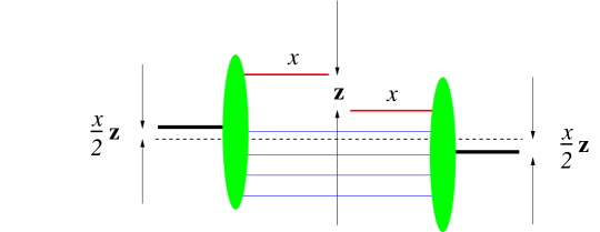
Figure 2: Impact parameter representation of an unintegrated parton distribution. ${\mathbf{z}}$ is the Fourier conjugate variable to the transverse momentum ${\mathbf{k}}$ of the struck parton.

The quantities that contain this information in addition are of course $k_{T}$ unintegrated GPDs. They have been used in an estimate of power corrections for hard exclusive processes in [24] and recently been discussed in the context of small-$x$ physics in [25]. Their impact parameter representation combines the characteristic features of (3.2) and (3.2) with those of (6). In the DGLAP region, both the average transverse position ${\mathbf{b}}$ and the relative offset ${\mathbf{z}}$ of the struck parton in the initial and final state are now specified, whereas the ERBL region describes a $q\bar{q}$-pair in the initial state proton, with an average transverse position ${\mathbf{b}}$ and a relative separation ${\mathbf{z}}$ between quark and antiquark.

7 Conclusions

A natural setting to represent the structure of a hadron in terms of quarks and gluons is a frame where the hadron moves fast. Its direction of motion and the two perpendicular ones then acquire different physical roles, and a comprehensive description of the hadron requires information both on the longitudinal and the transverse degrees of freedom. Generalized parton distributions are among the quantities that allow one to address such questions as: “How broad is the spatial transverse distribution of fast quarks compared with slow ones, and how does it compare with the spatial transverse distribution of gluons?”

Whereas the description of scattering processes is in momentum space, useful physical insight can be obtained in the mixed representation of longitudinal momentum and transverse position, or impact parameter. This representation is natural in various contexts, for instance in the description of high-energy scattering processes, see e.g. [26], or the resummation of Sudakov logarithms in hard reactions [27]. Burkardt has pointed out that for zero skewness $\xi$, GPDs in impact parameter space have the simple representation of a joint density in the longitudinal momentum of a parton and its transverse distribution in the proton, at least for helicity conserving transitions [4]. We find that the situation for nonzero $\xi$ is similar up to an important difference: as the proton loses longitudinal momentum its transverse position is shifted by an amount proportional to $\xi$. This is because as a consequence of Lorentz invariance the “transverse position” of the proton is the vector sum of the transverse positions of its partons weighted by their longitudinal momentum fractions. A more detailed picture is obtained by expressing GPDs in terms of impact parameter wave functions, related to the ones in momentum space by a Fourier transform. In addition to their longitudinal momentum fractions, the transverse distance of partons from the proton center differs in the initial and final state, but their relative distance to each other in a hadron stays the same. This is in contrast to the case of $k_{T}$-dependent (but forward) parton distributions, which in impact parameter space are correlation functions for the transverse distance of a single parton with respect to all other partons in the wave function.

All together, GPDs at nonzero $\xi$ describe quantum mechanical correlations within a hadron rather than probability densities, both in the transverse momentum and the impact parameter representations. Despite their complexity in detail, the underlying physical picture is simple, as shown in Fig. 1. As to achievable spatial resolution, GPDs measured in a process with hard scale $Q^{2}$ provides information on partons as seen with resolution $Q^{-1}$, whereas the invariant momentum transfer $|t|$ to the proton must be known from its minimum value $|t|_{\rm min}$ up to $|t|_{\rm max}$ in order to locate partons in the transverse plane to an accuracy of order $(|t|_{\rm max}-|t|_{\rm min})^{-1/2}$.

The kinematical factor in the positivity bound (36) is incorrect. The bound correctly reads

$$(1-\xi^{2})^{3}\,\Big{|}\,{\cal I}_{\lambda^{\prime}\lambda}(x,\xi,{\mathbf{b}})\,\Big{|}^{2}\leq{\cal I}_{++}\Big{(}\frac{x-\xi}{1-\xi},0,\frac{{\mathbf{b}}}{1-\xi}\Big{)}\;{\cal I}_{++}\Big{(}\frac{x+\xi}{1+\xi},0,\frac{{\mathbf{b}}}{1+\xi}\Big{)}.$$

Our corrected result agrees with inequality (25) in [13], taking into account the different normalization conventions here and there.

References

• [1] D. Müller, D. Robaschik, B. Geyer, F. M. Dittes, and J. Hořejši, Fortschr. Phys. 42, 101 (1994), hep-ph/9812448.
• [2] X.-D. Ji, Phys. Rev. Lett. 78, 610 (1997), hep-ph/9603249.
• [3] A. V. Radyushkin, Phys. Rev. D56, 5524 (1997), hep-ph/9704207.
• [4] M. Burkardt, Phys. Rev. D62, 071503 (2000), hep-ph/0005108.
• [5] J. P. Ralston and B. Pire, Phys. Rev. D66, 111501 (2002), hep-ph/0110075.
• [6] M. Diehl, T. Feldmann, R. Jakob, and P. Kroll, Nucl. Phys. B596, 33 (2001), Erratum-ibid. B605, 647 (2001), hep-ph/0009255.
• [7] J. B. Kogut and D. E. Soper, Phys. Rev. D1, 2901 (1970).
• [8] S. J. Brodsky and G. P. Lepage, in: A. H. Mueller (Ed.), Perturbative Quantum Chromodynamics, World Scientific, Singapore, 1989.
• [9] M. Diehl, Eur. Phys. J. C19, 485 (2001), hep-ph/0101335.
• [10] S. J. Brodsky, M. Diehl, and D. S. Hwang, Nucl. Phys. B596, 99 (2001), hep-ph/0009254.
• [11] D. E. Soper, Phys. Rev. D15, 1141 (1977).
• [12] M. Burkardt, hep-ph/0008051.
• [13] P. V. Pobylitsa, Phys. Rev. D66, 094002 (2002), hep-ph/0204337.
• [14] M. Burkardt, hep-ph/0105324.
• [15] P. V. Pobylitsa, Phys. Rev. D65, 077504 (2002), hep-ph/0112322;
P. V. Pobylitsa,
Phys. Rev. D65, 114015 (2002), hep-ph/0201030.
• [16] S. D. Drell and T.-M. Yan, Phys. Rev. Lett. 24, 181 (1970).
• [17] S. J. Brodsky, D. S. Hwang, B.-Q. Ma, and I. Schmidt, Nucl. Phys. B593, 311 (2001), hep-th/0003082.
• [18] J. Blümlein, B. Geyer, and D. Robaschik, Phys. Lett. B406, 161 (1997), hep-ph/9705264.
• [19] A. V. Belitsky, A. Freund, and D. Müller, Nucl. Phys. B574, 347 (2000), hep-ph/9912379.
• [20] J. B. Kogut and L. Susskind, Phys. Rev. D9, 3391 (1974).
• [21] P. J. Mulders and R. D. Tangerman, Nucl. Phys. B461, 197 (1996), hep-ph/9510301;
P. J. Mulders,
hep-ph/9912493.
• [22] J. C. Collins, Phys. Lett. B536, 43 (2002), hep-ph/0204004.
• [23] S. J. Brodsky, P. Hoyer, N. Marchal, S. Peigné, and F. Sannino, Phys. Rev. D65, 114025 (2002), hep-ph/0104291.
• [24] M. Vanderhaeghen, P. A. M. Guichon, and M. Guidal, Phys. Rev. D60, 094017 (1999), hep-ph/9905372.
• [25] A. D. Martin and M. G. Ryskin, Phys. Rev. D64, 094017 (2001), hep-ph/0107149.
• [26] O. Nachtmann, hep-ph/9609365;
M. Wüsthoff and A. D. Martin,
J. Phys. G25, R309 (1999), hep-ph/9909362.
• [27] J. C. Collins and D. E. Soper, Nucl. Phys. B193, 381 (1981), Erratum-ibid. B213, 545 (1983).
Erratum
Generalized parton distributions in impact parameter space
Eur. Phys. J. C25, 223 (2002), hep-ph/0205208
M. Diehl