Chapter 1 Lattice QCD

Christine Davies
University of Glasgow, UK

1 Introduction

Lattice QCD was invented, way ahead of its time, in 1974. It really became a useful technique in the 1990s when a huge amount of progress was made in the understanding and reduction of systematic errors. Now, we are poised to start a second lattice revolution with the onset of Teraflop supercomputing around the world and further improvements in methodology. This will enable calculations using lattice QCD to reach errors of a few percent, over the next five years. At this level, lattice results, where they exist, will be the theoretical calculations of choice for the experimental community.

It seems, then, a good time to review the fundamentals of lattice QCD, for an audience of experimental particle physicists. As ‘consumers’ of lattice calculations, it is important to be aware of how these calculations are done so that a critical assessment of different results can be made. I have tried to keep technical details to a minimum in what follows but it is necessary to understand some of them, to appreciate the significance and the limitations of the lattice results that you might want to use. For a more detailed discussion see, for example (Gupta, 1998) or (Di Pierro, 2001). This school is largely concerned with CP violation and heavy quark physics, so in Section 4 I concentrate on lattice results relevant to these areas.

2 Lattice QCD formalism and methods

2.1 The path integral approach

Lattice QCD is just QCD, no more and no less. We take the theory, express it in Feynman Path Integral language, and calculate the integral as well as we can. We would like to be able to do this in the continuous space-time of the real world, but this is not possible. Instead, we must break space-time up into a 4-d grid of points, i.e. a lattice (Figure 1), and evaluate the Feynman Path Integral by Monte Carlo methods on a computer. It turns out to be a calculation that requires a huge amount of computing power and tests the fastest supercomputers that we have.

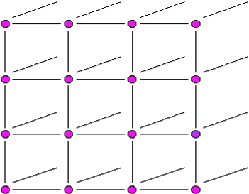
Figure 1: A 2-dimensional rendition of a 3-dimensional cubic lattice. Lattice QCD calculations use a 4-dimensional grid.

In the Feynman Path Integral approach, we first express the quantity that we want to calculate as the matrix element in the vacuum of an operator, $\bm{\mathcal{O}}$, which will be a product of quark and gluon fields so that, for example, $\bm{\mathcal{O}}=(\overline{\psi}\psi)_{y}(\overline{\psi}\psi)_{x}$. creates a hadron at a point $x$ and destroys it at a point $y$. We will discuss later other forms that $\bm{\mathcal{O}}$ might take to calculate useful quantities. Then:

$$\langle 0|\bm{\mathcal{O}}|0\rangle=\frac{{\displaystyle\int{[d\psi]\,[d\bar{\psi}]\,[dA_{\mu}]\,\bm{\mathcal{O}}[\psi,\overline{\psi},A]e^{-S}}}}{{\displaystyle\int{[d\psi]\,[d\bar{\psi}]\,[dA_{\mu}]e^{-S}}}}$$ (1)

where $S$ is the action, the integral of the Lagrangian:

$$S=\int\!{{\cal{L}}\,d^{4}x}.$$ (2)

We are using Euclidean space here (imaginary time) so that the integrand doesn’t contain the oscillatory $e^{iS}$, but the more easily integrated $e^{-S}$. The integral of Equation 1 can then be evaluated numerically if we can convert it to a finite-dimensional problem.

Currently the integral runs over all values of the quark and gluon fields $\psi$ and $A$ at every point in space-time. We need to make the number of space-time points (and therefore field variables) finite and we do this by taking a 4-d box of space-time and discretising it into a cubic grid, or lattice. It is then a relatively simple matter to transcribe the continuous theory onto the lattice, and we use the standard methods used for discretising e.g. differential equations for numerical solution. Continuous space-time $(x,t)$ becomes a grid of labelled points, $(x_{i},t_{i})$ or $(n_{i}a,n_{t}a)$ where $a$ is the spacing between the points, called the lattice spacing. The fields are then associated only with the sites, $\psi(x,t)\rightarrow\psi(n_{i},n_{t})$. The action must also be discretised, but this is also straightforward. The Lagrangian typically contains fields and derivatives of fields. The fields are replaced with fields at the lattice sites and the derivatives replaced with finite differences of these fields. The integral over space-time of the Lagrangian becomes a sum over all lattice sites: ($\int{d^{4}x}\rightarrow\sum_{n}a^{4}$). There are inevitably discretisation errors associated with this procedure (just as there are for differential equations) because the lattice Lagrangian only matches the continuum Lagrangian at $a$ = 0. At non-zero $a$ there are effectively additional unwanted terms in the lattice Lagrangian that are proportional to powers of $a$. We will discuss this further later. Another view of the lattice is that it provides an ultra-violet cut-off on the theory in momentum space, since no momenta larger than $\pi/a$ make sense (the wavelength is then smaller than $a$). In this way it is an alternative regularisation of QCD.

As an illustration of the simplicity of the discretisation procedure, let us consider a scalar field theory with Lagrangian

$${\cal{L}}=\frac{1}{2}(\partial_{\mu}\phi)^{2}+\frac{1}{2}m^{2}\phi^{2}+\lambda\phi^{4}.$$ (3)

The lattice action, $S$ is then

$$S=\sum_{n}a^{4}\left(\frac{1}{2}\sum_{\mu=1}^{4}\left[\frac{\phi(n+1_{\mu})-\phi(n-1_{\mu})}{2a}\right]^{2}+\frac{1}{2}m^{2}\phi^{2}(n)+\lambda\phi^{4}(n)\right).$$ (4)

The point $n+1_{\mu}$ is one lattice point up from the point $n$ in the $\mu$ direction. We are always free to rescale parameters and fields and we do this on the lattice, rescaling by powers of the lattice spacing, so that the parameters and fields we work with are dimensionless. Everything is then said to be in ‘lattice units’. In the scalar theory above we rescale to primed quantities where $\phi^{\prime}=\phi a,\;m^{\prime}=ma,\;\lambda^{\prime}=\lambda$. Then

$$S=\sum_{n}\left({\phi^{\prime}}^{2}(n)\left[2+\frac{1}{2}{m^{\prime}}^{2}\right]+\lambda^{\prime}{\phi^{\prime}}^{4}-\frac{1}{4}\sum_{\mu}\phi^{\prime}(n+1_{\mu})\phi^{\prime}(n-1_{\mu})\right).$$ (5)

The rescaling has the effect of removing the lattice spacing explicitly from the action. A lattice calculation is done then without input of any value for the lattice spacing, or even knowing what it is. We will discuss later converting results back from lattice units to physical units, so that we can compare results to the real world. Equation 5 has in addition been rearranged to collect similar lattice terms together, using $\sum_{n}$ to move the space-time indices. It now looks very like a spin model, revealing a deep connection between lattice field theory and the statistical mechanics of spin systems.

2.2 Lattice gauge theories for gluons

To discretise gauge theories such as QCD onto a lattice requires a little additional thought because of the paramount importance of local gauge invariance. The rôle of the gluon (gauge) field in QCD is to transport colour from one place to another so that we can rotate our colour basis locally. It should then seem natural for the gluon fields to ‘live’ on the links connecting lattice points, if the quark fields ‘live’ on the sites.

The gluon field is also expressed somewhat differently on the lattice to the continuum. The continuum $A_{\mu}$ is an 8-dimensional vector, understood as a product of coefficients $A^{b}_{\mu}$ times the 8 matrices, $T_{b}$, which are generators of the SU(3) gauge group for QCD. On the lattice it is more useful to take the gluon field on each link to be a member of the gauge group itself i.e. a special (determinant = 1) unitary $3\times 3$ matrix. The lattice gluon field is denoted $U_{\mu}(n_{i},n_{t})$, where $\mu$ denotes the direction of the link, $n_{i},n_{t}$ refer to the lattice point at the beginning of the link, and the color indices are suppressed. We will often just revert to continuum notation for space-time, as in $U_{\mu}(x)$. The lattice and continuum fields are then related exponentially,

$$U_{\mu}=e^{iagA_{\mu}}$$ (6)

where the $a$ in the exponent makes it dimensionless, and we include the coupling, $g$, for convenience. If $U_{\mu}(x)$ is the gluon field connecting the points $x$ and $x+1_{\mu}$ (see Figure 2), then the gluon field connecting these same points but in the downwards direction must be the inverse of this matrix, $U_{\mu}^{-1}(x)$. Since the $U$ fields are unitary matrices, satisfying $U^{{\dagger}}U=1$, this is then $U^{{\dagger}}_{\mu}(x)$.

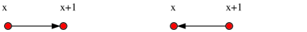
 $U_{\mu}(x)$  $U_{-\mu}(x+1)=U_{\mu}^{-1}=U_{\mu}^{\dagger}(x)$

Figure 2: The gluon field on the lattice.

This form for the gluon field makes it possible to maintain exact local gauge invariance on a lattice. To apply a gauge transformation to a set of gluon fields we must specify an SU(3) gauge transformation matrix at each point. Call this $G(x)$. Then the gluon field $U_{\mu}(x)$ simply gauge transforms by the (matrix) multiplication of the appropriate $G$ at both ends of its link. The quark field (a 3-dimensional colour vector) transforms by multiplication by $G$ at its site.

$$U_{\mu}^{(g)}(x) = G(x)U_{\mu}(x)G^{{\dagger}}(x+1_{\mu})$$

$$\psi^{(g)}(x) = G(x)\psi(x)$$

$$\overline{\psi}^{(g)}(x) = \overline{\psi}(x)G^{{\dagger}}(x).$$ (7)

To understand how this relates to continuum gauge transformations try the exercise of setting $G(x)$ to a simple U(1) transformation, $e^{i\alpha(x)}$, and show that Equation 7 is equivalent to the QED-like gauge transformation in the continuum, $A^{g}_{\mu}=A_{\mu}-\partial_{\mu}\alpha$.

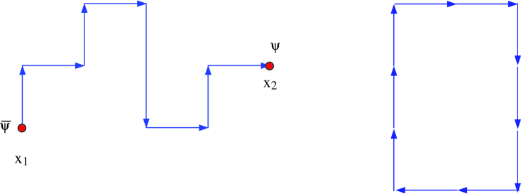
Figure 3: A string of gluon fields connecting quark and antiquark fields (left) and a closed loop of gluon fields (right).

Gauge-invariant objects can easily be made on the lattice out of closed loops of gluon fields or strings of gluon fields (Figure 3) with a quark field at one end and an antiquark field at the other, e.g. $\overline{\psi}(x_{1})U_{\mu}(x_{1})U_{\nu}(x_{1}+1_{\mu})\ldots U_{\epsilon}(x_{2}-1_{\epsilon})\psi(x_{2})$. Under a gauge transformation the $G$ matrix at the beginning of one link ‘eats’ the $G^{{\dagger}}$ at the end of the previous link, since $G^{{\dagger}}G=1$. The $G$ matrices at $x_{1}$ and $x_{2}$ are ‘eaten’ by those transforming the quark and anti-quark fields, if we sum over quark and antiquark colors. The same thing happens for any closed loop of $U$s, provided that we take a trace over color indices. Then the $G$ at the beginning of the loop and the $G^{{\dagger}}$ at the end of the loop, the same point for a closed loop, can ‘eat’ each other. (Try this as an exercise, remembering that $U$ fields going in the downward direction are $U^{{\dagger}}$s and, from Equation 7, $U_{\mu}^{{\dagger},(g)}(x)=G(x+1_{\mu})U_{\mu}^{{\dagger}}(x)G^{{\dagger}}(x)$.)

The purely gluonic piece of the continuum QCD action is

$$S_{\rm cont}=\int d^{4}x\frac{1}{4g^{2}}\mathop{\rm Tr}\nolimits F_{\mu\nu}F^{\mu\nu}$$ (8)

and the simplest lattice discretisation of this is the so-called Wilson plaquette action:

$$S_{\rm latt}=\beta\sum_{p}\left(1-\frac{1}{3}\mbox{Re}\,\{\mathop{\rm Tr}\nolimits U_{p}\}\right);\quad\beta=\frac{6}{g^{2}}.$$ (9)

$U_{p}$ is the closed $1\times 1$ loop called the plaquette, an SU(3) matrix

Figure 4: A plaquette on the lattice.

formed by multiplying 4 gluon links together in a sequence. For the plaquette with corner $x$ in the $i,j$ plane we have (Figure 4):

$$U_{p}(x)=U_{i}(x)U_{j}(x+1_{i})U^{{\dagger}}_{i}(x+1_{j})U^{{\dagger}}_{j}(x)$$ (10)

Tr in $S_{\rm latt}$ denotes taking the trace of $U_{p}$ i.e. the sum of the 3 diagonal elements. $S_{\rm latt}$ sums over all plaquettes of all orientations on the lattice. $\beta$ is a more convenient version for the lattice of the QCD bare coupling constant, $g^{2}$. This is the single input parameter for a QCD calculation (whether on the lattice or not) involving only gluon fields. Notice that the lattice spacing is not explicit anywhere, and we do not know its value until after the calculation. The value of the lattice spacing depends on the bare coupling constant. Typical values of $\beta$ for current lattice calculations using the Wilson plaquette action are $\beta\approx 6$. This corresponds to $a\approx$ 0.1fm. Smaller values of $\beta$ give coarser lattices, larger ones, finer lattices. Other improved discretisations of the gluon action are also used. In these the bare coupling constant appears in a different way and so comparison of the bare coupling constant between different gluon lattice actions is meaningless. The only comparison which makes sense is that of the resulting values for the lattice spacing. That $S_{\rm latt}$ of Equation 9 is a discretisation of $S_{\rm cont}$ is not obvious, and we will not demonstrate it here. It should be clear, however, from Equations 6 and 10 that $S_{\rm latt}$ does contain terms of the form $\partial_{\mu}A_{\nu}$.

$S_{\rm latt}$ is gauge-invariant, as will be clear from our earlier discussion. Thus lattice QCD calculations do not require gauge fixing or any discussion of different gauges or ghost terms. We simply calculate the appropriate Feynman Path Integral using $S_{\rm latt}$. Since we are only describing calculations for gluons at this stage, $\bm{\mathcal{O}}$ will be some gauge-invariant product of $U$ fields, for example the closed loop of Figure 3. Such a calculation is fully non-perturbative since the Feynman Path Integral includes all possible interactions in the matrix element that we are evaluating. In contrast to the real world, however, the calculations are done with a non-zero value of the lattice spacing and a non-infinite volume. In principle we must take $a\rightarrow 0$ and $V\rightarrow\infty$ by extrapolation. In practice it suffices to demonstrate, with calculations at several values of $a$ and $V$, that the $a$ and $V$ dependence of our results is small, and understood, and include a systematic error for this in our result.

2.3 Algorithms

The Feynman Path Integral (Equation 1) for gluons only becomes

$$\langle 0|\bm{\mathcal{O}}|0\rangle=\frac{{\displaystyle\int[dU]\,\bm{\mathcal{O}}e^{-S}}}{{\displaystyle\int[dU]\,e^{-S}}}.$$ (11)

To evaluate this integral we can generate random sets of $U$ fields on the lattice and work out the result:

$$\langle 0|\bm{\mathcal{O}}|0\rangle=\frac{{\displaystyle\sum\nolimits_{\alpha}\bm{\mathcal{O}}_{\alpha}e^{-S_{\alpha}}}}{{\displaystyle\sum\nolimits_{\alpha}e^{-S_{\alpha}}}}.$$ (12)

$\{U\}_{\alpha}$ is a set of $U$ matrices, one for each link of the lattice, and is called a configuration. $\bm{\mathcal{O}}_{\alpha}$ is the value of $\bm{\mathcal{O}}$ on that configuration (e.g. the trace of a closed loop of $U$s). A set of configurations is an ensemble.

This is a very inefficient way of working. If $S_{\alpha}$ is large for a particular configuration it contributes very little to the result. Instead it is better to generate the configurations with probability $e^{-S}$. This is called ‘importance sampling’ since we preferentially choose configurations with a large contribution to the integral. If we have a set of configurations so distributed then

$$\langle 0|\bm{\mathcal{O}}|0\rangle=\langle\bm{\mathcal{O}}\rangle=\frac{1}{N}\sum_{\alpha=1}^{N}\bm{\mathcal{O}}_{\alpha},$$ (13)

i.e. the result simply becomes the ensemble average of the value of the operator $\bm{\mathcal{O}}$ evaluated on each configuration. The calculation then has a statistical uncertainty associated with it, which varies with the ensemble size, $N$, as $1/\sqrt{N}$.

Several algorithms exist to generate an ensemble of configurations with distribution $e^{-S}$. The Metropolis algorithm is the earliest and simplest, but shares several features with later more sophisticated algorithms. The first step is to generate a starting configuration, $\{U\}_{1}$, e.g. by setting all the $U$ matrices to the unit $3\times 3$ matrix or by generating random SU(3) matrices. The algorithm then sweeps round the configuration, one $U$ matrix at a time. For each $U$ matrix a small change is proposed, i.e. a random matrix close to the unit matrix is generated which could multiply $U$. The change in $S$ is calculated if this change to $U$ were to happen. If $S$ is reduced, the change is accepted; if not, it is accepted with probability $e^{-\Delta{S}}$ (by comparing $e^{-\Delta{S}}$ to a random number between 0 and 1). Once this has been done for every $U\in\{U\}_{1}$ we have a new configuration, $\{U\}_{2}$. We then repeat to obtain $\{U\}_{3}$ etc. Once we have an ensemble we can do any number of different calculations (often called ‘measurements’) on it for different operators $\bm{\mathcal{O}}$. Ensembles are the equivalent of experimental data sets created by collaborations of theorists. They are often stored for years and re-used many times. Some ensembles are publicly available - see http://qcd.nersc.gov/ and http://www.ph.ed.ac.uk/ukqcd/.

An important point to note is that each member of an ensemble is generated from a previous member. The ensemble therefore has a (computer) time history. We have to worry about the ‘equilibration time’ and the ‘decorrelation’ (autocorrelation) time of the ensemble. The equilibration time is the number of sweeps required to reach a configuration typical of the distribution $e^{-S}$ that we are trying to create, i.e a configuration which has ‘forgotten’ the starting configuration. The autocorrelation time is the number of sweeps it takes to generate a sufficiently different configuration that results can be considered statistically independent. The autocorrelation time can be determined from the sequence of results for $\bm{\mathcal{O}}$ and will depend on $\bm{\mathcal{O}}$. In general if $\bm{\mathcal{O}}$ is an operator with large extent, e.g. a closed loop of $U$ fields over many lattice sites, it will have a longer autocorrelation time than if $\bm{\mathcal{O}}$ is a small loop. This is because the changes to a configuration spread out randomly from a point, one step per sweep. As we try to reach smaller values of $a$, closer to the continuous space-time of the real world, we expect a phenomenon called ‘critical slowing-down’. This is because a given physical distance, say the size of a hadron, takes up many more lattice sites as $a$ gets smaller. For an ensemble to decorrelate on this physical distance scale then requires more sweeps. This makes the numerical cost of reducing the lattice spacing at fixed physical volume far worse than the naïve $a^{4}$ (see Figure 5).

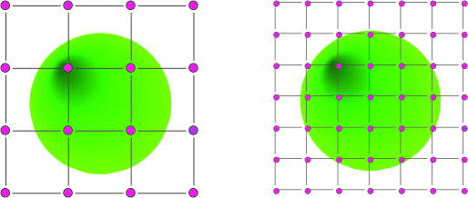
Figure 5: A given physical distance requires more lattice points to cover it as $a$ is reduced.

2.4 Quarks on the lattice

2.4.1 The fermion doubling problem

The inclusion of quarks in the lattice QCD action causes several difficulties related to their fermionic nature and makes lattice QCD calculations very costly in computer time.

The so-called ‘fermion doubling’ problem is apparent even for free quarks, in the absence of any interaction with the gluon field. The continuum action for a single flavor of free fermions is

$$S_{f}=\int d^{4}x\,\bar{\psi}(\gamma^{\mu}\partial_{\mu}+m)\psi.$$ (14)

The obvious (so-called naïve) lattice discretisation gives

$$S_{f}^{\rm latt,naive}=a^{4}\sum_{x}\left[\bar{\psi_{x}}\sum_{\mu=1}^{4}\gamma_{\mu}\frac{\psi_{x+1_{\mu}}-\psi_{x-1_{\mu}}}{2a}+m\bar{\psi_{x}}\psi_{x}\right].$$ (15)

The problems become evident when we Fourier transform this and compare the lattice inverse propagator:

$$G^{-1}_{\rm latt,naive}(p)=i\gamma_{\mu}\frac{\sin p_{\mu}a}{a}+m$$ (16)

to that obtained in the continuum from Equation 14,

$$G^{-1}_{\rm cont}(p)=i\gamma_{\mu}p_{\mu}+m.$$ (17)

The two are plotted for a massless quark in one-dimension in Figure 6 over one lattice Brillouin zone (momenta beyond $\pm\pi/a$ are equivalent to those in this range). The lattice result looks continuum-like around $p\approx 0$, where the inverse propagator is close to zero. The lattice inverse propagator is also close to zero around $p\approx\pi/a$, however. Since $\pi/a$ and $-\pi/a$ are periodically connected on the lattice, another continuum-like line can be drawn at this point (with opposite slope to the one at the origin). Thus in one-dimension, our lattice fermion contains two continuum-like fermions rather than one! On a 4-dimensional lattice we have $2^{4}$ fermions instead of one. The 15 excess fermions are called doublers. The doubling problem is clearly a consequence of the fact that the sine function appears in Equation 16 and this is because of the single derivatives in the Dirac action for a relativistic fermion, Equation 14. For a scalar particle (Equation 5) we would have a cosine instead, and no difficulty.

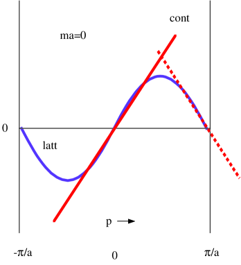
Figure 6: The doubling problem for lattice fermions. The sine curve shows the lattice quark inverse propagator in 1-d. The straight lines through $p$ = 0 (solid) and through $p=\pi/a$ (dotted) are those for a continuum quark.

2.4.2 Wilson quarks

There are several approaches to the doubling problem. The most severe in terms of its effects, but currently the most popular for a lot of applications, is the Wilson quark action. In this the doublers are entirely removed, by adding a ‘Wilson’ term to the action which gives them a much larger mass than $ma$, so that they drop out of the physics. The term added is a double derivative so appears with an extra power of $a$ ($a^{5}$) in order to have the same dimensions as the other terms in $S_{f}^{\rm latt}$ (Equation 15):

$$S_{f}^{W} = S_{f}^{\rm naive}-\frac{r}{2}a^{5}\sum_{x}\bar{\psi}_{x}\mbox{\Large$\Box$}\psi_{x},$$ (18)

$$\mbox{\Large$\Box$}\psi_{x} = \sum_{\mu=1}^{4}\frac{{\psi}_{x+1_{\mu}}-2\psi_{x}+\psi_{x-1_{\mu}}}{a^{2}},$$ (19)

where $r$ is the Wilson parameter (almost always set to 1). The extra power of $a$ in Equation 18 means that the correspondence between the lattice and continuum actions as $a\rightarrow 0$ is not changed. However, if we look at the inverse propagator again, there is a difference.

$$G^{-1}_{W}(p)=G^{-1}_{\rm naive}+\frac{2r}{a^{2}}\sum_{\mu=1}^{4}\sin^{2}(p_{\mu}a/2).$$ (20)

If we substitute for $G^{-1}_{\rm naive}$ from Equation 16 and expand out the $\sin$ function around $p\approx 0$ we get

$$G^{-1}_{W}(p)=i\gamma_{\mu}p_{\mu}+m+\frac{ra}{2}\sum_{\nu=1}^{4}p_{\nu}^{2}.$$ (21)

Comparing this to the continuum form (Equation 17) as $a\rightarrow 0$, the $r$ term will disappear and a fermion of mass $m$ will have the right form. If instead we look at the doublers, we must expand around $p\approx\pi/a$. If we call $\widetilde{p}$ the momentum difference between $p$ and $\pi/a$ and consider the case where $p$ has only one component close to $\pi/a$, and the others are close to zero, then

$$G^{-1}(\widetilde{p})=i\gamma_{\mu}\widetilde{p}_{\mu}+m+\frac{2r}{a}+\cdots\;.$$ (22)

Now as $a\rightarrow 0$, the mass of the doubler, $m+2r/a\rightarrow\infty$. The doublers at other corners of the Brillouin zone pick up masses of $4r/a,\;6r/a,\;8r/a$ : check this as an exercise. Thus we are assured that our quark action describes only the one quark that we intended, but there is a price for this, as we shall see below.

The Wilson quark action is converted to dimensionless units by a rescaling $a^{3/2}\psi\rightarrow\psi$, leaving the quark mass parameter as a mass in lattice units, $ma$ (previously called $m^{\prime}$).

$$S_{f}^{W}=\sum_{x}\left\{\bar{\psi}_{x}\sum_{\mu}\left[(\gamma_{\mu}-r)\psi_{x+1_{\mu}}-(\gamma_{\mu}+r)\psi_{x-1_{\mu}}\right]+(ma+4r)\bar{\psi}_{x}\psi_{x}\right\}.$$ (23)

It is conventional to define a ‘hopping parameter’ called $\kappa$ which is $1/(2ma+8r)$ and so $1/\kappa$ plays the rôle of the quark mass. $\psi$ is conventionally rescaled by $\sqrt{2\kappa}$ so that $\kappa$ moves to multiply the terms connecting the $\psi$ field on different sites (thus allowing ‘hops’). If we now couple in a gluon field, the $\psi$ field will become a 3(color)${\times}$4(spin) dimensional vector on each site. The gluon field must be included in such a way as to keep the action gauge-invariant. From our earlier discussion it is then obvious that $U$ matrices must be inserted as a link between the $\psi$ and $\overline{\psi}$ fields when they are on neighbouring sites. The Wilson quark action is then conventionally written:

$$S_{f}^{W}=\sum_{x}\left\{\kappa\left[\sum_{\mu}\bar{\psi}_{x}(\gamma_{\mu}-r)U_{\mu}(x)\psi_{x+1_{\mu}}-\bar{\psi}_{x+1_{\mu}}(\gamma_{\mu}+r)U_{\mu}^{{\dagger}}(x)\psi_{x}\right]+\bar{\psi}_{x}\psi_{x}\right\}.$$ (24)

The price we pay for using the Wilson quark action is that we break explicitly the chiral symmetry of continuum QCD. This is a symmetry of the derivative terms in $S_{f}$ (Equation 14) which allows us to rotate separately right- and left-handed components of the quark field. The spontaneous breaking of this symmetry gives us a massless pseudoscalar meson called the pion as a Goldstone boson and has other important consequences for particle physics. Chiral symmetry is broken explicitly by a quark mass (so that the real pion is not actually massless) but also, more seriously for the lattice, by the Wilson term. As $a\rightarrow 0$, chiral symmetry will be recovered, but for real lattice calculations at non-zero $a$, the lack of chiral symmetry can cause difficulties for some calculations.

One surprising feature of Wilson quarks is that it is still possible to get a massless pion even at non-zero $a$, when chiral symmetry is broken. However, we have to search for the value of $1/\kappa$ at which it occurs—it is not simply the point $1/\kappa=8r$, as it would be in the free theory, above. Lattice calculations of the mass of the pseudoscalar meson ($M_{\rm PS}$) must be done at various input values of $\kappa$ (see Section 3) for a given ensemble. A plot of $M_{\rm PS}^{2}$ against $1/\kappa$ is then extrapolated to the point where $M_{\rm PS}$ is zero. The value of $\kappa$ at this point is called $\kappa_{\rm critical}$ and is the point at which the bare quark mass in the interacting theory is zero (but matrix elements will not necessarily show chirally symmetric behaviour). The bare quark mass in lattice units, $ma$, at other values of $\kappa$ can then be taken to be $(1/2\kappa-1/2\kappa_{\rm critical})$.

Another problem for the Wilson quark action is the presence of large discretisation errors. The naïve quark action has discretisation errors proportional (at lowest power) to $a^{2}$ because (see Equations 16 and 17) $\sin(pa)/a=p(1-p^{2}a^{2}/6+\cdots)$. In the measurement of a hadron mass, the terms proportional to $p^{2}a^{2}$ in the action will induce an error proportional to $\Lambda^{2}a^{2}$ where $\Lambda$ is some typical momentum scale inside the hadron in question, say 300MeV. For lattice spacing values we can reach, around 0.1fm (= $(2{\rm GeV})^{-1}$ when $\mbox{$h$\raisebox{-0.04303pt}{${}^{-}$}}=c=1$), this gives an expected error of order 2%. The Wilson term (Equation 18) that we added, however, is proportional to $a$, so that $S_{f}^{W}=S_{f}^{\rm cont}+{{O}}(a)$. Now hadron masses will have an error of typical size $\Lambda a$, which could be 15% at $a$ = 0.1fm. One can extrapolate this error away by doing calculations at several values of $a$ but the size of the extrapolation adds uncertainty.

Instead, we can ‘improve’ the quark action, by adding additional terms to counteract the errors at any order in $a$. This is equivalent to a higher order discretisation scheme for differential equations. For the Wilson quark action we can add the so-called clover term, making the clover, or Sheikholeslami-Wohlerti, action:

$$S_{f}^{\rm clover}=S_{f}^{W}-\frac{iac_{\rm sw}\kappa r}{4}\sum_{x}\bar{\psi}_{x}\sigma_{\mu\nu}F_{\mu\nu}\psi_{x}.$$ (25)

The standard discretisation of $aF_{\mu\nu}$ is as a set of 4 plaquettes arranged in a clover-leaf shape. If the clover coefficient, $c_{\rm sw}$, is chosen correctly then the clover action has leading order errors proportional to $a^{2}$ again. It is in the correct choice of this coefficient that the difficulties of discretising a field theory, as opposed to a standard differential equation, appear. We are trying to match QCD with an ultraviolet momentum cut-off of $\pi/a$ to QCD with an infinite momentum cut-off. Gluonic interactions with gluon momenta between $\pi/a$ and $\infty$ in the continuum must be accounted for on the lattice by a renormalisation of coefficients in the action. Thus the naïve (tree-level) value of 1 for $c_{\rm sw}$ is renormalised by an amount which depends on the QCD coupling constant at some momentum scale around $\pi/a$. This momentum scale is typically quite large (for $a$ = 0.1fm it is 6GeV) so that a perturbative calculation of $c_{\rm sw}$ can work well. $c_{\rm sw}=1+c_{1}\alpha_{s}(\pi/a)+c_{2}\alpha_{s}^{2}(\pi/a)+\cdots\,$. In fact it has been shown that a lot of the perturbative correction can be absorbed into a renormalisation of the $U$ field by a factor called $u_{0}$, and this is called tadpole-improvement (Lepage, 1993). Alternatively $c_{\rm sw}$ can be determined within the lattice calculation itself (i.e. non-perturbatively) by insisting that some continuum relationship, broken by the discretisation errors, works on the lattice (Sommer, 1998). For $c_{\rm sw}$ we can impose Ward identities from chiral symmetry, for example. This improvement programme for the lattice action can be carried further at the cost of introducing more coefficients that have to be determined by a match to continuum QCD. However, this must be compared to the cost of not improving the action, which requires calculations on very fine lattices to achieve small enough discretisation errors for the accuracy we require and is generally prohibitive.

2.4.3 Staggered quarks

Here we return to the naïve quark action and ask, what was so bad about having 16 quarks instead of 1? If we had 16 flavors of quarks of the same mass in Nature, the naïve action might be fine. In fact we only have two quarks that might be considered degenerate, $u$ and $d$. They both have masses of a few MeV. Although we do not believe that their masses are the same, the difference is much smaller than any other mass, and they are treated as degenerate in most lattice calculations at present.

We can ‘thin’ the degrees of freedom of the naïve lattice quark action by removing the 4 spin degrees of freedom (which can be shown to be multiple copies of the same thing). The quark field, $\chi$, then becomes a 3(colors)$\times$1(spin) component object on a site and the staggered (Kogut-Susskind) fermion action is:

$$S_{f}^{S}=\sum_{x}\bar{\mbox{\raisebox{1.72218pt}{$\chi$}}}_{x}\left\{\frac{1}{2}\sum_{\mu}\eta_{x,\mu}\left(U_{\mu}(x)\mbox{\raisebox{1.72218pt}{$\chi$}}_{x+1_{\mu}}-U_{\mu}^{{\dagger}}(x-1_{\mu})\mbox{\raisebox{1.72218pt}{$\chi$}}_{x-1_{\mu}}\right)+ma\mbox{\raisebox{1.72218pt}{$\chi$}}_{x}\right\}.$$ (26)

$\eta_{x}$ is $\pm 1$ according to the formula $\eta_{x,\mu}=(-1)^{k}$ where $k={\sum_{\nu<\mu}x_{\nu}}$. This action describes 16/4 = 4 quarks, now much closer to the real world, if we want to interpret the doublers as flavors. We might hope that if the 4 flavors do behave as 4 copies of the same thing we can reduce their effect by a factor of two or four (depending on how many degenerate flavors we want to simulate) by multiplication with the required factor at appropriate points (as we could in QCD perturbation theory). The 4 spin degrees of freedom for the 4 flavors are made from the 16 components of the $\chi$ field on a $2^{4}$ hypercube, which is a complication if we need to separate out the flavors. The staggered action, however, has a remnant of chiral symmetry which ensures the very desirable feature that the quark mass (and the associated Goldstone boson pion mass) vanish at $ma$ = 0. This behaviour gives the added benefit of making staggered quarks rather better behaved and computationally much faster to work with than Wilson-type quarks.

The down-side of staggered quarks is again the discretisation errors. These are formally ${O}$$(a^{2})$, just as for naïve quarks, but some of the errors induce flavor-changing interactions and so are rather dangerous. In practice they produce a larger than expected effect for simple $a^{2}$ errors. A quark with momentum around 0 can be scattered to one with momentum around $\pi/a$ i.e a doubler, and therefore a different flavor, by the interaction of Figure 7. One of the results of this is that the 16 different pions (for 4 flavors) no longer have the same mass and only one of them has a mass which vanishes as $ma\rightarrow 0$. Improvement terms have recently been developed which can be added to the action to reduce these interactions to a much lower level, and the masses of the different pions are then much closer together (Bernard, 2001, MILC collaboration). This makes the prospects for working with staggered quarks in lattice QCD calculations much better, and a lot more work with these quarks will certainly be done.

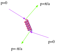
Figure 7: A flavor-changing interaction for staggered quarks on the lattice.

2.4.4 Ginsparg-Wilson quarks

A recent development has been a set of quark actions which maintain chiral symmetry of the action while still describing only one quark flavor, but at the cost of a very complicated lattice discretisation of the continuum derivative. This is then costly to implement. For example, in the domain-wall formulation an additional 5th dimension is required whose length, in principle, must go to infinity. A lot of work is being done to develop algorithms for these quark actions which may make them feasible in the long-term. In the meanwhile, they are already being used for calculations that really need chiral symmetry at finite lattice spacing, such as that of the CP-violating parameter in the $K$ system, $\epsilon^{\prime}$.

2.5 Algorithms for quarks

Another problem with handling quarks in lattice QCD is that they are fermions, obeying the Pauli Exclusion Principle, and therefore cannot be represented by ordinary numbers in a computer. We must do the quark functional integral by hand:

$$\int[dU]\,[d\psi]\,[d\bar{\psi}]\,e^{-S_{g}+\bar{\psi}M\psi}=\int[dU]\,{\det}Me^{-S_{g}}$$ (27)

where the form for the matrix $M$ depends on the quark formulation and can be derived from the forms given above for the quark action (Equations 24, 25 and 26). The QCD action then becomes

$$S=\beta\sum_{p}\left(1-\frac{1}{N_{c}}\mbox{Re}\,\mathop{\rm Tr}\nolimits\left(U_{p}\right)\right)-\ln\left(\det M\right).$$ (28)

We now generate ensembles of gluon fields (only) with importance sampling based on this action. The standard algorithm for doing this is called Hybrid Monte Carlo . The second term is a very expensive one to include, because it requires frequent calculations of $M^{-1}$ (various algorithms, such as Conjugate Gradient exist to do this) and $M$ is a large matrix ($4{\rm(forWilson)}\times 3\times V\approx 2\times 10^{6}$ on a side). If this term is missed out for expediency (so that the action is just $S_{g}$) then we talk of using the ‘quenched approximation’. Most calculations in the past have been quenched (and most of the results I discuss later will be in the quenched approximation) but recently calculations using the full QCD action (‘unquenched’ or ‘with dynamical/sea quarks’) have been attempted and in the future we hope that the quenched approximation will become redundant. We can think of the $\ln(\det M)$ term as giving rise to a sea of quark/anti-quark pairs appearing and disappearing in the vacuum. For every quark flavor for which we have a separate matrix $M$ we should in principle include a term of the form $\ln(\det M)$ in the dynamical quark action. However, it is only the production of light ($u,d,s$) quark/anti-quark pairs that we envisage having a significant effect for most of the quantities that we calculate. Dynamical lattice calculations are then done with $N_{f}$ = 2 for $u,d$ dynamical quarks or 2+1 if $s$ is included.

Quarks must also be integrated out of the operators, $\bm{\mathcal{O}}$. For $\bm{\mathcal{O}}=(\overline{\psi}\psi)_{y}(\overline{\psi}\psi)_{x}$, the form mentioned earlier, which creates a meson at the point $x$ and destroys it at the point $y$, then

$$\int[dU][d\psi][d\bar{\psi}]\bar{\psi}^{u,a}_{y}\psi^{d,a}_{y}\bar{\psi}^{d,b}_{x}\psi^{u,b}_{x}e^{-S}=\int[dU](M^{-1,u}_{x,y}[U])^{ab}(M^{-1,d}_{y,x}[U])^{ba}{\rm det}Me^{-S_{g}}.$$ (29)

$M^{-1}$ is the quark propagator from $x$ to $y$ on a given gluon configuration, obtained by solving $Mx=b$ where $b$ is a vector with a 1 at $x$ (and a certain color and spin index) and $0$ everywhere else. We have been explicit here about the flavor indices, which we have taken as $u$ and $d$, although lattice calculations usually then assume that $u$ and $d$ are degenerate and therefore the two $M^{-1}$ factors are the same. However, if the hadron actually does contain two quarks of the same flavor then ‘disconnected’ pieces containing $M^{-1}_{x,x}$ will appear, as well as the ‘connected’ pieces above. The color indices, $a$ and $b$, are also explicit (and summed over) and make $\bm{\mathcal{O}}$ gauge-invariant. The sums over spin indices have not been made explicit because in this case they follow the color indices (but see Section 2.6). On an importance-sampled ensemble (either quenched or unquenched) for this example we then have to calculate ${\rm Tr_{\rm color,spin}}(M^{-1,u}_{x,y})(M^{-1,d}_{y,x})$ on every configuration and average over configurations.

Calculating $M^{-1}$ is computationally expensive and gets harder as $M$ develops small eigenvalues, which happens as $ma\rightarrow 0$ (for staggered quarks) or $\kappa\rightarrow\kappa_{\rm crit}$ (for Wilson or clover quarks). Thus, even in the quenched approximation, we cannot actually calculate with quark masses close to those of real $u$ and $d$ quarks. Instead we work with heavier quarks and perform so-called chiral extrapolations to the chiral limit where $u$ and $d$ quarks would be (almost) massless.

2.6 Relating lattice results to physics

Above we have given an example for $\bm{\mathcal{O}}$, which includes the creation of a valence quark and anti-quark at the point $x$ and their destruction at the point $y$. This is a so-called hadron correlator or 2-point function on the lattice since it simply has a source and a sink, and is one of the simplest quantities to calculate. It is shown pictorially at the left of Figure 8, where the solid lines indicate the valence quark propagators, and the blobs at the two ends indicate the creation and annihilation of the meson. A baryon would of course have 3 valence quark propagator lines. Usually we project onto specific values of $\mathbf{p}$ for the hadron, so in Figure 8 we have suppressed spatial indices at the source and sink and just refer to the time index, $0$ at the source and $T$ at the sink. The figure shows how, as the valence quarks propagate, they interact any number of times by exchange of gluons. This is a pictorial representation of the fully non-perturbative nature of a lattice QCD calculation. The interactions include the production of dynamical quark/anti-quark pairs if a dynamical calculation is being done.

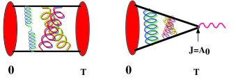
Figure 8: A graphical representation of two types of 2-point functions calculated on the lattice. Left, that for a hadron mass calculation; right, that for a decay constant.

The calculation of this 2-point function will enable the extraction of the hadron mass (see below), for the hadron corresponding to the $J^{PC}$ quantum numbers of $\bm{\mathcal{O}}$. We make different quantum numbers by inserting $\gamma$ matrices between the $\psi$ and $\overline{\psi}$ fields in each piece of $\bm{\mathcal{O}}$. For example, $(\overline{\psi}\gamma_{5}\psi)_{x}$ creates a pseudoscalar meson (such as $\pi$) and $\overline{\psi}\gamma_{i}\psi$ a vector (such as $\rho$). When the quark functional integral is done, as in Equation 29, $\gamma$ matrices will appear between the two $M^{-1}$ factors and appropriate sums over spin indices will have to be done.

The blobs in Figure 8 indicate that we can use more complicated forms for $\bm{\mathcal{O}}$ for a given hadron, e.g. the $\psi$ and $\overline{\psi}$ fields do not both need to taken at the point $x$. We can separate them spatially, either by inserting $U$ fields to keep $\bm{\mathcal{O}}$ gauge-invariant, or by fixing a gauge to allow spatial separation without including $U$ fields. This enables us to feed in information, or prejudice, about the relative spatial distribution of the quarks in the hadron, i.e. its ‘wavefunction’. Each piece of $\bm{\mathcal{O}}$ takes the form $\overline{\psi}_{x+r}\phi(r)\psi_{x}$ (suppressing the $U$ fields) where $\phi$ is some function of the separation between $\psi$ and $\overline{\psi}$: it is known as the ‘smearing’ function and $\bm{\mathcal{O}}$ is then a smeared operator. When the quark functional integral is done, factors of $\phi$ will appear between the $M^{-1}$ factors. The factor of $\phi$ is absorbed at the source by solving $Mx=\phi$ for, say, the quark (making a ‘smeared quark propagator’) and $Mx=\delta$ for the anti-quark (a ‘local quark propagator’). The two propagators are then put together with an explicit insertion of $\phi$ at the sink. Often calculations measure separately hadron correlators with several different smearing functions at both source and sink, enabling a more precise determination of the hadron mass.

Another type of 2-point function is shown on the right of Figure 8. In this case we create the hadron with a smeared operator and destroy it with a local operator. This is a ‘smeared-local’ or ‘smeared-current’ correlator, since the quantity that we can extract from this is the matrix element of the appropriate current operator, $J$, between the vacuum and the hadron. For example, this is used to calculate the decay constant, $f_{\pi}$, related to the vacuum to $\pi$ matrix element of the axial vector current (denoted by its time component, $A_{0}$, in Figure 8). This couples to the $W$ particle and mediates the purely leptonic decay of a $\pi$ meson. See the Lagrangian for the weak interactions in (Rosner, 2002), but note that the $W$ particle is not included explicitly in lattice QCD calculations. $\bm{\mathcal{O}}$ in this case then takes the form $(\overline{\psi}_{x+r}\gamma_{5}\phi(r)\psi_{x})(\overline{\psi}\gamma_{0}\gamma_{5}\psi)_{y}$, where the first factor creates the pion with a smeared operator at $x$ and the second destroys it with the time component of the local axial vector current. The quark functional integral converts this to the same type of quantity, with two factors of $M^{-1}$, that we discussed above.

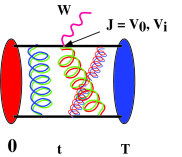
Figure 9: A graphical representation of a 3-point function (for semileptonic decay) calculated on the lattice.

Figure 9 shows a lattice 3-point function appropriate to the semi-leptonic decay of a hadron. One of the valence quark lines emits a $W$ and changes to a different flavor. A new hadron is then formed with the spectator quark. The emission of the $W$ can be represented by the insertion of a current on one of the valence quark lines. The Figure shows a vector current (with temporal component $V_{0}$ and spatial component $V_{i}$) which contributes to the decay of a pseudoscalar meson to a pseudoscalar meson (e.g. $B\rightarrow D$). We then have a (smeared) source and sink at $0$ and $T$, and a (local) current insertion at $t$, i.e. 3 points. When the quark functional integral is done there will be 3 factors of $M^{-1}$, one for the original valence quark which decays (from 0 to $t$), one for the final valence quark (from $t$ to $T$) and one for the spectator (from 0 to $T$). In fact the most efficient way to do this calculation is to solve for the final valence quark propagator from $T$ to $t$, taking as a source the spectator quark propagator from 0 to $T$.

3 Lattice QCD calculations

3.1 The steps of a typical lattice calculation

Step 1

A volume and a rough lattice spacing are chosen. A volume of $(3{\rm fm})^{3}$ is considered to be large enough not to ‘squeeze’, and therefore distort, typical hadrons placed on it. The time extent is usually taken as twice the spatial size since masses etc are extracted from the time dependence of hadron correlators (see below). The selection of the lattice spacing is a trade-off between getting close to the continuum limit (and therefore small discretisation errors) and the cost of the calculation, which grows as some large power of $a^{-1}$. Improvement of the action, discussed above, helps here by giving small discretisation errors on coarser lattices. Lattice spacings around 0.1fm are reasonable on both counts. From experience we know roughly what value of the bare QCD coupling constant to take in the gluon part of the QCD action to achieve various values of $a$ (determined after the calculation, see below). However, the quark contribution to the action affects this also, and we have much less experience with this. A $(3{\rm fm})^{3}\times 6{\rm fm}$ lattice with $a\approx$ 0.1fm requires $(30)^{3}\times 60$ sites.

Step 2

A quark formulation, number of quark flavors, and masses in lattice units, $ma$, are chosen for the quark part of the QCD action. Again we have a trade-off between trying to take realistically small masses for the $u$ and $d$ quarks, and the cost. Again we do not know what the quark mass actually is until after the calculation, when we have calculated the masses of hadrons containing that quark. Recent calculations have been able to take dynamical quark masses down to the $s$ quark mass and some have gone further; future calculations need to reach much smaller masses than this. Extrapolations to $u$ and $d$ quark masses will continue to be necessary, however (see step 8). Some interpolation will always be necessary too since the masses chosen will inevitably not be exactly correct, e.g. for the physical strange quark mass.

Step 3

An ensemble of gluon configurations must then be generated using importance sampling with $e^{-S}$. As discussed above, dynamical quarks appear implicitly through the quark determinant.

Step 4

Quark propagators are calculated on each gluon configuration of the ensemble by inverting the quark matrix, $M$, to make the ‘valence’ quarks inside the hadron. Where they are supposed to have the same flavor as the dynamical quarks, they should have the same mass in lattice units, $ma$. However, we can also calculate valence quark propagators for quarks with different mass from the dynamical quarks, and perform separate extrapolations in valence and dynamical quark masses. This is sometimes useful and particularly so if there is a very limited set of dynamical quark masses. It is known as the partially quenched approximation (PQA).

Step 5

The quark propagators are then put together in various combinations to form hadron correlators (see the discussion of the form taken for operators, $\bm{\mathcal{O}}$, above) which are then averaged over all the configurations in the ensemble. We are concentrating here on operators $\bm{\mathcal{O}}$ which are related to quark-based hadrons but gluonic operators can also be measured on the ensemble and averaged in the same way.

Step 6

The hadron correlators are fitted to their expected theoretical form to extract hadron masses and matrix elements. For the 2-point function described for the spectrum, the ensemble average of the product of smeared quark propagators described above gives us the vacuum expectation value of a hadron correlator, $\langle 0|H^{{\dagger}}(T)H(0)|0\rangle$ (see Equation 1). The hadron creation(destruction) operator can create(destroy) from the vacuum all the hadron states which have the same $J^{PC}$ quantum numbers as the operator. For example, if the operator has the quantum numbers of a pseudoscalar meson containing $u$ and $d$ quarks, the $\pi$ and all its radial excitations can be created(destroyed). The amplitude, $A$, with which a particular state is created or destroyed depends on the overlap with that state of the operator used, i.e. the smearing function, at source or sink. Thus we obtain

$$\langle 0|H^{{\dagger}}(T)H(0)|0\rangle=\sum_{n}\frac{A_{{\rm src},n}A_{{\rm snk},n}}{2E_{n}}e^{-E_{n}T}$$ (30)

where the factor $e^{-E_{n}T}$ arises because the two hadron operators are offset by a time distance $T$ in Euclidean space, and $E_{n}$ is the energy of the $n$th state. The states which dominate the fit, especially at large values of $T$, are those with lowest energy; if a projection on zero momentum has been done, these will be the states with lowest mass. Often we are interested in the one state with lowest mass, the ground state (the $\pi$ in the example above), and then try to design a good smearing function to have large overlap with that state, and very small overlap with its radial excitations. In that case fits can be done in which data at small values of $T$ are thrown away and only a single exponential is used in the fit. The extent to which this works can be gauged by plotting the ‘effective mass’, the log of the correlator at time $t$ divided by $t$. If one state completely dominates the fit, a constant result is obtained as a function of $t$ - the effective mass is said to ‘plateau’. The plateau value is the ground state mass. Figure 10 shows the result for the effective mass of the correlator for an $\Upsilon$ particle (see Section 4) calculated on the lattice. A clear plateau is seen but only for $t>$ 15. For smaller $t$ the correlator clearly contains excitations of higher mass, because no smearing was used in this case.

The best calculations use several different smearing functions at source and sink and perform simultaneous multi-exponential fits of the type in Equation 30. If the masses of several states can be obtained from the fit the reliability of the ground state mass is increased. It should also be pointed out that correlated fitting techniques must be used since the correlators at adjacent times are not statistically independent of each other.

Figure 10: The effective mass of a $1^{--}$ $b\overline{b}$ ($\Upsilon$) correlator, calculated from a lattice 2-point function with local source and sink.

For the 2-point function used to calculate decay constants, the amplitude with which the hadron is destroyed at the sink is the vacuum to hadron matrix element of the current.

$$\langle 0|J(T)H(0)|0\rangle=\sum_{n}\frac{A_{{\rm src},n}\langle 0|J|n\rangle}{2E_{n}}e^{-E_{n}T}$$ (31)

and $\langle 0|A_{0}|\pi(\mathbf{p}=0)\rangle=f_{\pi}m_{\pi}$. To isolate the part proportional to the decay constant requires dividing the total amplitude of the ground state exponential by $A_{{\rm src},n=g.s.}$. This can be obtained from a fit of the type in Equation 30, if the same smearing function is used at source and sink so that $A_{{\rm src},n}=A_{{\rm snk},n}$.

For the 3-point function we have two sets of hadrons with different flavor quarks, separated by a current insertion.

$$\langle 0|H^{\prime{\dagger}}(T)J(t)H(0)|0\rangle=\sum_{n}\sum_{m}\frac{A_{{\rm src},n}A_{{\rm snk},m}\langle m|J|n\rangle}{2E_{n}2E_{m}}e^{-E_{n}t}e^{-E_{m}(T-t)}$$ (32)

where $n$ runs over hadrons with the quantum numbers of the operator at 0 and $m$, those of the operator at $T$. Again the matrix element of interest, that of the current between two hadrons (usually for the ground states in the two cases), can be obtained by dividing out the amplitudes at source and sink from two separate 2-point fits for the two different hadrons of the kind in Equation 30.

Step 7

It is now possible to determine what the lattice spacing was in the simulation. This then sets the single dimensionful scale so that everything can be converted to physical units (GeV) from lattice units. The lattice spacing is determined by requiring one dimensionful quantity to take its real world value. Usually a hadron mass is chosen, because these are easiest to determine on the lattice, but it should not be one whose mass depends strongly on valence quark masses to be determined in the next step (see below) otherwise a complicated iterative tuning procedure will result. The most popular quantity to use at present is known as $r_{0}$, a parameter associated with the potential between two infinitely heavy quarks. It is extracted from the energy exponent of a gluonic operator (the closed loop of Figure 3), so can be precisely determined and does not contain any valence quark masses. The only problem is that it is not an experimentally accessible quantity, and we rely on potential model results to give a phenomenological value, estimated to be 0.5fm. Another quantity frequently used is the mass of the $\rho$ meson, obtained by chiral extrapolation to the point where the $\pi$ meson mass, and therefore the $u$,$d$ quark mass, is (almost) zero. The chiral extrapolation, however, can produce large errors. A better quantity is the orbital excitation energy, i.e the splitting between P states and S states, in $b\overline{b}$ or $c\overline{c}$ systems, since these don’t contain light quarks and this splitting is even insensitive to the heavy quark mass. (The treatment of heavy quarks on the lattice will be discussed in Section 4.)

Step 8

The step above yields all hadron masses in GeV. However, before we can compare to experiment we must tune the quark masses. This requires calculations at several different values of the bare quark masses in an appropriate region. For each quark mass we then select a hadron whose mass will be used for tuning (and is therefore not predicted). For that hadron we interpolate/extrapolate the results to find the bare quark mass at which that hadron mass is correct. The masses of other hadrons containing that quark are then predicted if we interpolate/extrapolate those masses to the same quark mass, or combination of quark masses. In the process we learn about the dependence of hadron masses on the quark mass and this can be useful theoretical information. The hadrons used for tuning should be low-lying states with accurate experimental masses which can be calculated precisely on the lattice. The $\pi$ mass is usually used to fix the $u$, $d$ mass (taken to be the same), although sometimes the approximation $m_{\pi}=0$ is used. The mass of the $K$, $K^{{{\displaystyle*}}}$, or $\phi$ can be used to fix the $s$ quark mass. The $K$ or $K^{{{\displaystyle*}}}$ obviously require the $u$ and $d$ masses to have been fixed. The dimensionless ratio of the $K^{{\displaystyle*}}$ to the $K$ mass can also be used, and this is then less dependent on the quantity used to fix the lattice spacing. For the $c(b)$ quarks, the $D(B)$, $D_{s}(B_{s})$ or $\psi(\Upsilon)$ systems are convenient ones.

The interpolation/extrapolation of hadron masses as a function of bare quark masses is a relatively simple procedure in the quenched approximation. Then there is no feedback from the quark sector into the gluon sector. We can create gluon field configurations at a fixed value of the lattice spacing (as determined, for example, from a purely gluonic quantity such as $r_{0}$) and measure hadron masses at many different quark masses on those configurations. The issues are then the correlations between results at different quark masses that must be taken into account and the spurious non-analytic behaviour in quark mass that can arise in the quenched approximation in extrapolations to $u$ and $d$ masses (‘quenched chiral logarithms’).

When we include dynamical quarks in the calculation, the effects of the quark determinant at a particular quark mass feed into the gluon field configurations. Results at different dynamical quark masses then represent a completely new calculation, generating a new ensemble of gluon configurations with statistically independent results. The interpolations/extrapolations in quark mass take on a new dimension and there are subtleties associated with how to do this. Some groups have chosen to generate configurations at fixed bare coupling constant and various dynamical bare quark masses. Then the lattice spacing will vary with quark mass and extrapolations in quark mass must be done in lattice units, before fixing the lattice spacing at the end. I believe a more satisfactory approach from a physical perspective is to adjust the bare coupling constant at different bare quark masses so that the lattice spacing remains approximately the same (as determined from $r_{0}$, for example). This then allows interpolations/extrapolations for physical hadron masses, and a better picture of the physical dependence of quantities on the presence of dynamical quarks. Several groups have also carried out this procedure.

In all of these approaches we must extrapolate to reach the physical $u/d$ mass region, and so we need to know the appropriate functional form for this extrapolation. This can be derived for light enough $u/d$ mass using an effective theory of Goldstone pions called chiral perturbation theory. This shows that logarithmic behaviour of quantities as a function of the $\pi$ mass (the variable representing the $u/d$ quark mass) should be present in general as well as simple power-law behaviour. These ‘chiral logarithms’ will only show up at rather small quark masses ($m_{u,d}\stackrel{{\scriptstyle<}}{{\sim}}m_{s}/4$) and so it is important for dynamical simulations to reach quark masses low enough to be able to match on to this behaviour and extrapolate down.

Step 9

The calculation needs to be repeated at several values of the lattice spacing to check that the dependence of physical results on the lattice spacing is at an acceptable level and/or to extrapolate to the continuum limit $a=0$. Extrapolations again obviously require knowledge of an appropriate functional form.

Step 10

Compare to experiment or give a prediction for experiment!

Concluding remark

Above we have described an ideal situation. Lack of computer power has meant compromising on one or more aspects in existing calculations. A lot of calculations have used the quenched approximation. More recent dynamical calculations have used heavy dynamical masses on rather coarse and sometimes rather small lattices. These difficulties should be overcome in the next few years and this will represent a huge improvement in the reliability of lattice results.

3.2 Control of lattice systematic errors

We aim for errors of a few percent from future lattice calculations. This requires both improved statistical errors in general and good control of systematic errors. Improved statistical accuracy is obtained by generating larger ensembles of configurations with a cost proportional to the square of the improvement. Improved systematic accuracy requires theoretical understanding of the sources of error and how to remove them. It is this understanding, described below, that has been responsible for the development of good lattice techniques and the convergence of lattice results in the quenched approximation through the late 1990s. This must be carried further in the next phase of dynamical simulations to reach the goal of providing quantitative tests of QCD and input to experiment.

3.2.1 Discretisation errors

As discussed earlier, these arise from errors in the lattice form of the Lagrangian, and operators $\bm{\mathcal{O}}$, compared to the continuum versions. Lattice results, even when converted to physical units, have some dependence on $a$. This will be as a power series in $a$, starting at $a^{n}$. As discussed earlier, $n$ = 1 if the Wilson quark action is used, 2 for the clover quark action and 2 for the staggered quark action. $n$ is also 2 for the Wilson plaquette gluon action of Equation 9. We expect the size of the $a$ dependence to be controlled by a typical momentum scale relevant to the quantity being calculated. Quantities sensitive to shorter distances than others will be more susceptible to discretisation errors, even though the value of $n$ depends only on the action used. Improved gluonic and quark actions are available in which higher order terms are added to $\cal{L}$ to increase $n$, and therefore reduce the $a$ dependence, and these can be tested for their efficacy in the quenched approximation. The systematic improvement method is known as Symanzik improvement (Gupta, 1998).

Figure 11: A scaling plot in the quenched approximation for the vector meson at a quark mass such that the pseudoscalar meson has mass $m_{\pi}r_{1}=0.807$. The vector meson mass is given in units of $r_{1}$, a variant of $r_{0}$, where $r_{1}\approx$ 0.35fm $=0.57{\rm GeV}^{-1}$. It is plotted versus the square of the lattice spacing, also given in units of $r_{1}$. The squares and fancy diamonds use an improved gluon action; the others use the Wilson plaquette action. The quark actions used are: circles, staggered (Kogut-Susskind); squares, improved staggered; fancy squares and fancy diamonds, tadpole-improved Wilson (clover); diamonds, Ginsparg-Wilson (domain wall). (Toussaint, 2002)

Figure 11 shows a scaling plot of the vector meson mass (the $\rho$, except that the quark mass is heavier than the real $u,d$ mass) in GeV versus the lattice spacing for various quark actions (Toussaint, 2002). Some of the calculations use an improved gluon action, with discretisation errors reduced beyond ${O}$$(a^{2})$, but others use the Wilson plaquette action. There is very little difference between these (compare fancy diamonds and squares) so that most of the difference arises from the quark action used. A variant of $r_{0}$, called $r_{1}$, is used to set the lattice spacing so the vector mass and scale are given in units of $r_{1}$. The plot shows results for clover quarks (improved Wilson quarks), staggered quarks, improved staggered quarks and Ginsparg-Wilson (domain wall) quarks. The last two formulations, which are both improved to remove ${O}$$(a^{2})$ errors show an impressively flat line, i.e. very little $a$ dependence for this quantity. The clover quarks shown here have a clover improvement coefficient (see Section 2.4.1) chosen using tadpole-improvement. This reduces the $a$ dependence of Wilson quarks to $\alpha_{s}a$ but it is clearly still visible. A non-perturbative determination of the clover improvement coefficient can reduce the $a$ dependence further to ${O}$$(a^{2})$, and then this formulation looks rather better. Notice the large discretisation errors visible for unimproved staggered quarks, despite the fact that the errors are ${O}$$(a^{2})$ (and results therefore lie on a straight line in the Figure). Provided that all the different quark formulations have been fixed to the same physical quark mass, all the results for the vector meson mass should agree in the $a\rightarrow 0$ limit. This does seem to be true, within the statistical errors shown.

3.2.2 Finite volume

Lattice results will be distorted if the space-time box in which the calculation is done is too small to adequately represent the infinite space-time volume of the real world. For large enough volumes the error should be exponential in the lattice size, $\propto e^{-ML}$, for a lattice of size $L$ in physical units. This means that it is possible to reduce finite volume errors rapidly to zero by taking large enough volumes. The lightest particle is the $\pi$, so this sets the volume required as we reduce the $u,d$ quark masses to their physical values. For $u,d$ quark masses of $m_{s}/4$, $m_{\pi}L>5$ for $L>$ 3fm, giving a finite volume error of less than 1%. Most recent lattice calculations have used volumes of this size, although there has been little systematic dependence of the volume dependence of results.

3.2.3 Matching hadronic matrix elements to the continuum

The calculation of hadronic matrix elements of various currents, $J$, on the lattice is discussed for 2- and 3-point functions in Section 2.6. An important point is that these depend in general on how QCD has been regularised and a finite renormalisation is then required to convert lattice results to those appropriate to a continuum scheme (such as $\overline{MS}$). Since lattice QCD and continuum QCD differ in the ultra-violet (for momenta greater than $\pi/a$), this renormalisation can be calculated in perturbation theory, by matching the matrix elements of $J$ between quark states. We usually need several lattice currents to make up the continuum current and a mixing and matching calculation must be done.

$$J_{\rm cont} = Z_{0}J_{\rm latt}^{(0)}+aZ_{1}J_{\rm latt}^{(1)}+\cdots$$

$$Z_{i} = 1+c^{(1)}_{i}\alpha_{s}(2/a)+c^{(2)}_{i}\alpha_{s}^{2}(2/a)+\cdots$$ (33)

Lattice perturbation theory is done in the same way as continuum perturbation theory, in terms of the field $A_{\mu}$ and including gauge-fixing and ghost terms, if necessary. Relatively little lattice perturbation theory has been done up to now and few results exist beyond ${O}$$(\alpha_{s})$. This leaves errors of ${O}$$(\alpha_{s}^{2})$, 5–10% if we take a scale for $\alpha_{s}$ of $2/a$ at $a{=}0.1$fm. Higher order calculations will be required to reduce this to the required level of 2–3%, and techniques are being developed to do this. It is also sometimes possible to fix the normalisation of lattice currents non-perturbatively using symmetry arguments or to match numerically between lattice and continuum $MOM$-type schemes. In whatever way it is done, the matching of lattice matrix elements to the continuum is a lot of work and an area where improvements are still necessary.

3.2.4 Unquenching

The neglect of dynamical quarks in the quenched approximation is obviously wrong, but how wrong? For many years systematic errors from the quenched approximation were obscured by the size of the statistical and discretisation errors. Now improved quenched calculations are showing internal inconsistencies and disagreement with experiment which we believe will be removed once realistic dynamical calculations can be done.

One effect expected in the quenched approximation is the incorrect (too fast) running of the coupling constant from one scale to another because of the absence of $g\rightarrow\overline{q}q\rightarrow g$ pieces in the vacuum polarisation to give quark screening of the color charge. From this we might expect that the determination of the lattice spacing would depend on the quantity used to fix it, since different quantities will be sensitive to different distance/momentum scales and these will not be connected correctly by the running of $\alpha_{s}$ in the quenched approximation. (Using a quantity to fix $a$ is equivalent to fixing the QCD coupling constant at the momentum scale relevant to that quantity). This is indeed found and illustrated by the quenched point in Figure 12. Likewise hadron masses depend on the hadron used to fix the quark mass. Then if a set of hadron masses is studied, sensitive to a range of scales and containing different combinations of quarks, errors will show up (see Figure 13 (Aoki, 2000, CP-PACS collaboration)).

Figure 12: The ratio of inverse lattice spacings, $a^{-1}$, obtained from the orbital excitation energy, the splitting between 1P and 1S states, in the $\Upsilon$ system and from $r_{0}$. Results are given for quenched simulations and for dynamical simulations using two flavors of dynamical quarks at three different values of the quark mass, all heavier than $m_{s}$, indicated by the square of the corresponding pion mass along the $x$ axis. (Marcantonio, 2001, UKQCD collaboration)

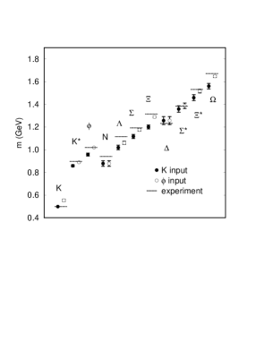
Figure 13: The spectrum of light mesons and baryons obtained in the quenched approximation after extrapolation to $u,d$ quark masses and to the continuum limit. The $\rho$ and $\pi$ masses are missing since they were used to fix the lattice spacing and $u,d$ masses. Results are compared using the $K$ or the $\phi$ to fix the strange quark mass and disagreement between the two is seen. The size of the discrepancy with experiment depends on this and varies between hadrons, but is at the level of 10%. (Aoki, 2000, CP-PACS collaboration)

The quenched approximation also does not allow the decay of particles where this requires the production of a $\overline{q}q$ pair from the vacuum, e.g $\rho\rightarrow\pi\pi$. Once dynamical quarks are light enough for this to happen, it will in fact be difficult to determine $m_{\rho}$ since we will obtain instead the lighter mass of the two-pion system. It is then important in dynamical simulations to use hadrons which are stable in QCD, or have very narrow widths, to fix the quark masses in the QCD action.

It has been stressed that the numerical cost of unquenched calculations is very high. It increases very rapidly as $a$ is reduced at fixed physical volume and as $m_{u,d}$ is reduced, although the exact scaling behaviour is not completely clear. Figure 14 estimates the cost of generating an ensemble of 500 gluon configurations on an $L^{3}\times T$ lattice with $L$ = 3fm and $T=2L$ at a lattice spacing, $a$ = 0.1fm, as a function of the $u,d$ dynamical quark mass. The $x$ axis is plotted as the ratio $m_{\pi}/m_{\rho}$ where the $\pi$ and $\rho$ are the pseudoscalar and vector mesons made with valence quarks of the same mass as the dynamical quarks. The real world has $m_{\pi}/m_{\rho}$ = 0.2. For $m_{u,d}=m_{s}$ the ratio is 0.7, for $m_{u,d}=m_{s}/2$, 0.55 and for $m_{s}/4$, 0.4. For $m_{s}/2$ the ratio is obtained from the $K$ and $K^{{\displaystyle*}}$ masses. For $m_{s}$ and $m_{s}/4$ some arguments must be made about the scaling of hadron masses with quark masses because, for example, no pure $s\overline{s}$ pseudoscalar meson exists. The cost varies here as $(m_{\pi}/m_{\rho})^{3}$, which is based on estimates from simulations (LAT2001). Figure 14 compares the cost for clover quarks and improved staggered quarks, again based on simulations at one quark mass, and using the same scaling formula. The cost advantage of improved staggered quarks is clear on this plot. One disadvantage is that the algorithm generally used for two flavors of dynamical staggered quarks is not exact, unlike that for clover. This means that there are systematic errors, rather like discretisation errors, which increase with the computer time step, $\epsilon$, which is used to generate one gluon configuration from the previous one. Checks must to be done to make sure that this systematic error is at an acceptable level and/or an extrapolation to $\epsilon$ = 0 must be done.

Figure 14: The computer cost in teraflop-years of generating 500 $30^{3}\times 60$ configurations with $a=$ 0.1fm and a dynamical quark mass which gives the ratio of pseudoscalar to vector meson masses along the $x$ axis. Clover and improved staggered quarks are compared, assuming the same scaling behaviour as $(m_{\pi}/m_{\rho})^{3}$. The straight line shows what is possible in 6 months on a 5Tflops computer.

Recent unquenched calculations, albeit with rather heavy dynamical quark masses, have shown encouraging signs that systematic errors from the quenched approximation are being overcome. Figure 12 shows that the ratio of $a^{-1}$ values obtained from two different quantities is closer to 1 on dynamical configurations (using two flavors of dynamical quarks with a mass around $m_{s}$) than it was on quenched configurations (Marcantonio, 2001, UKQCD collaboration). From this we can hope that with 2 dynamical light quarks and a dynamical strange quark there will be only one value of the lattice spacing, corresponding to the one dimensionful scale of QCD in the continuum.

Figure 15 compares results for the masses of $\phi$ and $K^{{{\displaystyle*}}}$ mesons on quenched and unquenched configurations as a function of $a$. The $K$ meson is used to fix $m_{s}$ and gives poor results for the $K^{{\displaystyle*}}$ and the $\phi$ in the quenched approximation, as described earlier. For two flavors of dynamical quarks, the $K^{{\displaystyle*}}$ and $\phi$ masses are much closer to experiment, at least after a continuum extrapolation (Ali Khan, 2002, CP-PACS collaboration). One worrying feature of this plot is the size of discretisation errors in the unquenched case, implying that the improved action used does not work as well in that case.

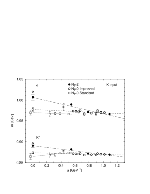
Figure 15: The masses of the $\phi$ and $K^{{\displaystyle*}}$ mesons as a function of lattice spacing, $a$, for quenched simulations and those using two flavors of dynamical quarks. The $K$ meson is used to fix the strange quark mass. The experimental results are indicated by diamonds at $a=$ 0. The Iwasaki improved gluon action was used with a clover quark action. (Ali Khan, 2002, CP-PACS collaboration)

Figure 16 shows another quantity from light hadron physics that gives a problem in the quenched approximation. This is the difference of the squared vector and pseudoscalar masses for given quark combinations. Experimentally the result is very flat as a function of quark mass, being $\approx 0.55{\rm GeV}^{2}$ from the $\pi,\rho$ to the $D,D^{{\displaystyle*}}$. In the quenched approximation this quantity has a pronounced downward slope as the quark mass is increased. Recent results from the MILC collaboration with 2 ($m_{s}/4$) + 1 ($m_{s}$) flavors of dynamical improved staggered quarks show qualitatively different behaviour, much closer to that of experiment (Bernard, 2001, MILC collaboration). This is the strongest indication yet that calculations with dynamical quarks will overcome the disagreements between the quenched approximation and experiment.

Figure 16: The difference of the squares of the vector and pseudoscalar masses for various light hadrons, obtained with quenched and dynamical lattice QCD. The dynamical results have 2+1 flavors of dynamical quarks with masses $\approx m_{s}/4$ and $m_{s}$. The dynamical results are given only for valence quark masses equal to the dynamical ones. Experimental results are given by the bursts, using an estimated mass for the pseudoscalar $s\overline{s}$ meson. The lattice spacing has been obtained using $r_{0}=0.5$fm. Errors do not include errors from fixing the lattice spacing (Bernard, 2001, MILC collaboration).

4 Lattice QCD results

The Proceedings of each year’s lattice conference provide a useful summary of current results and world averages. See (LAT2000, LAT2001). Almost all lattice papers can be found on the hep-lat archive, http://arXiv.org/hep-lat/. I have deliberately chosen to refer to reviews where possible and these should be consulted for fuller access to the literature.

4.1 Methods for heavy quarks

Bottom and charm quarks are known as heavy quarks since they have masses much greater than the typical QCD scale, $\Lambda_{\rm QCD}$, of a few hundred MeV. Top quarks are also heavy, of course, but do not have interesting bound states so are not studied by lattice QCD. $b$ and $c$ quarks could be treated in the same way as $u$, $d$, or $s$ quarks on the lattice except that, with current lattice spacings of about 0.1fm, we have $m_{b}a$ in the interval 2–3 and $m_{c}a$ in 0.5–1. If $ma$ is not small then discretisation errors of the form $ma$, $(ma)^{2}$ etc. will not be small either and such an approach will not give accurate results. Relativistic momenta, $\hbox{}{p}\approx m$, can also not be well simulated if $\hbox{}{p}a$ is not small: $\hbox{}{p}a$ of $O(1)$ corresponds to wavelengths which are in danger of being small enough to ‘fall through’ the holes in the lattices.

To reach the very fine lattices that would be required to give $m_{b}a\ll 1$ and accurate simulations for $b$ quarks would require an amount of computing power way beyond our current hardware even in the quenched approximation. Luckily the physics of heavy quark systems in the real world means that we do not have to do this; indeed, it would be largely a waste of computer power. $b$ and $c$ quarks are non-relativistic in their bound states, so that $m$ and $\hbox{}{p}\approx m$ are irrelevant dynamical scales. The non-relativistic nature is evident from the hadron spectrum. There are heavy-heavy bound states in which both the valence quark and anti-quark are heavy ($\Upsilon$, $\psi$ and $B_{c}$) and heavy-light bound states in which the heavy (anti-)quark is bound to a light partner ($B$, $B_{s}$, $D$, $D_{s}$) or partners, in the case of baryons ($\Lambda_{b}$, $\Lambda_{c}$). In all cases the mass difference (splitting) between excitations of these quark systems is much less than the mass of the hadrons. For example $m(\Upsilon^{\prime}){-}m(\Upsilon)=560$MeV, $m(\Upsilon)$ = 9.46GeV. The internal dynamics, which controls these splittings, operates with scales much smaller than the quark mass. Instead the important scales are the typical momentum carried by the quark inside the bound state, $mv$, and the typical kinetic energy, $\frac{1}{2}mv^{2}$. That these scales are small compared to $m$ implies that $v/c\ll 1$. The use of non-relativistic techniques on the lattice is then a good match to the physics of $b$ and $c$ systems as well as providing an efficient way to handle them numerically on the lattice.

There are several ways to proceed, and it is important when reading the lattice literature to understand which method has been used. In the remainder of this section we consider three methods in particular: (a) static quarks, (b) NRQCD (a non-relativistic version of QCD) and (c) heavy relativistic quarks.

Static quarks

This is the $m=\infty$ limit of heavy quarks. In this limit Heavy Quark Symmetry holds and quarks become static sources of colour charge with no spin or flavor. This is evident on the lattice as the quark propagator becomes simply a string of gluon fields along the time direction (Eichten, 1990). Obviously no real quarks have infinite mass but this is a useful limit for studying heavy-light systems. Corrections away from the infinite mass limit are the subject of Heavy Quark Effective Theory (Buchalla, 2002).

NRQCD

NRQCD is a non-relativistic version of QCD (Lepage, 1992). The Lagrangian for heavy quarks is the non-relativistic expansion of the Dirac Lagrangian:

$${\cal{L}}_{Q}=\overline{\psi}(D_{t}-\frac{\mathbf{D}^{2}}{2m_{Q}a}-c\frac{\bm{\sigma}{\cdot}\mathbf{B}}{2m_{Q}a}+\cdots)\psi$$ (34)

where additional terms can be added to go to higher order in $v/c$. $\psi$ is now a 2-component spinor since the quark and anti-quark fields of the Dirac fields decouple from each other. $D$ is a covariant derivative, including coupling to the gluon field. $\mathbf{B}$ is the chromomagnetic field, related to space-space components of the field strength tensor, $B_{i}=\epsilon_{ijk}F_{jk}$. $m_{Q}$ is the quark mass; heavy quarks are frequently generically denoted $Q$ in contrast to the $q$ used for light quarks. Notice that the quark mass term $\overline{\psi}m_{Q}a\psi$ has been dropped. This simply redefines the zero of energy so that the energies of all hadrons in lattice units are less than 1.

The NRQCD Lagrangian can be discretised onto a lattice and leads to much simpler and faster numerical algorithms for calculating the quark propagator than for light quarks. Instead of having to explicitly invert a matrix using an expensive iterative procedure such as Conjugate Gradient, the propagator is simply calculated by stepping through the lattice in time and calculating the propagator at time $t$ from that at time $t-1$. This is simply illustrated if we look at the Lagrangian in the infinite mass limit, where it becomes the Lagrangian for static quarks. Only the first term above contributes and we have:

$$S_{Q}=\sum_{x}\overline{\psi}(x)\left(\rule[-4.30554pt]{0.0pt}{12.91663pt}U_{t}(x)\psi(x+1_{t})-\psi(x)\right)$$ (35)

$M$ is then an upper triangular matrix, using the notation of Equation 27, and the quark propagator is given by:

$$(M^{-1,Q}_{0,t+1})=U^{{\dagger}}_{t}(M^{-1,Q}_{0,t}).$$ (36)

The general start and end points, $x$ and $y$, are simply denoted here by their $t$ co-ordinates, 0 for the origin and $t$ for the end point. To move from end point $t$ to $t+1$ just requires multiplication by the appropriate $U$ field in the time direction, so $M^{-1}$ does not change spatially and becomes a string of $U$ fields as described for static quarks above. For NRQCD with non-infinite masses, the evolution equation in $t$ for the propagator is not as simple and does contain spatial variations (e.g. from the spatial covariant derivatives in Equation 34) but the same principles apply. A smearing function, $\phi$, is chosen at the time origin and then the propagator calculated from 0 to later times by an evolution equation from one $t$ to the next. This makes NRQCD numerically very attractive. Heavy quark propagators, once calculated, can be combined together or with a light quark propagator to make 2- and 3-point functions for heavy hadrons as described for light hadrons earlier. As described there also, the value for the bare heavy quark mass in lattice units, $m_{Q}a$, is adjusted, given a value for $a$, until a heavy hadron mass is correct in GeV. The energies of heavy hadrons calculated on the lattice do not in fact equate directly to their masses because the mass term was removed from the Lagrangian. Instead, for one heavy hadron we have to calculate an energy-momentum dispersion relation and derive its mass from the momentum dependence ($E\propto\mathbf{p}^{\,2}/2M$).

NRQCD is an effective theory, containing the right physics for low momentum heavy quarks. Adding more relativistic corrections to the Lagrangian can make this more accurate. These higher order terms appear with coefficients (such as $c$ in equation 34) which must be determined by matching to relativistic QCD. These coefficients represent the effect of relativistic momenta missing from NRQCD and they are governed by $\alpha_{s}$ at this high momentum scale and so are perturbative. High momenta for both quarks and gluons are missing anyway on the lattice because of the discretisation of space-time. We described earlier how a better match between lattice QCD and QCD is made by adding terms to the lattice QCD Lagrangian which are higher order in $a$, with a coefficient which depends on the strong coupling constant at the lattice cut-off scale. That the two procedures are very similar is not an accident; indeed, the same higher dimension operators appear in both cases. In this case NRQCD is simply making a virtue of the existence of the lattice cut-off. The difference is, however, that in the NRQCD case the operators appear with inverse powers of $m_{Q}a$ (in a dimensionless lattice notation) and so $m_{Q}a$, and therefore $a$, cannot be taken to zero in this approach. NRQCD has no continuum limit, but this does not prevent physical results being obtained at finite lattice spacing. It is just necessary to show that the results are sufficiently independent of $a$ over a range of values of $a$.

Heavy relativistic quarks

This method looks very different from NRQCD, but has a lot of features in common. The use of a relativistic action, such as the Wilson/clover action, for heavy quarks on a lattice does not have to be incorrect if the results are interpreted carefully (El-Khadra, 1997). The main point to realise is that the existence of a large value for $ma$ breaks the symmetry between space and time. The inverse quark propagator in momentum space has an energy at zero momentum very different from its mass (e.g. for a free Wilson quark, $E(\mathbf{p}=0)=\ln(1+ma)$) but its momentum dependence for small momenta is correct (i.e. as $\mathbf{p}^{\,2}/ma$). Thus, we can ignore the $ma$ errors in the energy if we fix masses from the energy-momentum relation as for NRQCD. For more precision we must add higher order discretisation/relativistic corrections. These will appear with coefficients chosen to match continuum relativistic QCD. As we have seen the coefficients are a power series in $\alpha_{s}$ at the cut-off scale and they will depend on $ma$. For small $ma$ the coefficients will be those of a discretisation correction to the action; for large $ma$ they will go over to the NRQCD coefficients. For example, the $\sigma_{\mu\nu}F_{\mu\nu}$ clover term corrects for an ${O}$$(a)$ error in the Wilson action for light quarks; for heavy quarks, it becomes the relativistic correction which couples the quark spin and the chromomagnetic field. In this way an action can be developed that smoothly interpolates between heavy and light quark physics, at the numerical cost of having to handle heavy quarks in the same way as light ones. This method is sometimes known as the Fermilab method, since it was pioneered there.

The charm quark mass is not very heavy on the finest of current quenched lattices, and some groups have taken the standard relativistic approach in this case. To reach the $b$ quarks then requires an extrapolation jointly in the heavy quark mass and the lattice spacing (Maynard, 2002, UKQCD collaboration) to avoid confusing discretisation and relativistic corrections. Such an extrapolation inevitably has rather large errors. A better approach is to consider a formalism which explicitly breaks space-time symmetry in order to restore the relativistic energy-momentum relation for heavy quarks. For example, you can take an anisotropic lattice which has a much finer spacing in the time direction than in the space directions. $ma_{t}$ is then small and the heavy quark looks like a light one, at the cost of having many more timeslices on the lattice, and having to determine the lattice spacing in both directions (Chen, 2001).

4.2 The heavy hadron spectrum

The spectrum of heavy-heavy states has largely been the province of NRQCD (Davies, 1998). Figure 17(a) shows the radial and orbital excitations of the $b\overline{b}$ $\Upsilon$ system, obtained both on quenched gluon configurations and those with two flavors of dynamical quarks (Marcantonio, 2001, UKQCD collaboration). For these results the lattice spacing has been fixed by demanding that the splitting between the $\Upsilon(1S)$ and the spin-average of the $P$-wave ($\mbox{\raisebox{1.72218pt}{$\chi$}}_{b}$) states is correct. The $b$ quark mass has been fixed by requiring that the $\Upsilon(1S)$ mass be correct. It is only the $2S$ ($\Upsilon^{\prime}$), $3S$ ($\Upsilon^{\prime\prime}$) and $2P$ ($\mbox{\raisebox{1.72218pt}{$\chi$}}_{b}^{\prime}$) states that are predicted from this calculation, and they have rather large statistical errors at present. It is a general feature of lattice calculations that ground state masses are more precise than excited state masses. For both excited and ground states the noise is controlled by the ground state mass. For excited states the signal/noise ratio is then much worse and becomes exponentially bad at large $T$.

Of more immediate interest is the fine structure of the low-lying $S$ and $P$ states, shown in Figure 17(b). These can be determined very precisely on the lattice, particularly the ‘hyperfine’ splitting between the spin-parallel vector $\Upsilon$ state and the not-yet-seen spin-antiparallel pseudoscalar $\eta_{b}$. A comparison with experiment, when it exists, for this splitting will provide a very good test of lattice QCD and our $b$ quark action, which will be important for the lattice predictions of $B$ matrix elements described in Section 4.3.

 (a) (b)

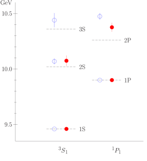
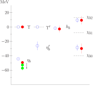
Figure 17: (a) The radial and orbital excitations in the $b\overline{b}$ system, as calculated in lattice QCD using NRQCD for the $b$ quarks (Marcantonio, 2001, UKQCD collaboration). (b) The fine structure of low-lying $b\overline{b}$ states. Legend: the horizontal dashed lines are experimental values; open circles show the quenched approximation; solid circles correspond to 2 flavors of clover dynamical quarks with mass $m_{s}$. (The lowest cluster of points on the right show an extrapolation to lighter dynamical mass and to $N_{f}{=}3$.)

The accuracy of the NRQCD, or other lattice action, for heavy-heavy bound states can be estimated by working out what order in an expansion in powers of $v/c$ is represented by each term. e.g. the first two terms in the NRQCD action of Equation 34, i.e. the time derivative and the kinetic energy term, are both ${O}$$(v^{2}/c^{2})$. This is because the ‘potential energy’ and kinetic energy terms are roughly equal for two heavy particles. These terms give rise to the radial and orbital splittings, and the ratio of these ($\approx$ 500MeV) to half the $\Upsilon$ mass gives an estimate of $v^{2}/c^{2}\approx 0.1$ for $b$ quarks in an $\Upsilon$. Higher relativistic corrections, such as the $\mathbf{D}^{4}/8m_{Q}^{3}$ term, are ${O}$$(v^{4}/c^{4})$ and should give roughly a 10% correction to these splittings. These terms were included here, but not the $v^{6}/c^{6}$ corrections, so an error of roughly 1% remains. The $\bm{\sigma}\cdot\mathbf{B}$ term of Equation 34 is the first spin-dependent term and is ${O}$$(v^{4}/c^{4})$. It gives rise to the hyperfine splitting and a similar term of the same order, proportional to $\bm{\sigma}\cdot\mathbf{D}\times\mathbf{E}$, gives rise to the $P$ fine structure. The fine structure is indeed roughly 10% of the radial and orbital splittings. Including only these terms in the NRQCD action, as was done here, implies an error of roughly 10% in these splittings. A more precise calculation, necessary to test this action against experiment, will require the $v^{6}/c^{6}$ spin-dependent terms and the $\alpha_{s}v^{4}/c^{4}$ terms implied by calculating the coefficient $c$ in front of the $\bm{\sigma}\cdot\mathbf{B}$ term in equation 34. This is now being done. Figure 17(b) does show, however, that the hyperfine splitting increases when two flavors of dynamical quarks are included, and continues to increase as the dynamical quark mass is reduced towards real $u$ and $d$ quark masses. We expect the $\Upsilon$ to see also $s$ quarks in the vacuum and extrapolating the number of dynamical flavors to three increases the splitting further.

The charmonium, $\psi$, system is more relativistic that the $\Upsilon$ system and correspondingly less well-suited to NRQCD. Estimates as above give $v^{2}/c^{2}\approx 0.3$. Figure 18 shows the charmonium spectrum obtained from anisotropic relativistic clover quarks in the quenched approximation (Chen, 2001). The lattice spacing and charm quark mass were fixed in the analogous way to that described above, except that the spin average of the vector $J\psi$ and pseudoscalar $\eta_{c}$ masses was used to fix $m_{c}$. Since the $\eta_{c}$ mass is known experimentally this gives improved precision since the spin-average is not sensitive to any inaccuracies in spin-dependent terms. The spectrum given in Figure 18 includes some gluonic excitations of the $c\overline{c}$ system, i.e. $c\overline{c}g$ states, called hybrids. Their existence is expected simply from the non-Abelian nature of QCD which allows gluons themselves to carry color charge. Some of these hadrons have exotic quantum numbers not available to mesons made purely of valence quarks, and the prediction of their masses will be important for their experimental discovery.

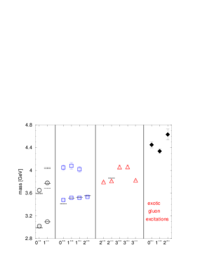
Figure 18: The spectrum of $c\overline{c}$ states, as calculated in lattice QCD using anisotropic quenched configurations (Chen, 2001).

Figure 19 shows the spectrum of mesons made from one $b$ quark and one light ($u/d$ or $s$) anti-quark in the quenched approximation (Hein, 2000). NRQCD was used for the $b$ quark, and the clover action for the light quark. In this case the lattice spacing was fixed using a quantity from the light hadron spectrum, $m_{\rho}$, because heavy-light systems are more similar in terms of internal momentum scales to light hadrons than heavy-heavy ones. See the comments in Section 3.2 on how the lattice spacing in the quenched approximation depends on the quantity used to fix it. The $u/d$ and $s$ quark masses were fixed using the $\pi$ and $K$ masses. The $b$ quark mass was fixed from the spin-average of the $B$ and $B^{{\displaystyle*}}$ meson masses. Taking a spin-average, as above for charmonium, avoids any errors from spin-dependent terms in the action. The $b$ quark mass obtained this way differs from that obtained above from the $\Upsilon$ system, and is another feature of the quenched approximation. In the ‘real world’ there is only one lattice spacing and one set of quark masses and parameters fixed from the $\Upsilon$ system will be used to predict the entire $B$ spectrum.

Figure 19: The spectrum of bound states of a $b$ quark with a light anti-quark as calculated in lattice QCD in the quenched approximation using NRQCD for the $b$ quark (Hein, 2000).

The power counting in $v/c$ for terms in the Lagrangian works rather differently in heavy-light systems compared to heavy-heavy ones. Now there is one quark that carries almost all the mass of the heavy-light system and it sits in the centre surrounded by the swirling light quark cloud. This picture makes sense even in the limit in which the heavy quark has infinite mass when the Lagrangian would contain only the covariant temporal derivative $D_{t}$ (static quarks). The higher order terms in the Lagrangian can then be ordered in terms of the inverse powers of the heavy quark mass that they contain. This is equivalent to an expansion in powers of $v/c$. The typical momentum of a heavy quark in a heavy-light system is ${O}$$(\Lambda_{\rm QCD})$ (as is that of the light quark) and so $v/c\approx\Lambda_{\rm QCD}/m_{Q}$. This gives $v/c\approx$ 10% for the $B$ and 30% for the $D$.

Again the power counting exercise enables us to understand the approximate relative sizes of different mass splittings in the spectrum and the accuracy of our lattice QCD calculation to a given order in $v/c$. The leading spin-independent term in the action is $D_{t}$ giving rise to the orbital and radial excitations of $\approx$ 500MeV. The kinetic energy term, $\mathbf{D}^{2}/2m_{Q}$ gives a $\Lambda_{\rm QCD}/m_{Q}$ correction to this, which depends on the quark mass and, therefore flavor. This explains why these excitation energies are so similar for $B$ and $D$ systems; the similarity between $\psi$ and $\Upsilon$ is more accidental. The leading spin-dependent term is $\bm{\sigma}{\cdot}\mathbf{B}/2m_{Q}$, which gives rise to fine structure such as the splitting between the pseudoscalar $B$ and vector $B^{{\displaystyle*}}$. This splitting should then be smaller by a factor of $\Lambda_{\rm QCD}/m_{Q}$ compared to the spin-independent splittings and this is indeed observed. To calculate this splitting precisely on the lattice requires the inclusion of higher order terms in the Lagrangian, as well as a better matched coefficient $c$ for the $\bm{\sigma}\cdot\mathbf{B}$ term and this will be done in future calculations.

We have stressed that lattice QCD is simply a way of handling QCD. It has the same a priori unknown parameters as QCD, the overall scale (equivalent to the coupling constant) and the quark masses. These parameters come from a deeper theory and must simply be fixed in the QCD Lagrangian using experiment and the results from a calculation in QCD. As described in Section 3, Lattice QCD provides the most direct way of doing this. The values for the parameters obtained are then useful input to other theoretical techniques.

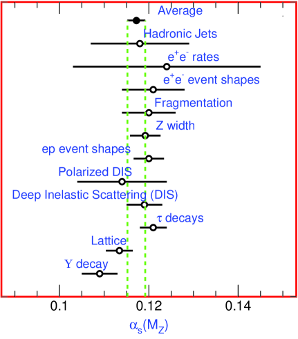
Figure 20: A comparison of determinations of the strong coupling constant, expressed as $\alpha_{s}^{\overline{MS}}(M_{Z})$ (PDG, 2001).

Determination of the lattice spacing at a given lattice bare coupling constant, is equivalent to (and can be converted into) a determination of the renormalised coupling constant, $\alpha_{s}$, at a physical scale in GeV. To compare to other determinations of $\alpha_{s}$, this can be converted to the $\overline{MS}$ scheme and run to $M_{Z}$. Figure 20 shows a comparison of different determinations of $\alpha_{s}$ from the Particle Data Group (PDG, 2001). It is clear that the lattice result is one of the most precise.

All methods for determining $\alpha_{s}$ have three components:

1. Theoretical input: a perturbative expansion in $\alpha_{s}$, for some quantity.

2. A value for that quantity.

3. An energy scale.

Most methods use an experimental result for stage 2, where the lattice uses a non-perturbative evaluation on the lattice of the vacuum expectation value of a simple short-distance gluonic operator (such as the plaquette). This avoids the problems of hadronisation etc which reduce the precision of methods based on the experimental determination of jet shapes or cross-sections. All methods use experiment for stage 3, and here the lattice-based determination needs an experimental result to fix the lattice spacing. A good quantity to use here is the orbital excitation energy ($1P{-}1S$) in, say, the $\Upsilon$ system since this is well-determined on the lattice and directly measured experimentally.

Quark masses are also well determined on the lattice. Since quarks are not freely available to be weighed, as an electron would be, care must be taken in defining what exactly is meant by the quark mass. The bare mass in the lattice QCD Lagrangian for a particular action, determined by the requirement to get a particular hadron mass correct and converted to physical units, is a well-defined quantity but not very convenient. We can convert it perturbatively into, say, the running quark mass in the $\overline{MS}$ scheme. The best current determination of the $b$ quark mass is in fact from the static approximation in which $b$ quarks have infinite mass. There is no bare $b$ quark mass in that case; instead the binding energy $m_{B}-m_{b}$ is calculated, and from that, $m_{b}$ is determined. The binding energy is small compared to $m_{B}$ and has only weak dependence on the $b$ quark mass, so for this quantity the static approximation is a good one. The $b$ quark mass obtained in this way is 4.30(10)GeV in the quenched approximation, with some indications that it is slightly lighter when dynamical quarks are included (Lubicz, 2001).

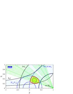
Figure 21: The unitarity triangle with constraints on the upper vertex obtained from different quantities (Hocker, 2001). The lower vertices are at $\overline{\eta}$ = 0, $\overline{\rho}$ = 0 and 1.

4.3 Heavy hadron matrix elements

Precise lattice calculations of matrix elements for $B$ decay are essential to the experimental $B$ factory programme (Stone, 2002). This aims to test the internal consistency of the Standard Model in which CP violation occurs through the Cabibbi-Kobayashi-Maskawa matrix. The weak decays of the $b$ quark are particularly useful in giving us access to poorly known elements of this matrix. The unitarity of the CKM matrix can be represented by a triangle; the position of the upper vertex being constrained by the determination of angles and sides, see Figure 21. The angles are determined directly by measurement of asymmetries. The determination of the sides requires both the experimental measurement of a decay rate and its theoretical calculation.This allows the magnitude of one of the CKM elements to be extracted. Below we describe the lattice calculation of the matrix elements most important for this programme. The extent to which the unitarity triangle can be tested depends on both the experimental and the theoretical errors. It is critical to reduce the errors from lattice calculations to a few percent, otherwise they will dominate the uncertainties from experiment.

The simplest 2-point matrix element that can be calculated on the lattice is that for the decay constant of the charged pseudoscalar heavy-light mesons (see Figure 8). For the $B$ this is known as $f_{B}$ and it is obtained from the vacuum to $B$ matrix element of the axial vector current which couples to the $W$.

$$\langle 0|A_{\mu}|B\rangle=p_{\mu}f_{B}.$$ (37)

The purely leptonic decay rate of the $B$ meson is then proportional to $f_{B}^{2}$ times kinematic factors times the square of the CKM element which multiplies the appropriate axial vector current in the Lagrangian, in this case $\overline{u}\gamma_{\mu}\gamma_{5}b$ (Rosner, 2002). In principle an experimental determination of the leptonic decay rate could be combined with the lattice calculation to yield $V_{ub}$, but in practice the experiment is very hard to do because the rate is so low. For other heavy-light mesons, it may be possible. $f_{D_{s}}$ has been measured experimentally, but not very precisely as yet. It can be used, with lattice calculations, to give $V_{cs}$.

It is important to realise that, although we are discussing the weak decay of a $b$ or $c$ quark, the calculations are done in lattice QCD. The quark cannot decay in isolation, but must be bound into a hadron by the confinement property of QCD. The determination of the decay matrix element must then take into account all the QCD interactions inside the hadron (see Figure 8) and this requires lattice QCD. We do not put the $W$ boson on the lattice. As far as QCD is concerned the $B$ meson annihilates into the vacuum. The virtual $W$ boson decay to leptons is put in by hand when we calculate the decay rate.

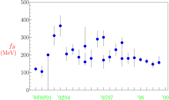
Figure 22: A timeline of results for the $B$ meson decay constant, $f_{B}$, calculated in lattice QCD in the quenched approximation.

Lattice calculations of $f_{B}$ improved markedly through the 1990s (this has been true of most lattice calculations) as we got to grips with the systematic errors. Figure 22 shows a timeline of results in the quenched approximation. It shows both that lattice calculations have markedly improved and that early calculations had very unreliable estimates of their errors. The most recent and best calculations do a careful job of matching the lattice representation of the axial vector current to the continuum. For heavy-light mesons we have to be careful both about relativistic ($\Lambda_{\rm QCD}/m_{Q}$) corrections and discretisation corrections to the leading order lattice current. Since $m_{Q}a$ is a dimensionless number, these two corrections in fact appear together and can be considered simultaneously. The matching between lattice and continuum is currently done only to ${O}$$(\alpha_{s})$ and this is the major source of error in the quenched approximation. Table 1 shows a typical ‘error budget’ for such a calculation. We need a more precise matching, either to $\alpha_{s}^{2}$ or non-perturbatively (both of which can be done with a lot of hard work), to improve the errors beyond the 10% level.

Source	percent error
statistical + fitting	$3$
discretisation $O((a\Lambda)^{2})$	4
perturbative $O(\alpha_{s}^{2},\alpha_{s}^{2}/(aM))$	7
NRQCD $O((\Lambda/M)^{2},\alpha_{s}\Lambda/M)$	2
light quark mass	4
$a^{-1}(m_{\rho})$	4
Total	10

Table 1: Source of error in a typical lattice calculation of $f_{B}$ using NRQCD for the heavy quark in the quenched approximation. $a\approx 0.1$fm, $M$ is the $b$ quark mass, $\Lambda$ a typical QCD scale of a few hundred MeV and $\alpha_{s}$ is evaluated at $2/a$.

Recent reviews of lattice results (Ryan, 2002), (Bernard, 2001) have given the following ‘world averages’ for lattice results in the quenched approximation:

• $f_{B}$ = $173\pm 23$MeV

• $f_{D_{s}}$ = $230\pm 14$MeV

• $f_{B_{s}}/f_{B}$ = 1.15(3); $f_{D_{s}}/f_{D}$ = 1.12(2).

(Note that the $B_{s}$ does not decay purely leptonically but the calculation of the appropriate matrix element can still be done in lattice QCD and yields useful information on its dependence on the light quark mass.) Large-scale calculations on dynamical configurations are only just beginning, so unquenched results are still unclear. It seems likely that decay constants will be 10–20% larger unquenched.

A more important quantity from the point of view of the $B$ factory programme is the mixing amplitude for neutral $B$ mesons, $B^{0}$ and $B_{s}$. This mixing gives rise to a difference in mass between the CP-eigenstates, $\Delta m$, which can be measured experimentally through oscillations between particle and anti-particle (Stone, 2002). The mixing amplitude is given by the ‘box diagram’ (see Figure 23) in which the $b$ quark and light anti-quark convert to a $b$ anti-quark and light quark through the mediation of virtual $W$s and (preferentially) $t$ quarks. The mixing amplitude is then proportional to the matrix element of the box between, say, a $B^{0}$ and a $\overline{B}^{0}$ multiplied by the product of CKM elements $V_{tb}^{{\displaystyle*}}V_{td}$. The current determination of $|V_{td}|^{2}$ from experiment and theory gives a curve on the unitarity triangle plot (marked $\Delta m_{d}$ on Figure 21). Future experiments will be able to see oscillations of the $B_{s}$ and then ratios of $\Delta m_{B_{s}}/\Delta m_{B}$ will allow a more precise determination of $|V_{ts}/V_{td}|^{2}$, since some of the systematic errors will cancel out.

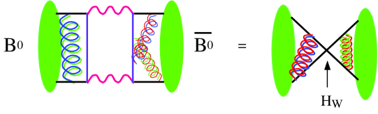
Figure 23: The $B$ box diagram, related to that of a 4-quark operator.

As explained earlier, $W$ bosons do not appear in lattice QCD calculations. The matrix element of the box diagram is calculated in lattice QCD by replacing it with the equivalent 4-quark operator which appears in the effective (low-energy) weak Hamiltonian (Rosner, 2002). Conventionally this matrix element for the $B$ is set equal to $(8/3)f_{B}^{2}M_{B}^{2}B_{B}$, giving a definition of the parameter confusingly called $B_{B}$. $B_{B}$ is the amount by which the matrix element differs from the result that would be obtained by saturating the $H_{W}$ vertex of Figure 23 with the vacuum (comparing this to the right hand picture of Figure 8 we can see that this would be $f_{B}^{2}$). $B_{B}$ is generally expected to be roughly 1, and this explains why lattice calculations originally concentrated on calculating $f_{B}$. To calculate $B_{B}$ is harder, but is now being done. It requires, as for $f_{B}$, a careful matching between the lattice and the continuum, and this has again been done to ${O}$$(\alpha_{s})$ so far.

Recent world averages for the renormalisation-group-invariant definition of $B_{B}$ in the quenched approximation have been given as (Ryan, 2002), (Bernard, 2001):

• $\hat{B}_{B_{d}}$ = 1.30(12)(13)

• $f_{B_{d}}\sqrt{\hat{B}_{B_{d}}}$ =230(40)MeV

• $\hat{B}_{B_{s}}/\hat{B}_{B_{d}}$ = 1.00(4)

• $f_{B_{s}}\sqrt{\hat{B}_{B_{s}}}/f_{B_{d}}\sqrt{\hat{B}_{B_{d}}}$ = 1.15(6)

A lot of the matching errors cancel out in the ratios between $B_{s}$ and $B_{d}$ so that the errors in these ratios are less than 10%. The ratio may also not be significantly affected by unquenching.

Heavy-light mesons decay semi-leptonically through a diagram in which the heavy quark changes flavor, emitting a virtual $W$, and the other (spectator) quark in the meson combines with the new quark flavor to make a new meson. In this way $B$ mesons can decay to $D$ or $D^{{\displaystyle*}}$ mesons if $b\rightarrow c$ and to $\pi$ or $\rho$ mesons if $b\rightarrow u$. In each case the appropriate CKM element appears at the current vertex in the three-point diagram (see Figure 9) and can therefore be determined by a comparison of the experimental exclusive rate to the theoretical one. The ratio $V_{ub}/V_{cb}$ gives an important circular constraint in the unitarity triangle (see Figure 21).

The calculation of the matrix element for $B$ semi-leptonic decay on the lattice requires the calculation and simultaneous fitting of the 3-point function of Figure 9 and the appropriate 2-point functions necessary to isolate the matrix element. It is therefore significantly harder than a simple 2-point calculation. In addition the matrix element depends on $q^{2}$, the squared difference of 4-momenta between the initial and final meson. This can take a range of values, because the decay is a three-body one. The matrix element can then be written as a combination of form-factors which are $q^{2}$ dependent, in contrast to the two-body leptonic decay which was parameterised by a single number, $f_{B}$. For example the pseudoscalar to pseudoscalar transition (e.g. $B$ to $D$ or $\pi$) proceeds only through the vector current and has two form factors, $f_{+}$ and $f_{0}$:

$$\langle P^{\prime}(p^{\prime})|V_{\mu}|P(p)\rangle=f_{+}(q^{2})\left[(p+p^{\prime})_{\mu}-\frac{M_{P}^{2}-M_{P^{\prime}}^{2}}{q^{2}}q_{\mu}\right]+f_{0}(q^{2})\frac{M_{P}^{2}-M_{P^{\prime}}^{2}}{q^{2}}q_{\mu}$$ (38)

The differential decay rate is proportional to the square of $f_{+}$ because the leptonic current $L_{\mu}$ coupling to the $W$ has $q^{\mu}L_{\mu}=0$ for massless leptons. The pseudoscalar to vector transition proceeds through both the vector and axial currents and has 5 form factors, 3 of which appear in the decay rate.

To explore different values of $q^{2}$ for semi-leptonic decay on the lattice it is easiest to insert different 3-momenta at the final meson and at the current, and then work out the resulting 3-momentum of the initial meson. We are restricted to values of 3-momentum allowed on the lattice, i.e. the components of $\mathbf{p}$ have the form $p_{j}a=n_{j}2\pi/L$, where $n_{j}=0,1,2\ldots$ and $L$ is the number of lattice sites in the $j$ direction. The smallest non-zero value of $p_{j}$ is then $2\pi/(La)$ where $La$ is the physical size of the lattice in a spatial direction. A big physical volume is then required to achieve a fine discretisation of momentum space and avoid a large jump from one momentum to the next. In general results at higher momenta are much noisier than those at small momenta (this is for the same reason that excited states are noisier than ground states, discussed above) and calculations tend to be restricted to a few of the smallest possible momenta. Discretisation errors will also be larger at larger values of $pa$, so systematic errors will be higher.

For the matrix element for $B$ to $D^{({{\displaystyle*}})}$ semi-leptonic decay it is useful to consider both the $b$ quark and the $c$ quark in the heavy quark limit. In that limit, as discussed above, the Lagrangian for heavy quarks becomes insensitive to the heavy quark spin or flavour (Buchalla, 2002). The light quark cloud in the meson cannot tell whether it is surrounding a $b$ or a $c$ quark or one whose spin is pointing parallel or anti-parallel to its spin. Thus the form factors for $B\rightarrow D$ and $B\rightarrow D^{{\displaystyle*}}$ will become identical (or vanish) and the same as the $B\rightarrow B$ elastic form factor, provided they are viewed as a function of the right variable. This is not $q^{2}$ but $v{\cdot}v^{\prime}$ where $v$ is the 4-velocity ($p_{\mu}/m$) of the initial meson and $v^{\prime}$ is the 4-velocity of the final meson. $v{\cdot}v^{\prime}$ is often given the symbol $w$. In the notation of Equation 38 $w=(M_{P}^{2}+M_{P^{\prime}}^{2}-q^{2})/(2M_{P}M_{P^{\prime}})$. The limit $w=1$ is known as the ‘zero-recoil’ limit because this corresponds to the kinematic point where the $B$ meson at rest decays to, say, a $D$ meson at rest and the decay products of the $W$ come out back-to-back. This point has maximum $q^{2}=(M_{P}-M_{P^{\prime}})^{2}$.

The $B\rightarrow B$ elastic form factor takes the form

$$\langle B(v^{\prime})|V_{\mu}|B(v)\rangle=M_{B}\xi(w)(v+v^{\prime})$$ (39)

in the limit of infinite $b$ quark mass, where $\xi(w)=f_{+}(q^{2})$, $f_{-}=0$. $\xi(w)$ is known as the Isgur-Wise function. $\xi(1)=1$ is an absolute normalisation in the continuum because $\overline{b}\gamma_{\mu}b$ is a conserved current. The lattice current is not a conserved one (except for the NRQCD/static actions) but if we are interested only in the shape of $\xi(w)$ we can renormalise to match 1 at $w=1$. There have been several calculations of the $B\rightarrow B$ form factor on the lattice, for various heavy quark masses. Figure 24 shows such a calculation using NRQCD with a mass close to that for the $b$ quark (Hashimoto, 1996).

Figure 24: The $B\rightarrow B$ elastic form factor calculated in lattice QCD using NRQCD for the $b$ quark and plotted versus $w$ (Hashimoto, 1996).

The interest in calculating the Isgur-Wise function is that, in the Heavy Quark Symmetry picture described above, it is also applicable to $B\rightarrow D$ and $B\rightarrow D^{{\displaystyle*}}$ decays. In these cases, however, there is an additional overall perturbative renormalisation because $\overline{b}\gamma_{\mu}c$ is not a conserved current, and there are corrections which appear as differences of inverse powers of the $b$ and $c$ quark masses. For kinematic reasons, $B\rightarrow D^{{\displaystyle*}}$ is experimentally easier to measure in the $w\rightarrow 1$ region. The differential decay rate is

$$\frac{d\Gamma}{dw}=|V_{cb}|^{2}K(w){\cal F}^{2}(w)$$ (40)

where $V_{cb}$ is the CKM element that we want to determine, $K(w)$ is a kinematic factor and ${\cal F}$ is the form factor for the decay. Figure 25 shows results from the CLEO collaboration (CLEO, 2000) for ${\cal F}$$(w)|V_{cb}|$. The lighter hashed curve is the result from the lattice shown in Figure 24 rescaled by a constant to match at $w=1$. Given lattice results for $B\rightarrow D^{{{\displaystyle*}}}$ rather than $B\rightarrow B$, the constant required for rescaling would be $|V_{cb}|$ which would then be determined.

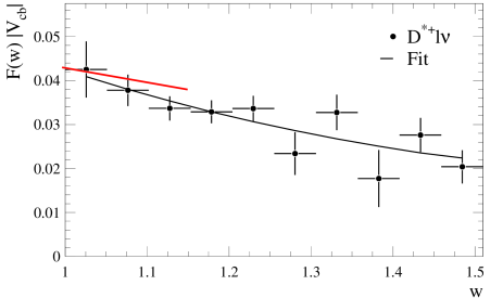
Figure 25: $|V_{cb}|F(w)$ extracted from the experimental $B\rightarrow D^{{\displaystyle*}}$ decay rate plotted as a function of $w$ (CLEO, 2000). The shorter curve on $1{<}w{<}1.15$ is a rescaled version of the curve in Figure 24.

In fact, a number of simplifications can be made to the lattice calculation at the $w=1$ point and so it is currently better to perform a phenomenological extrapolation of the experimental data to $w=1$ and divide the extrapolated result by the lattice result for $\cal F$$(1)$. The Fermilab group, using heavy relativistic (Fermilab) quarks and ${O}$$(\alpha_{s})$ matching to the continuum, give the most precise result so far:

$${\cal F}_{B\rightarrow D^{{\displaystyle*}}}(1)=0.913{}^{+0.024}_{-0.017}{}^{+0.017}_{-0.030}$$ (41)

in which the first error comes from statistics and fitting and the second from systematic errors, including the effect of using the quenched approximation (Hashimoto, 2001). The resulting value of $|V_{cb}|$ extracted depends on which experiment’s value for $|V_{cb}|{\cal F}(1)$ is taken. Using an average result (Stone, 2002) of $37.8\pm 1.4\times 10^{-3}$ gives a value for $V_{cb}$ of $41.4\pm 1.5\pm 1.7\times 10^{-3}$ where the final theoretical error comes from adding the lattice errors in quadrature. The lattice and experimental errors are currently of about the same size. The lattice error can be improved further in an unquenched calculation with a higher order matching of the lattice current to the continuum.

$B\rightarrow$ light ($\pi,\rho$) semi-leptonic decay is rather harder to calculate on the lattice. In many ways it is more important to do, however, because continuum techniques, such as HQET, can give very little useful input. One difficulty is that lattice systematic errors are smallest where the $B$ and, say, the $\pi$ lattice momenta are smallest, around the zero-recoil point discussed above, but there is very little experimental data there. Most experimental data occurs at relatively low $q^{2}$ values ($q^{2}<16{\rm GeV}^{2}$) when the zero recoil point has $q^{2}=q^{2}_{\rm max}=(m_{B}-m_{\pi})^{2}$ = 26${\rm GeV}^{2}$. A comparison of lattice results for the form factors for $B\rightarrow\pi$ decay is shown in Figure 26 (Bernard, 2001). Different lattice results are shown covering a range of $q^{2}$. The reason that some results are at smaller $q^{2}$ than others is because some use relativistic quarks (marked NPclover) at a mass around the $c$ quark mass rather than the $b$. For reasons discussed earlier, none of the lattice calculations can be done at the physical $u,d$ quark masses and so must be chirally extrapolated to that point. This is done in a different way by different groups and has led to very different final results, even though the intermediate data does not show very different behaviour (see Figure 26). A better understanding of how the chiral extrapolation should be done will be required before precise lattice results will be available. Good experimental results in the $q^{2}$ region that the lattice can reach will then allow a determination of $V_{ub}$.

 

Figure 26: Lattice results for the form factors for $B{\rightarrow}\pi$ decay (Bernard, 2001).

5 Conclusions

Lattice QCD has come a long way from the original calculations of the 1970s. The original idea that we could solve a simple discretisation of QCD numerically by ‘brute force’ has been replaced by a more sophisticated approach. Unfortunately, to the uninitiated, this can look like cookery. I have tried to describe some of the calculational and technical details so that non-practitioners feel able to make an informed judgement about lattice calculations, and see where progress will be made in the future. There is no doubt, for example, that precise lattice calculations are needed to obtain maximum benefit from the huge experimental investment in $B$ physics. In the next few years such calculations will become possible, at least for some quantities, and this will mark the ‘coming of age’ of the lattice QCD approach at last.

Acknowledgments

It was a pleasure to contribute to this lively and interesting school. I am grateful to all my collaborators, and particularly Peter Lepage and Junko Shigemitsu, for numerous useful discussions over many years. I am also grateful to Jack Cheyne, Greig Cowan and Alan Gray for a critical reading of this manuscript.

References

Ali Khan A et al, 2002, CP-PACS collaboration, Light hadron spectroscopy with two flavors of dynamical quarks on the lattice, Phys. Rev. D65 054505, hep-lat/0105015.

Aoki S et al, 2000, CP-PACS collaboration, Quenched light hadron spectrum, Phys. Rev. Lett. 84, 238; hep-lat/9904012.

Bernard C, 2001, Heavy quark physics on the lattice, Nucl. Phys. B (Proc. Suppl. 94) 159; hep-lat/0011064

Bernard C et al, 2001, MILC collaboration, The QCD spectrum with three quark flavors, Phys. Rev. D64 054506; hep-lat/0104002.

Buchalla G, 2002, Heavy quark theory, this volume; hep-ph/0202106.

Chen P, Liao X and Manke T, 2001, Relativistic quarkonia from anisotropic lattices, Nucl. Phys. B (Proc. Suppl. 94) 342; hep-lat/0010069.

CLEO collaboration, 2000, Determination of the $B\rightarrow D^{*}l\nu$ decay width and $|V_{cb}|$, hep-ex/ 0007052.

Davies C, 1998, The heavy hadron spectrum in Computing Particle Properties, Springer LectureNotes in Physics, Eds Gausterer, Lang; hep-ph/9710394.

Di Pierro M, 2001, From Monte Carlo Integration to Lattice Quantum Chromodynamics, hep-lat/0009001

Eichten E and Hill B, An effective field theory for the calculation of matrix elements involving heavy quarks, Phys. Lett. B243, 511.

El-Khadra A, Kronfeld A and Mackenzie P, 1997, Massive fermions in lattice gauge theory, Phys. Rev. D55, 3933; hep-lat/9604004.

Gupta R, 1998, Introduction to Lattice QCD, hep-lat/9807028.

Hashimoto S and Matsufuru H, 1996, Lattice heavy quark effective theory and the Isgur-Wise function, Phys. Rev D54 4578; hep-lat/9511027.

Hashimoto S et al, 2001, Lattice calculation of the zero-recoil form factor of $B\rightarrow D^{*}l\nu$: towards a model independent determination of $|V_{cb}|$, hep-lat/0110253.

Hein J et al, 2000, Scaling of the $B$ and $D$ meson spectrum in lattice QCD, Phys. Rev. D62 074503; hep-ph/0003130.

Hocker A, 2001, A new approach to gloabl fit of the CKM matrix, Eur. J. Phys. C21 25; hep-ph/0104062; http://www.slac.stanford.edu/~laplace/ckmfitter.html.

LAT2000, Nucl. Phys. B (Proc. Suppl. 94) 2001.

LAT2001, Nucl. Phys. B (Proc. Suppl. 106) 2002.

Lepage P and Mackenzie P, 1993, On the viability of lattice perturbation theory, Phys. Rev. D48, 2250; hep-lat/9209022.

Lepage P et al, 1992, Improved nonrelativistic QCD for heavy quark physics, Phys. Rev. D46, 4052; hep-lat/9205007.

Maynard C et al, 2002, UKQCD collaboration, Heavy-light decay constants on the lattice, Nucl. Phys. B (Proc. Suppl. 106), 388; hep-lat/0109026.

Lubicz V, 2001, Quark masses on the lattice, light and heavy, Nucl. Phys. B (Proc. Suppl. 94) 116; hep-lat/0012003.

Marcantonio L et al, 2001, UKQCD collaboration, The unquenched $\Upsilon$ spectrum, Nucl. Phys. B (Proc. Suppl. 94), 363; hep-lat/0011053.

PDG, 2001, http://pdg.lbl.gov/.

Rosner J, 2002, The Standard Model in 2001, this volume; hep-ph/0108195.

Ryan S, 2002, Heavy quark physics from lattice QCD, Nucl. Phys. B (Proc. Suppl. 106) 86; hep-lat/0111010.

Sommer R, 1998, Non-perturbative renormalisation of QCD in Computing Particle Properties, Springer Lecture Notes in Physics, Eds Gausterer, Lang; hep-ph/9711243.

Stone S, 2002, B Phenomenology, this volume; hep-ph/0112008.

Toussaint D, 2002, Spectrum results with Kogut-Susskind quarks, Nucl. Phys. B (Proc. Suppl. 106) 111; hep-lat/0110010.