TPJU-10/2002

PION GENERALIZED PARTON DISTRIBUTIONS
IN THE NON-LOCAL NJL MODEL

We calculate skewed parton distributions $H^{I}$ of a pion within a non-local NJL model with momentum dependent constituent quark mass $M(k)$. In the forward limit $H^{I}$ correspond to parton distributions, whereas for $t<0$ $H^{I}$ is related to the pion electromagnetic form-factor

1 Pion in the-non local effective theory

Pion being a Goldstone boson of the broken chiral symmetry and a $q\bar{q}$ bound state at same time has a unique status among strongly interacting particles. Experiments that measure pion generalized parton amplitudes (GDA) are therefore a direct tool to investigate the dynamics of the chiral symmetry breaking. Yet, compared to the nucleon, the experimental knowledge here is very limited. The most precise are measurements of the pion form-factor at low momentum transfer $\!{}^{{\bf?}}$. There exist also data on deep inelastic pion structure function $\!{}^{{\bf?}}$ measured in a Drell-Yan process and prompt photon production. Both are related to the pion skewed distribution $\!{}^{{\bf?}}$, $H^{I}$, at low normalization scale. To calculate $H^{I}$ we use the non-local chiral NJL model which follows from the instanton model of the QCD vacuum $\!{}^{{\bf?}}$. Here the external pion field

$$U^{\gamma_{5}}(x)=1+\frac{i}{F_{\pi}}\gamma^{5}\tau^{A}\pi^{A}-\frac{1}{2F_{\pi}^{2}}\pi^{A}\pi^{A}+\ldots$$ (1)

interacts with the constituent quarks

$$S_{I}=M\int\frac{d^{4}k}{(2\pi)^{4}}\bar{\psi}(k)F(k)U^{\gamma_{5}}(k-l)F(l)\psi(l).$$ (2)

$M\sim 350$ MeV is a constituent quark mass, $F_{\pi}=93$ MeV. The cut-off function $F(k)$ is is known analytically only in the Euclidean space. Here we wish perform calculations in the Minkowski space. To this end we choose a simple pole formula $\!{}^{{\bf?},{\bf?}}$

$$F(k)=\left[-\Lambda^{2}/(k^{2}-\Lambda^{2}+i\epsilon)\right]^{n}$$ (3)

We have already used this model $\!{}^{{\bf?}}$ to calculate pion light cone wave functions and various vacuum condensates. Cutoff $\Lambda$ has been chosen in such a way that the leading twist pion light cone wave function had proper normalization.

$F(k)$ enters in pion-quark vertices as a form-factor which provides an UV cutoff for the loop integrals and, secondly, it also enters in the quark propagators as a momentum dependent mass. In the present note we take into account both effects and in that sense our calculations are exact. Technical details can be found in Refs.[6].

2 Skewed parton distributions in a pion

Skewed parton distributions $\!{}^{{\bf?}}$ parameterize a nonperturbative part of a deeply virtual Compton scattering (DVCS) amplitude or hard meson production and are defined through the matrix element $\!{}^{{\bf?},{\bf?}}$:

$$\int\frac{d\lambda}{4\pi}\exp(i\lambda X\,\,n\cdot P)\left\langle\pi^{B}(p^{\prime})\right|\psi_{f}(-\frac{\lambda}{2}n)\hbox to0.0pt{/\hss}n\,\psi_{g}(\frac{\lambda}{2}n)\left|\pi^{A}(p)\right\rangle$$

$$=\delta^{AB}\delta_{fg}\,H^{I=0}(X,\xi,t)+i\epsilon^{ABC}\tau_{fg}^{C}\,H^{I=1}(X,\xi,t).$$ (4)

Here $p$ ($p^{\prime}$) denote the incoming (outgoing) pion momenta, $P=(p+p^{\prime})/2$, $t=r^{2}=(p^{\prime}-p)^{2}$ and two null vectors $n^{\mu}=(1,0,0,-1)$, $\tilde{n}^{\mu}=(1,0,0,1)$. It is convenient to choose a Lorentz frame in which (for $m_{\pi}=0$)

$$P^{\mu}=\frac{1}{2}P^{+}\tilde{n}^{\mu}-\frac{t}{8P^{+}}n^{\mu}, r^{\mu}=-\xi P^{+}\tilde{n}^{\mu}-\xi\frac{t}{4P^{+}}n^{\mu}+r_{T}^{\mu}.$$ (5)

Note that the Fourier transform in (4) introduces a kinematical parameter $X$ which in the forward limit ($t=0$ and $\xi=0$) equals to the momentum fraction $X=k^{+}/P^{+}$ carried by a struck quark.

In the forward limit functions $H^{I}(X,0,0)$ defined in (4) are related to the parton densities $q(X)$. For $\pi^{+}$ e.g. we have

$$2H^{I=0}(X)=\left\{\begin{array}[]{c}u(X)+\bar{u}(X)\\ -\bar{d}(-X)-d(-X)\end{array}\right.\,\,H^{I=1}(X)=\left\{\begin{array}[]{ccc}u(X)-\bar{u}(X)&\rm{for}&X\geq 0\\ \bar{d}(-X)-d(-X)&\rm{for}&X\leq 0\end{array}\right..$$ (6)

For $t<0$

$$\int_{-1}^{1}dX\,H^{I=1}(X,\xi,t)=F_{\pi}^{\rm{em}}(t).$$ (7)

which is true for any $\xi$. In what follows we shall use relations (6) and (7) to extract both pion form-factor and quark densities.

Figure 1: Graphical representation of Eq.(8). Cross denotes external current, dashed line external pion fields.

3 Numerical Results

The contribution to $H^{I}$ is given in terms of 3 Feynman diagrams shown in Fig.1:

$$H^{I=0}=\mathcal{I}_{1}+\mathcal{I}_{2}+\mathcal{I}_{3}, H^{I=1}=\mathcal{I}_{1}-\mathcal{I}_{2}.$$ (8)

In Fig.2a. where we plot $H^{I=0}(X,\xi=0.5,t=-0.25$ Gev${}^{2}/c^{2})$ the dashed-dotted (black) line corresponds to the sum $\mathcal{I}_{1}+\mathcal{I}_{2}$, whereas the dashed (blue) line corresponds to $\mathcal{I}_{3}$ which is non-zero only for $-\xi<X<\xi$. The sum is depicted by the solid (green) line. These results agree with the ones of Refs.[7]. In Fig.2b. we plot $2H^{I=0}(X,\xi=0,t=0$ GeV${}^{2}/c^{2})$. Since in our model the pion ($\pi^{+}$ for definiteness) is build only from valence quarks, the right part ($X>0)$ corresponds to $u_{v}(X)$, whereas the left part ($X<0$) describes $-\bar{d}_{v}(-X)$. We see very weak dependence on the parameter $n$ entering Eq.(3). In Fig.2b we also plot the $H^{I=0}$ for a constant constituent mass $M$ (dashed (green) line), where the pertinent loop integrals were regularized by a sharp cutoff in the transverse momentum plane. This form of the valence quark distributions $u_{v}(X)=\bar{d}_{v}(X)=\Theta(X(1-X))$ have been recently advocated $\!{}^{{\bf?}}$ as the one compatible with the Ward identities.

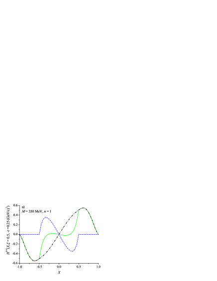
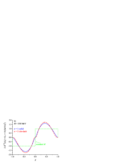
Figure 2: Skewed pion distribution $H^{I=0}$ for $t<0$ and in the forward limit.

The quark distributions calculated in this way correspond to some low normalization scale $Q_{0}$ which is of the order of a few hundred MeV . In order to make contact with the existing analysis of the pion nucleon data $\!{}^{{\bf?}}$ at $Q=2$ GeV, we have evolved the distributions depicted in Fig.2b starting from two different scales $Q_{0}=450$ and $350$ MeV. The results are plotted in Fig.3a together with the two parameterizations of the experimental data $\!{}^{{\bf?}}$: GRS and SMRS. The dashed (green, DR-A) line corresponds to the constant $M.$ Surprisingly the latter fits the experimental analysis the best $\!{}^{{\bf?}}$. It would be of interest to calculate the Drell-Yan cross section directly using the model qurak distributions and compare with the data.

Finally in Fig.3b we show the pion electromagnetic form-factor calculated by means of Eq.(7), which – as we checked explicitly – does not depend on $\xi$. One can see from Fig.3b that the theoretical curve overshoots the experimental points.

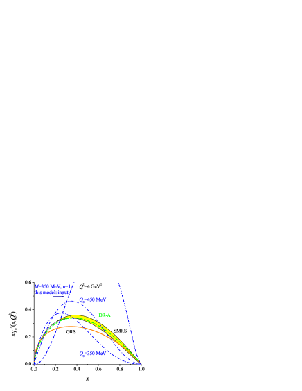
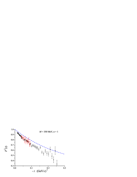
Figure 3: Quark distributions and pion electromagnetic form-factor

4 Concluding remarks

In calculating the pion skewed distributions we have relied on the definition (4) without taking into account that the currents in the non-local theories acquire additional terms $\!{}^{{\bf?}}$. It is of importance to investigate the impact of these new terms on our results. Pion structure function has been calculated in a similar model but in a different way in Ref.[10]. An alternative approach consists in calculating entire amplitude in the effective model $\!{}^{{\bf?}}$ without any reference to the factorization theorems.

References

References

-
[1]
E.B. Dally et al., Phys. Rev. Lett. 48, 375
(1982),
S.R. Amendeola et al., Nucl. Phys. B48, 168 (1986). -
[2]
P.J. Sutton, A.D. Martin, R.G. Roberts and W.J. Stirling,
Phys. Rev. D45, 2349 (1992),
M. Glück, E. Reya and I. Schienbein, Eur.Phys.J. C10, 313 (1999) and references therein. -
[3]
X.-D. Ji, Phys. Rev. Lett. 78, 610 (1997);
Phys. Rev. D55, 7114 (1997);
A.V. Radyushkin Phys. Rev. D56, 5524 (1997); D59, 014030 (1999). - [4] D.I. Diakonov and V.Yu. Petrov, hep-ph/0009006 and references therein.
- [5] V.Yu. Petrov, M.V. Polyakov, R. Ruskov, C. Weiss and K. Goeke, Phys. Rev. D59, 114018 (1999); V.Yu. Petrov and P.V. Pobylitsa, hep-ph/9712203.
- [6] M. Praszałowicz and A. Rostworowski, Phys. Rev. D64, 074003 (2001); hep-ph/0111196; hep-ph/0202226.
- [7] M.V. Polyakov and Ch. Weiss, Phys.Rev. D60, 114017 (1999).
- [8] R.M. Davidson, E. Ruiz Arriola, Phys. Lett. B348, 163 (1995); hep-ph/0110291.
- [9] R. S. Plant, M. C. Birse, Nucl. Phys. A628,607 (1998); R.D. Bowler, M. C. Birse, Nucl. Phys. A582; 655 (1995); W. Broniowski, hep-ph/9909438.
- [10] T. Shigetani, K. Suzuki, H. Toki, Phys. Lett. B308, 383 (1993); Nucl. Phys. A579, 413 (1994).
- [11] A.E. Dorokhov and L. Tomio, Phys.Rev. D62, 014016 (2000); I.V.Anikin, A.E.Dorokhov and L.Tomio, Phys. Lett. B475, 361 (2000) and A.E. Dorokhov this proceedings.