The one-loop functional of chiral SU(2)

Abstract:

The one-loop functional for chiral SU(2) of Gasser and Leutwyler is extended to include up to three propagators. With this generating functional it is possible to calculate all amplitudes up to order $\phi^{6}$ to next-to-leading order in the low-energy expansion. An external pion is of order $\phi$ and a vector gauge boson is of order $\phi^{2}$. A check of the existing amplitudes for $\gamma\gamma\to\pi\pi$ is given. The one-loop amplitudes and the cross sections for four-pion production in $e^{+}e^{-}$ annihilation are calculated.

1 Introduction

In the low-energy region it is not possible to calculate cross sections by means of perturbative QCD because of the high value of the strong coupling constant. One has to use an effective theory. The corresponding theory in this context is called chiral perturbation theory (CHPT) [1, 2, 3, 4]. It incorporates all symmetries of QCD with the assumption of spontaneous breakdown of chiral symmetry (which is suggested by phenomenological and theoretical evidence [5]), but no other model dependent features. CHPT is nonperturbative in the sense that it is not an expansion in powers of the QCD coupling constant, but an expansion in powers of the external momenta.

For a theory with a spontaneously broken symmetry the Goldstone theorem [6] predicts the existence of massless particles, called Goldstone bosons. In case of CHPT these bosons are not massless because the chiral symmetry is not an exact symmetry, as the quarks have masses. The pions are the by far lightest pseudoscalar mesons and therefore they are identified as the Goldstone bosons of broken chiral SU(2). In CHPT the asymptotic states are not quarks, but pions (or in general pseudoscalar mesons). A spontaneously broken symmetry corresponds to a nonlinear realization a la Nambu-Goldstone [7].

In the calculation of amplitudes one has to include loops to increase the precision and to satisfy unitarity and analyticity [1]. CHPT is not renormalizable in the sense that each loop in the perturbation expansion produces ultraviolet divergences, which have to be renormalized with the help of counterterms of the appropriate order in the external momenta. The finite parts of the coupling constants occurring in the counterterms are not determined by chiral symmetry and must be obtained from experiment or calculated using resonance exchange or other assumptions. Each successive loop and the associated counterterms correspond to successively higher powers of momenta. The higher loops are expected to give only small corrections at appropriately low energies.

Gasser and Leutwyler have calculated the generating one-loop functional of chiral SU(2) including two propagators in the loop [2]. With this functional one can obtain all amplitudes with at most four external particles, where an external photon counts as two particles. In this article the functional is extended by including a third propagator. This extension makes it easy to analyse processes with up to six external particles. In the whole work equal masses for the two lightest quarks are assumed.

The main purpose of calculations in the framework of pure CHPT is to analyse physics and to investigate QCD in a region ($E<<1$ GeV) where a perturbative treatment is not possible. CHPT was used successfully to study the low-energy structure of, e.g., $\pi\pi$ scattering [8] or of the pion form factor [9]. There are also important processes with more external particles. One example for an interesting process with six external particles is the scattering $e^{+}e^{-}\to 4\pi$, which is analysed in Sec. 5. It is an important cross section for determining the hadronic contribution to the anomalous magnetic moment of the muon and to the fine-structure constant at $M_{Z}$.

In Sec. 2 a calculation method with external fields [2] is introduced. The generating functional is given in Sec. 3. The amplitudes of the two channels of $\gamma\gamma\to\pi\pi$ [10, 11, 12] are presented in Sec. 4. In Sec. 5 the amplitudes and cross sections of the processes $e^{+}e^{-}\to\pi^{0}\pi^{0}\pi^{+}\pi^{-}$ and $e^{+}e^{-}\to 2\pi^{+}2\pi^{-}$ are provided. Sec. 6 contains some conclusions.

2 Matrix elements

The Lagrangian of massless QCD does not include any terms which connect the right- and left-handed components of the quark fields

$$q_{R}=\frac{1}{2}(1+\gamma_{5})q\,,\;\;\;\;\;q_{L}=\frac{1}{2}(1-\gamma_{5})q~{}.$$ (1)

Thus, the Lagrangian is invariant under chiral rotations, i.e. under two independent U$(N_{f})$ transformations (flavour rotations) of the right- and left-handed quark fields. In case of two flavours the Noether currents associated with chiral symmetry are given by :

$$J^{\mu 0}_{I}=\overline{q}_{I}\gamma^{\mu}q_{I}~{},\;\;\;\;\;J^{\mu a}_{I}=\overline{q}_{I}\gamma^{\mu}\frac{\tau_{a}}{2}q_{I}~{},\;\;\;\;\;I=L,R~{}.$$ (2)

The axial and vector currents are defined through the following relations:

$$V^{\mu a}=J^{\mu a}_{R}+J^{\mu a}_{L}\;\;\;\;\;\mbox{vector current}~{},$$ (3)

$$A^{\mu a}=J^{\mu a}_{R}-J^{\mu a}_{L}\;\;\;\;\;\mbox{axial current}~{}.$$ (4)

Because of Lorentz invariance and isospin symmetry there is the following relation:

$$<0|A^{\lambda}_{a}(x)|\pi_{b}(p)>=\mbox{i}\,p^{\lambda}\delta_{ab}F\,\mbox{e}^{-\mbox{\tiny i}\,p\cdot x}~{}.$$ (5)

Since chiral symmetry is spontaneously broken the Goldstone theorem insures that the constant $F$, which is related to the physical pion decay constant $F_{\pi}=$92.4 MeV through

$$F_{\pi}=F(1+{\cal O}(m_{quark}))~{},$$ (6)

is not zero. As a consequence the axial current, or the divergence of the axial current, plays the role of an interpolating field for the pion.

An external photon couples to the vector current. For example, the matrix element of the scattering $\gamma^{*}\rightarrow 4\pi$ is proportional to the on-shell residue of the corresponding singularity in the Green function

$$<\!0|\mbox{T}\,V^{\mu}_{n}(x_{1})A^{\nu}_{o}(x_{2})A^{\lambda}_{p}(x_{3})A^{\rho}_{q}(x_{4})A^{\sigma}_{r}(x_{5})|0\!>~{}.$$ (7)

To get such matrix elements one can use the method of external fields [2], which is equivalent to the method of external currents introduced by Schwinger [13]. Extra terms are added to the QCD Lagrangian:

$${\cal L}_{QCD}=\overline{q}\>\mbox{i}\gamma_{\mu}\nabla^{\mu}q-\frac{1}{2}\,\mbox{tr}_{c}F_{\mu\nu}F^{\mu\nu}+V_{\mu n}v^{\mu}_{n}+A_{\mu n}a^{\mu}_{n}-S_{n}s_{n}+P_{n}p_{n}~{}.$$ (8)

$\nabla^{\mu}$ is the SU(3)_C-covariant derivative. The external fields $v_{\mu}$, $a_{\mu}$, and $p$ are set to zero at the end of the calculation. The scalar field $s$ is set equal to the quark mass matrix to give masses to the light quarks, which amounts to explicit symmetry breaking. $S_{n}$ and $P_{n}$ are the scalar and pseudoscalar currents:

$$S_{0}=\bar{q}q~{},$$

$$S_{i}=\bar{q}\tau_{i}q\;\;\;\;\;\mbox{for}\;\;\>i=1,2,3~{},$$

$$P_{0}=\mbox{i}\,\bar{q}\gamma_{5}q~{},$$

$$P_{i}=\mbox{i}\,\bar{q}\gamma_{5}\tau_{i}q\;\;\;\;\;\mbox{for}\;\>i=1,2,3~{}.$$ (9)

By adding those terms in Eq. (8), the global chiral symmetry of the Lagrangian is promoted to a local symmetry with the appropriate gauge transformation [2]. The external field method allows the calculation of Green functions like (7) in an easy way. The generating functional of the Green functions is of the form:

$$W[v,a,s,p]\doteq\,<\!0|\mbox{T}\mbox{e}^{\mbox{\tiny i}\int d^{4}x\,V_{\mu n}(x)v^{\mu}_{n}(x)+A_{\mu n}(x)a^{\mu}_{n}(x)-S_{n}(x)s_{n}(x)+P_{n}(x)p_{n}(x)}|0\!>~{}.$$ (10)

One gets the Green functions by functional differentiation with respect to external fields, for example:

$$\left.\frac{\delta^{3}\,\mbox{i}\,W[v,a,s,p]}{\mbox{i}^{3}\delta a^{\lambda}_{p}(x_{1})\delta a^{\rho}_{q}(x_{2})\delta v^{\mu}_{r}(x_{3})}\right|_{\stackrel{{\scriptstyle v=0,a=0}}{{\scriptscriptstyle s={\cal M},p=0}}}=<\!0|\mbox{T}\,A_{\lambda p}(x_{1})A_{\rho q}(x_{2})V_{\mu r}(x_{3})|0\!>~{}.$$ (11)

The external fields can be interpreted as fields of external particles:

$$v^{\mu}+a^{\mu}=-e\,Q{\cal A}^{\mu}~{},$$ (12)

$$v^{\mu}-a^{\mu}=-e\,Q{\cal A}^{\mu}-\frac{e}{\sqrt{2}\sin\theta_{W}}(W^{\mu^{+}}T_{+}+\mbox{h.c.})~{}.$$ (13)

${\cal A}^{\mu}$ is the photon field, $W^{\mu^{+}}$ the W-boson field, $Q$ the charge matrix and $T_{+}$ contains the relevant elements of the Kobayashi-Maskawa matrix.

Because of the large value of the strong coupling constant in the low-energy region it is not possible to calculate the generating functional by means of perturbative QCD. So one has to use an effective Lagrangian that includes all possible terms built out of the matrix $U(\phi)$ (which contains the pion fields) and the external fields that respect all existing symmetries, namely chiral symmetry, Lorentz invariance, charge conjugation and parity. The corresponding Lagrangians given by Gasser and Leutwyler [2, 3] are the foundation of CHPT. In case of SU(2) and up to order $p^{4}$ ($p$ stands for the external momenta) one has:

$${\cal L}_{2}=\frac{F^{2}}{4}\langle D_{\mu}U^{\dagger}D^{\mu}U+\chi^{\dagger}U+\chi U^{\dagger}\rangle\,,$$ (14)

$${\cal L}_{4}= \frac{1}{4}\,l_{1}\,\langle D_{\mu}U^{\dagger}D^{\mu}U\rangle^{2}+\frac{1}{4}\,l_{2}\,\langle D_{\mu}U^{\dagger}D_{\nu}U\rangle\langle D^{\mu}U^{\dagger}D^{\nu}U\rangle+$$ (15)

$$+\frac{1}{16}\,l_{3}\,\langle\chi^{\dagger}U+\chi U^{\dagger}\rangle^{2}+\frac{1}{4}\,l_{4}\,\langle D_{\mu}U^{\dagger}D^{\mu}\chi+D_{\mu}UD^{\mu}\chi^{\dagger}\rangle+$$

$$+l_{5}\,\langle U^{\dagger}F_{\mu\nu}^{R}UF^{L\,\mu\nu}\rangle+\frac{\mbox{i}}{4}\,l_{6}\,\langle F_{\mu\nu}^{R}\,[D^{\mu}U,D^{\nu}U^{\dagger}]+F_{\mu\nu}^{L}\,[D^{\mu}U^{\dagger},D^{\nu}U]\rangle+$$

$$-\frac{1}{16}\,l_{7}\,\langle\chi^{\dagger}U-\chi U^{\dagger}\rangle^{2}+\frac{1}{4}\,h_{1}\,\langle\chi\chi^{\dagger}+\frac{1}{2}(\chi\tilde{\chi}-\chi^{\dagger}\tilde{\chi}^{\dagger})\rangle+$$

$$-(2h_{2}+\frac{l_{5}}{2})\,\langle F_{\mu\nu}^{R}F^{\mu\nu R}+F_{\mu\nu}^{L}F^{\mu\nu L}\rangle+\frac{1}{4}\,h_{3}\,\langle\chi\chi^{\dagger}-\frac{1}{2}(\chi\tilde{\chi}-\chi^{\dagger}\tilde{\chi}^{\dagger})\rangle~{}.$$

There are different possible parametrizations of $U(\phi)$, which all lead to the same on-shell amplitudes. A convenient choice is the exponential parametrization

$$U(\phi)=\,\mbox{exp}\,(\,\mbox{i}\,\phi/F)\,,\;\;\;\;\;\phi=\tau_{a}\phi_{a}=\left(\begin{array}[]{cc}\pi^{0}&\sqrt{2}\,\pi^{+}\\ \sqrt{2}\,\pi^{-}&-\pi^{0}\end{array}\right)\,.$$ (16)

The use of the covariant derivative

$$D_{\mu}U=\partial_{\mu}U-\mbox{i}\,r_{\mu}\,U+\mbox{i}\,U\,l_{\mu}\,,\;\;\;\;\;r_{\mu}=v_{\mu}+a_{\mu}\,,\;\;\;\;\;l_{\mu}=v_{\mu}-a_{\mu}$$ (17)

is a consequence of adding the extra terms in Eq. (8). The effective Lagrangians (14, 15) have the same local chiral symmetry as the extended QCD Lagrangian in (8). $\chi$ and $\tilde{\chi}$ are defined as follows:

$$\chi=2B(s+\mbox{i}\,p)~{},$$ (18)

$$\tilde{\chi}=\tau_{2}\,\chi^{T}\tau_{2}~{}.$$ (19)

$F$, $B$ and the $l_{i}$ are coupling constants. The Gell-Mann-Oakes-Renner relation, which can also be derived by CHPT, yields:

$$F^{2}M^{2}=-2\hat{m}\langle 0|\bar{u}u|0\rangle\,,\,\,\,\,\mbox{where}\,\,\,\hat{m}=(m_{u}+m_{d})/2~{}.$$ (20)

At a scale $\mu_{\overline{MS}}=1\mbox{ GeV }$, $\langle 0|\bar{u}u|0\rangle$ is approximately equal to -(230 MeV)³. Thus, $\hat{m}$ is assumed to be of order $M^{2}$:

$${\cal O}(\hat{m})={\cal O}(M^{2})={\cal O}(p^{2})~{}.$$ (21)

3 Calculation of the generating functional

CHPT can be defined via the path integral

$$W[v,a,s,p]\doteq{\cal N}^{-1}\int d\mu[U]\;\mbox{e}^{\mbox{\tiny i}\!\,\int\!d^{d}x\,{\cal L}_{\mbox{\tiny eff}}\,(v,a,s,p)}~{}.$$ (22)

The calculation is done in d dimensions so that dimensional regularisation can be used.

It can be shown that the loop expansion is an expansion in Planck’s constant or in other words an expansion around the solution of the classical equation of motion $\bar{U}=\bar{u}^{2}$. The matrix $U$ is expanded with the help of a traceless Hermitian matrix $\xi$:

$$U=u^{2}=\bar{u}\,\mbox{e}^{\mbox{i}\xi}\,\bar{u}~{}.$$ (23)

To the desired ${\cal O}(p^{4})$, the loop integration must only be performed over the Lagrangian of ${\cal O}(p^{2})$.

$$W={\cal N}^{-1}\mbox{e}^{\mbox{\tiny i}\!\,\int\!d^{d}x\,{\cal L}_{4}(\bar{U})}\int\!d\mu[\xi]\;\mbox{e}^{\mbox{\tiny i}\!\,\int\!d^{d}x\,{\cal L}_{2}(U)}+\dots~{}.$$ (24)

$d\mu[\xi]$ is the functional measure for the matrix field $\xi$. Planck’s constant is set equal to 1.

The Lagrangian is now expanded in $\xi$:

$$\int d^{d}x\,{\cal L}_{2}(U) = S_{2}[\bar{U}]+\frac{1}{4}F^{2}\int d^{d}x\,\langle D^{\mu}(\bar{u}^{\dagger}\xi\bar{u}^{\dagger})D_{\mu}(\bar{u}\xi\bar{u})-\frac{1}{2}D^{\mu}\bar{U}^{\dagger}D_{\mu}(\bar{u}\xi^{2}\bar{u})+$$ (25)

$$-\frac{1}{2}D^{\mu}\bar{U}D_{\mu}(\bar{u}^{\dagger}\xi^{2}\bar{u}^{\dagger})-\frac{1}{2}\xi^{2}(\bar{u}\chi^{\dagger}\bar{u}+\bar{u}^{\dagger}\chi\bar{u}^{\dagger})\rangle+{\cal O}(\xi^{3})~{}.$$

One has to consider the terms quadratic in $\xi$ for the one-loop calculation. $S_{2}[\bar{U}]$ is the classical action to order $p^{2}$. With the definitions

$$y_{\mu}\doteq\frac{1}{2}\bar{u}^{\dagger}D_{\mu}\bar{U}\bar{u}^{\dagger}=-\frac{1}{2}\bar{u}D_{\mu}\bar{U}^{\dagger}\bar{u}~{},$$ (26)

$$\Gamma_{\mu}\doteq\frac{1}{2}[\bar{u}^{\dagger},\partial_{\mu}\bar{u}]-\frac{1}{2}\mbox{i}\bar{u}^{\dagger}r_{\mu}\bar{u}-\frac{1}{2}\mbox{i}\bar{u}l_{\mu}\bar{u}^{\dagger}~{},$$ (27)

$$\sigma\doteq\frac{1}{2}(\bar{u}\chi^{\dagger}\bar{u}+\bar{u}^{\dagger}\chi\bar{u}^{\dagger})~{},$$ (28)

$$\hat{\Gamma}^{\mu\,ab}\doteq-\frac{1}{2}\langle[\tau^{a},\tau^{b}]\Gamma^{\mu}\rangle~{},$$ (29)

$$\hat{\sigma}^{ab}\doteq\frac{1}{2}\langle[\tau^{a},y_{\mu}][\tau^{b},y^{\mu}]\rangle+\frac{1}{4}\langle\{\tau^{a},\tau^{b}\}\sigma\rangle~{},$$ (30)

the generating functional of ${\cal O}(p^{4})$ has the form

$$W_{4}=\mbox{e}^{\mbox{\tiny i}\,(S_{2}[\bar{U}]+S_{4}[\bar{U}])}{\cal N}^{-1}\int\!d\mu[\xi]\;\mbox{e}^{-\mbox{\tiny i}\!\,\frac{F^{2}}{2}\int\!d^{d}x\,\xi^{a}(x){\cal D}^{ab}(x)\xi^{b}(x)}~{}.$$ (31)

The operator ${\cal D}$ is

$${\cal D}=\mbox{\bf 1}\Box+\{\hat{\Gamma}^{\mu},\partial_{\mu}\}+\hat{\Gamma}^{\mu}\hat{\Gamma}_{\mu}+\hat{\sigma}~{}.$$ (32)

The factor ${\cal N}$ is the one-loop integral with ${\cal D}$ replaced by ${\cal D}_{0}$

$${\cal D}^{ab}_{0}=\delta^{ab}\Box+\frac{1}{2}B\langle\{\tau^{a},\tau^{b}\}{\cal M}\rangle~{},$$ (33)

where ${\cal M}$ is the quark mass matrix $\hat{m}{\bf 1}$. With use of the Gaussian formula

$$\int d^{d}v\,\mbox{e}^{-\frac{1}{2}v^{T}Av}=(2\pi)^{\frac{d}{2}}(\mbox{det}\,A)^{-\frac{1}{2}}$$ (34)

one gets

$$W_{4}=\mbox{e}^{\mbox{\tiny i}\,(S_{2}+S_{4})}{(\det\frac{\cal D}{{\cal D}_{0}})}^{-\frac{1}{2}}~{}.$$ (35)

It is well known that one can define a generating functional $Z$ of all connected Green functions:

$$Z\doteq-\mbox{i}\,\mbox{ln}\,W~{},$$ (36)

$$Z_{4}=S_{2}+S_{4}+\frac{\mbox{i}}{2}\,\mbox{ln}\det\frac{\cal D}{{\cal D}_{0}}~{}.$$ (37)

With the identity ln det=Tr ln we have:

$$Z_{4}=S_{2}+S_{4}+\underbrace{\frac{\mbox{i}}{2}\,\mbox{Tr}\,\mbox{ln}\frac{\cal D}{{\cal D}_{0}}}_{\displaystyle Z_{\mbox{\scriptsize one loop}}}~{}.$$ (38)

In the further calculation the operator ${\cal D}$ is split into two parts:

$${\cal D}={\cal D}_{0}+\delta~{}.$$ (39)

With the quantity $\bar{\sigma}$ defined via

$$\bar{\sigma}\doteq\hat{\sigma}-2B\hat{m}\mbox{\bf 1}~{},$$ (40)

$\delta$ is of the form

$$\delta=\{\hat{\Gamma}^{\mu},\partial_{\mu}\}+\hat{\Gamma}^{\mu}\hat{\Gamma}_{\mu}+\bar{\sigma}~{}.$$ (41)

The one-loop functional can be rewritten as

$$Z_{\mbox{\scriptsize one loop}}=\frac{\mbox{i}}{2}\,\mbox{Tr}\,\mbox{ln}\frac{{\cal D}_{0}+\delta}{{\cal D}_{0}}=\frac{\mbox{i}}{2}\,\mbox{Tr}\,\mbox{ln}\,(\mbox{\bf 1}\,+\delta{\cal D}_{0}^{-1})=\frac{\mbox{i}}{2}\,\mbox{Tr}\,\mbox{ln}\,(\mbox{\bf 1}\,-\delta\Delta)~{}.$$ (42)

The Feynman propagator is the inverse of $-{\cal D}_{0}$. The logarithm is expanded as

$$\mbox{ln}\,(1+x)=\sum_{n=1}^{\infty}(-1)^{n-1}\frac{x^{n}}{n}~{}.$$ (43)

Gasser and Leutwyler have calculated the functional with at most two propagators in the loop [2]. In this work I extend it by including a third propagator. The functional is then of the form

$$Z_{\mbox{\scriptsize one loop}}=-\frac{1}{2}\,\mbox{i}\,\mbox{Tr}\,(\delta\Delta)-\frac{1}{4}\,\mbox{i}\,\mbox{Tr}\,(\delta\Delta\delta\Delta)-\frac{1}{6}\,\mbox{i}\,\mbox{Tr}\,(\delta\Delta\delta\Delta\delta\Delta)+{\cal O}(\phi^{8})~{}.$$ (44)

This means the functional is of order $\phi^{6}$ as there are at least two external pions on each vertex in the loop. The photon field can couple to a loop vertex without external pions and is therefore counted as order $\phi^{2}$.

The loop integrals contain the functions $A$, $B$ which have divergent parts that are proportional to a quantity $\Lambda(\mu)$:

$$\Lambda(\mu)=\frac{\mu^{d-4}}{(4\pi)^{2}}\mbox{\Large(}\frac{1}{d-4}-\frac{1}{2}(\mbox{ln}(4\pi)+\Gamma^{\prime}(1)+1)\mbox{\Large)}~{},$$ (45)

$$A(M^{2})=-\frac{M^{2}}{(4\pi)^{2}}\,\mbox{ln}\,\frac{M^{2}}{\mu^{2}}-2M^{2}\Lambda~{},$$ (46)

$$B(p^{2},M^{2})=\bar{B}(p^{2},M^{2})+B(0,M^{2})~{},$$ (47)

$$B(0,M^{2})=-\frac{1}{(4\pi)^{2}}\,(1+\mbox{ln}\,\frac{M^{2}}{\mu^{2}})-2\Lambda~{}.$$ (48)

The quantity $\mu$ is an arbitrary scale with the dimension of mass. With

$$\hat{\Gamma}^{\mu\nu}=\partial^{\mu}\hat{\Gamma}^{\nu}-\partial^{\nu}\hat{\Gamma}^{\mu}+[\hat{\Gamma}^{\mu},\hat{\Gamma}^{\nu}]$$ (49)

the one-loop functional has the following divergence structure [2, 3]:

$$Z_{\mbox{\scriptsize one loop}}^{\mbox{\scriptsize div}}=-\frac{\hat{\Lambda}}{12}\,\mbox{Tr}\,(\hat{\Gamma}^{\mu\nu}\hat{\Gamma}_{\mu\nu})-\frac{\hat{\Lambda}}{2}\,\mbox{Tr}\,(\hat{\sigma}\hat{\sigma})~{},$$ (50)

$$\hat{\Lambda}=\Lambda(\mu)+\frac{1}{32\pi^{2}}\,\mbox{ln}\,\frac{M^{2}}{\mu^{2}}~{},$$ (51)

$$\,\mbox{Tr}\,(\hat{\Gamma}^{\mu\nu}\hat{\Gamma}_{\mu\nu}) = -\frac{1}{2}\,\langle D_{\mu}\bar{U}^{\dagger}D^{\mu}\bar{U}\rangle^{2}+\frac{1}{2}\,\langle D_{\mu}\bar{U}^{\dagger}D_{\nu}\bar{U}\rangle\langle D^{\mu}\bar{U}^{\dagger}D^{\nu}\bar{U}\rangle+$$ (52)

$$-2\,\langle\bar{U}^{\dagger}F_{\mu\nu}^{R}\bar{U}F^{L\,\mu\nu}\rangle-\mbox{i}\,\langle F_{\mu\nu}^{R}\,[D^{\mu}\bar{U},D^{\nu}\bar{U}^{\dagger}]+F_{\mu\nu}^{L}\,[D^{\mu}\bar{U}^{\dagger},D^{\nu}\bar{U}]\rangle+$$

$$-\langle F_{\mu\nu}^{R}F^{\mu\nu R}+F_{\mu\nu}^{L}F^{\mu\nu L}\rangle~{},$$

$$\,\mbox{Tr}\,(\hat{\sigma}\hat{\sigma}) = \frac{1}{4}\,\langle D_{\mu}\bar{U}^{\dagger}D^{\mu}\bar{U}\rangle^{2}+\frac{1}{4}\,\langle D_{\mu}\bar{U}^{\dagger}D_{\nu}\bar{U}\rangle\langle D^{\mu}\bar{U}^{\dagger}D^{\nu}\bar{U}\rangle+$$ (53)

$$+\frac{1}{2}\,\langle D_{\mu}\bar{U}^{\dagger}D^{\mu}\bar{U}\rangle\langle\chi^{\dagger}\bar{U}+\chi\bar{U}^{\dagger}\rangle+\frac{3}{16}\,\langle\chi^{\dagger}\bar{U}+\chi\bar{U}^{\dagger}\rangle^{2}~{},$$

$$\langle D_{\mu}\bar{U}^{\dagger}D^{\mu}\bar{U}\rangle\langle\chi^{\dagger}\bar{U}+\chi\bar{U}^{\dagger}\rangle=2\,\langle D_{\mu}\bar{U}^{\dagger}D^{\mu}\chi+D_{\mu}\bar{U}D^{\mu}\chi^{\dagger}\rangle+$$

$$+2\,\langle\chi\chi^{\dagger}+\frac{1}{2}(\chi\tilde{\chi}-\chi^{\dagger}\tilde{\chi}^{\dagger})\rangle-\frac{1}{2}\,\langle\chi^{\dagger}\bar{U}+\chi\bar{U}^{\dagger}\rangle^{2}~{}.$$ (54)

The divergences can be eliminated by a renormalization of the coupling constants:

$$l_{i}=\tilde{l}_{i}+\gamma_{i}\,\hat{\Lambda}\,,\;\;\;\;\;h_{i}=\tilde{h}_{i}+\delta_{i}\,\hat{\Lambda}~{}.$$ (55)

The finite quantities $\tilde{l}_{i}$ and $\tilde{h}_{i}$ as well as the divergent $\hat{\Lambda}$ are scale independent. To absorb the divergences of the loops, the $\gamma_{i}$ and $\delta_{i}$ take the following values [2]:

$$\gamma_{1}=\frac{1}{3}\,,\;\;\;\;\;\gamma_{2}=\frac{2}{3}\,,\;\;\;\;\;\gamma_{3}=-\frac{1}{2}\,,\;\;\;\;\;\gamma_{4}=2\,,\;\;\;\;\;\gamma_{5}=-\frac{1}{6}\,,\;\;\;\;\;$$

$$\gamma_{6}=-\frac{1}{3}\,,\;\;\;\;\;\gamma_{7}=0\,,\;\;\;\;\;\delta_{1}=2\,,\;\;\;\;\;\delta_{2}=\frac{1}{12}\,,\;\;\;\;\;\delta_{3}=0~{}.$$ (56)

The renormalization scheme amounts to the following replacements:

$$l_{i}\rightarrow\tilde{l}_{i}\,,\;\;\;\;\;h_{i}\rightarrow\tilde{h}_{i}\,,$$ (57)

$$A\rightarrow 0\,,\;\;\;\;\;B(p^{2})\rightarrow\bar{B}(p^{2})-\frac{1}{(4\pi)^{2}} ~{}.$$

All in all we have the renormalized one-loop functional

$$Z_{4}[U,a,v,s,p]=\int d^{4}x\,\mbox{\Large(}{\cal L}_{2}+{\cal L}^{ren}_{4}\mbox{\Large)}+$$

$$+\int d^{4}x\,d^{4}y\frac{d^{4}p}{(2\pi)^{4}}\,\mbox{e}^{-\mbox{\tiny i}p(x-y)}\,\mbox{\huge(}F_{1}^{\mu\nu}(p)\,\mbox{Sp}\mbox{\Large(}\hat{\Gamma}^{\mu}(x)\hat{\Gamma}^{\nu}(y)\mbox{\Large)}+$$

$$\;\;\;\;\;+F_{2}(p)\,\mbox{Sp}\mbox{\Large(}\bar{\sigma}(x)\bar{\sigma}(y)\mbox{\Large)}+F_{3}^{\mu\nu}(p)\,\mbox{Sp}\mbox{\Large(}\hat{\Gamma}^{\mu}(x)\hat{\Gamma}^{\nu}(x)\bar{\sigma}(y)\mbox{\Large)}\mbox{\huge)}+$$

$$+\int d^{4}x\,d^{4}y\,d^{4}z\frac{d^{4}p_{a}}{(2\pi)^{4}}\frac{d^{4}p_{b}}{(2\pi)^{4}}\,\mbox{e}^{\mbox{\tiny i}p_{a}(z-x)}\mbox{e}^{\mbox{\tiny i}p_{b}(y-z)}$$

$$\>\mbox{\huge(}F_{4}^{\mu\nu\lambda}(p_{a},p_{b})\,\mbox{Sp}\mbox{\Large(}\hat{\Gamma}^{\mu}(x)\hat{\Gamma}^{\nu}(y)\hat{\Gamma}^{\lambda}(z)\mbox{\Large)}+F_{5}^{\mu\nu}(p_{a},p_{b})\>\>\>\mbox{Sp}\mbox{\Large(}\hat{\Gamma}^{\mu}(x)\hat{\Gamma}^{\nu}(y)\bar{\sigma}(z)\mbox{\Large)}$$

$$\;\;\;\;\;+F_{6}^{\mu}(p_{a},p_{b})\>\>\>\mbox{Sp}\mbox{\Large(}\bar{\sigma}(x)\bar{\sigma}(y)\hat{\Gamma}^{\mu}(z)\mbox{\Large)}+F_{7}(p_{a},p_{b})\,\mbox{Sp}\mbox{\Large(}\bar{\sigma}(x)\bar{\sigma}(y)\bar{\sigma}(z)\mbox{\Large)}\mbox{\huge)}~{}.$$ (58)

Figure 1: Definition of external momenta.

${\cal L}^{ren}_{4}$ is the Lagrangian of Eq. (15) with the $l_{i}$ and $h_{i}$ replaced by the $\tilde{l}_{i}$ and $\tilde{h}_{i}$. The scale dependence of the renormalized ${\cal O}(p^{4})$-coupling constants has cancelled the chiral logs of the loops. So everything is scale independent as it should be. The constituent functions $F_{1}^{\mu\nu}\,,\,\dots\,,\,F_{7}$ can be found in App. A. Sp denotes the trace in the space of the 3$\times$3 matrices in the adjoint representation. The external momenta flow as shown in Fig. 1.

The loop part is of order $p^{4}$ as one can see by dimensional considerations [1]. With ${\cal L}_{2}$ and ${\cal L}_{4}$ containing all possible terms respecting the symmetries of QCD, $Z_{4}$ is the complete generating functional of ${\cal O}(p^{4})$ for Green functions of quark currents. In the context of SU(2)$\times$SU(2) there is no anomalous part in the generating functional.

4 Amplitudes for $\gamma\gamma\to\pi\pi$

In case of pions and photons one can use the following recipe to extract the scattering amplitudes from the generating functional [14]:

• Expand all quantities which contain the matrices $\bar{U}(\phi)$ or $\bar{u}(\phi)$ in the pion fields.

• Replace the external fields $\chi$ by $M$, $a_{\mu}$ by zero and $v_{\mu}$ by $-e\,Q{\cal A}_{\mu}$ ($Q$ is the quark mass matrix, ${\cal A}_{\mu}$ is the photon field).

• Perform functional differentiation with respect to the external pion and photon fields.

This method is equivalent to the method described in Sec. 2 because the pion matrix is determined by the equation of motion in the following way

$$\phi=(\Box+M^{2})^{-1}F\,\partial_{\mu}a^{\mu}+\dots\,,$$ (59)

and only pole contributions are relevant for scattering amplitudes.

The amplitude of the process $\gamma(k_{1})\gamma(k_{2})\rightarrow\pi^{0}\pi^{0}$ ($s=(k_{1}+k_{2})^{2}$) is given by

$${\cal M}_{\gamma\gamma\to\pi^{0}\pi^{0}}=\frac{4\,e^{2}}{F_{\pi}^{2}}\left(F^{\mu\nu}_{3}(k_{1}+k_{2})+F^{\mu\nu}_{5}(k_{1},-k_{2})\right)\epsilon_{1\mu}\epsilon_{2\nu}\left(s-M_{\pi}^{2}\right)\,.$$ (60)

This can be simplified to

$${\cal M}_{\gamma\gamma\to\pi^{0}\pi^{0}}=\epsilon_{1}\cdot\epsilon_{2}\,\frac{-e^{2}}{8\pi^{2}F^{2}_{\pi}}(s-M^{2}_{\pi})\left(1+\frac{M^{2}_{\pi}}{s}\left(\mbox{ln}\left(\frac{1+\sqrt{1-\frac{4M^{2}_{\pi}}{s}}}{1-\sqrt{1-\frac{4M^{2}_{\pi}}{s}}}\right)-\mbox{i}\,\pi\right)^{2}\right)~{}.$$ (61)

The physical quantities $M_{\pi},F_{\pi}$ are obtained through the following renormalization:

$$M_{\pi}^{2} = M^{2}(1+\frac{2M^{2}}{F^{2}}\,\tilde{l}_{3})+{\cal O}(p^{6})\,,$$

$$F_{\pi} = F(1+\frac{M^{2}}{F^{2}}\,\tilde{l}_{4})+{\cal O}(p^{6})\,.$$ (62)

In this case, where the amplitude starts at order $p^{4}$, the difference between using $M$, $F$ and $M_{\pi}$, $F_{\pi}$ would appear first at order $p^{6}$. The amplitude (61) is equal to the one in [10].

In case of $\gamma(k_{1})\gamma(k_{2})\rightarrow\pi^{+}(p_{A})\pi^{-}(p_{B})$ one has:

$${\cal M}_{\gamma\gamma\to\pi^{+}\pi^{-}}=2\,e^{2}\left(a\,\epsilon_{1}\cdot\epsilon_{2}-\frac{p_{A}\cdot\epsilon_{1}\,p_{B}\cdot\epsilon_{2}}{p_{A}\cdot k_{1}}-\frac{p_{A}\cdot\epsilon_{2}\,p_{B}\cdot\epsilon_{1}}{p_{A}\cdot k_{2}}\right)~{},$$ (63)

$$a = 1+\frac{s}{F^{2}_{\pi}}\,(2\tilde{l}_{5}-\tilde{l}_{6})+\frac{2}{F_{\pi}^{2}}\left(F^{\mu\nu}_{3}(k_{1}+k_{2})+F^{\mu\nu}_{5}(k_{1},-k_{2})\right)\epsilon_{1\mu}\epsilon_{2\nu}\,s$$

$$= 1+\frac{s}{F^{2}_{\pi}}\,(2\tilde{l}_{5}-\tilde{l}_{6})-\frac{1}{32\pi^{2}F^{2}_{\pi}}\left(s+M^{2}_{\pi}\left(\mbox{ln}\left(\frac{1+\sqrt{1-\frac{4M^{2}_{\pi}}{s}}}{1-\sqrt{1-\frac{4M^{2}_{\pi}}{s}}}\right)-\mbox{i}\,\pi\right)^{2}\right)~{}.$$

This result agrees with the pion part of the amplitude in [11] and with the ${\cal O}(p^{4})$ part in [12].

5 Amplitudes and cross sections for $e^{+}e^{-}\to 4\pi$

The amplitude for the scattering

$$e^{+}(k_{+})e^{-}(k_{-})\to\pi^{0}(p_{1})\pi^{0}(p_{2})\pi^{+}(p_{3})\pi^{-}(p_{4})$$

takes the following form

$${\cal M}_{e^{+}e^{-}\to 2\pi^{0}\pi^{+}\pi^{-}}=\displaystyle\frac{e^{2}}{q^{2}+i\varepsilon}\overline{v}(k_{+})\gamma_{\mu}u(k_{-})J^{\mu}(p_{1},p_{2},p_{3},p_{4})~{},\hskip 11.38092ptq=k_{+}+k_{-}=\displaystyle\sum_{i=1}^{4}p_{i}~{},$$ (65)

$$J^{\mu}(p_{1},p_{2},p_{3},p_{4}):=\langle\pi^{0}(p_{1})\pi^{0}(p_{2})\pi^{+}(p_{3})\pi^{-}(p_{4})|J^{\mu}_{\rm elm}(0)|0\rangle~{}.$$ (66)

Because of Bose symmetry and $C$ invariance, $J^{\mu}$ can be written [15] as

$$J^{\mu}(p_{1},p_{2},p_{3},p_{4}) = A^{\mu}(p_{1},p_{2},p_{3},p_{4})+A^{\mu}(p_{2},p_{1},p_{3},p_{4})$$ (67)

$$-A^{\mu}(p_{1},p_{2},p_{4},p_{3})-A^{\mu}(p_{2},p_{1},p_{4},p_{3})~{}.$$

To next-to-leading order in CHPT, the reduced amplitude $A^{\mu}(p_{1},p_{2},p_{3},p_{4})$ contains the tree amplitudes of ${\cal O}(p^{2})$ and ${\cal O}(p^{4})$ and the one-loop part:

$$A^{\mu}=A^{\mu}_{(2)}+A^{\mu}_{(4){\rm tree}}+A^{\mu}_{(4){\rm loop}}~{}.$$ (68)

In some cases it is convenient to use kinematic variables in the amplitude:

$$s=(p_{1}+p_{2})^{2}~{},\;\;\;\;\;\nu=(p_{3}-p_{4})\cdot(p_{1}-p_{2})/2~{},$$

$$t_{i}=p_{i}\cdot q~{}~{}(i=1,\dots,4)~{}.$$ (69)

In the following I drop terms proportional to $q^{\mu}$ because they cannot contribute to the differential cross section of electroproduction. One can recover them with the help of current conservation. The amplitude $A^{\mu}$ is given by:

$$A^{\mu}_{(2)}(p_{1},p_{2},p_{3},p_{4})=\displaystyle\frac{s-M_{\pi}^{2}}{F_{\pi}^{2}}\displaystyle\frac{p_{3}^{\mu}}{2t_{3}-q^{2}}~{},$$ (70)

$$F_{\pi}^{4}A^{\mu}_{(4){\rm tree}}(p_{1},p_{2},p_{3},p_{4}) = 2\widetilde{l}_{2}(\nu-t_{3})p_{1}^{\mu}$$

$$+\left\{2\widetilde{l}_{1}(s^{2}-4sM_{\pi}^{2}+4M_{\pi}^{4})+\displaystyle\frac{\widetilde{l}_{2}}{2}(s^{2}-2t_{1}t_{2}+2t_{1}^{2}-8t_{1}\nu+4\nu^{2}-(q^{2}-2t_{3})^{2})\right.$$

$$\left.+2\widetilde{l}_{3}M_{\pi}^{4}+2\widetilde{l}_{4}(sM_{\pi}^{2}-M_{\pi}^{4})+\widetilde{l}_{6}q^{2}(M_{\pi}^{2}-s)\right\}\displaystyle\frac{p_{3}^{\mu}}{2t_{3}-q^{2}}~{},$$

$$F_{\pi}^{4}A^{\mu}_{(4){\rm loop}}(p_{1},p_{2},p_{3},p_{4}) = \frac{2\,\left(3\,M_{\pi}^{2}+q^{2}-3\,s-2\,{t_{3}}\right)\,{{{p_{3}}}_{\nu}}\,{{F_{1}}}^{{\nu\mu}}(q^{2})}{3\,\left(2\,{t_{3}}-q^{2}\right)}$$ (72)

$$+\left(\frac{{{{p_{3}}}^{\mu}}}{2\,{t_{3}}-q^{2}}\right)\mbox{\huge\{}\left[({{{p_{1}}}_{\rho}}-{{{p_{3}}}_{\rho}}+q_{\rho})\,{{{p_{2}}}_{\nu}}-({{{p_{1}}}_{\rho}}-{{{p_{3}}}_{\rho}}+q_{\rho})\,{{{p_{4}}}_{\nu}}\right]\,{{F_{1}}}^{{\rho\nu}}(q-{p_{1}}-{p_{3}})$$

$$+\left[{{{p_{1}}}_{\rho}}\,({{{p_{2}}}_{\nu}}-{{{p_{3}}}_{\nu}}+q_{\nu})-{{{p_{4}}}_{\rho}}\,({{{p_{2}}}_{\nu}}-{{{p_{3}}}_{\nu}}+q_{\nu})\right]\,{{F_{1}}}^{{\rho\nu}}({p_{1}}+{p_{4}})$$

$$+2\,\mbox{\Large[}\left(3\,M_{\pi}^{4}+4\,M_{\pi}^{2}\,\left(-{t_{4}}+{p_{3}}\cdot{p_{4}}\right)+4\,{p_{1}}\cdot{p_{2}}\,\left(M_{\pi}^{2}-{t_{4}}+{p_{3}}\cdot{p_{4}}\right)\right)\,{F_{2}}({p_{1}}+{p_{2}})$$

$$+4\,{p_{1}}\cdot{p_{4}}\,\left(-{t_{2}}+{p_{2}}\cdot{p_{3}}\right)\,{F_{2}}(-{p_{1}}-{p_{4}})\mbox{\Large]}\mbox{\huge\}}$$

$$-\frac{{{{p_{3}}}_{\nu}}\,{{F_{1}}}^{{\mu\nu}}(q)}{6}-{{{p_{3}}}_{\nu}}\,{{F_{1}}}^{{\mu\nu}}({p_{1}}+{p_{3}})-{{{p_{1}}}_{\nu}}\,{{F_{1}}}^{{\mu\nu}}({p_{1}}+{p_{4}})$$

$$-4\,\mbox{\Large[}\left(M_{\pi}^{2}+{p_{1}}\cdot{p_{2}}\right)\,{{{p_{3}}}^{\mu}}\,{F_{2}}({p_{1}}+{p_{2}})+{p_{1}}\cdot{p_{3}}\,{{{p_{2}}}^{\mu}}\,{F_{2}}({p_{1}}+{p_{3}})\mbox{\Large]}$$

$$-{p_{2}}\cdot{p_{4}}\,\left({{{p_{1}}}_{\nu}}-{{{p_{3}}}_{\nu}}\right)\,{{F_{3}}}^{{\mu\nu}}(q-{p_{1}}-{p_{3}})-\left(M_{\pi}^{2}+2\,{p_{1}}\cdot{p_{2}}\right)\,{{{p_{3}}}_{\nu}}\,{{F_{3}}}^{{\mu\nu}}(q-{p_{3}}-{p_{4}})$$

$$-\frac{3\,\mbox{i}}{4}\,\left({{{p_{1}}}_{\nu}}\,{{{p_{2}}}_{\lambda}}-{{{p_{3}}}_{\nu}}\,{{{p_{2}}}_{\lambda}}-{{{p_{1}}}_{\nu}}\,{{{p_{4}}}_{\lambda}}+{{{p_{3}}}_{\nu}}\,{{{p_{4}}}_{\lambda}}\right)\,{{F_{4}}}^{{\mu\nu\lambda}}(q,{p_{1}}+{p_{3}})$$

$${-{p_{2}}\cdot{p_{4}}\,\left({{{p_{1}}}_{\nu}}-{{{p_{3}}}_{\nu}}\right)\,{{F_{5}}}^{{\mu\nu}}(q,{p_{1}}+{p_{3}})-\left(M_{\pi}^{2}+2\,{p_{1}}\cdot{p_{2}}\right)\,{{{p_{3}}}_{\nu}}\,{{F_{5}}}^{{\mu\nu}}(q,{p_{3}}+{p_{4}})}$$

$$-\mbox{i}\,{p_{1}}\cdot{p_{3}}\,{p_{2}}\cdot{p_{4}}\,{{F_{6}}}^{\mu}(-{p_{1}}-{p_{3}},{p_{2}}+{p_{4}})\,.$$

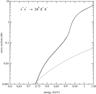
Figure 2: Theoretical predictions for the cross section $\sigma(e^{+}e^{-}\to 2\pi^{0}\pi^{+}\pi^{-})$ for 0.65 $\leq E$(GeV) $\leq$ 1.05.

The replacements $M\to M_{\pi}$ and $F\to F_{\pi}$ in the ${\cal O}(p^{2})$ part have given additional contributions to the ${\cal O}(p^{4})$ amplitudes.

With the complete amplitude one gets the differential cross section (setting $m_{e}=0$):

$$d\sigma=\displaystyle\frac{\alpha^{2}}{32\pi^{6}q^{6}}(\displaystyle\prod_{i=1}^{4}\frac{d^{3}p_{i}}{2E_{i}})\delta^{(4)}(q-\displaystyle\sum_{i=1}^{4}p_{i})l^{\mu\nu}J_{\mu}J_{\nu}^{*}\,.$$ (73)

One could perform the same calculations for the process $e^{+}e^{-}\to 2\pi^{+}2\pi^{-}$. In the isospin limit, which I assume in this article, it is a big simplification to use instead the following relation [16] that immediately gives the current matrix element for the $2\pi^{+}2\pi^{-}$ channel in terms of the matrix element for the $2\pi^{0}\pi^{+}\pi^{-}$ channel :

$$\langle\pi^{+}(p_{1})\pi^{+}(p_{2})\pi^{-}(p_{3})\pi^{-}(p_{4})|J^{\mu}_{\rm elm}(0)|0\rangle = J^{\mu}(p_{1},p_{3},p_{2},p_{4})+J^{\mu}(p_{1},p_{4},p_{2},p_{3})$$ (74)

$$+ J^{\mu}(p_{2},p_{3},p_{1},p_{4})+J^{\mu}(p_{2},p_{4},p_{1},p_{3})~{}.$$

Figure 3: Comparison of data [17] (left figure) and predictions (right figure, see text) for the cross section $\sigma(e^{+}e^{-}\to 2\pi^{+}2\pi^{-})$ for 0.65 $\leq E$(GeV) $\leq$ 1.05.

After numerical integration one gets the cross sections for the two channels. To be able to reach energies around 1 GeV, resonances have to be included as described in [15]. In Fig. 3 and Fig. 2 the dotted curve is the cross section for the $O(p^{4})$ amplitude, the full curve corresponds to the full amplitude with resonance exchange included and the dashed curve represents the complete amplitude without loops. As one can see, the influence of the loops is very small at higher energies. A detailed discussion of the results can be found in [15].

6 Conclusions

Chiral perturbation theory is the low-energy effective quantum field theory of QCD. It is characterized by chiral symmetry, by the identification of the lightest mesons as Goldstone bosons associated with the spontaneous breaking of the chiral symmetry and by explicit breaking of chiral symmetry via the masses of the light quarks. To parametrize the breaking terms induced by the quark masses, and also to generate in a systematic way the Green functions of quark currents, it is convenient to insert appropriate sources in the Lagrangian that promote the global chiral symmetry to a local symmetry.

One has to include loops to satisfy unitarity and to increase the precision. The loop expansion is an expansion in Planck’s constant, i.e an expansion around the solution of the classical equation of motion. The divergences coming from the loops have to be renormalized by counterterms of the corresponding order in the external momenta.

I gave a compact expression for the generating one-loop functional of chiral SU(2) in the isospin limit with at most three propagators in the loop. With this functional one can easily get all possible amplitudes up to order $\phi^{6}$, where an external pion is of order $\phi$ and a vector gauge boson is of order $\phi^{2}$.

With the help of the generating functional I calculated the processes $e^{+}e^{-}\to\pi^{0}\pi^{0}\pi^{+}\pi^{-}$ and $e^{+}e^{-}\to 2\pi^{+}2\pi^{-}$ that are relevant for the hadronic contribution to the anomalous magnetic moment of the muon and to the fine-structure constant at $M_{Z}$. Apart from that I confirmed the existing results for $\gamma\gamma\rightarrow\pi^{0}\pi^{0}$ and $\gamma\gamma\rightarrow\pi^{+}\pi^{-}$ [10, 11, 12]. Other processes that can be calculated with the functional would be, for example, $\gamma^{*}\rightarrow\pi\pi\gamma$ or $\pi\pi\to\pi\pi\pi\pi$.

The corresponding calculation of the generating functional for the symmetry group SU(3)$\times$SU(3) (which allows also $K,\,\eta\,$ to occur as external particles) including the nonleptonic weak interactions [18] is under way.

Appendix A Constituent functions

The constituent functions of the one-loop functional are of the following form:

$$F_{1}^{\mu\nu}(p)=p^{\mu}p^{\nu}\,a(p^{2})+g^{\mu\nu}\,b(p^{2})\,,$$

$$F_{2}(p)=\frac{1}{4}B(p^{2})\,,\;\;\;\;\;F_{3}^{\mu\nu}(p)=\frac{1}{2}g^{\mu\nu}B(p^{2})\,,$$

$$F_{4}^{\mu\nu\lambda}(p_{a},p_{b})=\mbox{i}\,\mbox{\Large(}c_{a}p_{a}^{\mu}p_{a}^{\nu}p_{a}^{\lambda}+c_{b}p_{b}^{\mu}p_{b}^{\nu}p_{b}^{\lambda}+d_{a}p_{a}^{\mu}p_{a}^{\nu}p_{b}^{\lambda}$$

$$\;\;\;\;\;+e_{a}p_{a}^{\mu}p_{b}^{\nu}p_{a}^{\lambda}+f_{a}p_{b}^{\mu}p_{a}^{\nu}p_{a}^{\lambda}+d_{b}p_{b}^{\mu}p_{b}^{\nu}p_{a}^{\lambda}+f_{b}p_{b}^{\mu}p_{a}^{\nu}p_{b}^{\lambda}$$

$$\;\;\;\;\;+e_{b}p_{a}^{\mu}p_{b}^{\nu}p_{b}^{\lambda}+g_{a}p_{a}^{\mu}g^{\nu\lambda}+h_{a}p_{a}^{\nu}g^{\mu\lambda}+i_{a}p_{a}^{\lambda}g^{\mu\nu}$$

$$\;\;\;\;\;+h_{b}p_{b}^{\mu}g^{\nu\lambda}+g_{b}p_{b}^{\nu}g^{\mu\lambda}+i_{b}p_{b}^{\lambda}g^{\mu\nu}\mbox{\Large)}\,,$$

$$F_{5}^{\mu\nu}(p_{a},p_{b})=j_{a}g^{\mu\nu}+k_{a}p_{a}^{\mu}p_{a}^{\nu}+k_{b}p_{b}^{\mu}p_{b}^{\nu}$$

$$\;\;\;\;\;+l_{a}p_{a}^{\mu}p_{b}^{\nu}+m_{a}p_{b}^{\mu}p_{a}^{\nu}\,,$$

$$F_{6}^{\mu}(p_{a},p_{b})=\mbox{i}\,\mbox{\Large(}n_{a}p_{a}^{\mu}+n_{b}p_{b}^{\mu}\mbox{\Large)}\,,\;\;\;\;\;F_{7}(p_{a},p_{b})=\frac{1}{6}\,C\,,$$ (A.1)

with for example

$$c_{a}=c(p_{a}^{2},p_{b}^{2},p_{a}\cdot p_{b})\;\;\;\;\;\mbox{and}\;\;\;\;\;c_{b}=c(p_{b}^{2},p_{a}^{2},p_{a}\cdot p_{b})\,,$$ (A.2)

where

$$a(p^{2})=\frac{{B}(p^{2})-4\,{B_{22}}(p^{2})}{4}\,,\;\;\;\;\;b(p^{2})=-{B_{20}}(p^{2})\,,$$

$$c_{a}=\frac{{C_{11\,a}}-4\,C_{22\,a}+4\,{C_{33\,a}}}{3}\,,\;\;\;\;\;d_{a}=\frac{{C_{11\,a}}-2\,C_{22\,a}-2\,{{\tilde{C}}_{22}}+4\,{{\tilde{C}}}_{33\,a}}{3}\,,$$

$$e_{a}=\frac{-C/2+2\,{C_{11\,a}}+{C_{11\,b}}-2\,C_{22\,a}-4\,{{\tilde{C}}_{22}}+4\,{{\tilde{C}}}_{33\,a}}{3}\,,$$

$$f_{a}=\frac{-2\,\left({{\tilde{C}}_{22}}-2\,{{\tilde{C}}}_{33\,a}\right)}{3}\,,\;\;\;\;\;g_{a}=\frac{-2\,\left({C_{20}}-2\,{C_{31\,a}}\right)}{3}\,,\;\;\;\;\;h_{a}=\frac{4\,{C_{31\,a}}}{3}\,,$$

$$i_{a}=\frac{-2\,\left({C_{20}}-2\,{C_{31\,a}}\right)}{3}\,,\;\;\;\;\;j_{a}=-2\,{C_{20}}\,,\;\;\;\;\;k_{a}={C_{11\,a}}-2\,C_{22\,a}\,,$$

$$l_{a}=-\frac{{C}}{2}+{C_{11\,a}}+{C_{11\,b}}-2\,{{\tilde{C}}_{22}}\,,\;\;\;\;\;m_{a}=-2\,{{\tilde{C}}_{22}}\,,\;\;\;\;\;n_{a}=\frac{{C}}{2}-2\,{C_{11\,a}}~{}.$$ (A.3)

The B and C functions can be found in App. B.

Appendix B One-loop integrals

The functions $B$, $B_{ij}$, $C$ and $C_{ij}$ are defined through the following relations [19, 20, 21] ($C_{F}$ is the Feynman integration contour):

$$\{X\}\doteq\frac{1}{\mbox{i}}\int_{C_{F}}\frac{d^{d}k}{(2\pi)^{d}}\,\frac{X}{(k^{2}-M^{2})({(k-p)}^{2}-M^{2})}~{},$$ (A.4)

$$B(p^{2})=\{1\}~{},$$ (A.5)

$$\{k_{\mu}k_{\nu}\}=g_{\mu\nu}B_{20}(p^{2})+p_{\mu}p_{\nu}B_{22}(p^{2})~{},$$ (A.6)

$$\{\{X\}\}\doteq\frac{1}{\mbox{i}}\int_{C_{F}}\frac{d^{d}k}{(2\pi)^{d}}\,\frac{X}{(k^{2}-M^{2})({(k-p_{a})}^{2}-M^{2})({(k-p_{b})}^{2}-M^{2})}~{},$$ (A.7)

$$\{\{k_{\mu}\}\}=p_{a\mu}\,C_{11a}+p_{b\mu}\,C_{11b}~{},$$ (A.8)

$$C=\{\{1\}\}~{},$$ (A.9)

$$\{\{k_{\mu}k_{\nu}\}\}=g_{\mu\nu}\,C_{20}+p_{a\mu}p_{a\nu}\,C_{22a}+p_{b\mu}p_{b\nu}\,C_{22b}+(p_{a\mu}p_{b\nu}+p_{b\mu}p_{a\nu})\,\tilde{C}_{22}~{},$$ (A.10)

$$\{\{k_{\mu}k_{\nu}k_{\lambda}\}\} = p_{a\mu}p_{a\nu}p_{a\lambda}\,C_{33a}+p_{b\mu}p_{b\nu}p_{b\lambda}\,C_{33b}+$$ (A.11)

$$+(p_{a\mu}p_{a\nu}p_{b\lambda}+p_{a\mu}p_{b\nu}p_{a\lambda}+p_{b\mu}p_{a\nu}p_{a\lambda})\,\tilde{C}_{33a}+$$

$$+(p_{b\mu}p_{b\nu}p_{a\lambda}+p_{b\mu}p_{a\nu}p_{b\lambda}+p_{a\mu}p_{b\nu}p_{b\lambda})\,\tilde{C}_{33b}+$$

$$+(p_{a\mu}g_{\nu\lambda}+p_{a\nu}g_{\mu\lambda}+p_{a\lambda}g_{\mu\nu})\,C_{31a}+$$

$$+(p_{b\mu}g_{\nu\lambda}+p_{b\nu}g_{\mu\lambda}+p_{b\lambda}g_{\mu\nu})\,C_{31b}~{},$$

with $C_{ij\,a}=C_{ij}(p_{a}^{2},p_{b}^{2},p_{a}\cdot p_{b})$, $C_{ij\,b}=C_{ij}(p_{b}^{2},p_{a}^{2},p_{a}\cdot p_{b})$ and $C_{ij}=C_{ij\,a}=C_{ij\,b}$. The explicit form of the functions is

$$A(M^{2})=M^{2}\left(B(0,M^{2})+\frac{1}{16\pi^{2}}\right)\,,$$ (A.12)

$$B(p^{2},M^{2})=\bar{B}(p^{2},M^{2})+B(0,M^{2})\,,$$

$$\bar{B}(p^{2},M^{2})=\frac{1}{16\pi^{2}}\,\left(\sqrt{1-\frac{4(M^{2}-\mbox{i}\,\epsilon)}{p^{2}}}\,\mbox{ln}\,\frac{\sqrt{1-\frac{4(M^{2}-\mbox{\tiny i}\,\epsilon)}{p^{2}}}-1}{\sqrt{1-\frac{4(M^{2}-\mbox{\tiny i}\,\epsilon)}{p^{2}}}+1}+2\right)\,,$$ (A.13)

$$C(p_{a}^{2},p_{b}^{2},p_{a}\cdot p_{b},M^{2})=-\frac{1}{16\pi^{2}\sqrt{\lambda}}\sum^{3}_{i=1}\sum_{\sigma=\pm}\left(\mbox{Li}_{2}\left(\frac{x_{i}}{x_{i}-z_{i}^{\sigma}}\right)-\mbox{Li}_{2}\left(\frac{x_{i}-1}{x_{i}-z_{i}^{\sigma}}\right)\right)\,,$$

$$\lambda=4\left((p_{a}\cdot p_{b})^{2}-p_{a}^{2}p_{b}^{2}\right)\,,\;\;\;\;\;p_{D}^{2}=p_{a}^{2}-2p_{a}\cdot p_{b}+p_{b}^{2}\,,$$

$$x_{1}=\frac{1}{2}\left(1+\frac{p_{a}^{2}-p_{b}^{2}-p_{D}^{2}}{\sqrt{\lambda}}\right)\,,\;\;\;\;\;z_{1}^{\sigma}=\frac{1}{2}\left(1\pm\sqrt{1-\frac{4}{p_{a}^{2}}(M^{2}-\mbox{i}\,\epsilon)}\right)\,.$$ (A.14)

The quantities $x_{2}$, $z_{2}^{\sigma}$ are obtained by the interchange $p_{a}^{2}\leftrightarrow p_{D}^{2}$ and $x_{3}$, $z_{3}^{\sigma}$ by the interchange $p_{a}^{2}\leftrightarrow p_{b}^{2}$. Li₂ denotes the dilogarithm

$$\mbox{Li}_{2}(z)=-\int_{0}^{z}\frac{dt}{t}\mbox{ln}\,(1-t)\,.$$ (A.15)

The coefficients functions are of the form

$${B_{20}}(p^{2})=\frac{6\,M^{2}-p^{2}+48\,{\pi}^{2}\,A+24\,{\pi}^{2}\,\left(4\,M^{2}-p^{2}\right)\,B(p^{2})}{288\,{\pi}^{2}}\,,$$

$${B_{22}}(p^{2})=\frac{-6\,M^{2}+p^{2}+96\,{\pi}^{2}\,A-96\,{\pi}^{2}\,\left(M^{2}-p^{2}\right)\,B(p^{2})}{288\,p^{2}\,{\pi}^{2}}\,.$$ (A.16)

In the following $B(1)$ is defined as $B(p_{b}^{2})$ and $B(2)$ as $B(p_{a}^{2}-2\,p_{a}\cdot p_{b}+p_{b}^{2})$. The same is valid for $B_{20}$ and $B_{22}$.

$${C_{11\,a}}=\frac{{H_{11\,a}}\,{{p_{b}}}^{2}-{H_{11\,b}}\,{p_{a}\cdot p_{b}}}{{{p_{a}}}^{2}\,{{p_{b}}}^{2}-{{(p_{a}\cdot p_{b})}}^{2}}\,,$$

$${C_{20}}=\frac{2\,C\,M^{2}+\frac{1}{16\,{\pi}^{2}}+B(2)-{C_{11\,a}}\,{{p_{a}}}^{2}-{C_{11\,b}}\,{{p_{b}}}^{2}}{4}\,,$$

$${C_{22\,a}}=\frac{{H_{21\,a}}\,{{p_{b}}}^{2}-{H_{22\,b}}\,{p_{a}\cdot p_{b}}}{{{p_{a}}}^{2}\,{{p_{b}}}^{2}-{{(p_{a}\cdot p_{b})}}^{2}}\,,\;\;\;\;\;{{\tilde{C}}_{22}}=\frac{{H_{22\,b}}\,{{p_{a}}}^{2}-{H_{21\,a}}\,{p_{a}\cdot p_{b}}}{{{p_{a}}}^{2}\,{{p_{b}}}^{2}-{{(p_{a}\cdot p_{b})}}^{2}}\,,$$

$${C_{33\,a}}=\frac{{H_{31\,a}}\,{{p_{b}}}^{2}-{H_{32\,b}}\,{p_{a}\cdot p_{b}}}{{{p_{a}}}^{2}\,{{p_{b}}}^{2}-{{(p_{a}\cdot p_{b})}}^{2}}\,,\;\;\;\;\;{{{\tilde{C}}}_{33\,a}}=\frac{{H_{32\,b}}\,{{p_{a}}}^{2}-{H_{31\,a}}\,{p_{a}\cdot p_{b}}}{{{p_{a}}}^{2}\,{{p_{b}}}^{2}-{{(p_{a}\cdot p_{b})}}^{2}}\,,$$

$${C_{31\,a}}=\frac{{H_{30\,a}}\,{{p_{b}}}^{2}-{H_{30\,b}}\,{p_{a}\cdot p_{b}}}{{{p_{a}}}^{2}\,{{p_{b}}}^{2}-{{(p_{a}\cdot p_{b})}}^{2}}\,,$$

$${H_{11\,a}}=\frac{-B(1)+B(2)+C\,{{p_{a}}}^{2}}{2}\,,\;\;\;\;\;{H_{21\,a}}=-{C_{20}}+\frac{{B(2)}/{2}+{C_{11\,a}}\,{{p_{a}}}^{2}}{2}\,,$$

$${H_{22\,a}}=\frac{[{-B(1)+B(2)}]/{2}+{C_{11\,b}}\,{{p_{a}}}^{2}}{2}\,,\;\;\;\;\;{H_{30\,a}}=\frac{{C_{20}}\,{{p_{a}}}^{2}-{B_{20}}(1)+{B_{20}}(2)}{2}\,,$$

$${H_{31\,a}}=-2\,{C_{31\,a}}+\frac{{{p_{a}}}^{2}\,{C_{22\,a}}+{B_{22}}(2)}{2}\,,\;\;\;\;\;{H_{32\,a}}=\frac{{{p_{a}}}^{2}\,{C_{22\,b}}-{B_{22}}(1)+{B_{22}}(2)}{2}\,.$$

(A.17)

The divergent functions need to be renormalized as described in section 3.