Abstract

We perform a comprehensive study of the Higgs sector of the Minimal Supersymmetric extension of the Standard Model in the case where all Higgs bosons are rather light, with masses of ${\cal O}(100~{}{\rm GeV})$, and couple maximally to electroweak gauge bosons and strongly to standard third generation fermions, i.e. for large values of the ratio of the vacuum expectation values of the two Higgs doublet fields, $\tan\beta$. We first summarize the main phenomenological features of this “intense–coupling” scenario and discuss the available constraints from direct searches of Higgs bosons at LEP2 and the Tevatron as well as the indirect constraints from precision measurements such as the $\rho$ parameter, the $Zb\bar{b}$ vertex, the muon $(g-2)$ and the decay $b\to s\gamma$. We then analyze the decay branching fractions of the neutral Higgs particles in this regime and their production cross sections at the upcoming colliders, the Tevatron Run II, the LHC, a 500 GeV $e^{+}e^{-}$ linear collider (in the $e^{+}e^{-}$ and $\gamma\gamma$ options) as well as at a $\mu^{+}\mu^{-}$ collider.

1. Introduction

A firm prediction of the Minimal Supersymmetric Standard Model (MSSM) [1] is that, among the five scalar particles which are present in the extended Higgs sector [2], i.e.  two CP–even $h$ and $H$, a pseudoscalar $A$ and two charged $H^{\pm}$ bosons, at least the lightest Higgs boson $h$ must have a mass below $130$ GeV when radiative corrections are taken into account [?–?]. If the minimal version of Supersymmetry is indeed realized in Nature, this particle should be therefore accessible at the next generation of high–energy colliders, the high–luminosity Tevatron [6], the LHC [7, 8] and a future $e^{+}e^{-}$ linear collider [9, 10].

In the decoupling regime [11], that is when the Higgs bosons $H,A$ and $H^{\pm}$ are very heavy implying that they are almost degenerate in mass, $M_{A}\sim M_{H}\sim M_{H^{\pm}}$, the lightest Higgs particle $h$ will have the properties of the Standard Model (SM) Higgs boson. The experimental search for this particle will therefore be straightforward and there is now little doubt, in view of the detailed phenomenological and experimental analyses performed in the recent years, that it will not escape detection and that at least some of its fundamental properties can be pinned down. Unfortunately, the other MSSM Higgs bosons will have masses of ${\cal O}(1~{}{\rm TeV})$, and will therefore be too heavy to be accessible directly, implying that one would not be able to distinguish between the MSSM and the SM Higgs sectors.

An opposite and much more interesting situation would be the one where the mass of the pseudoscalar $A$ boson is not much larger than the maximal value allowed for $M_{h}$. In this case, the three neutral Higgs bosons $h,H$ and $A$ and the charged Higgs particles will have comparable masses, $M_{h}\sim M_{H}\sim M_{A}\raisebox{-3.69899pt}{~{}\shortstack{$<$ \\ [-0.07cm] $\sim$}}~{}130$ GeV and $M_{H^{\pm}}\raisebox{-3.69899pt}{~{}\shortstack{$<$ \\ [-0.07cm] $\sim$}}~{}150$ GeV. A particularly interesting scenario is when the parameter $\tan\beta$, the ratio of the vacuum expectation values of the two Higgs doublet fields which break the electroweak symmetry in the MSSM, is large, leading to a CP–even Higgs boson $\Phi_{A}$ [either $h$ or $H$] which is almost degenerate in mass with the pseudoscalar $A$ boson. As a consequence of the SUSY constraints on the Higgs sector, this CP–even $\Phi_{A}$ boson will have almost the same couplings as the $A$ boson, and therefore will couple strongly to the third generation $b$–quarks and $\tau$ leptons [since the couplings are proportional to $\tan\beta$], while the couplings of the $Z$–bosons to $\Phi_{A}A$ pairs [and the corresponding couplings of the $W$ bosons to $\Phi_{A}H^{\pm}$ pairs] will be maximal, i.e. not suppressed by (sine or cosine of) mixing angle factors. The other CP–even Higgs particle, that we will denote by $\Phi_{H}$, will have almost the couplings of the SM Higgs boson, i.e. its couplings to weak gauge bosons and to top quarks are not strongly suppressed by mixing angle factors and are therefore almost maximal.

This scenario, with all MSSM Higgs bosons being light with almost maximal couplings to gauge bosons and strong couplings to third generation fermions, will be called hereafter, the “intense–coupling” regime.

In this non–decoupling scenario, all three neutral Higgs bosons, as well as the charged Higgs particle, would be accessible at the next generation of experiments. The experimental searches for the neutral Higgs bosons in this case will be slightly more involved and much more interesting than in the decoupling regime, since a plethora of production and decay processes, with rates which can be violently different from the ones of the SM Higgs particles, have to be considered and studied in detail in order to detect individually all the three particles and to determine their basic properties. In addition, two features might render the situation somewhat more delicate: the $h,H,A$ boson masses can be very close to each other, implying that backgrounds for a given Higgs boson signal would come from another Higgs signal and the total decay widths of some of the Higgs bosons can be rather large [in particular for very large values of $\tan\beta$] implying broader signals.

The search for the charged Higgs particle would be straightforward. Indeed, since in the MSSM the $A$ and $H^{\pm}$ boson masses are related by $M_{H^{\pm}}^{2}\sim M_{A}^{2}+M_{W}^{2}$, $M_{H^{\pm}}$ will be smaller than $\sim 150$ GeV for $M_{A}\raisebox{-3.69899pt}{~{}\shortstack{$<$ \\ [-0.07cm] $\sim$}}~{}130$ GeV, implying that $H^{\pm}$ can always be produced in top quark decays, $t\to H^{+}b$, and can easily be detected at hadron [6, 7] or $e^{+}e^{-}$ colliders [9, 10].

The purpose of this paper is to perform a comprehensive study of the MSSM Higgs sector in the intense–coupling regime and the implications of the near mass degeneracy $M_{h}\sim M_{H}\sim M_{A}$, for the search of the Higgs bosons at the Tevatron, the LHC, a 500 GeV $e^{+}e^{-}$ collider and a $\mu^{+}\mu^{-}$ collider. We will first discuss the parameterization of the Higgs sector and derive rather simple, accurate and useful expressions for the radiative corrections to the Higgs masses and couplings which are valid in the region 90 GeV $\raisebox{-3.69899pt}{~{}\shortstack{$<$ \\ [-0.07cm] $\sim$}}~{}M_{A}\raisebox{-3.69899pt}{~{}\shortstack{$<$ \\ [-0.07cm] $\sim$}}~{}130$ GeV for moderate ($\sim 10)$ and large ($\sim 30$–50) $\tan\beta$ values. We will then analyze in this “intense–coupling” regime, the various decay branching ratios of the $h,H$ and $A$ particles and collect all their production cross sections at these machines. We will not only analyze the main production channels which allow to detect these particles, but also sub–leading processes which would allow for the measurement of some of their fundamental properties. The various experimental signatures for the Higgs particles will be discussed.

Before that, we will discuss in detail the various constraints on this intense–coupling regime with high $\tan\beta$ values: the direct constraints from the Tevatron and LEP2 searches for MSSM Higgs bosons [and the implications of the possible $\sim 2\sigma$ evidence [12] for a SM–like Higgs boson with a mass around 115 GeV] as well as all the indirect constraints from precision measurements [20, 21], i.e. the $W$ boson mass, the effective electroweak mixing angle $\sin^{2}\theta_{W}$ and the $Z$ boson decays into $\bar{b}b$ final states, the radiative decay $b\to s\gamma$ [22] and the anomalous magnetic moment of the muon, $(g-2)_{\mu}$ [23].

The paper is organized as follows. In the next section, we will present the physical set–up and summarize our parameterization of the MSSM Higgs sector, and display the Higgs boson masses and couplings in the intense–coupling regime. In section 3, we discuss the implications of the LEP2 and Tevatron direct Higgs searches and the indirect constraints from high precision measurements on this scenario. The various decay branching fractions of the neutral Higgs bosons will be analyzed in section 4. The production cross sections of the neutral Higgs bosons at the Tevatron, the LHC, a 500 GeV $e^{+}e^{-}$ linear collider and a $\mu^{+}\mu^{-}$ collider will be given in section 5, together with a discussion of the various processes and signatures which can be used. A conclusion will be given in section 6.

2. The MSSM Higgs sector and the intense–coupling regime

2.1 Radiative corrections in the Higgs sector

In the MSSM, besides the four Higgs boson masses, two mixing angles define the properties of the scalar particles and their interactions with gauge bosons and fermions: the ratio of the two vacuum expectation values $\tan\beta=v_{2}/v_{1}$ of the Higgs doublets and a mixing angle $\alpha$ in the neutral CP–even sector. Supersymmetry leads to several relations among these parameters and, in fact, only two of them, taken for convenience to be $M_{A}$ and $\tan\beta$, are independent. These relations impose, at the tree–level, a strong hierarchical structure on the mass spectrum [e.g. $M_{h}<M_{Z}$] some of which are, however, broken by radiative corrections. The leading part of these corrections grows as $m_{t}^{4}$ and logarithmically with the common stop mass $M_{S}$ [3]. Including the mixing in the stop and sbottom sectors and all the subleading terms, the full expressions of the radiative corrections become rather involved [4, 5].

To illustrate the qualitative behavior of the Higgs boson masses and couplings, we will use simple analytic expressions [comparable in simplicity to those obtained in [3] for the leading $m_{t}^{4}$ piece] where the stop mixing and some of the subleading terms are incorporated. In many cases, these expressions give rather good approximations for the neutral Higgs boson masses [at the percent level] and couplings [at the ten percent level] compared to what is obtained with the full set of corrections in the renormalization group improved approach of Ref. [4]. This is sufficient for our purpose in the present section, since our aim is simply to understand qualitatively the phenomenological implications of almost degenerate Higgs bosons with enhanced Yukawa couplings.

For our numerical analysis throughout the paper, we will use the program HDECAY [24], which calculates the Higgs spectrum and decay widths in the MSSM. The complete radiative corrections due to top/bottom quark and squark loops within the effective potential approach, leading NLO QCD corrections [through renormalization group improvement] and the full mixing in the stop and sbottom sectors are incorporated using the analytical expressions of Ref. [4]. [Note also that we will include the leading one–loop and two–loop corrections to the Higgs self–couplings.] However, even in this case, our treatment of the radiative corrections in the Higgs sector will not be complete, since two sets of potentially large corrections are presently not included in the program:

– The SUSY–QCD and dominant Yukawa radiative corrections to the bottom and top quark Yukawa couplings which, in many cases, can be rather important. In particular, the corrections to the bottom Yukawa couplings can be very large for high values of $\tan\beta$ and the higgsino mass parameter $\mu$ [25]. The net effect of these corrections can be viewed as an increase or decrease of the bottom quark mass, depending on the sign of $\mu$. The phenomenological impact of these corrections has been already discussed in the literature, see e.g. Ref. [18, 25], and we have little to add.

– Recently, the two–loop ${\cal O}(\alpha_{t}^{2})$ and ${\cal O}(\alpha_{s}\alpha_{b})$ Yukawa corrections to the Higgs boson masses have been calculated [26]. The former set of corrections can increase the lightest $h$ boson mass by several GeV in some areas of the MSSM parameter space, while the later corrections can be sizeable for large $\tan\beta$ values.

We have nevertheless verified that the numerical results that we obtain for the MSSM Higgs spectrum, and in particular for the lightest $h$ boson mass, are rather close to those obtained from the complete results of the Feynman diagrammatic approach implemented in the program FeynHiggs [27], which include some of the Yukawa corrections of Ref. [26]. The difference, of the order of a few GeV, is of the same size (within a factor of two) as the expected theoretical error on the determination of the Higgs boson masses. However, as already pointed out, this difference will not be of utmost importance for our analysis, and our general conclusions will not be altered in a significant way.

2.2 The Higgs boson masses

Before discussing the Higgs boson masses in the intense–coupling regime, i.e. when the $A$ boson is rather light and $\tan\beta$ is very large, let us first present the rather simple analytical expression which approximate the Higgs boson masses. We first define the quantity $\epsilon$, which parameterizes the main radiative correction,

$$\epsilon=\frac{3G_{F}\overline{m}_{t}^{4}}{\sqrt{2}\pi^{2}\sin^{2}\beta}\,\bigg{[}t+\frac{X_{t}}{2}\bigg{]}-\frac{3G_{F}}{\sqrt{2}\pi^{2}}\bigg{[}\frac{\overline{m}_{t}^{2}M_{Z}^{2}t}{2}+\frac{2\alpha_{S}}{\pi}\frac{\overline{m}_{t}^{4}}{\sin^{2}\beta}(X_{t}t+t^{2})\bigg{]}$$ (1)

with

$$t=\log\bigg{(}\frac{M_{S}^{2}}{m_{t}^{2}}\bigg{)}\ \ ,\ \ X_{t}=\frac{2A_{t}^{2}}{M_{S}^{2}}\bigg{(}1-\frac{A_{t}^{2}}{12M_{S}^{2}}\bigg{)}\hskip 42.67912pt$$

where $\overline{m}_{t}$ is the running ${\rm\overline{MS}}$ top quark mass to account for the leading QCD corrections, $A_{t}$ is the stop trilinear coupling, and $\alpha_{S}$ the strong coupling constant. The Higgs boson masses can be approximated to an accuracy of the order of a few percent compared to the complete result [in particular in the case where the splitting between the two stop masses, and to a lesser extent sbottom masses, is not very large], as functions of $M_{A}$, $\tan\beta$ and $\epsilon$ with the expression

$$M_{h,H}^{2} = \frac{1}{2}(M_{A}^{2}+M_{Z}^{2}+\epsilon)\left[1\mp\sqrt{1-4\frac{M_{Z}^{2}M_{A}^{2}\cos^{2}2\beta+\epsilon(M_{A}^{2}\sin^{2}\beta+M_{Z}^{2}\cos^{2}\beta)}{(M_{A}^{2}+M_{Z}^{2}+\epsilon)^{2}}}\right]$$ (2)

This radiative correction pushes the maximum value of the lightest $h$ boson mass upwards from $M_{Z}$ by several tens of GeV: in the so–called maximal mixing scenario $\tilde{A}_{t}=A_{t}-\mu/\tan\beta=\sqrt{6}M_{S}$ and with $M_{A}$ and $M_{S}$ of about 1 TeV, one obtains an upper mass bound, $M_{h}\raisebox{-3.69899pt}{~{}\shortstack{$<$ \\ [-0.07cm] $\sim$}}~{}130$ GeV for $\tan\beta\gg 1$, a bound that is comparable to the one obtained including the full set of corrections in the RG improved approach [4].

In the case of the mixing angle $\alpha$ of the CP–even Higgs sector, the correction eq. (1) is not accurate enough and one needs to introduce another correction which involves the ratio $\mu/M_{S}$, where $\mu$ is the higgsino mass parameter. Defining the parameter $\epsilon^{\prime}$ to be

$$\epsilon^{\prime}=\frac{G_{F}\overline{m}_{t}^{4}}{2\sqrt{2}\pi^{2}\sin^{2}\beta}\frac{\mu}{M_{S}}\bigg{[}\frac{A_{t}^{3}}{M_{S}^{3}}-\frac{6A_{t}}{M_{S}}\bigg{]}\bigg{[}1-\frac{4\alpha_{S}t}{\pi}\bigg{]}$$ (3)

the mixing angle $\alpha$ is given in terms of $M_{A},\tan\beta,\epsilon$ and $\epsilon^{\prime}$, by

$$\tan 2\alpha=\tan 2\beta\,\frac{M_{A}^{2}+M_{Z}^{2}-\epsilon^{\prime}/\sin 2\beta}{M_{A}^{2}-M_{Z}^{2}+\epsilon/\cos 2\beta}\ ,\hskip 28.45274pt-\frac{\pi}{2}\leq\alpha\leq 0\ .$$ (4)

Here again, the accuracy of the formula, compared to the case where the full corrections are taken into account, is at the percent level if the splitting between the stop (and to a lesser extent, sbottom) masses is not too large.

[In the case of the charged Higgs boson mass, one can also derive a very simple expression for the radiative corrections which gives a result that is accurate at the percent level,

$$M_{H^{\pm}}=\sqrt{M_{A}^{2}+M_{W}^{2}-\epsilon_{+}}\ \ {\rm with}\ \ \epsilon_{+}=\frac{3G_{F}M_{W}^{2}t}{4\sqrt{2}\pi^{2}}\bigg{[}\frac{\overline{m}_{t}^{2}}{\sin^{2}\beta}+\frac{\overline{m}_{b}^{2}}{\cos^{2}\beta}\bigg{]}$$ (5)

where $\overline{m}_{b}$ is the running $\overline{\rm MS}$ $b$ mass at the scale of the top quark mass.]

Let us now discuss in some details the neutral Higgs boson masses in the intense–coupling regime, taking into account the dominant radiative corrections $\epsilon$ and $\epsilon^{\prime}$. In fact, this regime can be defined as the one where the two CP–even Higgs bosons $h$ and $H$ are almost degenerate in mass, $M_{h}\simeq M_{H}$. We will therefore first concentrate on the Higgs sector in the limit $M_{h}=M_{H}$.

Solving the equation (2) for $M_{H}^{2}-M_{h}^{2}=0$, which is a second order polynomial equation in the variable $M_{A}^{2}$,

$$M_{A}^{4}+2M_{A}^{2}[M_{Z}^{2}(1-2\cos^{2}2\beta)+\epsilon\cos 2\beta]+M_{Z}^{4}+\epsilon^{2}-2M_{Z}^{2}\epsilon\cos 2\beta=0$$ (6)

one obtains a discriminant $\Delta^{\prime}=-\sin^{2}2\beta(2M_{Z}^{2}\cos 2\beta-\epsilon)^{2}\leq 0$. The only way for the solution to be real is therefore to have either $\sin 2\beta=0$ or $\epsilon=2M_{Z}^{2}\cos 2\beta$. The last possibility gives $M_{A}^{2}=-M_{Z}^{2}$ which has to be rejected, while the former possibility gives $M_{A}^{2}=M_{Z}^{2}+\epsilon$ with $\beta=\frac{\pi}{2}$. In fact, this solution or critical mass corresponds to the maximal value allowed for $M_{h}$ and the minimal value that $M_{H}$ can take,

$$M_{C}=M_{h}^{\rm max}=M_{H}^{\rm min}=\sqrt{M_{Z}^{2}+\epsilon}$$ (7)

In addition, in the large $\tan\beta$ regime, eq. (2) for the masses of the CP–even Higgs bosons simplifies to

$$M^{2}_{h,H}=\frac{1}{2}(M_{A}^{2}+M_{Z}^{2}+\epsilon\mp|M_{A}^{2}-M_{Z}^{2}-\epsilon|)$$ (8)

which means that

$$M_{A}\geq M_{C} \Rightarrow M_{H}=M_{A}\quad{\rm and}\quad M_{h}=M_{C}$$

$$M_{A}\leq M_{C} \Rightarrow M_{h}=M_{A}\quad{\rm and}\quad M_{H}=M_{C}$$ (9)

and therefore the $A$ boson is always degenerate in mass with one of the CP–even Higgs bosons, and if the masses of the latter are equal, one has $M_{H}=M_{h}=M_{A}=M_{C}$.

2.3 The Higgs boson couplings

We turn now to the couplings of the Higgs bosons, which determine to a large extent, the production cross sections and the decay widths. The pseudoscalar Higgs boson has couplings to isospin down (up) type fermions that are (inversely) proportional to $\tan\beta$ and, because of CP–invariance, it has no tree–level couplings to gauge bosons. In the case of the CP–even $h$ and $H$ bosons, the mixing angle $\alpha$ enters in addition. The couplings of the CP–even Higgs bosons to down (up) type fermions are enhanced (suppressed) compared to the SM Higgs couplings for values $\tan\beta>1$; the couplings to gauge bosons are suppressed by $\sin(\beta-\alpha)$ or $\cos(\beta-\alpha)$ factors; see Table 1. In fact, the $h$ and $H$ bosons share the couplings of the SM Higgs to the gauge bosons; also, the squared sum of the couplings to fermions do not depend on $\alpha$ and obey the sum rules:

$$g_{hdd}^{2}+g_{Hdd}^{2}=1/\cos^{2}\beta\ ,\ g_{huu}^{2}+g_{Huu}^{2}=1/\sin^{2}\beta\ ,\ g_{hVV}^{2}+g_{HVV}^{2}=1$$ (10)

Developing the formulae for $\sin 2\alpha$ and $\cos 2\alpha$ for large values of $\tan\beta$, $\tan\beta\gg 1$,

$$\sin 2\alpha=\sin 2\beta\,\frac{M_{A}^{2}+M_{Z}^{2}-\epsilon^{\prime}/\sin 2\beta}{M_{h}^{2}-M_{H}^{2}}\ ,\ \cos 2\alpha=\cos 2\beta\,\frac{M_{A}^{2}-M_{Z}^{2}+\epsilon/\cos 2\beta}{M_{h}^{2}-M_{H}^{2}}$$ (11)

one obtains depending on whether $M_{A}$ is, respectively, above or below $M_{C}$:

$$M_{A}>M_{C}: \quad\cos\alpha\approx\sin\beta\approx 1\quad,\quad\quad\ \,\sin\alpha\approx f_{1}-f_{2}/\tan\beta$$

$$M_{A}<M_{C}: \quad\sin\alpha\approx-\sin\beta\approx-1\quad,\quad\cos\alpha\approx-f_{1}+f_{2}/\tan\beta$$ (12)

$${\rm with}\ \ f_{1}=\frac{\epsilon^{\prime}/2}{M_{H}^{2}-M_{h}^{2}}\ \ ,\quad f_{2}=\frac{M_{A}^{2}+M_{Z}^{2}}{M_{H}^{2}-M_{h}^{2}}$$

The couplings of the neutral Higgs bosons are displayed in Table 1 together with their limiting values for $\tan\beta\gg 1$ and $M_{A}\geq M_{C}$ (upper values) or $M_{A}<M_{C}$ (lower values). The accuracy is of the order of $10\%$ for $A_{t},A_{b}$ and $\mu$ of the order of 1 TeV and improves in the case of zero mixing. One can see that, not only in the decoupling limit $M_{A}\to\infty$ but also in the intense–coupling regime with $\tan\beta\gg 1$, the CP–even Higgs boson with a mass $M_{C}$ has, up to a sign, SM–like Higgs couplings to gauge bosons and up–type quarks. For down–type fermions, the situation is more complicated: in general the coupling is larger than the SM Higgs coupling, but in some cases, when all terms add up to zero [i.e. when $f_{2}\sim f_{1}\tan\beta$ in our approximation], the coupling becomes very small and even vanishes. The other Higgs boson, with a mass $M_{A}$, has couplings of the same order as the $A$ boson, i.e. it has rather small couplings to gauge bosons and couples to up-type and down–type fermions proportionally to, respectively, $\mp 1/\tan\beta$ and $\tan\beta$ [in the case of small $f_{1}$].

In the intense–coupling regime, we will therefore define a SM–like Higgs boson $\Phi_{H}$ and a pseudoscalar–like Higgs boson $\Phi_{A}$ as follows:

$$\Phi_{H}\equiv h\ \ {\rm if}\ \ M_{A}>M_{C}\ \ {\rm and}\ \ \Phi_{H}\equiv H\ \ {\rm if}\ M_{A}<M_{C}$$

$$\Phi_{A}\equiv h\ \ {\rm if}\ \ M_{A}<M_{C}\ \ {\rm and}\ \ \Phi_{A}\equiv H\ \ {\rm if}\ M_{A}>M_{C}$$ (13)

$\ \Phi\$	$g_{\Phi\bar{u}u}$	$g_{\Phi\bar{d}d}$	$g_{\Phi VV}$
$h$	$\cos\alpha/\sin\beta^{\ \ \rightarrow 1}_{\ \ \rightarrow-f_{1}+f_{2}/\tan\beta}$	$-\sin\alpha/\cos\beta^{\ \ \rightarrow-f_{1}\tan\beta+f_{2}}_{\ \ \rightarrow\tan\beta}$	$\sin(\beta-\alpha)^{\ \ \rightarrow 1}_{\ \ \rightarrow-f_{1}+(1+f_{2})/\tan\beta}$
$H$	$\sin\alpha/\sin\beta^{\ \ \rightarrow f_{1}-f_{2}/\tan\beta}_{\ \ \rightarrow-1}$	$\cos\alpha/\cos\beta^{\ \ \rightarrow\tan\beta}_{\ \ \rightarrow-f_{1}\tan\beta+f_{2}}$	$\cos(\beta-\alpha)^{\ \ \rightarrow f_{1}+(1-f_{2})/\tan\beta}_{\ \ \rightarrow-1}$
$A$	$\;1/\tan\beta\;$	$\;\tan\beta\;$	$\;0\;$

Table 1: Neutral Higgs boson couplings to fermions and gauge bosons in the MSSM normalized to the SM Higgs boson couplings, and their limits for $\tan\beta\gg 1$ for $M_{A}\geq M_{C}$ (upper values) and $M_{A}<M_{C}$ (lower values).

An additional set of couplings that we will need in this study are the trilinear couplings among the neutral Higgs bosons. These couplings will be defined in units of $\lambda_{0}=M_{Z}^{2}/v$ and are renormalized not only indirectly by the renormalization of the angle $\alpha$ but also directly by additive terms proportional to the parameter $\epsilon$. In the $\epsilon$ approximation [which here, gives only the magnitude of the Higgs self–couplings, i.e. a few ten percent in general but in some cases, more than a factor of two] and keeping only $1/\tan\beta$ terms, one has:

$$\lambda_{hhh} = 3\cos 2\alpha\sin(\beta+\alpha)+3\frac{\epsilon}{M_{Z}^{2}}\frac{\cos\alpha}{\sin\beta}\cos^{2}\alpha$$ (16)

$$\to \left\{\begin{array}[]{l}3M_{C}^{2}/M_{Z}^{2}\\ 3[f_{1}+(1-f_{2})/\tan\beta]-3\frac{\epsilon}{M_{Z}^{2}}f_{1}^{2}[f_{1}-3f_{2}/\tan\beta]\end{array}\right.$$

$$\lambda_{Hhh} = 2\sin 2\alpha\sin(\beta+\alpha)-\cos 2\alpha\cos(\beta+\alpha)+3\frac{\epsilon}{M_{Z}^{2}}\frac{\sin\alpha}{\sin\beta}\cos^{2}\alpha$$ (19)

$$\to \left\{\begin{array}[]{l}5[f_{1}-f_{2}/\tan\beta]-1/\tan\beta+3\frac{\epsilon}{M_{Z}^{2}}[f_{1}-f_{2}/\tan\beta]\\ -4f_{1}[f_{1}+(1-2f_{2})/\tan\beta]+1-3\frac{\epsilon}{M_{Z}^{2}}f_{1}[f_{1}-2f_{2}/\tan\beta]\end{array}\right.$$

$$\lambda_{HHh} = -2\sin 2\alpha\cos(\beta+\alpha)-\cos 2\alpha\sin(\beta+\alpha)+3\frac{\epsilon}{M_{Z}^{2}}\frac{\cos\alpha}{\sin\beta}\sin^{2}\alpha$$ (22)

$$\to \left\{\begin{array}[]{l}4f_{1}[f_{1}-(1+2f_{2})/\tan\beta]-1+3\frac{\epsilon}{M_{Z}^{2}}f_{1}[f_{1}-2f_{2}/\tan\beta]\\ -5[f_{1}-f_{2}/\tan\beta]-1/\tan\beta-3\frac{\epsilon}{M_{Z}^{2}}[f_{1}-f_{2}/\tan\beta]\end{array}\right.$$

$$\lambda_{HHH} = 3\cos 2\alpha\cos(\beta+\alpha)+3\frac{\epsilon}{M_{Z}^{2}}\frac{\sin\alpha}{\sin\beta}\sin^{2}\alpha$$ (25)

$$\to \left\{\begin{array}[]{l}-3[f_{1}-(1+f_{2})/\tan\beta]+3\frac{\epsilon}{M_{Z}^{2}}f_{1}^{2}[f_{1}-3f_{2}/\tan\beta]\\ -3M_{C}^{2}/M_{Z}^{2}\end{array}\right.$$

$$\lambda_{hAA} = \cos 2\beta\sin(\beta+\alpha)+\frac{\epsilon}{M_{Z}^{2}}\frac{\cos\alpha}{\sin\beta}\cos^{2}\beta$$ (28)

$$\to \left\{\begin{array}[]{l}-1\\ \phantom{-}[f_{1}+(1-f_{2})/\tan\beta]\end{array}\right.$$

$$\lambda_{HAA} = -\cos 2\beta\cos(\beta+\alpha)+\frac{\epsilon}{M_{Z}^{2}}\frac{\sin\alpha}{\sin\beta}\cos^{2}\beta$$ (31)

$$\to \left\{\begin{array}[]{l}-[f_{1}-(1+f_{2})/\tan\beta]\\ +1\end{array}\right.$$

Again, the upper (lower) values are the limits for $\tan\beta\gg 1$ with $M_{A}$ larger (smaller) than $M_{C}$. The SM trilinear self–coupling $3M_{H^{0}}^{2}/M_{Z}^{2}$ is approached in the case of $h$ in the decoupling limit, and in the case of $H$ (up to a sign) in the intense–coupling limit. Without radiative corrections, one of these Higgs bosons would have $A$–like couplings while the other would decouple for large $\tan\beta$ values.

If 90 GeV $\raisebox{-3.69899pt}{~{}\shortstack{$<$ \\ [-0.07cm] $\sim$}}~{}M_{A}\raisebox{-3.69899pt}{~{}\shortstack{$<$ \\ [-0.07cm] $\sim$}}~{}130$ GeV, one would have also a rather light $H^{\pm}$ boson with a mass 120 GeV $\raisebox{-3.69899pt}{~{}\shortstack{$<$ \\ [-0.07cm] $\sim$}}~{}M_{H^{\pm}}\raisebox{-3.69899pt}{~{}\shortstack{$<$ \\ [-0.07cm] $\sim$}}~{}150$ GeV. Its coupling to fermions is a parity violating mixture of scalar and pseudoscalar currents, $g_{H^{+}u\bar{d}}\propto(1-\gamma_{5})m_{u}/\tan\beta+(1+\gamma_{5})m_{d}\tan\beta$. As in the case of the $A$ boson, the couplings to down (up) type fermions are (inversely) proportional to $\tan\beta$. Only the couplings to the $(t,b)$ and $(\tau,\nu_{\tau})$ isodoublets are relevant in most cases. We will not discuss the properties of this particle further in this paper.

Finally, note that the couplings of the CP–even $h$ and $H$ bosons to $ZA$ and $W^{+}H^{-}$ pairs are proportional to $\cos(\beta-\alpha)$ and $\sin(\beta-\alpha)$, respectively, while the $W^{+}H^{-}A$ coupling is not suppressed by these factors. This means again, that for large $\tan\beta$ values the CP–even $\Phi_{A}$ boson with a mass close to $M_{A}$ couples maximaly to $ZA$ and $W^{\mp}H^{\pm}$ states while the SM–like $\Phi_{H}$ boson has small couplings.

2.4 Inputs for the numerical analysis

As mentioned previously, our numerical analyses all through this paper will be based on the program HDECAY for the evaluation of the masses, couplings and decay branching ratios. We will use the running mass of the pseudoscalar Higgs boson $A$, together with $\tan\beta$ and the relevant MSSM parameters which enter in the radiative corrections [$A_{t},\mu$ and the soft SUSY breaking third generation squark masses, $m_{\tilde{Q}_{L}}=m_{\tilde{U}_{R}}=m_{\tilde{D}_{R}}=M_{S}$] as inputs, to obtain the masses of the two CP–even $h$ and $H$ bosons and the charged $H^{\pm}$ particles. The pole bottom and top quark masses will be fixed to $m_{b}=4.25$ GeV and $m_{t}=175$ GeV. In most of the analysis, we will use two values of $\tan\beta$, a moderate and a large one, $\tan\beta=10$ and 30, and deal with the maximal mixing scenario with $A_{t}\simeq\sqrt{6}M_{S}$ with $M_{S}$ fixed to 1 TeV. For the Higgs boson masses however, we will also discuss the no–mixing and typical mixing scenarii with, respectively, $A_{t}=0$ and $A_{t}=M_{S}$, and give some illustrations for a small and very large value of $\tan\beta$, 5 and 50.

Because of the approximations discussed in section 2.1 [in particular because the SUSY radiative corrections to the Yukawa couplings are not incorporated in the present version of HDECAY] the other SUSY parameters play only a minor role and we will fix them to $A_{b}=1$ TeV and $\mu=M_{2}=350$ GeV for the discussion of the Higgs boson masses, couplings and decay branching ratios and $A_{b}=\mu=M_{2}=1$ TeV for the production cross sections. We have verified that within our approximation, this difference does not lead to significant changes.

Figure 1: The masses of the lightest and heavier CP–even Higgs bosons $h$ and $H$ [in GeV] as a function of $M_{A}$ for four values of $tan\beta=5,10,30$ and 50 in the case of maximal mixing (upper), typical mixing (central) and no–mixing (lower).

The neutral Higgs boson masses that we obtain are shown in Fig. 1 for a mass of the $A$ boson varying from 90 to 130 GeV for four representative values of $\tan\beta$ from small to very large, $\tan\beta=5,10,30$ and 50, in the three scenarii of stop mixing discussed above. The normalized Higgs boson couplings to fermions and gauge bosons are shown in Fig. 2 for $\tan\beta=10,30$ and 50 in the scenario with large mixing, $A_{t}=2.6$ TeV.

Figure 2: The couplings of the CP–even Higgs bosons $h$ and $H$ [normalised to the SM Higgs couplings] as a function of the masses for three values of $tan\beta=10,30$ and 50, in the maximal mixing scenario.

3. Experimental Constraints on the intense–coupling scenario

3.1 Direct constraints from LEP2 and Tevatron searches

The search for the Higgs bosons was the main motivation for extending the LEP2 energy up to $\sqrt{s}\simeq 209$ GeV [12]. In the SM, a lower bound $M_{H^{0}}>114.1$ GeV has been set at the 95% confidence level, by investigating the Higgs–strahlung process, $e^{+}e^{-}\to ZH^{0}$ [13]. In the MSSM, this bound is valid for the lightest CP–even Higgs particle $h$ if its coupling to the $Z$ boson is SM–like, i.e. if $g^{2}_{ZZh}/g^{2}_{ZZH^{0}}\equiv\sin^{2}(\beta-\alpha)\simeq 1$ [almost in the decoupling regime] or in the less likely case of the heavier $H$ particle if $g^{2}_{ZZH}/g^{2}_{ZZH^{0}}\equiv\cos^{2}(\beta-\alpha)\simeq 1$ [i.e. in the non–decoupling regime with a rather light $M_{H}$]; see e.g. Ref. [28].

A complementary information is obtained from the search of Higgs bosons in the associated production processes $e^{+}e^{-}\to Ah$ where the 95% confidence level limits, $M_{h}>91.0$ GeV and $M_{A}>91.9$ GeV [14], on the $h$ and $A$ masses have been set. This bound is obtained in the limit where the coupling of the $Z$ boson to $hA$ pairs is maximal, $g^{2}_{ZhA}/g^{2}_{ZZH^{0}}\equiv\cos^{2}(\beta-\alpha)\simeq 1$, i.e. in the non–decoupling regime for large values of $\tan\beta$. This limit is lower than the one from the Higgs–strahlung process, due to the less distinctive signal and the $\beta^{3}$ suppression near threshold for spin–zero particle pair production. Note that for small $M_{A}$ and large $\tan\beta$ values, $M_{H}$ becomes small enough, cf. Fig. 1, in the no–mixing scenario to allow for the possibility of the process $e^{+}e^{-}\to HA$, which is suppressed by $\sin^{2}(\beta-\alpha)$.

Deriving a precise bound on $M_{h}$ for arbitrary values of $M_{A}$ and $\tan\beta$ [i.e. not only in the decoupling limit or for $\tan\beta\gg 1$] and hence, for all values of the angle $\alpha$, is more complicated since one has to combine results from two different production channels, which have different kinematical behavior, cross sections, backgrounds, etc.. However, some exclusion plots for $\sin^{2}(\beta-\alpha)$ versus $M_{h}$ from the Higgs–strahlung process [and which can be used to constrain the mass of the $H$ boson if $\sin^{2}(\beta-\alpha)$ is replaced by $\cos^{2}(\beta-\alpha)$] and $\cos^{2}(\beta-\alpha)$ versus $M_{A}+M_{h}$ [with $M_{h}\sim M_{A}$] from the pair production process, have been given in Refs. [13] and [14], respectively. We have fitted these exclusion contours and delineated the regions allowed by the LEP2 data up to $\sqrt{s}=209$ GeV in the $[M_{A},\tan\beta]$ and $[M_{h},\tan\beta]$ planes in the no–mixing, typical mixing and maximal mixing scenarii [the other SUSY parameters are fixed as in section 2]. The domains allowed by the LEP2 constraints are shown in Fig. 3.

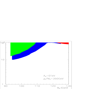
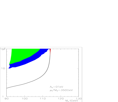
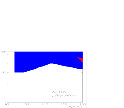
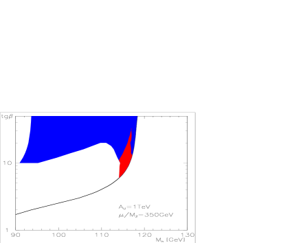
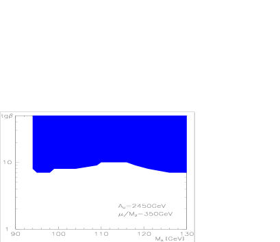
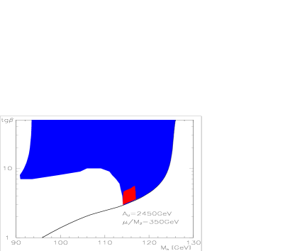
Figure 3: The allowed regions for $M_{A}$ [left] and $M_{h}$ [right] from LEP2 searches as a function of $\tan\beta$ (colored regions, or black, dark grey and light grey regions) in the case of maximal (bottom), typical (central) and no–mixing (up). The red (or dark grey) regions indicate where $114$ GeV$<M_{h}<117$ GeV and $\sin^{2}(\beta-\alpha)>0.9$ and the green (or light grey) regions indicate where $114$ GeV$<M_{H}<117$ GeV and $\cos^{2}(\beta-\alpha)>0.9$.

In these figures the colored (blue, green and red) areas correspond to the domains of the parameter space which are still allowed by the LEP2 searches. As can be seen, the allowed regions are different for the three scenarii of mixing in the stop sector.

In the no–mixing case, values $\tan\beta\raisebox{-3.69899pt}{~{}\shortstack{$<$ \\ [-0.07cm] $\sim$}}~{}10$ are excluded for any value of the pseudoscalar mass $M_{A}\raisebox{-3.69899pt}{~{}\shortstack{$>$ \\ [-0.07cm] $\sim$}}~{}90$ GeV. For a light $A$ boson, $M_{A}\raisebox{-3.69899pt}{~{}\shortstack{$<$ \\ [-0.07cm] $\sim$}}~{}100$ GeV and $\tan\beta\raisebox{-3.69899pt}{~{}\shortstack{$>$ \\ [-0.07cm] $\sim$}}~{}10$, the masses $M_{h}\sim M_{A}$ pass the bound (  $>$ [-0.07cm] $\sim$   91 GeV) from the Higgs pair production processs, while $H$ is light enough ($M_{H}\raisebox{-3.69899pt}{~{}\shortstack{$<$ \\ [-0.07cm] $\sim$}}~{}115$ GeV) to be probed in the Higgs–strahlung process. For increasing $M_{A}$, this situation holds only for larger $\tan\beta$: for instance, for $M_{A}\raisebox{-3.69899pt}{~{}\shortstack{$>$ \\ [-0.07cm] $\sim$}}~{}115$ GeV, one needs values $\tan\beta\raisebox{-3.69899pt}{~{}\shortstack{$>$ \\ [-0.07cm] $\sim$}}~{}40$ to cope with the experimental bounds [i.e. to make $H$ light enough to be produced]. In the typical mixing case, values $\tan\beta\raisebox{-3.69899pt}{~{}\shortstack{$<$ \\ [-0.07cm] $\sim$}}~{}10$ are excluded for $M_{A}$ close to 90 or 130 GeV. For intermediate $M_{A}$ values, one needs larger $\tan\beta$ values to evade the constraint from the Higgs–strahlung process since the $g_{hZZ}$ coupling is increasing while $M_{h}$ is relatively small, leading to a sizeable $\sigma(e^{+}e^{-}\to hZ)$. [Note that here, there is a strong interplay between the variation of $\sin^{2}(\beta-\alpha)$ and $M_{h}$ in the phase space in $\sigma(e^{+}e^{-}\to hZ)$, which explains the bump around $M_{A}\sim 115$ GeV.] For large $M_{A}$, $\tan\beta$ values close to 5 are still allowed since $M_{h}$ can be larger than 114 GeV. Finally, in the maximal mixing case, values $\tan\beta\raisebox{-3.69899pt}{~{}\shortstack{$>$ \\ [-0.07cm] $\sim$}}~{}7$ are excluded for 90 GeV $\raisebox{-3.69899pt}{~{}\shortstack{$<$ \\ [-0.07cm] $\sim$}}~{}M_{A}\raisebox{-3.69899pt}{~{}\shortstack{$<$ \\ [-0.07cm] $\sim$}}~{}130$ GeV. However, for large $M_{A}$, only values $\tan\beta\raisebox{-3.69899pt}{~{}\shortstack{$>$ \\ [-0.07cm] $\sim$}}~{}3$ are excluded since here, the large stop mixing increases the maximal value of $M_{h}$ to the level where it exceeds the discovery limit, $M_{h}\raisebox{-3.69899pt}{~{}\shortstack{$>$ \\ [-0.07cm] $\sim$}}~{}114$ GeV.

We turn now to the implications of the $2.1\sigma$ evidence for a SM–like Higgs boson with a mass $M_{\Phi_{H}}=115.6$ GeV, seen by the LEP collaborations in the Higgs–strahlung process [12]. In view of the theoretical and experimental uncertainties, this result will be interpreted as favoring the mass range $114\ {\rm GeV}\raisebox{-3.69899pt}{~{}\shortstack{$<$ \\ [-0.07cm] $\sim$}}~{}M_{\Phi_{H}}\raisebox{-3.69899pt}{~{}\shortstack{$<$ \\ [-0.07cm] $\sim$}}~{}117\ {\rm GeV}$. Furthermore, since this Higgs boson should be almost SM–like, we will impose the constraint $g^{2}_{ZZ\Phi_{H}}/g_{ZZH^{0}}^{2}\geq 0.9$ so that the cross section for the Higgs–strahlung process, $\sigma(e^{+}e^{-}\to\Phi_{H}Z)$, is maximized. Of course, at the same time [and in particular in the case where the “observed” Higgs boson is $H$] the experimental constraints from the pair production process, $M_{A},M_{h}\raisebox{-3.69899pt}{~{}\shortstack{$>$ \\ [-0.07cm] $\sim$}}~{}91$ GeV, should be taken into account.

The green areas show the regions where the “observed” Higgs boson is the heavier CP–even $H$ particle. This occurs only for no mixing with values $\tan\beta\raisebox{-3.69899pt}{~{}\shortstack{$>$ \\ [-0.07cm] $\sim$}}~{}15$ and $M_{A}\raisebox{-3.69899pt}{~{}\shortstack{$<$ \\ [-0.07cm] $\sim$}}~{}110$ GeV. In this case, $M_{H}\sim 115$ GeV and has SM–like couplings, while $M_{h}$ is still larger than 91 GeV. For large stop mixing, the $H$ boson is always heavier than 117 GeV and cannot be observed. The red areas correspond to the regions where the “observed” Higgs boson is in turn the lighter $h$ particle, while $M_{H}$ is heavier than 117 GeV. These regions are larger for the typical mixing scenario: in the no–mixing case, it is unlikely that the $h$ boson mass exceeds 114 GeV except for very large $\tan\beta$, while in the maximal mixing scenario, the $h$ boson is usually heavier than 117 GeV, except for very low $\tan\beta$.

Finally, let us briefly discuss the constraints on the intense–coupling scenario from the Higgs boson searches at the Tevatron. The first important constraint is coming from decays of the top quarks into $b$–quarks and charged Higgs bosons, $t\to bH^{+}$. For $\tan\beta$ values around unity [which are ruled out as discussed above] and for large values of $\tan\beta$, the $H^{-}t\bar{b}$ coupling, $g_{H^{-}tb}\propto m_{t}/\tan\beta+m_{b}\tan\beta$, is very strong. The branching ratio BR($t\to bH^{+}$) becomes then comparable and even larger than the branching ratio of the standard mode, $t\to bW^{+}$, which allows the detection of top quarks at the Tevatron. A search for this top decay mode, with the $H^{-}$ boson decaying into $\tau\nu_{\tau}$ final states, by the CDF and D0 Collaborations [29] allows to place stringent limits on the value of $\tan\beta$ for charged Higgs boson masses below $\sim 150$ GeV: for $M_{H^{\pm}}\simeq 120$ GeV [i.e. $M_{A}\simeq 90$ GeV] one has $\tan\beta\raisebox{-3.69899pt}{~{}\shortstack{$<$ \\ [-0.07cm] $\sim$}}~{}50$–60, while the bound becomes very weak for $M_{H^{\pm}}\simeq 150$ GeV [i.e $M_{A}\simeq 130$ GeV] where one has $\tan\beta\raisebox{-3.69899pt}{~{}\shortstack{$<$ \\ [-0.07cm] $\sim$}}~{}100$ [i.e. beyond the limit where the $b$–quark Yukawa coupling is perturbative].

Furthermore, constraints on the MSSM Higgs sector at the Tevatron can be derived [30] by exploiting the data on $\tau^{+}\tau^{-}+$ 2 jets used by the CDF Collaboration [31] to place limits on third generation leptoquarks. Indeed, in the associated production of the pseudoscalar $A$ boson with $b\bar{b}$ pairs, $pp\to q\bar{q}/gg\to b\bar{b}A$, with the $A$ boson decaying into $\tau^{+}\tau^{-}$ final states, the cross section is proportional to $\tan^{2}\beta$ and can be very large for $\tan\beta\gg 1$. In addition, since in this regime, one of the CP–even Higgs bosons is always degenerate in mass with the $A$ boson and has couplings to $b\bar{b}$ [and $\tau^{+}\tau^{-}$] pairs which are also proportional to $\tan\beta$, the rate for $b\bar{b}\tau^{+}\tau^{-}$ final states due to Higgs bosons in this type of process is multiplied by a factor 2. Since there is no evidence for non–SM contributions in this final state as analyzed by the CDF Collaboration, one can place bounds in the plane spanned by $\tan\beta$ and $M_{A}$. The upper bound is $\tan\beta\raisebox{-3.69899pt}{~{}\shortstack{$<$ \\ [-0.07cm] $\sim$}}~{}80$ for $M_{A}\raisebox{-3.69899pt}{~{}\shortstack{$>$ \\ [-0.07cm] $\sim$}}~{}90$ GeV, and is weaker for higher values of $M_{A}$, $\tan\beta\raisebox{-3.69899pt}{~{}\shortstack{$<$ \\ [-0.07cm] $\sim$}}~{}100$ for $M_{A}\sim 130$ GeV [30]. Therefore, this constraint is less severe than the one due to top decays into charged Higgs bosons [29].

There are two other processes for MSSM Higgs boson production which could be relevant at the Tevatron as will be discussed later. The gluon–gluon fusion mechanism, $gg\to\Phi$ with $\Phi\equiv h,H$ or $A$, can have large cross sections in particular for large $\tan\beta$ values, but the backgrounds in the main decay channel $\Phi\to b\bar{b}$ are too large while for the cleaner $\gamma\gamma$ decays, $\sigma\times{\rm BR}(\Phi\to\gamma\gamma)$ is too small. The associated production of the CP–even Higgs bosons $h$ or $H$ with a $W$ or $Z$ boson, has cross sections which are too small, in particular if the gauge bosons are required to decay leptonically. These processes will therefore be useful only when an integrated luminosity of a few femtobarn will be accumulated, i.e. only at the Run II of the machine [see section 5].

To summarize, the constraints on the Higgs sector from Tevatron data are not very strong and values of $\tan\beta$ slightly above $\tan\beta\sim 50$ [and below] are still allowed experimentally.

3.2 Indirect constraints from precision data

Indirect constraints on the parameters of the MSSM Higgs sector, in particular on $M_{A}$ and $\tan\beta$, come from the high–precision data: the measurements of the $\rho$ parameter from $M_{W}$ and $\sin^{2}\theta_{W}$, the decays $Z\to b\bar{b}$, the muon anomalous magnetic moment $(g_{\mu}-2)$ and the radiative decay $b\to s\gamma$. In discussing these constraints, we will neglect the contributions of the SUSY particles which are assumed to be heavy [$\mu=M_{2}=350$ GeV and $M_{S}=1$ TeV with $A_{t}=\sqrt{6}M_{S}$]. For an analysis of these SUSY contributions in a constrained MSSM, see Ref. [17] for instance. For completeness, we will also give the analytical expressions of the Higgs boson loop contributions to the observables in the intense–coupling regime.

a) The $\rho$ parameter

Loop contributions of the MSSM Higgs bosons can alter the values of the electroweak observables which have been precisely measured at LEP1, the SLC and the Tevatron [20, 21]. The dominant contributions to the weak observables, in particular the $W$ boson mass and the effective mixing angle $s_{W}^{2}\equiv\sin^{2}\theta_{W}$, enter via a deviation from unity of the $\rho$ parameter which, in terms of $W$ and $Z$ boson self–energies at zero momentum transfer, is defined by $\rho=(1-\Delta\rho)^{-1}$ with $\Delta\rho=\Pi_{ZZ}(0)/M_{Z}^{2}-\Pi_{WW}(0)/M_{W}^{2}$. Precision measurements constrain the contribution of New Physics to be $\Delta\rho^{\rm NP}\raisebox{-3.69899pt}{~{}\shortstack{$<$ \\ [-0.07cm] $\sim$}}~{}1.1\cdot 10^{-3}$ at the $1\sigma$ level [20].

In the intense-coupling regime, the contributions of the MSSM Higgs sector to the $\rho$ parameter is given by [note that the same expression holds exactly in the decoupling regime]:

$$\Delta\rho^{\rm Higgs}=-\frac{G_{F}M_{W}^{2}}{8\sqrt{2}\pi^{2}}\bigg{[}3f_{1}\bigg{(}\frac{M_{C}^{2}}{M_{Z}^{2}}\bigg{)}+2f_{2}\bigg{(}\frac{M_{H^{\pm}}^{2}}{M_{W}^{2}},\frac{M_{A}^{2}}{M_{W}^{2}}\bigg{)}\bigg{]}$$ (32)

with the two functions $f_{1}$ and $f_{2}$ given by [32]

$$f_{1}(x)=x\left[\frac{\ln c_{W}^{2}-\ln x}{c_{W}^{2}-x}+\frac{\ln x}{c_{W}^{2}(1-x)}\right]\ \ ,\ f_{2}(x_{1},x_{2})=\frac{x_{1}x_{2}}{x_{1}-x_{2}}\ln\frac{x_{2}}{x_{1}}+\frac{1}{2}(x_{1}+x_{2})$$ (33)

with $c_{W}^{2}=1-s_{W}^{2}$. The first contribution, $\Delta\rho^{\rm Higgs}_{\rm SM}=-3G_{F}M_{W}^{2}/(8\sqrt{2}\pi^{2})f_{1}(M_{C}^{2}/M_{Z}^{2})$, is simply the one of the SM Higgs boson with a mass $M_{H^{0}}=M_{C}$, which is close to the Higgs mass, ${\cal O}(100$ GeV), favored by the global fits of the electroweak data [21]. The second contribution, proportional to $f_{2}$, is the genuine MSSM contribution. The contribution of loops involving CP–even and CP–odd Higgs boson, $\sim-f_{2}(M_{A}^{2}/M_{W}^{2},M_{A}^{2}/M_{W}^{2})$ in the bracket, vanishes since $f_{2}(x,x)=0$. In fact, only loops which involve particles which have a large mass splitting contribute significantly to $\Delta\rho$. This is the reason why the genuine MSSM contribution, $\Delta\rho^{\rm Higgs}_{\rm non-SM}=-G_{F}M_{W}^{2}/(4\sqrt{2}\pi^{2})f_{2}(M_{H^{\pm}}^{2}/M_{W}^{2},M_{A}^{2}/M_{W}^{2})$, shown in Table 2, is always extremely small: the mass difference between the $H^{\pm}$ and $A$ bosons is not large enough. In turn, the SM–like Higgs contribution has a size which is comparable to the experimental error for $M_{H^{0}}=M_{C}\sim 127$ GeV [we use $\tan\beta=50$].

$M_{A}~{}[{\rm GeV}]$	90	110	130
$\Delta^{\rm Higgs}_{\rm non-SM}$	$-0.53\cdot 10^{-4}$	$-0.38\cdot 10^{-4}$	$-0.28\cdot 10^{-4}$
$\Delta^{\rm Higgs}_{\rm SM}$	$4.7\cdot 10^{-4}$	$4.7\cdot 10^{-4}$	$4.7\cdot 10^{-4}$

Table 2: The genuine and the SM–like contributions of the MSSM Higgs sector to the $\rho$ parameter in the intense–coupling regime with $\tan\beta=50$.

b) The g–2 of the muon

The precise measurement of the anomalous magnetic moment of the muon recently performed at BNL, $a_{\mu}\equiv g_{\mu}-2=11659202(20)\cdot 10^{-10}$ [23] where we have added the statistical and systematical errors, can provide very stringent tests of models of New Physics. In the MSSM, the Higgs sector will contribute to $a_{\mu}$ through loops involving the neutral Higgs bosons $h,H$ and $A$ with muons and loops involving the charged Higgs bosons $H^{\pm}$ with neutrinos. The contributions are sizeable only for large values of $\tan\beta$ for which the $\Phi\mu^{+}\mu^{-}$ and $H^{+}\mu\nu_{\mu}$ couplings are enhanced; for a recent analysis see Ref. [33].

Taking into account only the leading, $\propto\tan^{2}\beta$, contributions [i.e. neglecting the contribution of the SM–like CP–even Higgs boson $\Phi_{H}$] and working in the intense–coupling regime, one obtains for the MSSM Higgs sector contribution to $a_{\mu}$ [again, the expression holds also in the decoupling limit in this approximation]

$$a_{\mu}^{\rm Higgs}\simeq\frac{G_{F}m_{\mu}^{2}}{24\pi^{2}\sqrt{2}}\tan^{2}\beta\bigg{[}4\frac{m_{\mu}^{2}}{M_{A}^{2}}-\frac{m_{\mu}^{2}}{M_{H^{\pm}}^{2}}\bigg{]}$$ (34)

This contribution is given in Table 3 for $\tan\beta=50$ for $M_{A}=90,110$ and 130 GeV, and one can see that it is far too small compared to the experimental error. [Here, the approximated result which is displayed, is about 10 to 20 % smaller or larger than the exact result].

$M_{A}~{}[{\rm GeV}]$	90	110	130
$a_{\mu}^{\rm Higgs}$	$4.5\cdot 10^{-12}$	$2.9\cdot 10^{-12}$	$2.0\cdot 10^{-12}$

Table 3: Contribution of the MSSM Higgs sector to $a_{\mu}$ for $\tan\beta=50$.

c) The Zbb vertex

An observable where the MSSM Higgs sector can have sizeable effects is the $Z$ boson decay into $b\bar{b}$ final states. The neutral Higgs particles $h,H,A$ as well as the charged $H^{\pm}$ bosons can be exchanged in the $Zb\bar{b}$ vertex [34] and for large values of $\tan\beta$, for which the Higgs boson couplings to $b$ quarks are strongly enhanced, they can alter significantly the values of the partial decay width $\Gamma(Z\to b\bar{b})$ [or equivalently the ratio $R_{b}=\Gamma(Z\to b\bar{b})/\Gamma(Z\to{\rm hadrons})$ which is measured with a better accuracy] and the forward–backward asymmetry $A_{FB}^{b}$ [or the polarization asymmetry $A^{b}_{LR}$]. In terms of the left– and right–handed $Zf\bar{f}$ couplings, $g_{L/R}^{f}=I_{f}^{3}-e_{f}s_{W}^{2}$, and neglecting the $b$–quark mass for simplicity, they are given by:

$$\Gamma(Z\to b\bar{b})\simeq\frac{G_{F}M_{Z}^{3}}{\sqrt{2}\pi}[(g_{L}^{b})^{2}+(g_{R}^{b})^{2}]\ \ ,\ \ A_{FB}^{b}\simeq\frac{3}{4}\frac{(g_{L}^{e})^{2}-(g_{R}^{e})^{2}}{(g_{L}^{e})^{2}+(g_{R}^{e})^{2}}\frac{(g_{L}^{b})^{2}-(g_{R}^{b})^{2}}{(g_{L}^{b})^{2}+(g_{R}^{b})^{2}}$$ (35)

In the limit $\tan\beta\gg 1$, the MSSM neutral (N) and charged (C) Higgs boson contributions to the left– and right–handed bottom quark couplings are given by

$$\hskip 56.9055pt\delta g_{R/L}^{b}=\delta g_{R/L}^{b}|_{N}+\delta g_{R/L}^{b}|_{C}$$

$$\delta g_{R/L}^{b}|_{N} = \mp\bigg{(}\frac{gm_{b}\tan\beta}{\sqrt{2}M_{W}}\bigg{)}^{2}\bigg{[}C_{2}(m_{b},M_{A},M_{A})\pm g_{L/R}^{b}C_{1}(M_{A},m_{b},m_{b})\bigg{]}$$

$$\delta g_{R}^{b}|_{C} = -\bigg{(}\frac{gm_{b}\tan\beta}{\sqrt{2}M_{W}}\bigg{)}^{2}\bigg{[}\bigg{(}2s_{W}^{2}-1\bigg{)}C_{2}(m_{t},M_{H^{\pm}},M_{H^{\pm}})+g_{L}^{t}C_{1}(M_{H^{\pm}},m_{t},m_{t})$$ (36)

$$-g_{R}^{t}C_{0}(M_{H^{\pm}},m_{t},m_{t})\bigg{]}\ \ \ ,\ \ \ \delta g_{L}^{b}|_{C}=0$$

where the functions $C_{1,2}$ are given in terms of the Passarino–Veltman two– and three–point functions [the latter evaluated at $q^{2}=M_{Z}^{2}$ with $m_{b}\simeq 0$] by:

$$C_{2}(m_{1},m_{2},m_{2}) = C_{24}(m_{1},m_{2},m_{2})+\frac{1}{2}B_{1}(m_{1},m_{2})$$

$$C_{1}(m_{1},m_{2},m_{2}) = -\frac{1}{2}+2C_{24}(m_{1},m_{2},m_{2})-M_{Z}^{2}C_{23}(m_{1},m_{2},m_{2})+B_{1}(m_{1},m_{2})$$ (37)

The latest experimental values of $R_{b}$ and the forward backward asymmetry are [21]: $R_{b}=0.21653\pm 0.00069$ and $A_{FB}^{b}=0.099\pm 0.002$ [note that they deviate by, respectively, $+1.1\sigma$ and $-2.4\sigma$ from the predicted values in the SM]. This means that the virtual effects of the MSSM Higgs bosons should be, in relative size, of the order of $0.3\%$ in $R_{b}$ and $2\%$ in $A_{FB}^{b}$ to be detectable. This is far to be the case even for $\tan\beta$ values close to 50 and for $M_{A}\raisebox{-3.69899pt}{~{}\shortstack{$>$ \\ [-0.07cm] $\sim$}}~{}90$ GeV as can be seen from Table 4 where the approximate contributions [which are very close, at most a few percent, to the exact contributions] are displayed.

$M_{A}~{}[{\rm GeV}]$	90	110	130
$\Delta R_{b}/R_{b}$	$-5.0\cdot 10^{-4}$	$-7.5\cdot 10^{-4}$	$-8.3\cdot 10^{-4}$
$\Delta A_{\rm FB}^{b}/A_{\rm FB}^{b}$	$2.5\cdot 10^{-3}$	$2.5\cdot 10^{-3}$	$2.4\cdot 10^{-3}$

Table 4: Relative contribution of the MSSM Higgs sector to the two observables $R_{b}=\Gamma(Z\to b\bar{b})/\Gamma(Z\to{\rm hadrons})$ and $A_{\rm FB}^{b}$ for $\tan\beta=50$.

d) The $b\to s\gamma$ decay

Finally, in the radiative and flavor changing decay $b\to s\gamma$, in addition to the SM contribution built–up by $W$ boson and top quark loops, loops of charged Higgs bosons and top quarks can significantly contribute in the MSSM together with SUSY particle loops [35, 36]. Since SM and MSSM Higgs contributions appear at the same order of perturbation theory, the measurement of the inclusive branching ratio of the $B\rightarrow X_{s}\gamma$ given by the CLEO and Belle Collaborations [22] is a very powerful tool for constraining $\tan\beta$. We use the value [20]

$${\rm BR}(b\rightarrow s\gamma)=(3.37\pm 0.37\pm 0.34\pm 0.24^{+0.35}_{-0.16}\pm 0.38)\cdot 10^{-4}$$ (38)

where the errors are, respectively, the statistical error, the systematical error, the error from model dependence, the one due to the extrapolation from the data to take into account the full range of photon energies, and finally an estimate of the theory uncertainty. We allow the branching ratio to vary within the conservative range: $2\times 10^{-4}\leq{\rm BR}(b\rightarrow s\gamma)\leq 5\times 10^{-4}$.

For the calculation of the MSSM Higgs boson and SUSY particle contributions, we will use the most up–to–date determination of the $b\to s\gamma$ decay rate [36], where all known perturbative and non–perturbative effects are included. This includes all the possibly large contributions which can occur at NLO, such as terms $\propto\tan\beta$ [in particular in $m_{b}$], and/or terms containing logarithms of $M_{S}/M_{W}$. For the input parameters we will use the values given in Refs. [36], except for the cut–off on the photon energy, $E_{\gamma}>(1-\delta)m_{b}/2$ in the bremsstrahlung process $b\to s\gamma g$, which we fix to $\delta=0.9$. For the SUSY spectrum, we will work in the scenario discussed in section 2, i.e. a common squark mass $M_{S}=1$ TeV, the maximal mixing scenario $A_{t}=\sqrt{6}M_{S}$ and $A_{b}=1$ TeV, $\mu=M_{2}=350$ GeV.

$M_{A}~{}[{\rm GeV}]$	90	110	130
$\tan\beta=10$	$5.2\cdot 10^{-4}$	$5.0\cdot 10^{-4}$	$4.8\cdot 10^{-4}$
$\tan\beta=30$	$3.7\cdot 10^{-4}$	$3.5\cdot 10^{-4}$	$3.3\cdot 10^{-4}$
$\tan\beta=50$	$2.5\cdot 10^{-4}$	$2.3\cdot 10^{-4}$	$2.2\cdot 10^{-4}$

Table 5: BR($b\to s\gamma)$ in the MSSM for $\tan\beta=10,30,50$ and $M_{A}=90,110,130$ GeV.

Values of BR($b\to s\gamma$) in the MSSM are displayed for three choices of $\tan\beta$ and $M_{A}$ in Table 5, and one can see that they are in most cases within the allowed range $2\times 10^{-4}\leq{\rm BR}(b\rightarrow s\gamma)\leq 5\times 10^{-4}$. An exception is when $\tan\beta\sim 10$ and the $A$ boson is light, $M_{A}\raisebox{-3.69899pt}{~{}\shortstack{$<$ \\ [-0.07cm] $\sim$}}~{}110$ GeV, where the branching ratio slightly exceeds the maximal value; however, we have checked that for other values of the SUSY parameters a reasonable BR($b\to s\gamma)$ can be accommodated also in this case.

4. Branching fractions and total decay widths

The branching ratios and the total decay widths of the three neutral Higgs bosons [37], again evaluated with the program HDECAY with the set of input parameters discussed in section 2.4, are shown in Figs. 4–5 and 6 as functions of their masses for $M_{A}$ varying between 90 and 130 GeV, for two values of $\tan\beta$, 10 and 30.

In the case of the $A$ boson, the situation is rather simple since in the entire mass range shown, the pattern is the same: BR$(A\to\bar{b}b$) and BR($A\to\tau^{+}\tau^{-}$) are approximately 90% and 10%, respectively, while the gluonic branching fraction is slightly above $10^{-3}$ and BR$(A\to\mu^{+}\mu^{-})\sim 5\times 10^{-4}$. The branching ratios for the other decay modes, including the $A\to\gamma\gamma$ decay, are below the level of $10^{-5}$ for $\tan\beta\raisebox{-3.69899pt}{~{}\shortstack{$>$ \\ [-0.07cm] $\sim$}}~{}10$. This is due to the strong enhancement (suppression) of the $A$ couplings to isospin $-\frac{1}{2}(+\frac{1}{2})$ fermions [the $Agg$ coupling is mediated here mainly by the $b$–loop contribution]. Some of the final states which are important for larger $M_{A}$ values [such as the decay $A\to hZ$] are strongly suppressed by phase space in addition to the coupling suppression for large $\tan\beta$ values.

The pattern for the CP–even Higgs bosons is similar to that of the $A$ boson if their masses are close to $M_{A}$ and $\tan\beta\gg 1$. The exception is when $h$ and $H$ have masses very close to $M_{\rm C}$. In this limit, they are SM–like and decay into charm quarks and gluons with rates similar to the one for $\tau^{+}\tau^{-}$ [$\sim$ a few $\%$] and in the high mass range, $M_{H^{0}}\sim 125$ GeV, into $WW$ ($\sim 10\%$) and $ZZ$ (a few $\%$) pairs with one of the gauge bosons being virtual. However, this limit is not reached in practice, in particular for the lightest $h$ boson with $\tan\beta\raisebox{-3.69899pt}{~{}\shortstack{$<$ \\ [-0.07cm] $\sim$}}~{}50$.

Figure 4: The branching ratios of the neutral Higgs bosons $h,H$ and $A$ as a function of their masses for two values of $tan\beta=10$ (left panel) and 30 (right panel).

Figure 5: The branching ratios of the $h$ (left panel) and $H$ (right panel) bosons into $\gamma\gamma$, $gg$, $WW$, $\tau^{+}\tau^{-}$ final states as a function of $\tan\beta$ for $M_{A}=90,110,130$ GeV and $1$ TeV.

Indeed, as can be seen in Fig. 4, all decays of the $h$ boson other than $b\bar{b}$ and $\tau^{+}\tau^{-}$, are below the level of $10^{-3}$ for $\tan\beta=10$ and 30. In particular, we have BR($h\to\gamma\gamma)\raisebox{-3.69899pt}{~{}\shortstack{$<$ \\ [-0.07cm] $\sim$}}~{}10^{-4}$ and BR($h\to WW)\raisebox{-3.69899pt}{~{}\shortstack{$<$ \\ [-0.07cm] $\sim$}}~{}10^{-2}$ even for $M_{h}\sim 120$ GeV, i.e. at least one order of magnitude smaller than in the case of the SM Higgs boson. This is a consequence of the fact that the $h$ boson coupling to gauge bosons (and to up–type fermions) does not reach the SM limit while the couplings to $b$–quarks are still enhanced even for $M_{h}\sim M_{C}$; see Fig. 2 for the couplings. The $gg$ branching fraction is in turn almost constant, BR($h\to gg)\sim 10^{-3}$, since the $h\to gg$ decay width is dominantly mediated by the $b$–quark loop, but is suppressed by a factor of more than 20 compared to the SM case.

In the case of the heavier $H$ boson, the trend depends strongly on the value of $M_{A}$. For $M_{H}\raisebox{-3.69899pt}{~{}\shortstack{$>$ \\ [-0.07cm] $\sim$}}~{}125$ GeV, the branching ratios into the $\gamma\gamma,WW$ and $gg$ final states are much smaller than for the SM Higgs boson: for $\tan\beta$ values larger than $\sim 10$, they are at least two orders of magnitude smaller. Near the critical mass $M_{C}$, the branching fractions of the $H$ boson are in general closer to those of the SM Higgs particle. This is particularly true for $\tan\beta$ values smaller than $\sim 30$, where the branching fractions into $WW,gg$ and $\gamma\gamma$ ($\tau^{+}\tau^{-}$) final states are only slightly, less than a factor of two, smaller (larger) than for the SM Higgs particle. However, for larger values of $\tan\beta$ [not shown in Fig. 4a] a new feature occurs: the $H$ boson coupling to down–type fermions which is proportional to $\tan\beta$ [in the approximation discussed in Section 2, $g_{Hdd}\sim-f_{1}\tan\beta+f_{2}$ for $M_{A}<M_{C}$] becomes strongly suppressed and at some stage [close to $\tan\beta\sim f_{2}/f_{1}$ in our approximation] vanishes [note that this is not the case for up–type fermions and gauge bosons].

All these features can be seen more explicitly in Figs. 5, where the branching fractions of the $h$ and $H$ bosons into the $\tau^{+}\tau^{-},WW,gg$ and $\gamma\gamma$ final states are displayed as functions of $\tan\beta$ for three values of the $A$ mass in the intense–coupling regime $M_{A}=90,110$ and 130 GeV as well as in the decoupling limit with $M_{A}=1$ TeV. In particular, one can see that the branching fractions BR($H\to\tau^{+}\tau^{+})$, and hence BR$(H\to b\bar{b})$, drop at a given value of $\tan\beta$ [around $\tan\beta\sim 40$ for $M_{A}=90$ GeV and $\tan\beta\sim 50$ for $M_{A}=110$ GeV], therefore enhancing the rates of the $WW,gg$ and $\gamma\gamma$ decay modes. This is the only situation where the branching ratios for these decays are larger than in the case of the SM Higgs boson.

Finally, the total decay widths of the three neutral Higgs bosons are shown in Fig. 6. For $h$ and $H$ when they have masses close to $M_{C}$, the total decay widths are comparable to those of the SM Higgs boson, i.e. they are rather small. For $\tan\beta\raisebox{-3.69899pt}{~{}\shortstack{$>$ \\ [-0.07cm] $\sim$}}~{}10$, the $A$ boson and one of the CP–even Higgs bosons, i.e. $\Phi_{A}$, decay most of the time into $b$ quarks and $\tau$ leptons and the total decay widths are to a good approximation given by: $\Gamma_{\rm tot}\simeq G_{F}M_{A,\Phi_{A}}/(4\sqrt{2}\pi)\times\tan^{2}\beta(m_{\tau}^{2}+3\overline{m}_{b}^{2})$ and are therefore rather large. For $\tan\beta=50$ and $M_{A}\sim 130$ GeV, the total widths of the three neutral Higgs bosons are $\Gamma_{\rm tot}(A)\simeq 7.2$ GeV, $\Gamma_{\rm tot}(H)\simeq 6.96$ GeV (with $M_{H}=127.6$ GeV) and $\Gamma_{\rm tot}(h)\simeq 0.11$ GeV (with $M_{h}=123.9$ GeV).

Figure 6: The total decay widths of the neutral Higgs bosons $h,H$ and $A$ as a function of their masses for two values of $tan\beta=10,30$.

5. Production at Future Colliders

In this section, we present the production cross sections of the neutral MSSM Higgs bosons in the intense–coupling regime at future colliders. We will consider the case of the hadron colliders, the Tevatron Run II and the LHC, a future $e^{+}e^{-}$ linear collider with a c.m. energy of $\sqrt{s}=500$ GeV, in both the $e^{+}e^{-}$ and $\gamma\gamma$ modes [with the photons generated by back–scattering of laser light] and a $\mu^{+}\mu^{-}$ collider. In all cases, we will assume the values $\tan\beta=10$ and 30 and a heavy superparticle spectrum with the soft SUSY–breaking scalar masses set to $M_{S}=1$ TeV and trilinear couplings $A_{t}=2.6$ TeV, $A_{b}=1$ TeV [we recall the reader that here, the higgsino and gaugino masses are set to $\mu=M_{2}=1$ TeV]. Therefore only the standard processes, i.e. single or pair production and production in association with SM particles, will be considered. We will not discuss associated Higgs boson production with SUSY particles [39], Higgs boson production from the (cascade) decays of SUSY particles [40] or the effects of SUSY particle loops in the production processes [41].

5.1 Production at hadron colliders

The main production mechanisms of neutral MSSM Higgs bosons at hadron colliders are the following processes [see Ref. [42] and for recent reviews Refs. [2, 43, 44] for instance]:

$$\begin{array}[]{lccl}(a)&\ \ {\rm gluon-gluon~{}fusion}&\ \ gg\ \ \rightarrow&h,H,A\\ (b)&\ \ {\rm association~{}with~{}}\bar{b}b&gg,q\bar{q}\rightarrow&b\bar{b}+h,H,A\\ (c)&\ \ {\rm association~{}with~{}}\bar{t}t&gg,q\bar{q}\rightarrow&t\bar{t}+h,H,A\\ (d)&\ \ WW/ZZ~{}{\rm fusion}&\ \ VV\ \rightarrow&h,H\\ (e)&\ \ {\rm association~{}with}~{}W/Z&\ \ q\bar{q}\ \ \rightarrow&V+h,H\\ (f)&\ \ {\rm associated~{}pair~{}production}&\ \ q\bar{q}\ \ \rightarrow&A+h,H\end{array}$$

The single production of the pseudoscalar $A$ boson in the weak boson fusion processes or in association with massive gauge bosons, as well as the pair production of two CP–even Higgs bosons, do not occur at leading order because of CP–invariance. Higgs boson production in association with other SM particles has too small cross sections.

All the production cross sections are shown in Figs. 7–12 for the LHC with $\sqrt{s}=14$ TeV and for the upgraded Tevatron with $\sqrt{s}=2$ TeV. These cross sections have been obtained using the package CompHEP [45] [see Ref. [46] for details of the MSSM implementation in CompHEP by means of the LanHEP program], with the Higgs sector adapted from HDECAY for consistency with the discussion of the Higgs properties given previously. The parton densities are taken from the sets CTEQ5L and CTEQ5M1 [47] with the scale set at the Higgs boson mass. The choice of scale and parton density might lead to a 30% uncertainty in the production cross sections.

The next–to–leading order QCD corrections are taken into account in the $gg$ fusion processes where they are large, leading to an increase of the production cross sections by a factor of up to two [48]. For the other processes, the QCD radiative corrections are relatively smaller [49]: for the associated production with gauge bosons and associated Higgs pair production, the corrections [which can be inferred from the Drell–Yan $W/Z$ production] are at the level of $10\%$, while in the case of the vector boson fusion processes, they are at the level of $30\%$. For the associated production with heavy quarks, the NLO corrections are only available in the case of the production of the SM Higgs boson with $t\bar{t}$ pairs [50] where they alter the cross section by $\sim 20\%$ if the scale is chosen properly. To include these corrections and to obtain the corresponding $K$–factors, we have linked CompHEP with the programs HIGLU, HPAIR, HQQ, V2HV and VV2H [51] which have all these corrections incorporated.

Let us now briefly summarize the main features of these processes, relying for the experimental searches on the analyses performed by various collaborations [?–?].

a) Gluon–gluon fusion

This mechanism is mediated by top and bottom quark loops and is therefore sensitive to both the $b\bar{b}$ and $t\bar{t}$–Higgs Yukawa couplings, allowing for the measurement of these important parameters [in conjunction with other production processes with the same Higgs decay modes] if the uncertainties from parton densities and higher order QCD corrections are properly under control. In the large $\tan\beta$ regime, the $b$–loop contributions are dominant since they are enhanced by $\tan^{2}\beta$ factors. The top–quark loop gives a relatively important contribution only in the case of the SM–like CP–even Higgs boson $\Phi_{H}$ i.e. $h$ or $H$ for $M_{A}\geq M_{C}$ or $M_{A}\leq M_{C}$, respectively. The cross sections are not the same for the pseudoscalar $A$ boson and the CP–even Higgs boson $\Phi_{A}$ even for large $\tan\beta$ where the Higgs–$\bar{b}b$ Yukawa couplings are similar: this is due to the appearance of different loop induced Higgs–$gg$ form factors for CP–even and CP–odd particles. The cross sections for the production of the $A$ and $h$ boson decrease quickly for increasing $M_{A}$ [a factor $\sim 5$ for $M_{A}$ varying from 90 to 130 GeV]; the cross section for $H$ stays almost constant since $M_{H}$ does not vary too much in this range.

At the LHC, for $\tan\beta\sim 10$, the cross sections for the $A$ and $h$ bosons vary from ${\cal O}(150)$ pb for a low mass $A$ boson, $M_{A}\sim 90$ GeV, to ${\cal O}(30)$ pb for $M_{A}\sim 130$ GeV; the cross section for $H$ production stays at the level of 30 to 50 pb in this mass range. This leads to a huge number of events, ${\cal O}(10^{7})$ per year for an integrated luminosity of $\int{\cal L}\sim 100$ fb^-1 as expected in the high–luminosity option. For $\tan\beta\sim 30$, the cross sections are one order of magnitude larger for the $A$ and $\Phi_{A}$ bosons [while it stays roughly constant for the $\Phi_{H}$ boson] as a result of the increase of the Higgs–$b\bar{b}$ Yukawa coupling. At the Tevatron, the trend is practically the same as at the LHC [note that here, the initiated $q\bar{q}$ process plays a more important role than at high energies due to the reduced gluon luminosity] except that the cross section is $\sim 30$ times smaller. Nevertheless, with the integrated luminosity of $\int{\cal L}\sim 30$ fb^-1 expected at the end of the Run II option, this would lead to at least ${\cal O}(10^{4})$ Higgs bosons in each of the $gg\to A,\Phi_{A}$ processes.

Figure 7: Production cross sections at the LHC (upper panel) and at the Tevatron (lower panel) for the gluon-gluon fusion mechanism as functions of $M_{A}$ for $\tan\beta=10,30$.

Let us now discuss the signatures which would allow for the detection of these Higgs particles. In all cases, the $b\bar{b}$ final states cannot be used because of the huge QCD 2–jet background and the lack of a clean leptonic trigger. At the LHC, the final states which can be probed for the SM–like Higgs boson $\Phi_{H}$ would be in principle the $\Phi_{H}\to\gamma\gamma$ final state for which the branching ratio can be of order $10^{-3}$. However, this occurs only if $\Phi_{H}$ is pure SM–like which, in the scenario discussed in Fig. 5, occurs only for the $H$ boson for a rather light $A$ boson and moderate to large $\tan\beta$ values. This is exemplified in Table 6 where are shown the cross sections for $h,H$ and $A$ boson production in the $gg$ fusion mechanism times the Higgs decay branching ratio into $\gamma\gamma$ final states, relative to the SM case [with the SM Higgs boson having the same mass as the $h,H$ or $A$ boson]. In the case of $H$, only for large $\tan\beta$ and moderate $M_{A}$ values, the cross section times branching ratio exceeds the SM value [with a factor up to 3]. For the pseudoscalar $A$ boson, the very small $\gamma\gamma$ branching ratio is not compensated by the large cross section. Therefore, the ratio is much smaller than unity. In the case of the lighter $h$ boson, we are not yet in the decoupling limit even for $M_{A}\sim 130$ GeV and $\tan\beta\sim 50$, and the cross section times branching ratio $\sigma(gg\to h)\times{\rm BR}(h\to\gamma\gamma$) is at least two orders of magnitude smaller than in the SM.

Thus, there are situations where $\sigma(\Phi)\times{\rm BR}(\Phi\to\gamma\gamma$) is rather small for the three Higgs bosons $h,H$ and $A$ compared to the SM case, making this channel more difficult to use. In addition, for the $A$ and $\Phi_{A}$ particles, the total decay widths are much larger than in the SM, leading to broader signals and therefore a much larger $\gamma\gamma$ background. The $\Phi_{H}\to WW$ and $ZZ$ final states would be also very difficult to use since in our case $M_{\Phi_{H}}\sim 130$ GeV and the branching ratios are too small even for SM $\Phi_{H}VV$ couplings.

At the Tevatron, although very difficult, only the $\Phi_{H}\to\tau^{+}\tau^{-}$ channel might be used as preliminary studies seem to indicate [52]. The branching ratios for the $h,H$ and $A$ boson decays into $\tau^{+}\tau^{-}$ final states are always of the order of $10\%$ except in the “pathological” situations discussed in section 4, where the $H\tau^{+}\tau^{-}$ coupling is suppressed. For the $A$ and $\Phi_{A}$ bosons, the channels $A,\Phi_{A}\to\tau^{+}\tau^{-}$ can be used at the LHC in the high $\tan\beta$ regime, $\tan\beta\raisebox{-3.69899pt}{~{}\shortstack{$>$ \\ [-0.07cm] $\sim$}}~{}10$, where the cross sections are large enough. At the Tevatron, because of the smaller cross sections, this channel is expected to be more difficult, although the analyses mentioned previously give some hope.

$\ \tan\beta\$	$M_{A}$	$\frac{\sigma(A)\times{\rm BR}(\gamma\gamma)|_{\rm MSSM}}{\sigma(H^{0})\times{\rm BR}(\gamma\gamma)|_{\rm SM}}$	$M_{h}$	$\frac{\sigma(h)\times{\rm BR}(\gamma\gamma)|_{\rm MSSM}}{\sigma(H^{0})\times{\rm BR}(\gamma\gamma)|_{\rm SM}}$	$M_{H}$	$\frac{\sigma(H)\times{\rm BR}(\gamma\gamma)|_{\rm MSSM}}{\sigma(H^{0})\times{\rm BR}(\gamma\gamma)|_{\rm SM}}$
	90	$1.5\cdot 10^{-3}$	84.9	$7.5\cdot 10^{-3}$	125.1	$0.6$
10	110	$3.7\cdot 10^{-4}$	103.9	$5.6\cdot 10^{-3}$	126.8	$0.15$
	130	$1.4\cdot 10^{-4}$	117.1	$1.2\cdot 10^{-2}$	134.0	$1.4\cdot 10^{-2}$
	90	$1.8\cdot 10^{-2}$	85.9	$2.2\cdot 10^{-2}$	124.0	$1.9$
30	110	$5.0\cdot 10^{-3}$	106.6	$6.7\cdot 10^{-3}$	124.2	$0.36$
	130	$2.1\cdot 10^{-3}$	123.2	$1.2\cdot 10^{-2}$	128.0	$1.8\cdot 10^{-3}$
	90	$5.2\cdot 10^{-2}$	85.7	$5.6\cdot 10^{-2}$	124.3	$2.0$
50	110	$1.4\cdot 10^{-2}$	106.5	$1.5\cdot 10^{-2}$	124.4	$3.2$
	130	$6.2\cdot 10^{-3}$	124.3	$2.3\cdot 10^{-2}$	127.1	$4.3\cdot 10^{-3}$

Table 6: The ratios $\sigma(gg\to\Phi)\times{\rm BR}(\Phi\to\gamma\gamma)$ in the MSSM with $\Phi=h,H$ and $A$ relative to the SM case for a SM Higgs boson with the same mass, for three values of $\tan\beta=10,30$ and 50 and three values of the pseudoscalar boson mass $M_{A}=90,110$ and $130$ GeV.

b) Associated production with bottom quarks

In these processes, the production cross sections for the $A$ and $\Phi_{A}$ bosons are also strongly enhanced by $\tan^{2}\beta$ factors. The rates are similar to those in the $gg$ fusion processes, ${\cal O}(100)$ pb at the LHC and ${\cal O}(1)$ pb at the Tevatron for $M_{A}\sim 90$–100 GeV and $\tan\beta=10$, and are one order of magnitude larger for $\tan\beta=30$. They decrease more slowly with increasing Higgs boson mass than in the case of $gg$ fusion and the cross sections are closer in magnitude for the $A$ and $\Phi_{A}$ bosons [in fact, they must be equal for equal Yukawa couplings when the final state $b$–quark mass is neglected, i.e. in the “chiral” limit]. In turn the cross section for associated production of the SM–like $\Phi_{H}$ boson is much smaller due to a tiny (not enough enhanced) Yukawa coupling.

Figure 8: Production cross sections at the LHC (upper panel) and at the Tevatron (lower panel) for Higgs bosons in association with $b$ quarks as functions of $M_{A}$ for $\tan\beta=10,30$.

Because of the small number of events, the detection of the $\Phi_{H}$ boson in this process is practically hopeless. In turn, the detection of the $A$ and $\Phi_{A}$ bosons is more promising than in the $gg$ fusion process since we do not have to rely on decays into photons or massive gauge bosons which here, are absent or strongly suppressed. Indeed, the additional two $b$–quarks in the final state, which can be rather efficiently tagged using micro–vertex detectors, will reduce dramatically the QCD backgrounds [especially since the production cross sections can be very large] to the level where the final states $A,\Phi_{A}\to\tau^{+}\tau^{-}$ at the LHC and $A,\Phi_{A}\to\bar{b}b$ at the Tevatron could be easily detectable for $\tan\beta\raisebox{-3.69899pt}{~{}\shortstack{$>$ \\ [-0.07cm] $\sim$}}~{}10$.

c) Associated production with top quarks

Figure 9: Production cross sections at the LHC (upper panel) and at the Tevatron (lower panel) for Higgs bosons in association with top quarks as functions of $M_{A}$ for $\tan\beta=10,30$.

Here, the production cross sections are suppressed by the smaller phase space [in particular at the Tevatron] compared to the previous case and by the fact that the $t\bar{t}$–Higgs Yukawa coupling is not enhanced compared to the SM case. To the contrary, the cross sections are strongly suppressed by $\tan^{2}\beta$ factors for the production of the $A$ and $\Phi_{A}$ bosons. A reasonably large cross section is obtained for the production of the $\Phi_{H}$ boson, reaching the level of $\sim 0.3$ pb at the LHC and 2.5 fb at the Tevatron. In a large part of the parameter space we are concerned with, i.e. for 90 $\raisebox{-3.69899pt}{~{}\shortstack{$<$ \\ [-0.07cm] $\sim$}}~{}M_{A}\raisebox{-3.69899pt}{~{}\shortstack{$<$ \\ [-0.07cm] $\sim$}}~{}130$ GeV and $\tan\beta\raisebox{-3.69899pt}{~{}\shortstack{$>$ \\ [-0.07cm] $\sim$}}~{}10$ [even around the turning point $M_{A}\sim 125$ GeV], the sum of the cross sections for $h$ and $H$ production is comparable to the one in the SM, since the sum of the squared couplings $g_{ht\bar{t}}^{2}+g_{Ht\bar{t}}^{2}=1/\sin^{2}\beta\sim 1$ for $\tan\beta\raisebox{-3.69899pt}{~{}\shortstack{$>$ \\ [-0.07cm] $\sim$}}~{}10$ and the Higgs masses are comparable.

The detection of the $\Phi_{H}$ boson in this process is in principle possible either through its $\gamma\gamma$ or $\bar{b}b$ decay modes. In the $\gamma\gamma$ channel, the detection is however more difficult in general than in the SM, due to the reduced $\gamma\gamma$ branching ratio in most of the parameter space as discussed previously. The $\Phi_{H}\to\bar{b}b$ final state gives a more promising detection signal since the branching ratio is in general (slightly) larger than in the SM.

d) WW/ZZ fusion processes

Figure 10: Production cross sections at the LHC (upper panel) and at the Tevatron (lower panel) for the vector boson fusion mechanisms as functions of $M_{A}$ for $\tan\beta=10,30$.

Here the cross sections are two to three orders of magnitude smaller than in the $gg\to\Phi$ and $b\bar{b}\Phi$ processes. They only reach the level of $\sim 5$ pb at the LHC and $\sim 0.1$ pb at the Tevatron for a SM–like Higgs boson which has maximal coupling to gauge bosons. For the $\Phi_{A}$ boson, the rates are too small in particular for $\tan\beta\raisebox{-3.69899pt}{~{}\shortstack{$>$ \\ [-0.07cm] $\sim$}}~{}10$.

At the Tevatron, the cross sections are very small and this process is too difficult to be used. At the LHC, the decay into $\tau^{+}\tau^{-}$ final states would allow for the detection of the $\Phi_{H}$ particles, similarly as in the SM model, by taking advantage of the energetic quark jets in the forward and backward directions which allow for additional cuts to suppress the backgrounds. However, there are situations where both products $\sigma(VV\to h,H)\times{\rm BR}(h,H\to\tau^{+}\tau^{-})$ are suppressed compared to the SM case as shown in Table 7 for several values of $\tan\beta$ and $M_{A}$. This occurs for large $\tan\beta\raisebox{-3.69899pt}{~{}\shortstack{$>$ \\ [-0.07cm] $\sim$}}~{}30$ and small $M_{A}\sim 90$ GeV, where the ratio $\sigma(\Phi)\times{\rm BR}(\tau\tau)|_{\rm MSSM}/\sigma(H^{0})\times{\rm BR}(\tau\tau)|_{\rm SM}$ with $\Phi=h(H)$ is strongly (slightly) suppressed. For $\tan\beta\sim 10$ and $M_{A}\sim 130$ GeV, both ratios are slightly smaller than unity, 15% for $\Phi=h$ and 30% for $\Phi=H$, but in this case the sum of the ratios is larger than one. In addition, in the pathological regions where the $H$ boson couplings to $\tau$ leptons is suppressed [for instance $\tan\beta\sim 50$ and $M_{A}\sim 110$ GeV], one can have a very tiny cross section times branching ratio, since in this case, the lighter $h$ is $\Phi_{A}$ like and does not couple to vector bosons.

$\ \tan\beta\$	$M_{A}$	$M_{h}$	$\frac{\sigma(h)\times{\rm BR}(\tau\tau)|_{\rm MSSM}}{\sigma(H^{0})\times{\rm BR}(\tau\tau)|_{\rm SM}}$	$M_{H}$	$\frac{\sigma(H)\times{\rm BR}(\tau\tau)|_{\rm MSSM}}{\sigma(H^{0})\times{\rm BR}(\tau\tau)|_{\rm SM}}$
	90	84.9	$6.6\cdot 10^{-2}$	125.1	$1.16$
10	110	103.9	$0.2$	126.8	$1.24$
	130	117.1	$0.85$	134.0	$0.68$
	90	85.9	$3.1\cdot 10^{-3}$	124.0	$0.63$
30	110	106.6	$1.3\cdot 10^{-2}$	124.2	$1.32$
	130	123.2	$1.2$	128.0	$0.25$
	90	85.7	$1.2\cdot 10^{-4}$	124.3	$0.49$
50	110	106.5	$4.8\cdot 10^{-4}$	124.4	$6.3\cdot 10^{-4}$
	130	124.3	$1.4$	127.1	$2.3\cdot 10^{-2}$

Table 7: The ratios $\sigma(VV\to\Phi)\times{\rm BR}(\Phi\to\tau\tau)$ in the MSSM with $\Phi=h,H$ relative to the SM case for a SM Higgs boson $H^{0}$ with the same mass, for three values of $\tan\beta=10,30$ and 50 and three values of the pseudoscalar boson mass $M_{A}=90,110$ and 130 GeV.

e) Associated production with W/Z bosons

At the LHC, these associated production processes would allow for the measurement of the Higgs boson couplings to the massive gauge bosons [again in conjunction with other production and decay processes]. The cross sections for $W\Phi_{H}$ associated production are at the level of $\sim 1.5$ pb at the LHC and $\sim 150$ fb at the Tevatron. They are of course slightly smaller than for a SM Higgs boson with the same mass. The cross sections for $Z\Phi_{H}$ associated production are smaller by approximately a factor of 2. Because of the fact that the gauge bosons are tagged through their leptonic decays, $W$–boson final states are much more interesting since their leptonic branching fractions are larger.

Figure 11: Cross sections at the LHC (upper panel) and at the Tevatron (lower panel) for the associated Higgs production with gauge bosons as functions of $M_{A}$ for $\tan\beta=10,30$.

At the Tevatron, these processes are the most promising ones to detect a SM–like Higgs boson at the Tevatron [44]. Since the branching fraction for the decay mode $\Phi_{H}\to b\bar{b}$ is always larger than in the SM, except in the pathological cases discussed above, the situation is rather favorable for the process $p\bar{p}\to W\Phi_{H}$ if the cross section is only slightly suppressed compared to the SM case. In fact, the ratio of cross sections times branching ratios into $b\bar{b}$, $\sigma(\Phi V)\times{\rm BR}(bb)$, compared to the SM case, is the same as the one for the vector boson fusion with the Higgs bosons decaying into $\tau^{+}\tau^{-}$ final states [since the cross sections are governed by the same $\Phi VV$ couplings and the ratio BR$(\Phi\to\tau^{+}\tau^{-})$/BR($\Phi\to b\bar{b})\sim m_{\tau}^{2}/3\overline{m}_{b}^{2}$ is constant]. Therefore, the situation is similar to that of the previous case (d) and the possibility that the cross sections times branching ratios are small for both $h$ and $H$ can occur.

The situation is more complicated at the LHC if the Higgs bosons have to be detected through their $\gamma\gamma$ decay modes, since the $\gamma\gamma$ branching ratios are in general smaller than in the SM and the total decay widths of the states are much larger, as discussed previously [especially since already in the SM, the significance for this process is rather low].

f) Associated pair production

Figure 12: Cross sections at the LHC (upper panel) and at the Tevatron (lower panel) for the associated Higgs boson pair production processes as functions of $M_{A}$ for $\tan\beta=10,30$.

The associated pair production of CP–even and CP–odd Higgs bosons through the $s$–channel exchange of a $Z$ boson has the lowest production cross section of all processes. The event rates are reasonable only for the $q\bar{q}\to Ah$ process in the lower mass range of the $A$ boson, where the cross section is above the level of 0.1 pb at the LHC and 10 fb at the Tevatron. In this range, both the $A$ and $\Phi_{A}$ bosons will decay into $b\bar{b}$ pairs so that the most advantageous final state [in terms of production rate] to consider is 4 $b$–jets, the rate for the $b\bar{b}\tau^{+}\tau^{-}$ final state being an order of magnitude lower.

To our knowledge, the detection of MSSM Higgs bosons at the Tevatron and the LHC in these processes has not been subject to experimental scrutinity. This is probably due to the difficulty of extracting such a small 4 $b$–jet signal from the background. However, it might be interesting to look at such final states, not only for this particular process but also in Higgs boson pair production in higher order processes where the trilinear Higgs boson couplings are involved as will be discussed below.

g) Pair production of Higgs bosons in higher order processes

Pair production of Higgs bosons in the $gg$ fusion occurs through triangle loop diagrams mediated by top and bottom quark exchange where a Higgs boson is produced (off–shell in our case) and splits into two Higgs particles, and box diagrams where the two Higgs particles are radiated from the internal top and bottom quark lines. These processes are of higher order in the electroweak coupling and therefore have small cross sections [53, 54] compared to the dominant processes discussed previously. However, they are interesting to consider since they involve the trilinear Higgs boson couplings [in the vertex diagrams where a virtual Higgs bosons splits into two Higgs bosons], the measurement of which is important in order to reconstruct the MSSM Higgs potential. We will thus discuss shortly these processes at the LHC and at the Tevatron. Additional processes such as the double Higgs production in association with $W$ and $Z$ bosons, the double Higgs production in the $WW/ZZ$ fusion processes and the triple Higgs production in $q\bar{q}$ collisions, can also give access to the trilinear Higgs boson couplings; however, the cross sections are in general smaller than in the $gg$ fusion mechanism and we will not discuss them here [54].

The production cross sections for the double production of Higgs bosons of any kind,

$$(g)\ \ gg\to hh,Hh,HH,HA,hA,AA$$

are shown in Figs. 13 for the LHC and Tevatron energies [for the latter case, only for $\tan\beta=30$ and for those which are large enough]. At the LHC, the cross sections are in general well below the level of 0.1 pb. They can reach the picobarn level only for very large $\tan\beta$ values, $\tan\beta\raisebox{-3.69899pt}{~{}\shortstack{$>$ \\ [-0.07cm] $\sim$}}~{}30$, small $A$ boson mass and only for the channels where only $A$ or $h$ are involved, $gg\to hh$ and $AA$. In this regime, the Higgs bosons will decay predominantly into $b\bar{b}$ pairs so that the final state will also be 4 $b$–quarks, as is the case for associated Higgs boson pair production which, as discussed previously, has similar cross sections in the same $M_{A}$ range and is a difficult process to detect experimentally. In fact, when the cross sections are sizable enough, the main contribution is due to the diagrams where both Higgs bosons are emitted from the internal $b$–quark lines when the Higgs–$\bar{b}b$ Yukawa coupling is strongly enhanced. The triangle diagram which is sensitive to the trilinear Higgs boson coupling gives only a small contribution, and these couplings can thus not be probed. At the Tevatron, the cross sections are two orders of magnitude smaller than at the LHC because of the reduced phase space and the much lower $gg$ luminosity. They are maximal for the $gg\to hh$ and $AA$ processes where they reach the 10 fb level in the same regime as at the LHC, i.e. for small $M_{A}$ and large $\tan\beta$ where the contribution from Higgs emission from the internal $b$–quarks is enhanced and the trilinear couplings play a minor role.

Figure 13: Production cross sections at the LHC (full lines) and the Tevatron (dashed lines) for the double Higgs boson production processes $gg\to\Phi_{1}\Phi_{2}$ as functions of $M_{A}$ for $\tan\beta=10$ (left panel) and $\tan\beta=30$ (right panel).

5.2 Production at electron–positron colliders

At $e^{+}e^{-}$ linear colliders operating in the 500 GeV energy range, the main production mechanisms for MSSM neutral Higgs particles in the $e^{+}e^{-}$ option are [2, 55, 56]

$$\begin{array}[]{lccl}(a)&\ \ {\rm bremsstrahlung\ process}&\ \ e^{+}e^{-}&\rightarrow(Z^{*})\rightarrow Z+h,H\\ &\ \ {\rm associated\ production\ process}&\ \ e^{+}e^{-}&\rightarrow(Z^{*})\rightarrow A+h,H\\ (b)&\ \ WW\ {\rm fusion\ process}&\ \ e^{+}e^{-}&\rightarrow\bar{\nu}_{e}\ \nu_{e}\ W^{*}W^{*}\rightarrow\bar{\nu}_{e}\nu_{e}\ +h,H\\ &\ \ ZZ\ {\rm fusion\ process}&\ \ e^{+}e^{-}&\rightarrow e^{+}e^{-}Z^{*}Z^{*}\rightarrow e^{+}e^{-}+h,H\\ (c)&\ \ {\rm radiation~{}off~{}top~{}quarks}&\ \ e^{+}e^{-}&\rightarrow(\gamma^{*},Z^{*})\rightarrow t\bar{t}+h,H,A\\ &\ \ {\rm radiation~{}off~{}bottom~{}quarks}&\ \ e^{+}e^{-}&\rightarrow(\gamma^{*},Z^{*})\rightarrow b\bar{b}+h,H,A\end{array}$$

Again, the associated production of the pseudoscalar $A$ and $Z$ bosons, the single production of the $A$ boson in the fusion processes as well as the pair production of two CP–even or two CP–odd Higgs particles can only occur at higher orders [57] because of CP invariance. The production cross sections are shown in Figs. 14–16 as functions of the pseudoscalar $A$ boson mass for a center of mass energy $\sqrt{s}=500$ GeV and for two values $\tan\beta=10$ and 30. Let us briefly discuss the cross sections of these various processes.

a) Higgs–strahlung and Higgs pair production

These are the most interesting processes in this context. The cross sections for the bremsstrahlung and the pair production processes as well as the cross sections for the production of the $h$ and $H$ bosons are mutually complementary, coming either with a coefficient $\sin^{2}(\beta-\alpha)$ or $\cos^{2}(\beta-\alpha)$. The cross section for $hZ$ production is large for large values of $M_{h}$, i.e. close to the decoupling limit. By contrast, the cross section for $HZ$ production is large for a light $A$ boson implying a light $H$ boson with a large coupling to $Z$ bosons. For the associated production, the situation is opposite: the cross section for $Ah$ is large for a light $h$ boson whereas $AH$ production is preferred in the complementary region.

Figure 14: Total cross sections at a 500 GeV $e^{+}e^{-}$ collider in the Higgs strahlung and associated Higgs production processes as functions of $M_{A}$ for $\tan\beta=10,30$.

At $\sqrt{s}=500$ GeV, the sums of the cross sections $\sigma(e^{+}e^{-}\to hZ+HZ)$ and $\sigma(e^{+}e^{-}\to hA+HA)$ are, respectively, $\sim 60$ and $\sim 40$ fb in the entire $M_{A}$ range. This means that with the integrated luminosity, $\int{\cal L}\sim 500$ fb^-1, expected at the TESLA machine for instance, approximately 30.000 and 20.000 events per year can be collected in these two channels, respectively. In the Higgs–strahlung process, the signals consist mostly of a $Z$ boson and a $b\bar{b}$ pair, which is easy to separate from the main background, $e^{+}e^{-}\rightarrow ZZ$ [for $M_{h}\simeq M_{Z}$, efficient $b$ detection is needed]. For the associated Higgs boson production, the signals consist mostly of four $b$ quarks in the final state, requiring efficient $b$–quark tagging.

b) Vector boson fusion processes

The trend for the production cross sections of the $h$ and $H$ boson in vector boson fusion is the same as in the Higgs–strahlung processes since both are proportional to the square of the Higgs–$VV$ couplings. At $\sqrt{s}\sim 500$ GeV, the production rate for the $WW$ fusion mechanism is slightly larger than the one for the Higgs–strahlung process, $\sigma(e^{+}e^{-}\to H\nu\bar{\nu}+h\nu\bar{\nu})\sim 80$ fb compared to $\sigma(e^{+}e^{-}\to hZ+HZ)\sim 60$ fb. A large sample of events is therefore expected, 40.000 events per year with the luminosity $\int{\cal L}\sim 500$ fb^-1, with a signature consisting mainly of a $b\bar{b}$ or a $\tau^{+}\tau^{-}$ pair and missing energy. The cross sections for the $ZZ$ fusion processes are one order of magnitude smaller than the ones for $WW$ fusion, a consequence of the smaller neutral current couplings compared to charged current couplings. The signal is however cleaner due the additional $e^{+}e^{-}$ pair in the final state.

Note that for other c.m. energies, the Higgs–strahlung cross section, which scales as $1/s$, dominates at lower energies while the $WW$ fusion mechanism which has a cross section rising like $\log(s/M_{H}^{2})$ dominates at higher energies.

Figure 15: Production cross sections at a 500 GeV $e^{+}e^{-}$ collider in the vector boson fusion processes as functions of $M_{A}$ for $\tan\beta=10,30$.

c) Higgs production with heavy quarks

For Higgs boson production in association with top quarks, the production cross sections are strongly suppressed for the $A$ and $\Phi_{A}$ boson for $\tan\beta\raisebox{-3.69899pt}{~{}\shortstack{$>$ \\ [-0.07cm] $\sim$}}~{}10$ and are sizeable only for the $\Phi_{H}$ boson which has almost SM–like couplings to the top quarks. Even in this case, they are however very small, barely exceeding the level of 0.2 fb. This is due to the fact that at $\sqrt{s}=500$ GeV, there is only a little amount of phase–space [$\sim 50$ GeV] available for this process. At higher energies, e.g. $\sqrt{s}=800$ GeV, the cross sections can exceed the level of $\sim 1$ fb which would allow for the measurement of the $\Phi_{H}t\bar{t}$ couplings since most of the cross section is coming from the Higgs boson radiation off the top quarks.

In the case of Higgs boson production in association with bottom quarks, we have taken into account only the gauge invariant contribution coming from Higgs boson radiation off the $b$–quark lines since a much larger contribution would come from the associated production process $e^{+}e^{-}\to Ah$ or $AH$, with one of the Higgs boson decaying into $b\bar{b}$, or from the Higgs–strahlung process $e^{+}e^{-}\to Zh$ or $ZH$ with $Z\to b\bar{b}$. These resonant processes have been discussed earlier and can be separated from the Higgs radiation off $b$–quarks by demanding that the invariant mass of a $b\bar{b}$ pair does not coincide with a $Z$ boson or another Higgs boson. Because of the strong enhancement of the $b\bar{b}$ Yukawa coupling, the cross sections can exceed the level of $\sigma(e^{+}e^{-}\to\bar{b}bA+\bar{b}b\Phi_{A})\raisebox{-3.69899pt}{~{}\shortstack{$>$ \\ [-0.07cm] $\sim$}}~{}0.7$ fb for $\tan\beta\raisebox{-3.69899pt}{~{}\shortstack{$>$ \\ [-0.07cm] $\sim$}}~{}30$, allowing for the possibility to measure directly $\tan\beta$ with a reasonable accuracy in this process [58].

Figure 16: Cross sections at a 500 GeV $e^{+}e^{-}$ collider in associated Higgs boson production with top and bottom quarks as functions of $M_{A}$ for $\tan\beta=10,30$.

d) Double Higgs production in the strahlung process

Finally, we also show the cross sections at $\sqrt{s}=500$ GeV and $\tan\beta=10,30$ for the double Higgs boson production in the bremsstrahlung processes [59]

$$(d)\ \ {\rm Double~{}Higgs-strahlung}\ \ \ e^{+}e^{-}\to Zhh,ZHh,ZHH,ZAA$$

which are the largest [the other production processes with more than one Higgs boson in the final state, such as $WW$ fusion or triple Higgs production via $Z$ exchange, have too low rates at this energy]. In particular, $\sigma(e^{+}e^{-}\to Z\Phi_{H}\Phi_{H})$ can be of the order of 0.1–0.2 fb [i.e. $\sim 50-100$ events for $\int{\cal L}\sim 500$ fb^-1] which would allow a reasonable measurement of the $\Phi_{H}^{3}$ trilinear coupling with some accuracy [60]. The measurement of the other Higgs boson self–couplings is more challenging.

Figure 17: Production cross sections at a 500 GeV $e^{+}e^{-}$ collider in the double Higgs production processes $e^{+}e^{-}\to Z\Phi_{1}\Phi_{2}$ as functions of $M_{A}$ for $\tan\beta=10$ (left panel) and $\tan\beta=30$ (right panel).

5.3 Resonant Higgs production at $\gamma\gamma$ colliders

$\gamma\gamma$ colliders, in which the high–energy photon beams are generated by Compton back–scattering of laser light [61], provide useful instruments to search for the neutral Higgs bosons and to test their properties [62, 63]. Center of mass energies of the order of 80% of the $e^{+}e^{-}$ collider energy and integrated luminosities $\int{\cal L}\sim 100$ fb, as well as a high degree of longitudinal photon polarization can be reached at these colliders [64].

Tuning the maximum of the $\gamma\gamma$ spectrum to the value of the Higgs boson mass, which is assumed to be already known from the $e^{+}e^{-}$ option with some accuracy, the Higgs particles can be formed as $s$–channel resonances,

$$\ \ \ \gamma\gamma\ \to\ h,H,A$$

decaying mostly into $b\bar{b}$ pairs. The main background, $\gamma\gamma\to b\bar{b}$, can be suppressed by choosing proper helicities for the initial electron, positron and laser photons which maximizes the signal cross section, and eliminating the gluon radiation by taking into account only the two–jet cross section.

Following the analysis of Ref. [63], to which we refer for details, we show in Fig. 18, the cross sections for resonant two–jet signal $\gamma\gamma\to h,H,A\to b\bar{b}$ production. A cut on the scattering angle of the $b$ quark has been applied, $|\cos\theta|<0.5$, which increases the ratio of the signal cross section to the $\gamma\gamma\to b\bar{b}$ two–jet background cross section. [Note that the resummed NLO QCD corrections to both the signal, background and the interference have been properly taken into account in the 2–jet final state]. The Compton spectrum has been integrated around the resonant Higgs mass in bins of $\Delta=\pm 3$ GeV in order to account for the limited $b\bar{b}$ mass resolution. Clear signals can be obtained for $\tan\beta=10$ and 30, in the 90 GeV $\raisebox{-3.69899pt}{~{}\shortstack{$<$ \\ [-0.07cm] $\sim$}}~{}M_{A}\raisebox{-3.69899pt}{~{}\shortstack{$<$ \\ [-0.07cm] $\sim$}}~{}$ 130 GeV mass range, except for the pseudoscalar $A$ boson for $\tan\beta=10$ since in this case, the $A\gamma\gamma$ coupling, mediated only by $b$ and $t$ quark loops, is suppressed.

Figure 18: Total cross sections for the resonant Higgs production $\gamma\gamma\to h,H,A\to b\bar{b}$, in Compton backscattered $\gamma\gamma$ fusion for $\tan\beta=10$ and $30$. The maximum of the $\gamma\gamma$ sub-energy is tuned to the mass of the $\Phi$ boson.

5.4 Resonant Higgs production at $\mu^{+}\mu^{-}$ colliders

The ability of a future muon collider to investigate the Higgs sector of the SM and MSSM has been discussed in numerous papers; see for instance Refs. [?–?]. The main advantages of a muon collider, compared to an electron–positron machine, are due to the fact that the muon has a much larger mass than the electron, which means that:

$(i)$ The couplings of Higgs bosons to $\mu^{+}\mu^{-}$ pairs are much larger than the couplings to $e^{+}e^{-}$ pairs, yielding significantly larger rates for $s$–channel Higgs boson production at a muon collider [the production rate is negligible in $e^{+}e^{-}$ collisions].

$(ii)$ A very narrow beam energy spread can be achieved, which leads to only a rather small loss of production rates at muon colliders.

However, there is a dependence between the small beam energy spread, $R=dE/E$, and the delivered luminosity. Present estimates for yearly integrated luminosities are $\int{\cal L}=0.1,0.22,1$ fb^-1 for beam energy resolutions of $R=0.003\%,0.01\%,0.1\%$, respectively [66].

Due to these features, a muon collider can be considered as a potential factory for the MSSM Higgs bosons, which can be produced as $s$–channel resonances:

$$\ \ \ \mu^{+}\mu^{-}\ \to\ h,\ H,\ A$$

This would allow for the determination of the masses and the total decay widths of the MSSM neutral Higgs bosons with a high degree of accuracy.

Following Ref. [67], we use a Gaussian spread $\sigma_{\sqrt{s}}$ for the center of mass energy, for which the central value is set at the Higgs boson mass, and calculate the effective $s$–channel production cross section for a Higgs boson $\Phi$ decaying into a final state $X$, using the formula:

$$\sigma(\sqrt{s})=\frac{4\pi}{M^{2}_{\Phi}}\frac{{\rm BR}(\Phi\rightarrow\mu^{+}\mu^{-}){\rm BR}(\Phi\rightarrow X)}{\Bigl{[}1+\frac{8}{\pi}\Bigl{(}\sigma_{\sqrt{s}}/\Gamma_{\rm tot}(\Phi)\Bigr{)}^{2}\Bigr{]}^{1/2}}$$ (41)

where $\sqrt{s}=M_{\Phi}$, $\Gamma_{\rm tot}(\Phi)$ is the Higgs boson total decay width and $\sigma_{\sqrt{s}}$ is given by

$$\sigma_{\sqrt{s}}=0.002\,{\rm GeV}\,\Bigl{(}\,\frac{R}{0.003\%}\Bigr{)}\,\Bigl{(}\frac{\sqrt{s}}{100\,\rm{GeV}}\Bigr{)}$$ (42)

In the discussed region of the MSSM parameter space for the intense–coupling regime, the three neutral Higgs bosons $h,H$ and $A$ are broad enough. Therefore, one can use a resolution $R=0.01\%$ without too much loss of production rates. In such a case, the cross–sections are functions of the Higgs branching fractions and Higgs masses and practically do not depend on the resolution. The obtained cross sections as functions of the pseudoscalar Higgs boson mass $M_{A}$ for $\tan\beta=10$ and 30 are shown in Fig. 19 [using eq. (41) with $R=0.01\%$]. As can be seen, they are large enough to allow for the production of a significant number of Higgs bosons, so that detailed studies of the profile of these particles can be performed.

Figure 19: Cross sections for resonant MSSM Higgs boson ($h,H$ and $A$) production at a $\mu^{+}\mu^{-}$ collider as functions of $M_{A}$ for $\tan\beta=10$ (left panel) and $30$ (right panel).

6. Conclusions

In this paper, we have performed a comprehensive analysis of the MSSM Higgs sector in the intense–coupling regime, that is when the neutral Higgs particles are rather light, 90 GeV $\raisebox{-3.69899pt}{~{}\shortstack{$<$ \\ [-0.07cm] $\sim$}}~{}M_{\Phi}\raisebox{-3.69899pt}{~{}\shortstack{$<$ \\ [-0.07cm] $\sim$}}~{}130$ GeV, and the value of the ratio of the vevs of the two MSSM Higgs doublet fields, $\tan\beta$, is large. In this scenario, one of the CP–even Higgs particles, $\Phi_{H}$, has SM–like Higgs properties, i.e. couples almost maximally to massive gauge bosons and top quark pairs, while the other CP–even Higgs particle, $\Phi_{A}$, has pseudoscalar–like properties, i.e. couples strongly to bottom quarks and $\tau$ leptons and has almost no couplings to massive gauge boson pairs; however the $Z\Phi_{A}A$ coupling is almost maximal.

We have first discussed the parameterization of the MSSM Higgs sector and studied the radiative corrections due to the top/stop and bottom/sbottom sectors to the Higgs boson masses, to their couplings to gauge bosons and fermions [as well as to their self–couplings]. We have derived rather simple expressions for these radiative corrections, which approximate rather accurately the full corrections, and which allow to have a simple qualitative understanding of the behaviour of these various parameters in this regime.

We have then analyzed the various experimental constraints on this intense–coupling regime, with large values of $\tan\beta$ and relatively small Higgs boson masses. We have shown that this scenario is still allowed by indirect constraints from high–precision measurements such as the electroweak parameters, i.e. the $W$ boson mass, the effective electroweak mixing angle $\sin^{2}\theta_{W}$ and the $Z$ boson partial width and forward–backward asymmetry in $\bar{b}b$ final states, the radiative and loop induced decay $b\to s\gamma$ and the anomalous magnetic moment of the muon, $(g-2)_{\mu}$. We have also discussed the direct constraints from MSSM Higgs boson searches at LEP2 and the Tevatron. From Tevatron searches for the charged Higgs particle in top quark decays and the neutral Higgs bosons in the associated production with $b\bar{b}$ pairs, $\tan\beta$ values slightly above 50 are still allowed. Imposing the LEP2 constraints, we have delineated the allowed regions of the parameter space in $\tan\beta$ and $M_{A}$ (and $M_{h}$) in various scenarii for the mixing in the stop sector. We have also studied the implications of the possible $\sim 2\sigma$ evidence for a SM–like Higgs boson with a mass around 115 GeV, and have shown that in the intense–coupling regime, there are regions of the parameter space where this Higgs particle can be either the lighter $h$ boson [for small to moderate mixing] or the heavier CP–even Higgs particle $H$ [in the no–mixing scenario].

For the decay modes, the pattern for the CP–even Higgs particles is in general similar to the one for the pseudoscalar Higgs particle, i.e. they decay dominantly into $b\bar{b}$ [90% of the time] and $\tau^{+}\tau^{-}$ [10% of the time] pairs. There are three exceptions to this situation:

$(i)$ When the heavier $H$ boson mass is close to its minimal value. In this case, it decays as the SM Higgs particle, i.e. the decays into $c\bar{c},gg$ and $WW^{*}$ reach the few percent level.

$(ii)$ When the lighter $h$ boson mass is close to its maximal allowed value, the decays to other final states than $b\bar{b}$ and $\tau^{+}\tau^{-}$ are also sizeable. However, since the decoupling limit is not yet reached, the branching ratios are in general smaller than for a SM Higgs boson.

$(iii)$ There are regions of the parameter space where the $H$ boson couplings to down–type fermions are strongly suppressed, thus enhancing the decays into other final states.

Thus there are regions of the parameter space where the decays of both the $h$ and $H$ bosons into the important channels $\gamma\gamma$ and $WW^{*}$ [and even $\tau^{+}\tau^{-}$ in some pathological situations] are suppressed compared to the SM case. The total decay widths of the $A$ boson and one of the CP–even Higgs boson, $\Phi_{A}$, are rather sizeable for large $\tan\beta$ values [a few GeV], while the total decay width of the other CP–even Higgs particle, $\Phi_{H}$, is rather small as for the SM Higgs boson [of the order of 100 MeV].

A significant part of the paper was devoted to the analysis of the production of the three neutral MSSM Higgs bosons at the up–coming colliders: the Tevatron Run II, the LHC, a 500 GeV electron–positron linear collider in both its $e^{+}e^{-}$ and $\gamma\gamma$ modes, as well as a future $\mu^{+}\mu^{-}$ collider. All the neutral Higgs bosons [as well as the charged Higgs particle] will be kinematically accessible even at the upgraded Tevatron and at an $e^{+}e^{-}$ collider with a c.m. energy $\sqrt{s}\raisebox{-3.69899pt}{~{}\shortstack{$>$ \\ [-0.07cm] $\sim$}}~{}300$ GeV. The Higgs particles can be produced in various channels, allowing for a detailed study of the MSSM Higgs sector and for the determination of the various parameters such as the masses and the couplings.

At $e^{+}e^{-}$ colliders, thanks to the clean environment, all Higgs particles can be easily detected and the Higgs boson masses and couplings can be measured with a relatively good precision. In particular, the couplings to photons, which could be sensitive to new particles, can be accurately measured in the $\gamma\gamma$ option of the collider. All production channels will be effective: the Higgs–strahlung and vector fusion processes for the SM–like $\Phi_{H}$ boson and the associated Higgs pair production for the pseudoscalar $A$ and pseudoscalar–like $\Phi_{A}$ particles. In addition, both the associated production with top quarks [for the $\Phi_{H}$ boson] and associated production with bottom quarks [for the $A$ and $\Phi_{A}$ particles] are possibly accessible, allowing for the measurement of the Higgs boson Yukawa couplings to top and bottom quarks and the determination of the important parameter $\tan\beta$. The total decay widths of two Higgs particles would be large enough to be resolved experimentally. The total decay widths of all three Higgs bosons can be precisely measured at a $\mu^{+}\mu^{-}$ collider.

At hadron colliders, the search for the MSSM Higgs particles in the intense–coupling regime can also be performed in different channels. At the Tevatron Run II with a very high luminosity, the SM–like $\Phi_{H}$ boson would be accessible in the associated $p\bar{p}\to\Phi_{H}V$ [$V=W,Z$] production process. In some cases, the production rates are larger than in the case of the SM Higgs boson; however, there are situations where the production rates are smaller for both the $h$ and $H$ bosons compared to the SM case [as is the case in the pathological situation discussed for the $H$ boson], making the detection more difficult. The $\Phi_{A}$ and $A$ particles can be produced in association with $b\bar{b}$ pairs with large rates for large enough $\tan\beta$ values and the states can be detected in most of the parameter space.

At the LHC, all Higgs particles can be produced with rather large cross sections and many complementary production channels can also be effective. In particular, the production rates for the $A$ and $\Phi_{A}$ bosons in the $gg$ fusion mechanism and the associated production with $b\bar{b}$ pairs are strongly enhanced compared to the SM case, while the $\Phi_{H}$ particles can be accessed in all the processes, $gg,VV$ fusion and associated production with top quarks and vector bosons. However, the experimental detection of the particles can be slightly complicated for three reasons [this also holds in some cases for the upgraded Tevatron]:

$(i)$ Since the three neutral Higgs particles are relatively close in mass, it might be difficult to separate between them, in particular in the case of the $A$ and $\Phi_{A}$ bosons which mainly decay into $b\bar{b}$ and $\tau^{+}\tau^{-}$ final states which have a relatively poor resolution.

$(ii)$ The distinction between these two [$A$ and $\Phi_{A}$] Higgs bosons can be made slightly more difficult by the fact that their total decay widths can be rather large, a few GeV, making the signal peaks rather broad.

$(iii)$ The clean $\gamma\gamma$ (as well as $WW^{*}$) final state signatures can be much less frequent than in the case of the SM Higgs particle, in particular when the lighter $h$ boson plays the role of $\Phi_{H}$. Again, the wider Higgs states would make the detection more difficult.

In conclusion: the phenomenology of the MSSM neutral Higgs sector in the intense–coupling regime is extremely rich. All Higgs states are kinematically accessible at the next high–energy colliders, in various and complementary production processes. In some cases, the techniques for searching these particles will be different from the ones discussed in the case of the SM Higgs boson and even in the context of the MSSM Higgs bosons close to the decoupling limit. In this preliminary analysis, we have summarized the main features of these searches. However, detailed Monte–Carlo studies, including a more complete discussion of the various signals, a simulation of all the possible backgrounds, as well as a proper account of the experimental situation, will be needed to assess the potential of the colliders to discover these particles, and once discovered, to measure their properties.

Acknowledgments:

We thank Aseshkrishna Datta for discussions. The work of A.D. and M.M. is supported by the Euro–GDR Supersymétrie and by the European Union under contract HPRN-CT-2000-00149. The work of E.B. and A.V. is a partly supported by the INTAS 00-0679, CERN-INTAS 99-377 and RFBR 01-02-16710 grants. E.B. thanks the Humboldt Foundation for the Bessel Research Award and DESY for the kind hospitality.

References

- [1] For reviews on the MSSM including the Higgs sector, see: P. Fayet and S. Ferrara, Phys. Rep. 32 (1977) 249; H. E. Haber and G. Kane, Phys. Rep. 117 (1985) 75; R. Barbieri, Riv. Nuov. Cim. 11 (1988) 1; R. Arnowitt and Pran Nath, Report CTP-TAMU-52-93; M. Drees and S.P. Martin, in “Electroweak Symmetry Breaking and New Physics at the TeV Scale”, eds. T. Barklow et al., World Scientific (1996), hep-ph/9504324; S.P. Martin, hep-ph/9709356; J. Bagger, Lectures at TASI-95, hep-ph/9604232; A. Djouadi et al., “The MSSM Working Group for the GDR–Supersymmétrie: summary report”, hep-ph/9901246.
- [2] For a review on the Higgs sector of the MSSM, see J.F. Gunion, H.E. Haber, G.L. Kane and S. Dawson, “The Higgs Hunter’s Guide”, Addison–Wesley, Reading 1990.
- [3] Y. Okada, M. Yamaguchi and T. Yanagida, Prog. Theor. Phys. 85 (1991) 1; H. Haber and R. Hempfling, Phys. Rev. Lett. 66 (1991) 1815; J. Ellis, G. Ridolfi and F. Zwirner, Phys. Lett. 257B (1991) 83; R. Barbieri, F. Caravaglios and M. Frigeni, Phys. Lett. 258B (1991) 167.
- [4] M. Carena, M. Quiros and C.E.M. Wagner, Nucl. Phys. B461 (1996) 407; H. Haber, R. Hempfling and A. Hoang, Z. Phys. C75 (1997) 539.
- [5] S. Heinemeyer, W. Hollik and G. Weiglein, Eur. Phys. J. C9 (1999) 343; M. Carena et al., Nucl. Phys. B580 (2000) 29; J.R. Espinosa and R.J. Zhang, Nucl. Phys. B586 (2000)3; G. Degrassi, P. Slavich and F. Zwirner, Nucl. Phys. B611 (2001) 403.
- [6] M. Carena et al., Report of the Higgs working group for “RUN II at the Tevatron”, hep-ph/0010338; H. Baer, C.H. Chen, M. Drees, F. Paige and X. Tata, Phys. Rev. D58 (1998) 075008 and D59 (1999) 055014.
- [7] CMS Collaboration (S. Abdullin et al.), CMS-NOTE-1998-006, hep–ph/9806366; D. Denegri, W. Majerotto and L. Rurua, CMS-NOTE-1997-094, hep–ph/9711357; I. Hinchliffe et al., Phys. Rev. D55 (1997) 5520.
- [8] A. Djouadi et al., Proceedings of the Les Houches Workshop 1999, hep-ph/0002258; D. Cavalli, et al., Proceedings of the Les Houches Workshop 2001, hep-ph/0203056.
- [9] E. Accomando, Phys. Rept. 299 (1998) 1; American Linear Collider Working Group (T. Abe et al.), Report SLAC-R-570 and hep-ex/0106057; J. Bagger et al., hep-ex/0007022; H. Murayama and M. Peskin, Ann. Rev. Nucl. Part. Sci. 46 (1996) 533.
- [10] TESLA Technical Design Report, Part I: “Executive Summary”, F. Richard, J.R. Schneider, D. Trines and A. Wagner, TESLA report 2001–23; TESLA TDR, Part III: “Physcis at Linear Collider” D. Heuer, D. Miller, F. Richard and P.M. Zerwas (eds.) et al., Report DESY–01–011C, hep-ph/0106315.
- [11] See for instance, H.E. Haber, hep-ph/9505240; and more recently: A. Dobado, M.J. Herrero and S. Penaranda, Eur. Phys. J. C17 (2000) 487.
- [12] P. Igo–Kemenes, “Status of the Higgs boson searches”, LEPC meeting on Nov. 3, http://lephiggs.web.cern.ch/LEPHIGGS/talks/index.html; DELPHI Collaboration (P. Abreu et al.), Phys. Lett. B499 (2001) 23; OPAL Collaboration (G. Abbiendi et al.), Phys. Lett. B499 (2001) 38.
- [13] The LEP Higgs working group, hep-ex/0107029.
- [14] The LEP Higgs working group, hep-ex/0107030.
- [15] V. Barger, M.S. Berger, P. Ohmann and R.J.N. Phillips, Phys. Lett. B314 (1993) 351; M. Carena, S. Pokorski and C. E. M. Wagner, Nucl. Phys. B406 (1993) 59.
- [16] A.H. Chamseddine, R. Arnowitt and P. Nath, Phys. Rev. Lett. 49 (1982) 970; R. Barbieri, S. Ferrara and C.A Savoy, Phys. Lett. B119 (1982) 343; L. Hall, J. Lykken and S. Weinberg, Phys. Rev. D27 (1983) 2359.
- [17] For recent analyses, see: M. Battaglia et al., Eur. Phys. J. C22 (2001) 535; A. Djouadi, M. Drees and J.L. Kneur, JHEP 0108 (2001) 055 and hep-ph/0112026. L. Roszkowski, R. Ruiz de Austri and T. Nihei, JHEP 0108 (2001) 024; A.B. Lahanas and V.C. Spanos, Eur. Phys. J. C23 (2002) 185; V. Barger and C. Kao Phys. Lett. B518 (2001) 117; B.C. Allanach et al., hep-ph/0202233.
- [18] M. Carena, S. Mrenna and C.E.M. Wagner, Phys. Rev. D60 (1999) 075010 and Phys. Rev. D62 (2000) 055008.
- [19] C. Balazs, J.L. Diaz-Cruz, H.J. He, T. Tait and C.P. Yuan, Phys. Rev. D59 (1999) 055016; J.L. Diaz-Cruz, H.J. He, T. Tait and C.P. Yuan, Phys. Rev. Lett. 80 (1998) 4641; J.F. Gunion, A. Stange and S. Willenbrock, in “Electroweak symmetry breaking and new physics at the TeV scale”, hep-ph/9602238.
- [20] Particle Data Group (D.E. Groom et al.), Eur. Phys. J. C15 (2000) 1.
- [21] The LEP Collaborations (ALEPH, L3, DELPHI and OPAL) and the LEP Electroweak Working Group and the SLD Heavy Flavour and Electroweak Working Group, hep–ex/0103048.
- [22] M.S. Alam et al. (CLEO Collaboration) Phys. Rev. Lett. 74 (1995) 2885; an update is given in S. Ahmed et al., hep-ex/9908022; Belle Collaboration (K. Abe et al.), Phys. Lett. B511 (2001) 151.
- [23] H.N. Brown et al. (muon Collaboration), Phys. Rev. Lett. 86 (2001) 2227.
- [24] A. Djouadi, J. Kalinowski and M. Spira, Comput. Phys. Commun. 108 (1998) 56.
- [25] R. Hempfling, Phys. Rev. D49 (1994) 6168; L. Hall, R. Rattazzi and U. Sarid, Phys. Rev. D50 (1994) 7048; M. Carena, M. Olechowski, S. Pokorski and C. Wagner, Nucl. Phys. B426 (1994) 269; D.M. Pierce, J.A. Bagger, K. Matchev and R.J. Zhang, Nucl. Phys. B491 (1997) 3; M. Carena, D. Garcia, U. Nierste and C.E.M. Wagner, Nucl. Phys. B577 (2000) 88; H. Eberl, K. Hidaka, S. Kraml, W. Majerotto and Y. Yamada, Phys. Rev. D62 (2000) 055006.
- [26] A. Brignole, G. Degrassi, P. Slavich and F. Zwirner, Nucl. Phys. B631 (2002) 195 and hep-ph/0206101.
- [27] S. Heinemeyer, W. Hollik and G. Weiglein, Comput. Phys. Commun. 124 (2000) 76 and hep-ph/0002213.
- [28] A. Sopczak, hep-ph/0112086; B. Tuchming, Doctoral Thesis, Orsay, April 2000.
- [29] D0 Collaboration (V.M. Abazov et al.), hep-ex/0102039; CDF Collaboration (T. Affolder et al.), Phys. Rev. D62 (2000) 012004; CDF Collaboration (F. Abe et al.), Phys. Rev. Lett. 79 (1997) 357; M. Guchait and D.P. Roy, Phys. Rev. D55 (1997) 7263.
- [30] M. Drees, M. Guchait and P. Roy, Phys. Rev. Lett. 80 (1998) 2047-2050 and Erratum-ibid. 81 (1998) 2394.
- [31] CDF Collaboration (F. Abe et al.), Phys. Rev. Lett. 78 (1997) 2906.
- [32] See for instance, M. Drees and K. Hagiwara, Phys. Rev. D42 (1990) 1709.
- [33] A. Dedes and H.E. Haber, JHEP 0105 (2001) 006.
- [34] A. Denner, R.J. Guth, W. Hollik and J.H. Kuhn, Z. Phys. C51 (1991) 695; A. Djouadi, JL. Kneur and G. Moultaka, Phys. Lett. B242 (1990) 265; D. Garcia, R.A. Jimenez and J. Sola, Phys. Lett. B347 (1995) 309; O. Lebedev, W. Loinaz and T. Takeuchi, Phys. Rev. D62 (2000) 055014.
- [35] S. Bertolini, F. Borzumati, A. Masiero and G. Ridolfi, Nucl. Phys. B353 (1991) 591; R. Barbieri and G. Giudice, Phys. Lett. B309 (1993) 86; F. Borzumati, M. Olechowski and S. Pokorski, Phys. Lett. B349 (1995) 311; M. Ciuchini, G. Degrassi, P. Gambino and G.F. Giudice, Nucl. Phys. B534 (1998) 3; C. Bobeth, M. Misiak and J, Urban, Nucl. Phys. B567 (2000) 153; F. Borzumati, C. Greub, T. Hurth and D. Wyler, Phys. Rev. D62 (2000) 075005; M. Carena, D. Garcia, U. Nierste and C.E.M. Wagner, Phys. Lett. B499 (2001) 141-146.
- [36] G. Degrassi, P. Gambino and G.F. Giudice, JHEP 0012 (2000) 009; M. Ciuchini, G. Degrassi, P. Gambino and G.F. Giudice, Nucl. Phys. B527 (1998) 21.
- [37] For a summary of the Higgs bosons decays in the MSSM, see for instance: A. Djouadi, M. Spira and P. M. Zerwas, Z. Phys. C70 (1996) 427; S. Moretti and W.J. Stirling, Phys. Lett. B347 (1995) 291; Erratum, ibid B366 (1996) 451; A. Djouadi, J. Kalinowski and P. M. Zerwas, Z. Phys. C70 (1996) 435 and Phys. Lett. B376 (1996) 220; A. Djouadi and P. Gambino, Phys. Rev. D51 (1995) 218.
- [38] M. Carena, S. Mrenna and C.E.M. Wagner, Phys. Rev. D62 (2000) 055008, hep-ph/9907422; M. Carena, S. Heinemeyer, C.E.M. Wagner and G. Weiglein, hep-ph/9912223.
- [39] A. Djouadi, J.L. Kneur, G. Moultaka, Phys. Rev. Lett. 80 (1998) 1830 and Nucl. Phys. B569 (2000) 53; G. Bélanger, F. Boudjema, T. Kon, V. Lafage, Eur. Phys. J. C9 (1999) 511; A. Dedes and S. Moretti, Eur. Phys. J. C10 (1999) 515.
- [40] H. Baer, M. Bisset, X. Tata and J. Woodside, Phys. Rev. D46 (1992) 303; A. Dedes and S. Moretti, Eur. Phys. J. C10 (1999) 515; A. Datta, A. Djouadi, M. Guchait and Y. Mambrini, Phys. Rev. D65 (2002) 015007;
- [41] See for instance, A. Djouadi, Phys. Lett. B435 (1998) 101.
- [42] Some of the original references for the various production processes at hadron colliders are: For the fusion mechanism: H. Georgi et al., Phys. Rev. Lett. 40 (1978) 692. For associated production with bosons: S.L. Glashow, D.V. Nanopoulos and A. Yildiz, Phys. Rev. D18 (1978) 1724; Z. Kunszt, Z. Trocsanyi and W.J. Stirling, Phys. Lett. B271 (1991) 247. For the vector boson fusion mechanism: R.N. Cahn and S. Dawson, Phys. Lett. B136 (1984) 196; K. Hikasa, Phys. Lett. B164 (1985) 341; G. Altarelli, B. Mele and F. Pitolli, Nucl. Phys. B287 (1987) 205. For associated production with heavy quarks: Z. Kunszt, Nucl. Phys. B247 (1984) 339; J.F. Gunion, Phys. Lett. B253 (1991) 269; W.J. Marciano and F.E. Paige, Phys. Rev. Lett. 66 (1991) 2433; J. Dai, J.F. Gunion and R. Vega, Phys. Rev. Lett 71 (1993) 2699; D. Froidevaux and E. Richter-Was, Z. Phys. C67 (1995) 213; C. Balazs, J.L. Diaz-Cruz, H.J. He, T. Tait and C.P. Yuan Phys. Rev. D59 (1999) 055016; For Higgs pair production: J.F. Gunion, G.L. Kane and J. Wudka, Nucl. Phys. B299 (1988) 231.
- [43] A. Djouadi, Int. J. Mod. Phys. A10 (1995) 1; Z. Kunszt, S. Moretti and W.J. Stirling, Z. Phys. C74 (1997) 479; M. Spira, Fortschr. Phys. 46 (1998) 203; D. Zeppenfeld, R. Kinnunen, A. Nikitenko and E. Richter-Was, Phys. Rev. D62 (2000) 013009.
- [44] E. Boos et al., D0 Note 1719/93, FNAL 1993; A. Stange, W. Marciano and S. Willenbrock, Phys. Rev. D49 (1994) 1351; ibid D50 (1994) 4491; S. Mrenna and G. Kane, hep-ph/9406337; A. Belyaev, E. Boos and L. Dudko, Mod. Phys. Lett. A10 (1995) 25.
- [45] A. Pukhov, E. Boos, M. Dubinin, V. Edneral, V. Ilyin, D. Kovalenko, A. Kryukov, V. Savrin, S. Shichanin and A. Semenov, Report INP-MSU 98-41/542, hep-ph/9908288.
- [46] A. Semenov, Comp. Phys. Comm. 115 (1998) 124 and hep-ph/0205020.
- [47] H.L. Lai et al. (CTEQ Coll.), Eur. Phys. J. C12 (2000) 375.
- [48] A. Djouadi, M. Spira and P.M. Zerwas, Phys. Lett. B264 (1991) 440; S. Dawson, Nucl. Phys. B359 (1991) 283; M. Spira, A. Djouadi, D. Graudenz and P.M. Zerwas, Phys. Lett. B318 (1993) 347 and Nucl. Phys. B453 (1995) 17; S. Dawson, A. Djouadi and M. Spira, Phys. Rev. Lett. 77 (1996) 16; R.V. Harlander and W. Kilgore, hep-ph/0201206.
- [49] T. Han, G. Valencia and S. Willenbrock, Phys. Rev. Lett. 69 (1992) 3274; D.A. Dicus and S. Willenbrock, Phys. Rev. D39 (1989) 751; A. Djouadi and M. Spira, Phys. Rev. D62 (2000) 014004.
- [50] W. Beenakker, S. Dittmaier, M. Krämer, B. Plümper, M. Spira and P.M. Zerwas, Phys. Rev. Lett. 87 (2001) 201805; L. Reina and S. Dawson, Phys. Rev. Lett. 87 (2001) 201804.
- [51] See M. Spira in Ref. [43]. These programs can be obtained from the web at http://www.cern.ch/~mspira.
- [52] M. Hildreth, talk given at the GDR–Supersymétrie, Lyon, November 2001.
- [53] E.W.N. Glover and J.J. van der Bij, Nucl. Phys. B309 (1988) 282; T. Plehn, M. Spira and P.M. Zerwas, Nucl. Phys. B479 (1996) 46; A. Belyaev, M. Drees, and J.K. Mizukoshi, Eur. Phys. J.C17 (2000) 337; A. Barrientos-Bendezu and B. Kniehl, Phys. Rev. D64 (2001) 035006; R. Lafaye, D.J. Miller, M. Muhlleitner and S. Moretti, hep-ph/0002238.
- [54] A. Djouadi, W. Kilian, M. Muhlleitner and P.M. Zerwas, Eur. Phys. J. C10 (1999) 45.
- [55] Some of the original references for the various production processes at colliders for SM–like Higgs bosons are: J. Ellis, M.K. Gaillard and D.V. Nanopoulos, Nucl. Phys. B106 (1976) 292; B.W. Lee, C. Quigg and H.H. Thacker, Phys. Rev. D16 (1977) 1519; J.D. Bjorken, Proc. “Summer Inst. on Particle Physics”, SLAC Report 198 (1976); B. Ioffe and V.A. Khoze, Sov. J. Part. Nucl. 9, (1978) 50; D.R.T. Jones and S.T. Petcov, Phys. Lett. B84 (1979) 440; R.N. Cahn and S. Dawson, Phys. Lett. B136 (1984) 196; K. Hikasa, Phys. Lett. B164 (1985) 341; G. Altarelli, B. Mele and F. Pitolli, Nucl. Phys. B287 (1987) 205; W. Kilian, M. Krämer and P.M. Zerwas, Phys. Lett. B373 (1996) 135; A. Djouadi, J. Kalinowski and P. M. Zerwas, Mod. Phys. Lett. A7 (1992) 1765.
- [56] J. Ellis, J. Gunion, H. Haber, L. Roszkowski and F. Zwirner, Phys. Rev. D39 (1989) 844; A. Djouadi, J. Kalinowski and P.M. Zerwas, Z. Phys. C57 (1993) 569 and Z. Phys. C54 (1992) 255; V. Barger et al., Phys. Rev. D49 (1994) 79; A. Djouadi, J. Kalinowski, P. Ohmann and P.M. Zerwas, Z. Phys. C74 (1997) 93; P.M. Zerwas (ed.) et al., hep-ph/9605437; A. Djouadi, P.M. Zerwas and J. Zunft, Phys. Lett. B259 (1991) 175.
- [57] A. Djouadi, V. Driesen and C. Junger, Phys. Rev. D54 (1996) 759; A.G. Akeroyd, A. Arhrib and M. Capdequi–Peyranère, Phys. Rev. D64 (2001) 075007.
- [58] M. Berggren, R. Keranen and A. Sopczak, Eur. Phys. J. direct C8 (2000) 1; J.F. Gunion, T. Han, J.Jiang, S. Mrenna and A. Sopczak, hep-ph/0112334.
- [59] A. Djouadi, H.E. Haber and P.M. Zerwas, Phys. Lett. B375 (1996) 203; A. Djouadi, W. Kilian, M.M. Muhlleitner and P.M. Zerwas, Eur. Phys. J.C10 (1999) 27 and hep-ph/0001169; P. Osland, P.N. Pandita, Phys. Rev. D59 (1999) 055013; F. Boudjema and A. Semenov, hep-ph/0201219.
- [60] C. Castanier, P. Gay, P. Lutz and J. Orloff, hep-ex/0101028.
- [61] I. Ginzburg, G. Kotkin, V. Serbo and V. Telnov, Nucl. Instrum. Meth. 205 (1983) 47 and 219 (1984) 5; V. Telnov, Nucl. Instrum. Meth. A294 (1990) 72 and A335 (1995) 3.
- [62] J.F. Gunion and H. Haber, Phys. Rev. D48 (1993) 5109; D. Borden, D. Bauer and D. Caldwell, Phys. Rev. D48 (1993) 4018; J.I. Illana, Eur. Phys. J.C1 (1998) 149 and hep-ph/9912467; D. Asner, J. Gronberg and J. Gunion, hep-ph/0110320; M.M. Muhlleitner, DESY-THESIS-2000-033, hep-ph/0008127; M. Baillargeon, G. Belanger and F. Boudjema, Phys. Rev. D51 (1995) 4712; I. Ginzburg and I. Ivanov, Phys. Lett. B408 (1997) 325; E. Boos et al., Phys. Lett. B427 (1998) 189 and Nucl. Instrum. Meth. A472 (2001) 100; S. Soldner-Rembold and G. Jikia, Nucl. Instrum. Meth. A472 (2001) 133.
- [63] M.M. Muhlleitner, M. Kramer, M. Spira and P.M. Zerwas, Phys. Lett. B508 (2001) 311.
- [64] ECFA/DESY Photon Collider Working Group, DESY-2001-011, hep-ex/0108012.
- [65] C.M. Ankenbrandt et al., Phys. Rev. ST Accel. Beams2 (1999) 081001.
- [66] V. Barger, M. Berger, J.F. Gunion and T. Han, hep-ph/0110340.
- [67] V. Barger, M. Berger, J.F. Gunion and T. Han, Phys. Rept. 286 (1997) 1.