SUPERPOSITION EFFECT AND CLAN STRUCTURE
IN FORWARD-BACKWARD MULTIPLICITY CORRELATIONS

Abstract

The main purpose of this paper is to discuss the link between forward-backward multiplicity correlations properties and the shape of the corresponding final charged particle multiplicity distribution in various classes of events in different collisions. It is shown that the same mechanism which explains the shoulder effect and the $H_{n}$ vs. $n$ oscillations in charged particle multiplicity distributions, i.e., the weighted superposition of different classes of events with negative binomial properties, reproduces within experimental errors also the forward-backward multiplicity correlation strength in $e^{+}e^{-}$ annihilation at LEP energy and allows interesting predictions for $pp$ collisions in the TeV energy region, to be tested at LHC, for instance with the ALICE detector. We limit ourselves at present to study substructures properties in hadron-hadron collisions and $e^{+}e^{-}$ annihilation; they are examined as ancillary examples in the conviction that their understanding might be relevant also in other more complex cases.

1 Forward-backward correlations in $e^{+}e^{-}$ and $hh$ collisions.

Forward-backward (FB) multiplicity correlations have been studied in hadron-hadron collisions and $e^{+}e^{-}$ annihilation [9, 1, 2, 3, 4, 5, 6, 7, 8]. It has been found that these correlations are much stronger in hadron-hadron collisions than in $e^{+}e^{-}$ annihilation.

Let us start with UA5 Collaboration results at CERN $p\bar{p}$ Collider at 546 GeV c.m. energy [1, 2]. It was found, by studying in each event the number of charged particles falling in the forward hemisphere, $n_{F}$, and in the backward hemisphere, $n_{B}$, that the relation between the average number of charged particles in the backward hemisphere, $\bar{n}_{B}$, and $n_{F}$ is very well approximated by a linear one,

$$\bar{n}_{B}(n_{F})=a+bn_{F},$$ (1)

where $a$ is the intercept on the vertical axis and $b$ the slope of the linear fit, i.e., the correlation strength:

$$b=\frac{\langle(n_{F}-\bar{n}_{F})(n_{B}-\bar{n}_{B})\rangle}{\left[\langle(n_{F}-\bar{n}_{F})^{2}\rangle\langle(n_{B}-\bar{n}_{B})^{2}\rangle\right]^{1/2}}.$$ (2)

Here the forward hemisphere corresponds to the region of the outgoing proton and the backward hemisphere is the symmetric region in the opposite direction. In order to avoid correlations due to kinematical constraints like phase-space limits and energy momentum conservation occurring at the border of the rapidity range available in the collision, and short range correlations produced from particle sources in more central rapidity intervals, the study has been performed in the pseudo-rapidity interval $1<|\eta|<4$. It has been found that $b$ parameter is equal to $0.43\pm 0.01$, a much larger value than that found at lower energy (ISR and EHS) [3, 4, 5], e.g., $b=0.156\pm 0.013$ at 63 GeV c.m. energy. Assuming uncorrelated random emission of charged particles in the selected intervals of the pseudo-rapidity axis, the shape of the $n_{F}$ multiplicity distribution at fixed full multiplicity $n=n_{B}+n_{F}$ is binomial with probability $p=1/2$ for a particle of the full sample, $n$, to fall in the backward or forward hemisphere, and thus has variance $d^{2}_{n_{F}}(n)=p(1-p)n=n/4$. Since the experimental value of the dispersion of the full distribution, $D_{n}$, in the above mentioned pseudo-rapidity interval is $9.2\pm 0.1$, and $\bar{n}=15.8\pm 0.2$, one has

$$b=\frac{D^{2}_{n}-4\langle d^{2}_{n_{F}}(n)\rangle}{D^{2}_{n}+4\langle d^{2}_{n_{F}}(n)\rangle}=\frac{D^{2}_{n}-\bar{n}}{D^{2}_{n}+\bar{n}}=0.69,$$ (3)

a much higher value than the experimental one ($b=0.43\pm 0.01$). This fact led the Collaboration to assume that not particles but particle clusters of approximately the same size, $M$, are binomially distributed in the two hemispheres and that the decay products of each cluster remain within the same hemisphere. Accordingly

$$4\langle d^{2}_{n_{F}}(n)\rangle=Mn.$$ (4)

But a reasonable agreement with experimental data is obtained by calculating $M_{\text{eff}}$ for clusters of a mixture of sizes. One finds that

$$b=\frac{D^{2}_{n}/\bar{n}-M_{\text{eff}}}{D^{2}_{n}/\bar{n}+M_{\text{eff}}}\qquad\text{with}\qquad M_{\text{eff}}=\bar{M}_{\text{cluster}}+D^{2}_{\text{cluster}}/\bar{M}_{\text{cluster}}.$$ (5)

Here $\bar{M}_{\text{cluster}}$ and $D^{2}_{\text{cluster}}$ are respectively the average charged multiplicity within a cluster and its dispersion. An even better agreement is obtained by allowing a certain amount of particle leakage from one hemisphere to the other. In conclusion the correlation strength increases with energy and it is the result of binomially distributed clusters, of approximately 2.2 particles per cluster, in the two hemispheres.

Forward-backward correlations have been studied also by OPAL Collaboration [6] in two-jet and three-jet events in $e^{+}e^{-}$ annihilation at LEP. The forward hemisphere is here chosen randomly between the two defined by the plane perpendicular to the thrust axis; although this definition is a bit misleading, a smaller effect than that seen by UA5 collaboration is observed. FB multiplicity correlations are absent in the two separate samples of events but it turns out that a correlation strength $b=0.103\pm 0.007$ is found when they are superimposed, a result comparable with that found by the DELPHI Collaboration ($b=0.118\pm 0.009$) [7]. By comparing these results with that found at TASSO [8], e.g., $0.084\pm 0.016$ at 22 GeV, we can conclude that in $e^{+}e^{-}$ annihilation the energy dependence of the correlation strength is quite weak.

Our study is motivated by the just mentioned experimental facts and by the finding that the superposition of weighted negative binomial (Pascal) multiplicity distributions (NB (Pascal) MD’s), each describing a different class of events, (soft and semi-hard events in $pp$ collisions, 2- and 3-jet events in $e^{+}e^{-}$ annihilation) explains quite well the characteristic features of global event properties of collisions in the GeV region, like the shoulder effect in the total $n$-charged multiplicity distributions, $P_{n}$, and the $H_{n}$ vs. $n$ oscillations ($H_{n}$ is here the ratios of $n$-particle factorial moments, $F_{n}$, to the $n$-particle factorial cumulant moments, $K_{n}$). The main purpose of this search is to show that FB multiplicity correlations in $pp$ collisions and in $e^{+}e^{-}$ annihilation as well as their different behaviour can be understood in terms of the same cause which explained $P_{n}$ vs. $n$ and $H_{n}$ vs. $n$ general properties, i.e., the superposition of different substructures. In addition, the assumption that each substructure (class of events) is described by a NB(Pascal)MD allows sound quantitative predictions on parameters which are not known from experimental data. Coming to the correlation strength obtained in Eq. (3), for instance, if particles are independently produced and binomially distributed in the two hemispheres, and the overall MD is a negative binomial with characteristic parameters $\bar{n}$, the average charged multiplicity, and $k$ (it is linked to the dispersion $D_{n}$ by the relation $(D^{2}_{n}-\bar{n})/\bar{n}^{2}=1/k$), one gets this simple Equation

$$b=\frac{\bar{n}^{2}/k+\bar{n}-\bar{n}}{\bar{n}^{2}/k+\bar{n}+\bar{n}}=\frac{\bar{n}}{\bar{n}+2k}.$$ (6)

A formula which can be applied also to individual substructures satisfying the requested conditions.

The use of the NB(Pascal)MD in high energy phenomenology is not indeed an arbitrary artifact but a consequence of our ignorance on a problem (lack of experimental data and of explicit QCD calculations) and is quite often supported by fits with excellent chi squares for charged particles multiplicity distributions of the substructures appearing in the total charged particle multiplicity distributions through the above mentioned anomalies.

The occurrence of the NB(Pascal)MD distribution in high energy phenomenology has been interpreted since long time as the by now quite well accepted idea that the production process is a two-step process: to an initial phase in which a certain number of sources, which have been called clans, are independently emitted, it follows their decay into final particles. All correlations among produced particles originated by the same source are exhausted within the same clan. The average number of clans $\bar{N}$ is related to the standard NB parameters, $\bar{n}$ and $k$, by the following relation

$$\bar{N}=k\ln(1+\bar{n}/k).$$ (7)

Accordingly

$$D^{2}_{n}=\bar{n}\exp(\bar{N}/k).$$ (8)

Each clan is either forward or backward. Produced particles by each clan stay all in the same hemisphere where the clan is or some of them may leak to the opposite hemisphere: the no-leakage and leakage cases will be discussed in Sec. 3 under the assumption that substructures in hadron-hadron collisions are described by NB(Pascal)MD and therefore the concept of clan rather than the concept of cluster should be used.

2 Superposition of different classes of events and its influence on the correlation strength

In this Section the effect of the superposition of different classes of events and its consequences on the strength $b$ of FB multiplicity correlations will be discussed independently from the assumption that charged particle MD’s of the two classes of events are of NB type. Results are therefore of general validity and can be applied to any pair of MD’s describing experimental data in the two substructures of the total MD. Accordingly in the following the number 1 and 2 will indicate the different substructures (i.e., soft and semi-hard, or 2-jet and 3-jet events) of the distribution in the two classes of collisions. $\alpha$ will be the weight.

The joint distribution for $n_{F}$ and $n_{B}$ charged particles is

$$P_{\text{total}}(n_{F},n_{B})=\alpha P_{1}(n_{F},n_{B})+(1-\alpha)P_{2}(n_{F},n_{B}).$$ (9)

In the following, the term ‘total’ will be used used for quantities referring to the superposition of the two components, and the subscripts F and B stay as usual for ‘Forward’ and ‘Backward’.

Since we have defined the F and B hemispheres in a symmetric way, and since the collisions we are studying do not imply a difference between F and B hemispheres, it is clear that for each class $i=1,2$ of events, the joint MD’s are symmetric in their arguments:

$$P_{i}(n_{F},n_{B})=P_{i}(n_{B},n_{F}).$$ (10)

in particular this implies that the average F multiplicity, $\bar{n}_{F,i}$, equals the average B multiplicity, $\bar{n}_{B,i}$, and both are equal to half the average multiplicity $\bar{n}_{i}$ in the two hemispheres, being $n_{i}=n_{F,i}+n_{B,i}$:

$$\bar{n}_{F,i}=\bar{n}_{B,i}=\frac{1}{2}\bar{n}_{i}.$$ (11)

We will also use below the equality of the variances:

$$D^{2}_{n_{F},i}\equiv\langle n_{F,i}^{2}\rangle-\bar{n}_{F,i}^{2}=\langle n_{B,i}^{2}\rangle-\bar{n}_{B,i}^{2}\equiv D^{2}_{n_{B},i}.$$ (12)

which together with Eq. (2) applied to each class of events gives:

$$\langle(n_{F,i}-\bar{n}_{F,i})(n_{B,i}-\bar{n}_{B,i})\rangle=b_{i}D^{2}_{n_{F},i}=b_{i}D^{2}_{n_{B},i};$$ (13)

the relation with the total variance then follows:

$$D^{2}_{n,i}=D^{2}_{n_{F},i}+D^{2}_{n_{B},i}+2\langle(n_{F,i}-\bar{n}_{F,i})(n_{B,i}-\bar{n}_{B,i})\rangle=2(1+b_{i})D^{2}_{n_{F},i}.$$ (14)

Using Eq. (9), we obtain the following relations for the total average multiplicity and variance:

$$\bar{n}_{F}=\bar{n}_{B}=\frac{1}{2}\bar{n};$$ (15)

$$D^{2}_{n_{F}}=D^{2}_{n_{B}}.$$ (16)

We start now by calculating the total forward average multiplicity $\bar{n}_{F}$:

$$\bar{n}_{F}=\alpha\bar{n}_{F,1}+(1-\alpha)\bar{n}_{F,2}.$$ (17)

We proceed to calculate the total forward variance $D^{2}_{n_{F}}$, using appropriately all the above mentioned relations:

$$\begin{split}D^{2}_{n_{F}}&=\langle n_{F}^{2}\rangle-{\bar{n}_{F}}^{2}\\ &=\alpha\langle n_{F,1}^{2}\rangle+(1-\alpha)\langle n_{F,2}^{2}\rangle-\left[\alpha\bar{n}_{F,1}+(1-\alpha)\bar{n}_{F,2}\right]^{2}\\ &=\alpha D^{2}_{n_{F},1}+(1-\alpha)D^{2}_{n_{F},2}+\alpha(1-\alpha)\left(\bar{n}_{F,2}-\bar{n}_{F,1}\right)^{2}\\ &=\frac{\alpha D^{2}_{n,1}}{2(1+b_{1})}+\frac{(1-\alpha)D^{2}_{n,2}}{2(1+b_{2})}+\frac{1}{4}\alpha(1-\alpha)\left(\bar{n}_{2}-\bar{n}_{1}\right)^{2}.\end{split}$$ (18)

The total covariance can be calculated as follows:

$$\begin{split}\langle(n_{F}-\bar{n}_{F})&(n_{B}-\bar{n}_{B})\rangle=\alpha\langle n_{F,1}n_{B,1}\rangle+(1-\alpha)\langle n_{F,2}n_{B,2}\rangle\\ &\quad-\left[\alpha\bar{n}_{F,1}+(1-\alpha)\bar{n}_{F,2}\right]\left[\alpha\bar{n}_{B,1}+(1-\alpha)\bar{n}_{B,2}\right]\\ &=\alpha\langle(n_{F,1}-\bar{n}_{F,1})(n_{B,1}-\bar{n}_{B,1})\rangle+(1-\alpha)\langle(n_{F,2}-\bar{n}_{F,2})(n_{B,2}-\bar{n}_{B,2})\rangle\\ &\quad+\alpha(1-\alpha)\left(\bar{n}_{F,2}-\bar{n}_{F,1}\right)^{2}\\ &=\alpha b_{1}D^{2}_{n_{F},1}+(1-\alpha)b_{2}D^{2}_{n_{F},2}+\alpha(1-\alpha)\left(\bar{n}_{F,2}-\bar{n}_{F,1}\right)^{2}\\ &=\frac{\alpha D^{2}_{n,1}}{2(1+b_{1})}b_{1}+\frac{(1-\alpha)D^{2}_{n,2}}{2(1+b_{2})}b_{2}+\frac{1}{4}\alpha(1-\alpha)\left(\bar{n}_{2}-\bar{n}_{1}\right)^{2}.\end{split}$$ (19)

The total correlation strength $b$ for the weighted superposition of the two classes of events can therefore be written as:

$$b=\frac{\alpha b_{1}{D^{2}_{n,1}}(1+b_{2})+(1-\alpha)b_{2}{D^{2}_{n,2}}(1+b_{1})+\frac{1}{2}\alpha(1-\alpha)(\bar{n}_{2}-\bar{n}_{1})^{2}(1+b_{1})(1+b_{2})}{\alpha{D^{2}_{n,1}}(1+b_{2})+(1-\alpha){D^{2}_{n,2}}(1+b_{1})+\frac{1}{2}\alpha(1-\alpha)(\bar{n}_{2}-\bar{n}_{1})^{2}(1+b_{1})(1+b_{2})}.$$ (20)

It should be remarked that even if the correlation strengths for events of class 1 and 2, $b_{1}$ and $b_{2}$, separately vanish, the total strength does not: it depends on the difference in average multiplicity between the events of the two classes, namely

$$b_{12}=\frac{\frac{1}{2}\alpha(1-\alpha)(\bar{n}_{2}-\bar{n}_{1})^{2}}{\alpha{D^{2}_{n,1}}+(1-\alpha){D^{2}_{n,2}}+\frac{1}{2}\alpha(1-\alpha)(\bar{n}_{2}-\bar{n}_{1})^{2}}.$$ (21)

Notice that in case each component is of NBMD type, the above formulae can be rewritten in terms of the standard NBMD parameters according to Eqs. (7) and (8).

We conclude that for $b_{1}=b_{2}=0$ forward-backward correlations are different from zero: the superposition of events of different classes generates a certain amount of positive FB correlations.

It should be stressed that up to now all results have been obtained, as announced at the beginning of this Section, independently of any specific form of the charged particle MD’s of the classes of events 1 and 2 contributing to the total charged particle MD and that Eq. (21) gives the amount of the superposition effect of the substructures 1 and 2, $b_{12}$, to the correlation strength with $b_{1}=b_{2}=0$ in terms of $\alpha,\bar{n}_{1},D^{2}_{1},\bar{n}_{2},D^{2}_{2}$ parameters only. Once the different classes of events have been isolated and the above mentioned parameters measured, the estimate of $b_{12}$ can easily be done. In $e^{+}e^{-}$ annihilation we are exactly in this situation and our test can be performed. It was shown by the OPAL Collaboration [6] that for the 2-jet and the 3-jet event samples, separately, there is no correlations. Still there is correlation in the total sample, with $b=0.103\pm 0.007$. Using a fit to OPAL data [10] with similar conditions of the jet finder algorithm ($\alpha=0.463$, $\bar{n}_{1}=18.4$, $D^{2}_{n,1}=25.6$, $\bar{n}_{2}=24.0$, $D^{2}_{n,2}=44.6$) we obtain from Eq. (21) the value $b_{12}=0.101$, in perfect agreement with the data.

On the other hand, using UA5 two-components results [11] ($\alpha=0.75$, $\bar{n}_{1}=24.0$, $D^{2}_{n,1}=106$, $\bar{n}_{2}=47.6$, $D^{2}_{n,2}=209$) in full phase-space (thus including more correlations than present in the data, but nothing better is available in the actual phase-space range used by UA5) we obtain $b_{12}=0.28$, a number much lower than the value found in the experiment (0.58).

We conclude that FB correlations generated by the superposition of events of different classes are enough to explain observed FB correlations in $e^{+}e^{-}$ annihilation but not in $hh$ collisions, where there exists a certain amount of correlation left within each class of events which should be taken into account. These results are a striking proof of the existence of the superposition effect, which was up to now only a guess, and of its relevance.

3 Clan production and the correlation strength

The next step in our approach is to calculate correlation strengths $b_{1}$ and $b_{2}$ in Eq. (20) in the two different classes of events in $pp$ collisions in order to reproduce experimental data on $b$, which —as pointed out at the end of the previous Section— are not correctly reproduced by the knowledge of $b_{12}$ only. The success of the superposition mechanism of weighted NB(Pascal)MD’s for describing anomalies found in $pp$ collisions strongly suggest to proceed to calculate $b_{1}$ and $b_{2}$ by using NB properties.

In a naive approach to the problem one can try to apply Eq. (6), which gives at 546 GeV c.m. energy $b=0.78$: a much larger value than the experimental one (0.58). We conclude that charged particles FB distribution is not compatible with independent emission but is compatible with the production in clusters. Within the framework of the NBMD, these will be identified with clans.

As already mentioned, clans can be produced forward or backward and may or may not leak particles to the opposite hemisphere.

3.1 The no-leakage case

First, we will treat the general case in which no assumption is made about the MD of clans and of particles within a clan; then we will specialise our results to the case of the NBMD (Poissonian clans, logarithmic MD within a clan) obtaining a fair simplification of all formulae. This treatment is valid for each component separately, but the component index is dropped here to simplify the notation; Eq. (20) can be used to obtain the total correlation strength.

Accordingly, we write the joint distribution in $n_{F}$,$n_{B}$ as a convolution over the number of produced clans:

$$P(n_{F},n_{B})=\sum_{N_{F},N_{B}}{\cal P}(N_{F},N_{B})p_{F}(n_{F}|N_{F})p_{B}(n_{B}|N_{B}),$$ (22)

where we have indicate with capital $N$ the number of clans and with ${\cal P}$ the joint distribution for $N_{F}$ clans forward and $N_{B}$ clans backward. Here $p_{F}(n|N)$ is the forward particle multiplicity distribution conditional on the number of forward clans, which, by arguments of symmetry, is the same distribution as $p_{B}(n|N)$.

The symmetry of the reaction and of the hemispheres definition imply some conditions on ${\cal P}$, namely that the average number of F and B clans at fixed full number of clans $N$ are equal, and similarly for the corresponding variances:

$$\bar{N}_{F}(N)=\bar{N}_{B}(N)=N/2;$$ (23)

$$d^{2}_{N_{F}}(N)=d^{2}_{N_{B}}(N)=\langle N_{F}^{2}(N)\rangle-N^{2}/4.$$ (24)

If we now indicate with $q(n)$ the MD within one clan, i.e., we write:

$$p_{F}(n|N)=\underset{\{\sum_{i}n_{i}=n\}}{\sum_{n_{1}}\cdots\sum_{n_{N}}}\,q(n_{1})\cdots q(n_{N});$$ (25)

then it is straightforward to show that the average value and the variance of $n$ at fixed $N$ equal $N{\bar{n}_{c}}$ and $ND^{2}_{c}$ respectively. Using these results, it can be shown that

$$\langle n_{F}n_{B}\rangle=\langle N_{F}N_{B}\rangle{\bar{n}_{c}}^{2}=\left(\frac{1}{4}\langle N^{2}\rangle-\langle d^{2}_{N_{F}}(N)\rangle\right){\bar{n}_{c}}^{2}$$ (26)

and

$$\langle n_{F}^{2}\rangle=\langle N_{F}(N)\rangle D^{2}_{c}+\langle N_{F}^{2}(N)\rangle{\bar{n}_{c}}^{2}=\frac{1}{2}\bar{N}D^{2}_{c}+{\bar{n}_{c}}^{2}\left(\langle d^{2}_{N_{F}}(N)\rangle+\frac{1}{4}\langle N^{2}\rangle\right).$$ (27)

Then, without making any additional hypothesis on the clan distributions used, we can calculate the variances in the particle multiplicity:

$$\langle(n_{F}-\bar{n}_{F})^{2}\rangle=\langle(n_{B}-\bar{n}_{B})^{2}\rangle=\frac{1}{2}\bar{N}D^{2}_{c}+{\bar{n}_{c}}^{2}\left[\frac{1}{4}D^{2}_{N}+\langle d^{2}_{N_{F}}(N)\rangle\right],$$ (28)

where $\bar{N}$ is the average full number of clans and $D^{2}_{N}=\langle N^{2}\rangle-\bar{N}^{2}$ is the variance of the full clan multiplicity distribution; $d^{2}_{N_{F}}(N)$ is the variance in the distribution of the number of forward clans given that the total number of clans is $N$, and $\langle d^{2}_{N_{F}}(N)\rangle$ is its average over $N$; ${\bar{n}_{c}}$ is the full average number of particles per clan, and $D^{2}_{c}$ is the corresponding variance. The covariance is

$$\langle(n_{F}-\bar{n}_{F})(n_{B}-\bar{n}_{B})\rangle={\bar{n}_{c}}^{2}\left[\frac{1}{4}D^{2}_{N}-\langle d^{2}_{N_{F}}(N)\rangle\right].$$ (29)

The final result is thus:

$$b=\frac{D^{2}_{N}-4\langle d^{2}_{N_{F}}(N)\rangle}{D^{2}_{N}+4\langle d^{2}_{N_{F}}(N)\rangle+2\bar{N}D^{2}_{c}/{\bar{n}_{c}}^{2}}.$$ (30)

This result can be expressed in terms of quantities referring to the full MD: since

$$D^{2}_{n}=D^{2}_{c}\bar{N}+D^{2}_{N}{\bar{n}_{c}}^{2},$$ (31)

we obtain

$$b=\frac{D^{2}_{n}/\bar{n}-D^{2}_{c}/{\bar{n}_{c}}-4{\bar{n}_{c}}\langle d^{2}_{N_{F}}(N)\rangle/\bar{N}}{D^{2}_{n}/\bar{n}+D^{2}_{c}/{\bar{n}_{c}}+4{\bar{n}_{c}}\langle d^{2}_{N_{F}}(N)\rangle/\bar{N}}.$$ (32)

From the above formula, assuming binomially distributed clans, one can deduce Eq. (5).

The last formulae are of general validity, but now we specialise it to the NBMD case, where the overall clan multiplicity distribution is Poissonian and thus one finds $D^{2}_{N}=\bar{N}$, and where clans do not talk to each other in this framework, thus the forward distribution at fixed total number of clans is binomial, $\langle d^{2}_{N_{F}}(N)\rangle=\bar{N}/4$; putting these features together in Eq. (30) we obtain:

$$b=\frac{\bar{N}-\bar{N}}{\bar{N}+\bar{N}+2\bar{N}D^{2}_{c}/{\bar{n}_{c}}^{2}}=0.$$ (33)

It follows the theorem: If particles are grouped in Poisson distributed clans; if each clan falls in the forward or backward hemisphere with the same probability independently of the other clans; if there is no leakage of particles from one hemisphere to the other: then no forward-backward correlation exist.

We conclude that in order to have FB correlation in the framework of the clan interpretation of the NBMD it is necessary to allow clans to leak particles from one hemisphere to the other, i.e., clans must extend rather far in rapidity.

3.2 The extension to the leakage case

We return now to the general treatment. We start by writing the joint distribution as a convolution over the number of produced clans and over the partitions of forward and backward produced particles among the clans:

$$P(n_{F},n_{B})=\sum_{N_{F},N_{B}}{\cal P}(N_{F},N_{B})\mathop{\sum_{m_{F}^{\prime}+m_{F}^{\prime\prime}=n_{F}}}_{m_{B}^{\prime}+m_{B}^{\prime\prime}=n_{B}}p_{F}(m_{F}^{\prime},m_{B}^{\prime}|N_{F})p_{B}(m_{F}^{\prime\prime},m_{B}^{\prime\prime}|N_{B}),$$ (34)

where $p_{i}(m_{F}^{\prime},m_{B}^{\prime}|N_{i})$ is the joint probability of producing $m_{F}$ F-particles and $m_{B}$ B-particles from $N_{i}$ clans in the $i$ hemisphere ($i=F,B$). Notice that the summations are constrained to $n_{F}$ F-particles and $n_{B}$ B-particles, respectively. The usual symmetry argument imply that

$$p_{F}(n,m|N)=p_{B}(m,n|N).$$ (35)

It is now straightforward to show that it is still true that $\bar{n}_{F}=\bar{N}{\bar{n}_{c}}/2$. Similarly to Eq. (25), we write now the decomposition

$$p_{F}(m_{F},m_{B}|N_{F})=\mathop{\sum_{\sum_{i}\mu_{F,i}=m_{F}}}_{\sum_{i}\mu_{B,i}=m_{B}}q_{F}(\mu_{F,1},\mu_{B,1})\dots q_{F}(\mu_{F,N_{F}},\mu_{B,N_{F}}),$$ (36)

where $q_{F}(\mu_{F},\mu_{B})$ is the joint probability of producing, within one clan, $\mu_{F}$ F-particles and $\mu_{B}$ B-particles. Of course one has:

$$\sum_{\mu_{F}+\mu_{B}=n_{c}}q_{F}(\mu_{F},\mu_{B})=q(n_{c}).$$ (37)

Define now

$$p{\bar{n}_{c}}\equiv\sum\mu_{F}q_{F}(\mu_{F},\mu_{B})=\sum\mu_{B}q_{B}(\mu_{F},\mu_{B}),$$ (38)

$$q{\bar{n}_{c}}\equiv\sum\mu_{B}q_{F}(\mu_{F},\mu_{B})=\sum\mu_{F}q_{B}(\mu_{F},\mu_{B}),$$ (39)

where the second equality in each row has been obtained from the usual symmetry arguments, which also imply $p+q=1$. The just defined parameter $p$ controls the leakage from one hemisphere to the other: $p=1$ means that no particle leaks, while $0.5\leq p<1$ indicates leakage ($p$ cannot be smaller than 0.5, or else the clan is classified in the wrong hemisphere).

An important role in the final formula will be played by the covariance, $\gamma$, of $\mu_{F}$ forward and $\mu_{B}$ backward particles within a clan:

$$\gamma\equiv\langle(\mu_{F}-\bar{\mu}_{F})(\mu_{B}-\bar{\mu}_{B})\rangle=\sum\mu_{F}\mu_{B}q_{F}(\mu_{F},\mu_{B})-pq{\bar{n}_{c}}.$$ (40)

In general, this quantity cannot be expressed in terms of ${\bar{n}_{c}}$ or $D^{2}_{c}$ unless some explicit distribution for the forward distribution at fixed number of particles per clan is assumed; for example, when particles within one clan are F-B binomially distributed, then $\gamma=(D^{2}_{c}-{\bar{n}_{c}})pq$.

One then finds for the variance

$$\langle(n_{F}-\bar{n}_{F})^{2}\rangle=\langle(n_{B}-\bar{n}_{B})^{2}\rangle=\frac{1}{2}\bar{N}D_{c}^{2}-\bar{N}\gamma+{\bar{n}_{c}}^{2}\left[\frac{1}{4}D^{2}_{N}+\langle d^{2}_{N_{F}}(N)\rangle(p-q)^{2}\right]$$ (41)

—compare with Eq. (28)— and for the covariance

$$\langle(n_{F}-\bar{n}_{F})(n_{B}-\bar{n}_{B})\rangle=\bar{N}\gamma+{\bar{n}_{c}}^{2}\left[\frac{1}{4}D^{2}_{N}-\langle d^{2}_{N_{F}}(N)\rangle(p-q)^{2}\right]$$ (42)

—compare with Eq. (29).

The final general result for clans, for each component, is thus

$$\begin{split}b&=\frac{D^{2}_{N}-4\langle d^{2}_{N_{F}}(N)\rangle(p-q)^{2}+4\bar{N}\gamma/{\bar{n}_{c}}^{2}}{D^{2}_{N}+4\langle d^{2}_{N_{F}}(N)\rangle(p-q)^{2}-4\bar{N}\gamma/{\bar{n}_{c}}^{2}+2\bar{N}D^{2}_{c}/{\bar{n}_{c}}^{2}}\\ &=\frac{D^{2}_{n}/\bar{n}-D^{2}_{c}/{\bar{n}_{c}}-4\langle d^{2}_{N_{F}}(N)\rangle(p-q)^{2}{\bar{n}_{c}}/\bar{N}+4\gamma/{\bar{n}_{c}}}{D^{2}_{n}/\bar{n}+D^{2}_{c}/{\bar{n}_{c}}+4\langle d^{2}_{N_{F}}(N)\rangle(p-q)^{2}{\bar{n}_{c}}/\bar{N}-4\gamma/{\bar{n}_{c}}}.\end{split}$$ (43)

For NBMD clans, i.e., Poissonian ($D^{2}_{N}=\bar{N}$) and independent ($4\langle d^{2}_{N_{F}}(N)\rangle=\bar{N}$) clans, one has inside a clan a logarithmic distribution, for which

$$D^{2}_{c}=-{\bar{n}_{c}}^{2}\left[\frac{\log(1-b^{\prime})}{b^{\prime}}+1\right]$$ (44)

and

$${\bar{n}_{c}}=\frac{b^{\prime}}{(b^{\prime}-1)\log(1-b^{\prime})},$$ (45)

with

$$b^{\prime}=\frac{\bar{n}}{\bar{n}+k}.$$ (46)

The correlation strength can then be written as

$$b=\frac{1-(p-q)^{2}+4\gamma/{\bar{n}_{c}}^{2}}{-1+(p-q)^{2}-4\gamma/{\bar{n}_{c}}^{2}-2\log(1-b^{\prime})/b^{\prime}}.$$ (47)

As anticipated, the correlation strength is no longer zero. Notice that the no-leakage case can be re-obtained by setting $p=1$ and consequently $q=0,\gamma=0$. Recall that $\gamma$ is the covariance between the forward and backward multiplicities in one clan, so in Eq. (47) only parameters related to the within-clan distributions appear. If one were to assume that particles within a clan are independently distributed in the two hemispheres, so that $\gamma=(D^{2}_{c}-{\bar{n}_{c}})pq$, then one arrives at a very simple formula:

$$b=\frac{2b^{\prime}pq}{1-2b^{\prime}pq}=\frac{-1+p}{1-p-\frac{1}{2b^{\prime}p}}.$$ (48)

Notice that when $p=1/2$ we recover the expression for the NBMD with binomially distributed particles, Eq. (6). For $b^{\prime}\to 1$, $b$ turns out to depend on the $p$ parameter only, a fact which will be very useful in the next Section.

4 Energy dependence of the correlation strength

In Fig. 1, the behaviour of $b_{12}$ as a function of c.m. energy, as suggested by Eq. (21), is shown in the framework of the three scenarios proposed by the present Authors in Ref. [12]. The scenarios are based on the weighted superposition of soft (without mini-jets) and semi-hard (with mini-jets) events in $p\bar{p}$ collisions, each class of events being described by a NB(Pascal)MD with different characteristic parameters $\bar{n}$ and $k$. In the first scenario KNO scaling is assumed for both components; in scenario 2 KNO scaling is strongly violated for the semi-hard component and satisfied for the soft one; the third scenario is a QCD inspired scenario and its predictions turn out to be in general intermediate between the previous two. In addition, two alternative c.m. energy dependences have been proposed for the semi-hard component: the first one is a consequence of the UA1 analysis on mini-jets and leads to

$$\bar{n}_{2}(\sqrt{s})\simeq 2\bar{n}_{1}(\sqrt{s});$$ (A)

the second one postulates that $$\bar{n}_{2}$$ increases more rapidly with c.m. energy (it takes into account an eventual high particle density production in the central rapidity region) and correct the previous equation as follows

$$\bar{n}_{2}(\sqrt{s})\simeq 2\bar{n}_{1}(\sqrt{s})+c^{\prime}\ln^{2}(\sqrt{s});$$ (B)

the estimate of $c^{\prime}$ from existing fits is $\approx 0.1$. The general trend of $\bar{n}$ as described by Eq. (B) seems to be favoured in the present approach.

Figure 1: Predictions for the correlation coefficient for the superposition of two components in $p\bar{p}$ collisions in the case in which each component by itself presents no correlations; prediction are given in the three scenarios in full phase-space as function of the c.m. energy. The dotted line is a fit to experimental values [9].

It should be noticed that the superposition effect alone does not reproduce the logarithmic energy dependence of the correlation strength $b$ in the GeV and TeV regions. $b_{12}$ does not depend on $p_{1}$ and $p_{2}$ parameters, it is an increasing function of c.m. energy in the GeV region hardly distinguishable in the three scenarios. At 900 GeV c.m. energy, $b_{12}$ general trends overlap, then they start to decrease smoothly and to differentiate their behaviour in the TeV region. Accordingly, in all scenarios Eq. (20), and not Eq. (21), should be used in order to get the correct $b$ behaviour. The role of $b_{12}$ has been shown to be fundamental in understanding FB correlations in $e^{+}e^{-}$ annihilation when particle population within each clan are quite small ($\approx$ 1-2) and particle leakage from one hemisphere to the other quite an exceptional fact (remember that here $b_{1}\approx b_{2}\approx 0$). In proton-proton collisions the decrease of $b_{12}$ with c.m. energy goes together with the onset of a much larger leakage activity from clans with large particle population, characteristic in particular of semi-hard events in scenarios 2 and 3. It is interesting to remark indeed in Fig. 1 that the decrease of $b_{12}$ in the TeV region is more pronounced in these two scenarios than in scenario 1 and in scenario 2 with respect to scenario 3, i.e., in general when clans with larger number of particles are produced and leakage effect is expected to be more important.

Figure 2: Predictions for the correlation coefficients for each component (soft and semi-hard) and for the total distribution in $p\bar{p}$ collisions. For each scenario, three cases are illustrated, corresponding to the three numbered branches: leakage increasing with $\sqrt{s}$ (upper branch, ), constant leakage (middle branch, ) and leakage decreasing with $\sqrt{s}$ (lower branch, ). Leakage for the soft component is assumed constant at all energies. The dotted line is a fit to experimental values [9].

Figure 2 summarises our findings on the c.m. energy dependence of the FB charged particle multiplicity correlation strength parameter $b$ both for the soft and semi-hard components individually and for their superposition in the GeV and TeV regions up to 14 TeV for the three above mentioned scenarios. By assuming that in $pp$ collisions in the ISR energy range the semi-hard component is negligible with respect to the soft one and by using the experimental $b$ value at 63 GeV in Eq. (48), the parameter $p_{1}$ controlling the leakage of particles emitted by clans in one hemisphere to the opposite one can be determined: we find $p_{1}=0.78$, i.e., on the average 22% of particle population within a clan are expected to leak in the opposite hemisphere. Since the average number of particles per clan for the soft component goes from $\approx 2$ at 63 GeV up to $\approx 2.44$ at 900 GeV (clans are almost of the same size) it is quite reasonable to conclude that $p_{1}$ is approximately energy independent in the region.

By using the $p_{1}$ value for the soft component at 546 GeV in Eq. (48), the value of the parameter $p_{2}$ controlling leakage effect in the semi-hard component can also be determined: it is found that $p_{2}=0.77$, a pretty close value to $p_{1}$. Clan structure analysis can help in understanding this result: average clan size goes from 1.64 at 200 GeV up to 2.63 at 900 GeV for the semi-hard component. A very small difference with respect to the clan size for the soft component at the same c.m. energy. In addition, since the increase of clan size for the semi-hard component from 200 GeV up to 900 GeV is indeed quite small, the $p_{2}$ value 0.77 can be considered approximately also constant in the GeV energy range.

With the just mentioned constant values of $p_{1}$ and $p_{2}$ parameters, and assuming the c.m. energy dependence of the average charged particle multiplicity $\bar{n}$ corrected by a $\ln^{2}s$ term as indicated in Eq. (B), the general trend of the $b$ energy dependence from ISR up to top $p\bar{p}$ CERN Collider energy obtained by superimposing soft and semi-hard components effects is correctly reproduced. It agrees in particular with the phenomenological fit proposed by different Collaborations [9, 5] in the full range, i.e., $b=-0.019+0.061\ln s$ (dotted line in Figs. 1 and 2).

The just mentioned assumptions on $p_{1}$, $p_{2}$ and $\bar{n}$ are extended to the TeV region. At 900 GeV a clear bending in the behaviour of the total strength is visible in all three scenarios (full line in Fig. 2) and is not compatible with the logarithmic increase of $b$ in the GeV energy range. In view of this result, should one question the validity of our assumptions on the constant behaviour of $p_{1}$ and $p_{2}$ leakage parameters for the soft and semi-hard components in the TeV region? Lack of sound experimental data prevent us from making sharp statements on the problem. A possible insight comes again from clan structure analysis in the new energy domain.

The average number of particle per clan for the soft component is growing from 2.63 at 900 GeV up to 2.98 at 14 TeV (and from 2 at 63 GeV). Therefore constant $p_{1}$ seems a quite well founded assumption (it should be pointed out that variations of one-two per cent in the $p_{1}$ and $p_{2}$ values as will be the case by increasing the average number of particles per clan of one unit do not change the overall scenario we are discussing).

The same conclusion can be drawn in the TeV region for the semi-hard component in scenario 1 where the average number of particles per clans goes from 2.63 at 900 GeV to 3.28 at 14 TeV and which shares with the soft component KNO scaling properties. But it is not true in general when KNO scaling violations are expected to occur: the average number of particle per clan goes for instance in scenario 2 from 2.63 at 900 GeV up to 7.36 at 14 TeV: one should see more particle leakage from clans and accordingly a decreasing $p_{2}$ value as c.m. energy increases. This request can be taken into account as shown in Fig. 2: $b$ bending becomes even higher assuming that $p_{2}$ is for instance a logarithmic increasing function of c.m. energy in the TeV region and the corresponding leakage effect decreasing (curves in the figure). The opposite situation occurs in the three scenarios and in particular in scenario 2 and 3 assuming that $p_{2}$ is a logarithmically decreasing function of the c.m. energy (curves in the figure)

A similar global $b$ behaviour is found indeed in the three scenarios when corresponding $D^{2}_{n}/\bar{n}^{2}$ values are approximately the same. Larger differences appear when the increase of $\bar{n}$ with c.m. energy is not compensated by a comparable decreasing of $k$ parameter. It is also clear that asymptotically the above mentioned ratio will depend on $k$ parameter only.

The bending of the total FB multiplicity correlation strength in Fig. 2, in view of Eq. (48), is a natural consequence of the fact that the quantity $\bar{n}/(\bar{n}+k)$ goes to 1 for increasing energy. This consideration notwithstanding, it is shown that an increasing leakage effect leads to an increase of $b$ towards its maximum value $b=1$. The impression is that in order to get a quick saturation of $b$, larger leakage and clans with higher population densities are needed: this could be a signal of a possible onset of a third class of hard events, harder than soft and semi-hard events discussed in this paper, producing the two requested effects.

Although our approach is limited to full phase-space only and therefore kinematical constraints at the border of the allowed rapidity range as well as short range correlations effects from central rapidity intervals might influence our claims, it seems quite reasonable to say that the bending effect should be expected in the TeV region. The deep connection between FB charged particle multiplicity correlation strength $b$, leakage effects and clan structure analysis in the framework of the superposition mechanism of different classes of events suggested by the present approach in order to try to understand and regulate $b$ bending should also be tested in future experiment at LHC with the Alice detector. Our results on $b$ bending effect should be compared with other predictions based on different models [13, 14].

Another aspect of the problem should be examined for completeness: is the linear relations between $\bar{n}_{B}(n_{F})$ and $n_{F}$, shown in Eq. (1), affected by the assumptions which have been made in order to determine the energy dependence of the total FB multiplicity correlation strength $b$?

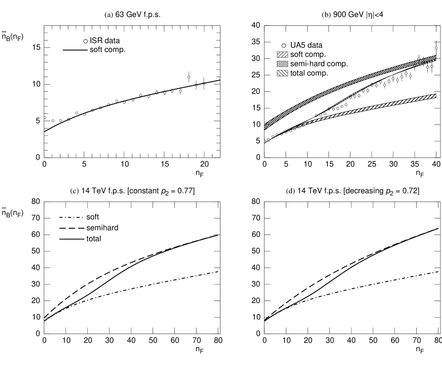
Figure 3: Results of our model for $\bar{n}_{B}(n_{F})$ vs. $n_{F}$ compared to experimental data [4, 9] in full phase-space at 63 GeV (a) and in the pseudo-rapidity interval $|\eta|<4$ at 900 GeV (b). Theoretical predictions at 14 TeV in f.p.s. for constant $p_{2}$ (c) and $p_{2}$ decreasing logarithmically with energy (d) are also shown.

Following the von Bahr-Ekspong theorem [15], in fact, the linear behaviour of $\bar{n}_{B}(n_{F})$ vs. $n_{F}$, the binomial distribution of particles in the forward and backward hemispheres and the occurrence of the NBMD are not independent statements. They are strongly linked: the validity of any two of them implies the validity of the third. It is clear that the linearity of the relation is violated in the soft and semi-hard components separately in our approach: in fact, it should be pointed out that in the first step of the production process clans, not particles, are binomially distributed in the two hemispheres with $p=1/2$, and that in the second step each clan generates particles, binomially distributed in the two hemispheres but with $p_{1}$ and $p_{2}$ different from 1/2. Accordingly, the final particles are not binomially distributed in the two hemispheres. Being the multiplicity distribution of the two classes of events a NBMD, the linearity of FB multiplicity correlations in each substructure cannot be exact. An example of a mild violation of linearity in the soft component is shown in Fig. 3(a) where $\bar{n}_{B}(n_{F})$ is plotted vs. $n_{F}$ at ISR energies (63 GeV). In addition, the extremely good fit of experimental data obtained by using a single NB(Pascal)MD for describing this component which in this case represents the total MD (at this energy the semi-hard component has been assumed to be negligible) is an indirect confirmation of the validity of our argument. Of course by going to higher c.m. energies in $pp$ collisions one expects that the linearity violation occur not only in the soft component but also in the semi-hard one. The linearity violation in each separate components is shown in Fig. 3(b) at 900 GeV c.m energy: parameters from the two fits proposed in [11] have been used; their values determine the borders of the bands shown in the figure; the $p_{2}$ parameter has been taken equal to 0.77.

It should be pointed out that since the total multiplicity distribution resulting from the weighted superposition of events of the two separate substructures (with and without mini-jets) is not of NB type, and in view of the lack of binomial structure in the final charged particles MD in the two hemispheres, the linear behaviour of $\bar{n}_{B}(n_{F})$ vs. $n_{F}$ can in principle be restored for the total MD in agreement with the von Bahr-Ekspong theorem.

In Fig. 3(c) and (d), predictions at 14 TeV by using the parameters of the QCD-inspired scenario (labelled 3B in our notation) are given for $p_{2}=0.77$ as in the GeV region and for $p_{2}$ logarithmically decreasing with c.m. energy in the TeV region ($p_{2}=0.72$ at 14 TeV). They confirm the general trend of $\bar{n}_{B}(n_{F})$ vs. $n_{F}$ seen at 900 GeV. The previously discussed scenarios 1B and 2B lead in this case to very small modification (not shown).

Some comments are needed in order to understand the theoretical predictions of the weighted superposition mechanism of the soft and semi-hard components for the general trend of $\bar{n}_{B}(n_{F})$ vs. $n_{F}$ and its linear behaviour found experimentally in $|\eta|<4$ at 900 GeV by UA5 Collaboration (Fig. 3(b)).

The theoretical predictions are based on a separation of the two components which comes from fits [11] to the total charged MD and not from an event-by-event classification. The idea of separating the total class of events into two components is correct in principle—as we have shown in our work—but is questionable here in its application. Different sets of NB parameters for the two components could lead to good fits of the total charged MD. Two sets we used are taken from [11] and their predictions collected in bands in Fig. 3(b). Results should be considered therefore only indicative of the general trend, which we consider quite satisfactory, especially for large $n_{F}$ values in the semi-hard component and small $n_{F}$ values in the soft one, as visible in the figure.

The second warning comes from intrinsic limitations of our approach. The choice to perform our study analytically led us to consider the $p_{1}$ and $p_{2}$ parameters approximately constant throughout the GeV region, an approximation which might turn out to be not correct and in any case to imply small modifications of our results.

In addition our predictions are based on the separation of the events into two classes. The onset of a third class of the same kind as that which could modify the $b$ bending effect described in Fig. 2—when properly inserted in our approach—could lead to different results.

All these considerations apply of course also to the FB multiplicity correlation strength energy dependence discussed in Fig. 2 and testify that our predictions, in view of the lack of detailed experimental data, should be considerd only indicative of the expected general trends.

5 Conclusions

General formulas for FB multiplicity correlation strength in the framework of the superposition mechanism of two weighted MD’s for different classes of events as functions of the average charged particle multiplicities and dispersions of each class of events are given. Assuming NB regularity behaviour for 2- and 3-jet samples of events in $e^{+}e^{-}$ annihilation at LEP energy, results obtained by OPAL collaborations are correctly reproduced within experimental errors in terms of the pure superposition effect, being FB multiplicity correlation strengths for the two separate classes of events negligible.

The same approach has been successfully extended to $pp$ collisions. Differently from $e^{+}e^{-}$ annihilation, the FB multiplicity correlation strengths in the two substructures (soft and semi-hard events) turn out to be quite important and to lead to interesting predictions in the TeV region in the three scenarios discussed by the Authors in a previous paper and based on extrapolations of $pp$ collisions properties in the GeV region.

In particular an interesting connection is found between the particle populations within clans, particle leakage from clans in one hemisphere to the opposite hemisphere and superposition effect between different substructure of the collision. This finding favours structures with larger particle populations per clans and the decrease of the average number of clans. The FB charged particle multiplicity correlation strength is predicted to bend in all scenarios in the TeV region.

The effects of the main assumptions of the present approach on the linear relation between the average number of particles emitted in one hemisphere as function of particle emitted in the opposite hemisphere have also been studied and their expected general trend at LHC explored.

References

- [1] K. Alpgård et al. (UA5 Collaboration), Phys. Lett. B123, 361 (1983).
- [2] G.J. Alner et al. (UA5 Collaboration), Physics Reports 154, 247 (1987).
- [3] J. Benecke and J.H. Kühn, Nucl. Phys. B140, 179 (1978).
- [4] S. Uhlig et al, Nucl. Phys. B132, 15 (1978).
- [5] V.V. Aivazyan et al. (NA22 Collaboration), Z. Phys. C42, 533 (1989).
- [6] R. Akers et al. (OPAL Collaboration), Phys. Lett. B320, 417 (1994).
- [7] P. Abreu et al. (DELPHI Collaboration), Z. Phys. C50, 185 (1991).
- [8] W. Braunschweig et al. (TASSO Collaboration), Z. Phys. C45, 193 (1989).
- [9] R.E. Ansorge et al. (UA5 Collaboration), Z. Phys. C37, 191 (1988).
- [10] A. Giovannini, S. Lupia and R. Ugoccioni, Phys. Lett. B374, 231 (1996).
- [11] C. Fuglesang, in Multiparticle Dynamics: Festschrift for Léon Van Hove, edited by A. Giovannini and W. Kittel (World Scientific, Singapore, 1990), p. 193.
- [12] A. Giovannini and R. Ugoccioni, Phys. Rev. D59, 094020 (1999).
- [13] J. Dias de Deus, J. Kwiecinski and M. Pimenta, Phys. Lett. B202, 397 (1988).
- [14] P. Carruthers and C.C. Shih, Phys. Lett. B165, 209 (1985).
- [15] G. Ekspong, in Multiparticle Dynamics: Festschrift for Léon Van Hove, edited by A. Giovannini and W. Kittel (World Scientific, Singapore, 1990), p. 467.