DFPD 02/TH/10

GAUGE SYMMETRY BREAKING ON ORBIFOLDS

We discuss a new method for gauge symmetry breaking in theories with one extra dimension compactified on the orbifold $S^{1}/Z_{2}$. If we assume that fields and their derivatives can jump at the orbifold fixed points, we can implement a generalized Scherk-Schwarz mechanism that breaks the gauge symmetry. We show that our model with discontinuous fields is equivalent to another with continuous but non periodic fields; in our scheme localized lagrangian terms for bulk fields appear.

Symmetries (and their breaking) play a fundamental role in theoretical high energy physics. In theories with extra dimensions new methods for symmetry breaking appear, such as the Scherk-Schwarz mechanism $\!{}^{{\bf?}}$, the Hosotani mechanism $\!{}^{{\bf?}}$ and the orbifold projection $\!{}^{{\bf?}}$.

In this paper we will focus on theories with one extra dimension compactified on the orbifold $S^{1}/Z_{2}$ where the radius of the circle $R$ is of order of $1/M_{GUT}$ $\!{}^{{\bf?}}$, with $M_{GUT}\approx 10^{16}Gev$, and the orbifold $Z_{2}$ is constructed by identifying points $(x,y)$ with points $(x,-y)$, where $x$ and $y$ are respectively the coordinates of the four and the fifth dimensions. The orbifold projection introduces two fixed points, at $y=0$ and $y=\pi R$. While on the circle the only boundary condition we can assign to fields is the one corresponding to the translation of $2\pi R$ (twist condition), on the orbifold we have to fix the parity and the behavior of fields at the fixed points, that means new possibilities are allowed $\!{}^{{\bf?}}$.

If we consider a set of $n$ 5-dimensional bosonic fields $\phi(x,y)$ $\!{}^{{\bf?}}$, the self-adjointness of the kinetic operator requires that we assign conditions also on the $y$-derivative of $\phi(x,y)$. We look for boundary conditions in the following class:

$$\left(\begin{array}[]{c}\phi\\ \partial_{y}\phi\end{array}\right)(\gamma^{+})=V_{\gamma}~{}\left(\begin{array}[]{c}\phi\\ \partial_{y}\phi\end{array}\right)(\gamma^{-})~{}~{},\\$$ (1)

where $\gamma=(0,\pi,\beta)$, $\gamma^{\pm}=(0^{\pm},\pi R^{\pm},y^{\pm})$, and $V_{\gamma}$ are constant $2n$ by $2n$ matrices. We have defined $0^{\pm}\equiv\pm\xi$, $\pi R^{\pm}\equiv\pi R\pm\xi$, with $\xi$ small positive parameter, $y^{-}\equiv y_{0}$ and $y^{+}\equiv y_{0}+2\pi R$, with $y_{0}$ for convenience chosen between $-\pi R+\xi$ and $-\xi$.

We now constrain the matrices $V_{\gamma}$. We require, first, that the boundary conditions preserve the self-adjointness of the kinetic operator $-\partial_{y}^{2}$ and, second, that physical quantities remain periodic and continuous even if fields are not. If the theory is invariant under the global transformations of a group G, these requirements imply the following form for the $V_{\gamma}$ matrices:

$$V_{\gamma}=\left(\begin{array}[]{cc}U_{\gamma}&0\\ 0&U_{\gamma}\end{array}\right)~{},$$ (2)

where $U_{\gamma}$ is an orthogonal $n$-dimensional representation of G. Finally we should take into account consistency conditions among the twist, the jumps and the action of orbifold on the fields, defined by the following equation:

$$\phi(-y)=Z\phi(y)~{}~{}.$$ (3)

We have:

$$U_{\gamma}~{}Z~{}U_{\gamma} = Z\qquad\qquad\gamma\in(0,\pi,\beta)$$

$$\left[U_{0},U_{\beta}\right] = 0$$ (4)

$$\left[U_{\pi},U_{\beta}\right] = 0~{}~{}.$$

If $\left[Z,U_{\gamma}\right]=0$ and $\left[U_{0},U_{\pi}\right]=0$ there is a basis in which $U_{\gamma}$ are diagonal with elements $\pm 1$; in this case twist and jumps are defined by discrete parameters. However if $\left[Z,U_{\gamma}\right]\neq 0$ or $\left[U_{0},U_{\pi}\right]\neq 0$ continuous parameter can appear in $U_{\gamma}$ and then in eigenfunctions and eigenvalues.

To show how we can exploit these boundary conditions to break a symmetry, we focus on the simple case of one real scalar field. We start by writing the equation of motion for $\phi$

$$-\partial^{2}_{y}\phi=m^{2}\phi~{}~{},$$ (5)

in each region $y_{q}<y<y_{q+1}$, where $y_{q}\equiv q\pi R$ and $q\in Z$. We have defined the mass $m$ through the 4-dimensional equation $\partial^{2}\phi=m^{2}\phi$. The solutions of these equations can be glued by exploiting the boundary conditions $V_{0}$ and $V_{\pi}$, imposed at $y=y_{2q}$ and $y=y_{2q+1}$, respectively. Finally, the spectrum and the eigenfunctions are obtained by requiring that the solutions have the twist described by $V_{\beta}$. In this theory the group of global symmetry is a $Z_{2}$, so that $V_{\gamma}$ can be $\pm 1$.

We focus on one example in which we compare the usual Scherk-Schwarz mechanism with our generalized one. We consider even fields and the following two sets of boundary conditions:

$$(U_{0},U_{\pi},U_{\beta})~{}=~{}\left\{\begin{array}[]{cc}(+1,+1,-1)&~{}~{}~{}~{}~{}(\textrm{A})\\ (+1,-1,+1)&~{}~{}~{}~{}~{}(\textrm{B})\end{array}\right..$$ (6)

In the first case fields are continuous but antiperiodic; the solution to the eq. of motion with these boundary conditions is:

$$\phi^{A}(x,y)=\alpha(x)~{}cos(my)\qquad\qquad\qquad\quad mR=n+\frac{1}{2}~{}~{}.$$ (7)

In the case (B) fields are periodic but with a jump in $y=\pi R$; the solution is:

$$\phi^{B}(x,y)=\beta(x)~{}\epsilon\left(\frac{y}{2}+\frac{\pi R}{2}\right)~{}cos(my)~{}~{}~{}~{}~{}~{}mR=n+\frac{1}{2}~{}~{},$$ (8)

where $\epsilon(y)$ is the sign function on $S^{1}$.

   

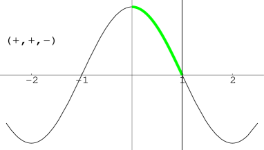
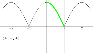
Figure 1: Eigenfunctions of $-\partial_{y}^{2}$ versus $y/(\pi R)$, in cases (A) and (B).

The spectrum is the same in both cases and it is the Kaluza-Klein tower $n/R$ shifted by $1/2R$. This is just what we expected in case (A), because this is precisely the Scherk-Schwarz mechanism: when fields are not periodic, their spectra are shifted from the Kaluza-Klein levels by an amount depending on the twist and zero modes are removed. If $\phi$ is a gauge field of a multiplet containing also untwisted fields, this is a mechanism for symmetry breaking. As we have already observed the (B)-spectrum is identical to the (A)-spectrum; this means that we can break a symmetry not only through a twist, but also with discontinuities. While the spectra are identical, eigenfunctions (see fig. 1) are different, but they are related by a simple field redefinition:

$$\phi^{B}(x,y)~{}=~{}\epsilon\left(\frac{y}{2}+\frac{\pi R}{2}\right)~{}\phi^{A}(x,y)~{}~{}.$$ (9)

The equation (9) is a map between a system in which fields are continuous and twisted (A) and another in which fields are discontinuous and periodic (B). In order to show the two schemes are completely equivalent, we should perform the field redefinition at the level of the action and, using the eq. of motion, recover the eigenfunction and the spectrum. After the field redefinition, the lagrangian for the massless real scalar field becomes:

$$\mathcal{L}(\phi,\partial\phi)=\frac{1}{2}\epsilon^{2}\partial_{M}\phi~{}\partial^{M}\phi-2~{}\epsilon~{}\delta_{\pi R}~{}\phi~{}\partial_{y}\phi+2~{}\delta_{\pi R}^{2}~{}\phi^{2}~{}~{},$$ (10)

where $\epsilon=\epsilon(y/2+\pi R/2)$ and $\delta_{y_{0}}=\delta(y-y_{0})$. The new lagrangian contains two quadratic terms localized at $y=\pi R$. Now we want to derive the equation of motion for $\phi$, but the naive application of the variational principle would lead to inconsistent results: indeed this works with continuous functions, but $\phi$ are discontinuous. In order to derive the correct equation of motion we regularize $\epsilon$ with a smooth function $\epsilon_{\lambda}$ wich reproduces $\epsilon$ in the limit $\lambda\rightarrow 0$. If we now rewrite the lagrangian (10) in term of $\epsilon_{\lambda}$ and continuous fields, derive the equation of motion and then perform the limit $\lambda\rightarrow 0$, we obtain:

$$\epsilon\partial_{y}^{2}\phi-4\delta_{\pi R}\partial_{y}\phi-2\delta_{\pi R}^{\prime}\phi+\epsilon m^{2}\phi=0$$ (11)

Away from the point $y=\pi R$ this equation reduces to the one for continuous fields, while integrating it around the fixed point the singular terms give us the expected jumps. With this procedure we have shown that the continuous framework is really equivalent to the discontinuous one.

If we consider two or more real scalar fields such as a complex scalar field or a gauge field, continuous parameters are allowed in the boundary conditions and then they are also present in the eigenfunctions and in the spectra. It is interesting to note that, being the shift from the Kaluza-Klein spectrum continuous, we can go continuously from a phase in which the symmetry is broken to another in which it is unbroken.

Table 1: Boundary conditions, eigenfunctions and spectra for fields in the Kawamura model in the traditional scheme ($2^{nd}$, $3^{rd}$ and $6^{th}$ columns) and in our framework ($4^{th}$, $5^{th}$ and $6^{th}$ columns).

Fields	$(Z_{2},U_{\beta})$	${\textrm{Kawamura}\atop\textrm{eigenfunctions}}$	$(Z_{2},U_{\pi})$	${\textrm{Our}\atop\textrm{eigenfunctions}}$	${\textrm{Spectrum}\atop m}$
$A^{a}_{\mu},\lambda_{L}^{2a},H^{D}_{u},H^{D}_{d}$	$(+,+)$	$cos(my)$	$(+,+)$	$cos(my)$	$\frac{2n}{R}$
$A^{\hat{a}}_{\mu},\lambda_{L}^{2\hat{a}},H^{T}_{u},H^{T}_{d}$	$(+,-)$	$cos(my)$	$(+,-)$	$\epsilon(\frac{y}{2}+\frac{\pi R}{2})cos(my)$	$\frac{2n+1}{R}$
$A^{\hat{a}}_{5},\Sigma^{\hat{a}},\lambda_{L}^{1\hat{a}},\hat{H}^{T}_{u},\hat{H}^{T}_{d}$	$(-,-)$	$sin(my)$	$(-,-)$	$\epsilon(\frac{y}{2}+\frac{\pi R}{2})sin(my)$	$\frac{2n+1}{R}$
$A^{a}_{5},\Sigma^{a},\lambda_{L}^{1a},\hat{H}^{D}_{u},\hat{H}^{D}_{d}$	$(-,+)$	$sin(my)$	$(-,+)$	$sin(my)$	$\frac{2n+2}{R}$

We use now our mechanism to break the symmetries of a grand unified theory defined on the orbifold $S^{1}/Z_{2}$ $\!{}^{{\bf?},{\bf?}}$. The model we consider is the one constructed by Kawamura $\!{}^{{\bf?}}$ in which the lagrangian is invariant under the transformations of an $SU(5)$ gauge group and $N=2$ (from the 4-dimensional point of view) supersymmetry. The fields content is the following: there is a vector multiplet $V=(A^{\alpha}_{M},\lambda^{1\alpha}_{L},\lambda^{2\alpha}_{L},\Sigma^{\alpha})$, with $\alpha=1,...,24$ and $M=\mu,5$ which forms an adjoint representation of $SU(5)$, and two hypermultiplets $H^{1}$ and $H^{2}$, equivalent to four chiral multiplets $H_{5}$, $\hat{H_{\overline{5}}}$, $\hat{H_{5}}$ and $H_{\overline{5}}$ which form two fundamental representations of $SU(5)$. These are multiplets of $N=1$ supersymmetry in 5 dimensions, that is equivalent to $N=2$ supersymmetry in 4 dimensions. The gauge vector bosons are the fields $A^{\alpha}_{M}$: $A^{a}_{M}$ with $a=1,...,12$ are the vector bosons of the standard model, while $A^{\hat{a}}_{M}$ with $\hat{a}=13,...,24$ are those of the coset $SU(5)~{}/~{}SU(3)\times SU(2)\times U(1)$.

In table 1 (second column) parity and twist assignments for all fields are shown, together with the resulting eigenfunctions and spectra (third and last columns). We see that these parity assigments alone break supersymmetry from $N=2$ to $N=1$, because zero modes survive only for even fields (without twist the spectrum would be $n/R$ in all cases). When we assign a non trivial twist to fields, their spectra are shifted from the usual Kaluza-Klein tower. With the assignments of table 1 the only fields that mantain a zero mode are the vector bosons of the standard model, $A_{\mu}^{a}$, their supersymmetric partners, $\lambda^{2a}_{L}$, and two Higgs doublets $H^{D}_{u}$ and $H^{D}_{d}$: precisely the fields of the Minimal Supersymmetric Standard Model, that is $SU(3)_{c}\times SU(2)_{L}\times U(1)_{Y}$ with $N=1$ supersymmetry. We observe that with these boundary conditions also the doublet-triplet splitting problem is naturally solved, because the lightest triplets modes are of order of $1/R$, while doublets have zero modes.

Up to now only gauge and Higgs fields and their supersymmetric partners have been considered. If we introduce fermions and we assign the appropriate boundary conditions $\!{}^{{\bf?}}$ we can see that fast proton decay is avoided. Then this model can be a realistic Grand Unified Theory and we adopt it to show in details how our mechanism for gauge symmetry breaking works.

In our framework parity assignments are identical to the original ones, but, instead of a twist, we require that some fields jump in $y=\pi R$. Among gauge fields only the vector bosons of the coset $SU(5)~{}/~{}SU(3)\times SU(2)\times U(1)$ jump. In the last three columns of table 1 boundary conditions, eigenfunctions and eigenvalues are shown. We can observe that the spectra are the same of the Kawamura model for all fields, while eigenfunctions are identical for continuous fields but different for jumping fields. If we look at their explicit forms we observe we are just in the case studied before with one real scalar field. Performing the field redefinition of eq. (9), where ‘A’ fields are Kawamura’s eigenfunctions and ‘B’ fields are ours, we see the two frameworks are completely equivalent.

What about the lagrangians? Following the lines of what we did in the scalar case, we can perform the field redefinition at the level of the action in order to find the localized terms related to jumps in this theory. For simplicity we consider only the Yang-Mills term of the lagrangian, neglecting both the supersymmetric part and the Higgs terms:

$$\mathcal{L}=-\frac{1}{4}F^{\alpha}_{MN}F^{\alpha MN}~{}~{}.$$ (12)

Applying the redefinition (9) this becomes:

$$-\frac{1}{4}\tilde{F}^{a}_{MN}\tilde{F}^{aMN}+\frac{1}{2}\epsilon^{2}f^{a\hat{b}\hat{c}}A^{\hat{b}}_{M}A^{\hat{c}}_{N}\tilde{F}^{aMN}+$$

$$-\frac{1}{4}\epsilon^{4}f^{a\hat{b}\hat{c}}f^{a\hat{d}\hat{e}}A^{\hat{b}}_{M}A^{\hat{c}}_{N}A^{\hat{d}M}A^{\hat{e}N}-\frac{1}{4}\epsilon^{2}F^{\hat{a}}_{MN}F^{\hat{a}MN}+$$ (13)

$$-2~{}\delta_{\pi R}^{2}~{}(A^{\hat{a}}_{N}A^{\hat{a}N}-A^{\hat{a}}_{5}A^{\hat{a}5})+2~{}\epsilon~{}\delta_{\pi R}~{}F^{\hat{a}}_{5N}A^{\hat{a}N}~{}~{},$$

where $\tilde{F}^{a}_{MN}=\partial_{M}A^{a}_{N}-\partial_{N}A^{a}_{M}-f^{abc}A^{b}_{M}A^{c}_{N}$. We observe that the last two terms are localized at the fixed point $y=\pi R$. While the first is simply a bilinear term, as the ones found in the case of one scalar field, the last contains also a trilinear part:

$$2~{}\epsilon~{}\delta_{\pi R}~{}F^{\hat{a}}_{5N}A^{\hat{a}N}=2~{}\epsilon~{}\delta_{\pi R}~{}[(\partial_{5}A^{\hat{a}}_{N}-\partial_{N}A^{\hat{a}}_{5})A^{\hat{a}N}+f^{\hat{a}b\hat{c}}A^{\hat{a}N}A^{b}_{N}A^{\hat{c}}_{5}].$$ (14)

This last term is proportional to the fields $A^{\hat{c}}_{5}$ that are just the ‘would-be’ Goldstone bosons that give mass to the Kaluza-Klein modes of the gauge vector bosons of the coset $SU(5)/SU(3)\times SU(2)\times U(1)$.

In the previuos pages we always started from the continuous theory and then we derived the localized lagrangian terms, exploiting a relation found between smooth and jumping eigenfunctions. But our reasoning can be reversed: we can try to reabsorb localized terms for bulk fields through a field redefinition. This kind of terms are very common in theories with extra dimensions $\!{}^{{\bf?}}$, and showing they are only the effect of some discontinuities of the fields would improve our control of the theory. In our work we have shown that in some cases this is possible.

In summary in this paper we have shown how the Scherk-Schwarz mechanism works with discontinuous fields, in particular with bosonic fields. We have analyzed in detail the constraints on the generalized boundary conditions and we have shown the connection between the smooth framework and the discontinuous one in the case of one real scalar field. Then we have applied our mechanism to a Grand Unified Theory based on the $SU(5)$ gauge group that breaks down to $SU(3)\times SU(2)\times U(1)$ and we have shown how localized terms for bulk fields appear in the lagrangian. We have observed that these terms are strictly related to discontinuities of fields at the fixed points and that in some cases they can be reabsorbed through a field redefinition.

References

References

- [1] J. Scherk and J.H. Schwarz, Nucl. Phys. B 153, 61 (1979); Phys. Lett. B 82, 60 (1979).
- [2] Y. Hosotani, Phys. Lett. B 126, 309 (1983); Ann. Phys. 190, 233 (1989).
- [3] L.J. Dixon, J.A. Harvey, C. Vafa and E. Witten, Nucl. Phys. B 261, 678 (1985); Nucl. Phys. B 274, 285 (1986).
- [4] P. Fayet, Phys. Lett. B 146, 41 (1984).
- [5] J.A. Bagger, F. Feruglio and F. Zwirner, Phys. Rev. Lett. 88, 101601 (2002).
- [6] C. Biggio and F. Feruglio, in preparation.
-
[7]
A lot of models have been constructed on orbifolds;
see for example:
R. Barbieri, L.J. Hall and Y. Nomura, Phys. Rev. D 63, 105007 (2001); hep-ph/0106190; Nucl. Phys. B 624, 63 (2002); hep-ph/0110102;
L.J. Hall, H. Murayama and Y. Nomura, hep-th/0107245;
L.J. Hall and Y. Nomura, Phys. Rev. D 64, 055003 (2001); hep-ph/0111068; Phys. Lett. B 532, 111 (2002); hep-ph/0205067;
A. Hebecker and J. March-Russel, Nucl. Phys. B 613, 3 (2001); Nucl. Phys. B 625, 128 (2002); hep-ph/0204037;
E.A. Mirabelli and M.E. Peskin, Phys. Rev. D 58, 065002 (1998);
I. Antoniadis, Phys. Lett. B 246, 377 (1990);
I. Antoniadis, C. Munoz and M. Quiros, Nucl. Phys. B 397, 515 (1993);
A. Pomarol and M. Quiros, Phys. Lett. B 438, 255 (1998);
I. Antoniadis, S. Dimopoulos, A. Pomarol and M. Quiros, Nucl. Phys. B 544, 503 (1999);
A. Delgado, A. Pomarol and M. Quiros, Phys. Rev. D 60, 095008 (1999); JHEP 0001, 030 (2000);
A. Delgado and M. Quiros, Nucl. Phys. B 559, 235 (1999); Phys. Lett. B 484, 355 (2000); Nucl. Phys. B 607, 99 (2001);
A. Delgado, G. von Gersdorff, P. John and M. Quiros, Phys. Lett. B 517, 445 (2001);
A. Delgado, G. von Gersdorff and M. Quiros, Nucl. Phys. B 613, 49 (2001);
V. Di Clemente, S.F. King and D.A.J. Rayner, Nucl. Phys. B 617, 71 (2001); hep-ph/0205010. - [8] Y. Kawamura, Prog. Theor. Phys. 105, 999 (2001).
- [9] G. Altarelli and F. Feruglio, Phys. Lett. B 511, 257 (2001).
-
[10]
H. Georgi, A.K. Grant and G. Hailu, Phys. Rev. D 63, 064027 (2001); Phys. Lett. B 506, 207 (2001);
N. Arkani-Hamed, L.J. Hall, Y. Nomura, D.R. Smith and N. Weiner, Nucl. Phys. B 605, 81 (2001);
J.A. Bagger, F. Feruglio and F. Zwirner, JHEP 0202, 010 (2002);
C.A. Scrucca, M. Serone, L. Silvestrini and F. Zwirner, Phys. Lett. B 525, 169 (2002);
C.A. Scrucca, M. Serone and M. Trapletti, hep-th/0203190;
R. Barbieri, R. Contino, P. Creminelli, R. Rattazzi and C.A. Scrucca, hep-th/0203039;
L. Pilo and A. Riotto, hep-th/0202144;
S. Groot Nibbelink, H.P. Nilles and M. Olechowski, hep-th/0203055; hep-th/0205012.