In this article I summarize some aspects of the current status of the field of high energy physics and discuss how the next generation of high energy colliders will aid in furthering our basic understanding of elementary particles and interactions among them, by shedding light on the mechanism for the spontaneous breakdown of the Electroweak Symmetry.

1 Introduction:

Particle physics is at an extremely interesting juncture at present. The theoretical developments of the last 50 years have now seen establishment of quantum gauge field theories as the paradigm for the description of fundamental particles and interactions among them. The Standard Model of particle physics (SM) which provides a description of particle interactions in terms of a Quantum Gauge Field Theory with $SU(3)_{C}$ X $SU(2)_{L}$ X $U(1)$ gauge invariance, has been shown to describe all the experimental observations in the area of electromagnetic, weak and strong interactions of quarks and leptons. The predictions of the Electroweak (EW) theory have been tested to an unprecedented accuracy. These predictions involve effects of loop corrections, which can be calculated in a consistent way only for a renormalizable theory and the theories are guaranteed to be renormalizable, if they are gauge invariant. Naively, the gauge invariance is guarunteed only if the corresponding gauge boson is massless. The massless $\gamma$ is an example. Developement of a unified theory of electromagnetic and weak interactions in terms of a gauge invariant quantum field theory (QFT) took place in the 70s and 80s. The theoretical cornerstone of these developments was the proof that these theories are renormalizable even in the presence of nonzero masses of the corresponding gauge bosons W and Z; the so called spontaneous breakdown of the gauge symmetry. The first experimental proof in favour of the EW theory came in the form of the discovery of neutral current interactions in 1973, whereas the first direct experimental observationxs of the massive gauge bosons came in 1983 at the S$\bar{p}$pS collider. The measurement of the masses of the W and Z bosons in these experiments, their agreement with the predictions of the Glashow, Salam and Weinberg (GSW) model in terms of a single parameter $sin^{2}\theta_{W}$ determinded experimentally from a variety of data and the verification of the relation $\rho$ = $\frac{m^{2}_{W}}{m^{2}_{Z}cos^{2}\theta_{W}}=1$ were the various milestones in the establishment of the GSW model as the correct theory of EW interactions as an SU(2) X U(1) gauge theory at the tree level. However, the correctness of this theory at the loop level was proved conclusively only by the spectacular agreement of the value of $m_{t}$ obtained from direct observations of the top quark at the $\bar{p}$p collider Tevatron ($m_{t}=174.3\pm 5.1$ GeV) with the one obtained indirectly from the precision measurements of the properties of the Z boson at the $e^{+}e^{-}$ LEP and SLC colliders ($m_{t}=180.5\pm 10.0$ GeV). Direct observations of the effects of the trilinear WWZ coupling, reflecting the nonabelian nature of the $SU(2)_{L}$ X U(1) gauge theory through the direct measurement of the energy dependence of $\sigma(e^{+}e^{-}\to W^{+}W^{-})$ at the second stage of $e^{+}e^{-}$ collider LEP (LEP2) also was an important milestone. As a result of a variety of high precision measurements in the EW processes, the predictions of the SM as a QFT with $SU(3)_{C}$ X $SU(2)_{L}$ X $U(1)$ gauge invariance, have now been tested to an accuracy of 1 part in $10^{6}$. Fig. 1 from [1] shows the

Figure 1: Precision measurements at the $e^{+}e^{-}$ colliders LEP/SLC and ‘pull’

precision measurements of a large number of observables at LEP/SLC alongwith their best fit values to the SM in terms of $m_{Z}$, $\alpha_{em}$ and the nuclear $\beta$ decay, Fermi coupling constant $G_{F}$. The third column shows the ‘pull’, i.e., the difference between the SM fit value and the measurements in terms of standard deviation error of the measurement. It is interesting that due to the very high precision of these measurements the $\chi^{2}/dof$ is $22.9/15$ in spite of the very good quality of fits provided by the SM. The possible precision now even allows extracting indirect information on the Higgs mass, just the same way the earlier LEP measurements at the Z-pole, gave the top mass indirectly. In spite of this impressive success of the SM, in describing every piece of measurement in high energy experiments so far (with the possible exception of the $(g-2)_{\mu}$ measurement [2]), the complete truth of the SM will not be established satisfactorily until one finds ‘direct’ evidence for the Higgs scalar. In addition to this we should also remember that although the beautiful experiments at HERA and Tevatron, have confirmed the predictions of perturbative QCD in the domain of large $Q^{2}$, there has been no ‘direct’ observation of the ‘unconfined’ quarks and gluons. In the next section I first discuss why the idea of the Higgs boson forms the cornerstone of the SM model. Further I point out the arguments which show that either a Higgs scalar should exist in the mass range indicated by the current precision measurements [1], or there should exist (with a very high probability) some alternative physics at $\sim$ TeV scale which would provide us with a clue to an understanding of the phenomenon of spontaneous breakdown of the EW symmetry. In the next section I will discuss what light will the experiments at the Tevatron in near future be able to shed on the problem. I will not, however, be able to survey what information the currently running experiment at Relativistic Heavy Ion Collider (RHIC) will provide about the theory of strong interactions, QCD, in a domain not accessible to perturbative quantum computation. I will end by discussing the role that the future colliders will play in unravelling this last knot in our understanding of fundamental particles and interactions among them. These future colliders consist of the pp collider, Large Hadron Collider (LHC) which is supposed to go in action in 2007 and will have a total c.m. energy of 18 TeV and the higher energy $e^{+}e^{-}$ linear colliders with a c.m. energy between $350$ GeV and $1000$ GeV, which are now in the planning stages.

2 The spontaneous breakdown of EW symmetry and new physics at the TeV scale

Requiring that cross-sections involving weakly interacting particles satisfy unitarity, viz., they rise slower than $\log^{2}(s)$ at high energies, played a very important role in the theoretical development of the EW theories. Initially the existence of intermediate vector bosons itself was postulated to avoid ‘bad’ high energy rise of the neutrino cross-section. Note that possible violations of unitarity for the cross-section $\bar{\nu_{\mu}}$ $\mu\to\bar{\nu_{e}}$ e for E $<$ $G_{F}^{-1/2}$ $\sim$ 300 GeV is cured in reality by a $W^{-}$ boson of a much lower mass $\sim$ 80 GeV. Further, the need for a nonabelian coupling as well as the existence of a scalar with couplings to fermions/gauge bosons proportional to their masses can be inferred  [3] from simply demanding good high energy behaviour of the cross-section $e^{+}e^{-}\rightarrow W^{+}W^{-}$. Left panel in Fig. 2 shows the data on $W^{+}W^{-}$ production cross-section from LEP2. The data show the flattening of $\sigma$ ($e^{+}e^{-}\to W^{+}W^{-}$) at high energies clearly demonstrating the existence of the ZWW vertex as well as that of the interference between the t-channel $\nu_{e}$ exchange and s-channel $\gamma^{*}/Z^{*}$ exchange diagrams. These diagrams are indicated in the figure in the panel on the r.h.s. which shows the behaviour of the same cross-section at much higher energies along with the contributions of the individual diagrams [4]. This figure essentially shows how the measurements of this cross-section at higher energies will test this feature of the SM even more accurately.

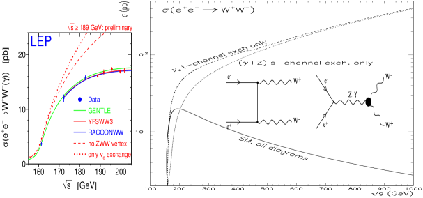
Figure 2: The small insert shows the latest data of the $W^{+}W^{-}$ cross section at LEP2[1]. The main figure shows the behaviour of the same cross section at much higher energies and the contribution of each channel.

As mentioned in the introduction, one way to formulate a consistent, renormalizable gauge field theory, is via the mechanism of spontaneous symmetry breakdown of the $SU(2)_{L}XU(1)$ gauge symmetry, whose existence has been proved incontrovertially by the wealth of precision measurements. Though the mechanism predicts the Higgs scalar and gives the couplings of this scalar in terms of gauge couplings, its mass is not predicted.

The above discussion mentions the connection between unitarity and existence of a Higgs scalar. Demanding $s$ wave unitarity of the process $W^{+}W^{-}\to W^{+}W^{-}$ can actually give an upper limit on the mass of the Higgs. Without the Higgs exchange diagram one can show that the amplitude for the process $W^{+}_{L}W^{-}_{L}\to W^{+}_{L}W^{-}_{L}$ will grow with energy and violate unitarity for $\sqrt{s_{WW}}\geq$ 1.2 TeV, implying thereby that some physics beyond the gauge bosons alone, is required somewhere below that scale to tame this bad high energy behaviour. The addition of Higgs exchange diagrams tames the high energy behaviour somewhat. Demanding perturbative unitarity for the J=0 partial wave amplitudes for $W^{+}_{L}W^{-}_{L}\to W^{+}_{L}W^{-}_{L}$ gives a limit on the Higgs mass $m_{h}\leq\sim$ 700 GeV  [5]. These arguments tell us that just a demand of unitarity implies that some new physics other than the gauge bosons must exist at a TeV scale. Specializing to the case of the SM where spontaneous symmetry breakdown happens via Higgs mechanism, the scale of the new physics beyond just gauge bosons and fermions is lowered to 700 GeV.

Within the framework of the SM, Higgs mass $m_{h}$ is also restricted by considerations of vacuum stability as well as that of triviality of a pure $\Phi^{4}$ field theory. The demand that the Landau pole in the self coupling $\lambda$, lies above a scale $\Lambda$ puts a limit on the value of $\lambda$ at the EW scale which in turn limits the Higgs mass $m_{h}$. This requirement essentially means that the Standard Model is a consistent theory upto a scale $\Lambda$ and no other physics need exist upto that scale. The left panel in Fig.3 taken from [6] shows the region in $m_{h}$ - $\Lambda$ plane that is allowed by these considerations, the lower limit coming from demand of vacuum stability. Note that for $\Lambda$ $\sim$ 1 TeV, the limit on $m_{H}$ is $\sim$ 800 GeV, completely consistent with the unitarity argument presented above.

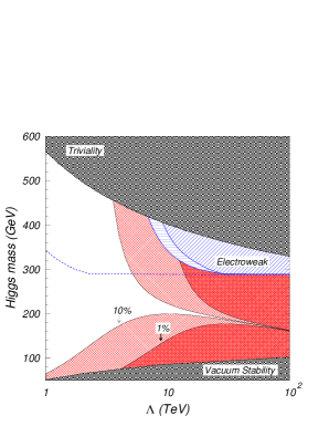
Figure 3: Limits on the Higgs mass in the SM and beyond[6, 7].

As mentioned in the introduction, the knowledge on $m_{t}$ from direct observation and measurements at the Tevatron, now allows one to restrict $m_{h}$ by considering the dependence of the EW loop corrections to the various EW observables

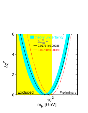
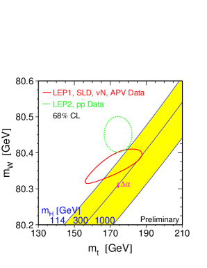
Figure 4: (left panel) $\Delta\chi^{2}$ as a function of $m_{h}$ for a fit to the SM of the precision measurements at LEP and (right panel) consistency between the direct and indirect measurements of $m_{t},m_{W}$ [1],

listed in Fig.1 on $m_{h}$. The left panel of Fig. 4 [1] shows the value of $\Delta\chi^{2}$ for the SM fits as a function of $m_{h}$. Boundary of the shaded area indicates the lower limit on $m_{h}$ implied by direct measurements at LEP2, $m_{h}$ $<$ 113 GeV. Consistency of the upper limit of 196 GeV (222 GeV) for two different choices of $\Delta\alpha_{had}$ listed on the figure, with the range of 160 $\pm$ 20 geV predicted by the SM (cf. Fig. 3 left panel) for $\Lambda$ = $M_{pl}$ is very tantalizing. The two ovals in the right panel of the Fig. 4 show the indirectly and directly measured values of $m_{t},m_{W}$ along with the lines of the SM predictions for different Higgs masses. First this shows clearly that a light Higgs is preferred strongly in the SM. Further we can see that an improvement in the precision of the $m_{W}$ and $m_{t}$ measurement will certainly help give further indirect information on the Higgs sector and hence will allow probes of the physics beyond the SM, if any should be indicated by the data in future experiments. Note that the $m_{H}$ in the labels on the axes in Figs. 3 and 4 is the same as $m_{h}$ used in the text.

Recently more general theoretical analyses of correlations of the scale of new physics and the mass of the Higgs have started[7, 8]. In these the assumption is that the SM is only an effective theory and additional higher dimensional operators can be added. Based on very general assumptions about the coefficients of these higher dimensional operators, an analysis of the precision data from LEP-I with their contribution to the observables, alongwith a requirement that the radiative corrections to the $m_{h}$ do not destabilize it more than a few percent, allows different regions in $m_{h}-\Lambda$ plane. This is shown in the right panel in Fig. 3. The lesson to learn from this figure taken from Ref. [7] is that a light higgs with $m_{h}<130$ GeV will imply existence of new physics at the scale $\Lambda<2-3$ TeV, whereas $195<m_{h}<215$ GeV would imply $\Lambda_{Np}<10$ TeV.

We thus see that the theoretical consistency of the SM as a field theory with a light Higgs implies scale of new physics between 1 to 10 TeV. Conversely, the Higgs mass itself is severely constrained if SM is the right description of physics at the EW scale (at least as an effective theory) which is the case as shown by the experiments. If the physics that tames the bad high energy behaviour of the EW amplitudes is not given by the Higgs scalar, it would imply that there exist some nonperturbative physics giving rise to resonances corresponding to a strongly interacting $W^{+}W^{-}$ sector. This should happen at around a TeV scale.

Such a sector is implied in a formulation of a gauge invariant theory of EW interactions, without the elementary Higgs. However, in this case, one has to take recourse to the nonlinear realization of the symmetry using the Goldstone Bosons, but of course one with custodial symmetry which will maintain $\frac{M^{2}_{W}}{M^{2}_{Z}cos^{2}~{}\theta_{W}}=1$. One uses, (for notations and a mini review see [9])

$$\Sigma=exp(\frac{i\omega^{i}\tau^{i}}{v})\;\;\;{{\cal D}}_{\mu}\Sigma=\partial_{\mu}\Sigma+\frac{i}{2}\left(g{\mbox{\boldmath$W$}}_{\mu}\Sigma-g^{\prime}B_{\mu}\Sigma\tau_{3}\right)$$ (1)

The $W,Z$ masses are simply

$${\cal L}_{M}=\frac{v^{2}}{4}{\rm Tr}({\cal d}^{\mu}\Sigma^{\dagger}{\cal d}_{\mu}\Sigma)$$ (2)

which is the lowest order operator one can write.

The consistency of such a model with the LEP data which seems to require a light higgs is possible since the above mentioned fits are valid only within the SM. The fits to the precision measurements in this case are analysed in terms of the oblique parameters S, T, U [10]. It is necessary to consider additional new, higher dimensional operator which would give negative S [4, 9]

$${{\cal L}}_{10} = gg^{\prime}\frac{L_{10}}{16\pi^{2}}{\rm Tr}({\mbox{\boldmath$B$}}^{\mu\nu}\Sigma^{\dagger}{\mbox{\boldmath$W$}}^{\mu\nu}\Sigma)\longrightarrow L_{10}=-\pi S_{\rm New}$$ (3)

which breaks down the custodial symmetry somewhat. The earlier discussion of the higher dimensional operators involving both gauge and fermionic fields  [8] is a case where these ideas are taken a bit further. Howver, the fermionic operators were found to be strongly constrained there. The additional bosonic operators that one can write contribute to the trilinear and quartic couplings of the gauge bosons though not to the $S,T$ and $U$. For instance, ${{\cal L}}_{9L}=-ig\frac{L_{9L}}{16\pi^{2}}{\rm Tr}({\mbox{\boldmath$W$}}^{\mu\nu}{{\cal D}}_{\mu}\Sigma{{\cal D}}_{\nu}\Sigma^{\dagger})$ and ${{\cal L}}_{1}=\frac{L_{1}}{16\pi^{2}}\left({\rm Tr}(D^{\mu}\Sigma^{\dagger}D_{\mu}\Sigma)\right)^{2}$ to cite only two (for more see [9]). Now these operators need to be probed at higher energies. In order that one learns more than what we have with the LEP data, these operators should be constrained better than $L_{10}$, i.e., the $L_{i}$ should be measured better than $.1$, ideally one should aim at the $10^{-2}$ level. This is hard since already $L_{9L}\sim.1$ implies measuring the $\Delta\kappa_{\gamma}$ in the $WW\gamma$ vertex at $\Delta\kappa_{\gamma}\sim 1.3\;10^{-4}$ So if there is no elementary Higgs, the new physics will show up in modification of the trilinear/quartic gauge boson couplings. The scale of this new physics, allowed by the LEP data is again $\leq$ 30 TeV.

The above arguments indicate clearly that the demands of the theoretical consistency of the SM and the excellent agreement of all the high precision measurements in the EW and strong sector, imply some new physics at an energy scale $\sim$ TeV, which should hold clues to the phenomenon of the breaking of the EW symmetry. A TeV scale collider is thus necessary to complete our understanding of the fundamental interactions.

Quantum field theories with scalars, like the higgs scalar $h$ (incidentally, $h$ is the only scalar in the SM) have problems of theoretical consistency, in the sense that the mass of the scalar $m_{h}$ is not stable under radiative corrections. Under the prejudice of a unification of all the fundamental interactions, one expects a unification scale $\sim$ $10^{15}$ - $10^{16}$ GeV. Even in the absence of such unification, there exists at least one high scale in particle theory, viz., the Plank scale ($M_{pl}$ = $10^{10}$ GeV) where gravity becomes strong. Since the existence of $h$ is related to the phenomenon of EW symmetry breaking, $m_{h}$ is bounded by TeV scale as argued above. One needs to fine tune the parameters of the scalar potential order by order to stabilize $m_{h}$ at TeV scale against large contributions coming from loop corrections proportional to $M_{U}^{2}$ where $M_{U}$ is the high scale. This fine tuning can be avoided [11] if protected by Supersymmetry (SUSY), a symmetry relating bosons with fermions. In this case the scalar potential is completely determined in terms of the gauge couplings and gauge boson masses. It can be written as

$$V={|\mu|}^{2}\left({|H_{1}|}^{2}+{|H_{2}|}^{2}\right)+\frac{g^{2}+g^{{}^{\prime}2}}{8}{\left({|H_{1}|}^{2}-|H_{2}|^{2}\right)}^{2}+\frac{g^{2}}{2}{|H_{1}^{*}H_{2}|}^{2}\geq 0$$

Note the appearance of the $\mu$ term which is a SUSY conserving free parameter. But note also that the quartic couplings are gauge coupling. So one must add (soft) SUSY breaking parameters in such a way that one triggers electroweak symmetry breaking.

$$V_{H} = (m_{11}^{2}|+\mu|^{2})|H_{1}|^{2}+(m_{22}^{2}+|\mu|^{2})|H_{2}|^{2}-m_{12}^{2}\epsilon_{ij}\left(H_{1}^{i}H_{2}^{j}+h.c.\right)$$ (4)

$$+ \frac{g^{2}+g^{{}^{\prime}2}}{8}\left(|H_{1}|^{2}-|H_{2}|^{2}\right)^{2}\;+\;\frac{g^{2}}{2}|H_{1}^{*}H_{2}|^{2}$$

At tree level, this means $m_{h}$ $<$ $m_{Z}$. Loop corrections due to large $m_{t}$ as well as due to Supersymmetry breaking terms, push this upper limit to $\sim$ 135 GeV in the Minimal Supersymmetric Standard Model (MSSM) [12, 13]. Thus if supersymmetry exists we certainly expect the higgs to be within the reach of the TeV colliders. As a matter of fact the analysis discussed earlier [7] relating the scale of new physics and higgs mass, specialized to the case of Supersymmetry, do imply that Supersymmetry aught to be at TeV scale to be relevant to solve the fine tuning problem. If Supersymmetry has to provide stabilization of the scalar higgs masses in a natural way [14] some part of the sparticle spectra has to lie within TeV range. Even in the case of focus point supersymmetry with superheavy scalars  [15] the charginos/neutralinos and some of the sleptons are expected to be within the TeV Scale.

In the early days of SUSY models there existed essentially only one one class of models where the supersymmetry breaking is transmitted via gravity to the low energy world. In the past few years there has been tremendous progress in the ideas about SUSY breaking and thus there exist now a set of different models and the different physics they embed is reflected in difference in the expected structure and values of the soft supersymmetry breaking terms. Some of the major parameters are the masses of the extra scalars and fermions in the theory whose masses are generically represented by $M_{0}$ and $M_{1/2}$.

1)

Gravity mediated models like minimal supersymmetric extension of the standard model (MSSM), supergravity model (SUGRA) where the supersymmetry breaking is induced radiatively etc. Both assume universality of the gaugino and sfermion masses at the high scale. In this case supergravity couplings of the fields in the hidden sector with the SM fields are responsible for the soft supersymmetry breaking terms. These models always have extra scalar mass parameter $m_{0}^{2}$ which needs fine tuning so that the sparticle exchange does not generate the unwanted flavour changing neutral current (FCNC) effects, at an unacceptable level.

2)

In the Anomaly Mediated Supersymmetry Breaking (AMSB) models supergravity couplings which cause mediation are absent and the supersymmetry breaking is caused by loop effects. The conformal anomaly generates the soft supersymmetry breaking and the sparticles acquire masses due to the breaking of scale invariance. This mechanism becomes a viable one for solely generating the supersymmetry breaking terms, when the quantum contributions to the gaugino masses due to the ‘superconformal anomaly’ can be large [16, 17], hence the name Anomaly mediation for them. The slepton masses in this model are tachyonic in the absence of a scalar mass parameter $M_{0}^{2}$.

3)

An alternative scenario where the soft supersymmetry breaking is transmitted to the low energy world via a messenger sector through messenger fields which have gauge interactions, is called the Gauge Mediated Supersymmetry Breaking (GMSB) [18]. These models have no problems with the FCNC and do not involve any scalar mass parameter.

4)

There exist also a class of models where the mediation of the symmetry breaking is dominated by gauginos [19]. In these models the matter sector feels the effects of SUSY breaking dominantly via gauge superfields. As a result, in these scenarios, one expects $M_{0}\ll M_{1/2}$, reminiscent of the ‘no scale’ models.

All these models clearly differ in their specific predictions for various sparticle spectra, features of some of which are summarised in

Table 1: The table gives predictions of different types of SUSY breaking models for gravitino, gaugino and scalar masses $\alpha_{i}={g_{i}^{2}}/{4\pi}$ (i=1,2,3 corresponds to U(1), SU(2) and SU(3) respectively), $b_{i}$ are the coefficients of the ${-g_{i}^{2}}/{(4\pi)^{2}}$ in the expansion of the $\beta$ functions $\beta_{i}$ for the coupling $g_{i}$ and $a_{i}$ are the coeffecients of the corresponding expansion of the anomalous dimension. the coeffecients $D_{i}$ are the squared gauge charges multiplied by various factors which depend on the loop contributions to the scalar masses in the different models.

Model	$M_{\tilde{G}}$	$(mass)^{2}$ for gauginos	$(mass)^{2}$ for scalars
mSUGRA	${{M_{S}^{2}}/{\sqrt{3}M_{pl}}}$ $\sim$ TeV	$({\alpha_{i}}/{\alpha_{2}})^{2}$ $M_{2}^{2}$	$M_{0}^{2}+\sum_{i}D_{i}M_{i}^{2}$
cMSSM	$M_{S}\sim 10^{10}-10^{11}$ GeV
GMSB	$({\sqrt{F}}/{100TeV})^{2}$ eV	$({\alpha_{i}}/{\alpha_{2}})^{2}M_{2}^{2}$	$\sum_{i}D_{i}^{{}^{\prime}}M_{2}^{2}$
	10 $<\sqrt{F}<10^{4}$ TeV
AMSB	$\sim$ 100 TeV	$({\alpha_{i}}/{\alpha_{2}})^{2}({b_{i}}/{b_{2}})^{2}M_{2}^{2}$	$\sum_{i}2a_{i}b{i}({\alpha_{i}}/{\alpha_{2}})^{2}M_{2}^{2}$

Table 1 following  [20], where $M_{1},M_{2}$ and $M_{3}$ denote masses of the fermionic partners of the $U(1),SU(2)$ and $SU(3)$ gauge bosons respectively and the messenger scale parameter $\Lambda$ more generally used in GMSB models has been traded for $M_{2}$ for ease of comparison among the different models. As one can see the expected mass of the gravitino, the supersymmetric partner of the spin 2 graviton, varies widely in different models. The SUSY breaking scale $\sqrt{F}$ in GMSB model is restricted to the range shown in Table 1 by cosmological considerations. Since $SU(2),U(1)$ gauge groups are not asymptotically free, i.e., $b_{i}$ are negative, the slepton masses are tachyonic in the AMSB model, without a scalar mass parameter, as can be seen from the third column of the table. The minimal cure to this is, as mentioned before, to add an additional parameter $M_{0}^{2}$, not shown in the table, which however spoils the invariance of the mass relations between various gauginos (supersymmetric partners of the gauge bososns) under the different renormalisations that the different gauge couplings receive. In the gravity mediated models like mSUGRA, cMSSM and most of the versions of GMSB models, there exists gaugino mass unification at high scale, whereas in the AMSB models the gaugino masses are given by Renormalisation Group invariant equations and hence are determined completely by the values of the couplings at low energies and become ultraviolet insensitive. Due to this very different scale dependence, the ratio of gaugino mass parameters at the weak scale in the two sets of models are quite different: models 1 and 2 have $M_{1}:M_{2}:M_{3}$ = 1 : 2 : 7 whereas in the AMSB model one has $M_{1}:M_{2}:M_{3}$ = 2.8 : 1 : 8.3. The latter therefore, has the striking prediction that the lightest chargino $\widetilde{\chi}^{\pm}_{1}$ (the spin half partner of the $W^{\pm}$ and the charged higgs bosons in the theory) and the lightest supersymmetric particle (LSP) $\widetilde{\chi}^{0}_{1}$, are almost pure SU(2) gauginos and are very close in mass. The expected particle spectra in any given model can vary a lot. But still one can make certain general statements, e.g. the ratio of squark masses to slepton masses is usually larger in the GMSB models as compared to mSUGRA. In mSUGRA one expects the sleptons to be lighter than the first two generation squarks, the LSP is expected mostly to be an (U1) gaugino and the right handed sleptons are lighter than the left handed sleptons. On the other hand, in the AMSB models, the left and right handed sleptons are almost degenerate. Since the crucial differences in different models exist in the slepton and the chargino/neutralino sector, it is clear that the leptonic colliders which can study these sparticles with the EW interactions, with great precision, can play really a crucial role in being able to distinguish among different models.

The above discussion, which illustrates the wide ‘range’ of predictions of the SUSY models, also makes it clear that a general discussion of the sparticle phenonenology at any collider is far too complicated. To me, that essentially reflects our ignorance. This makes it even more imperative that we try to extract as much model independent information from the experimental measurements. This is one aspect where the leptonic colliders can really play an extremely important role.

The recent theoretical developments in the subject of ‘warped large’ extra dimensions [21] provide a very attractive solution to the abovementioned hierarchy problem by obviating it as in this case gravity becomes strong at TeV scale. Hence we do not have any new physics as from Supersymmetry, but then there will be modification of various SM couplings due to the effects of the TeV scale gravity. Similarly, depending on the particular formulation of the theory of ‘extra’ dimensions [21, 22], one expects to have new particles in the spectrum with TeV scale masses as well as with spins higher than 1. These will manifest themselves as interesting phenomenology at the future colliders in the form of additional new, spin 2 resonances or modification of four fermion interaction or production of high energy photons etc.

3 Search for the Higgs

Search for the SM higgs at Hadronic Colliders

The current limit on $m_{h}$ from precision measurements at LEP is $m_{h}<210$ GeV at $95\%$ C.L. and limit from direct searches is $m_{h}\lesssim 113$ GeV[1]. Tevatron is likely to be able to give indications of the existence of a SM higgs, by combining data in different channels together for $m_{h}\lesssim 120$ GeV if Tevatron run II can accumulate $30fb^{-1}$ by 2005. This is shown in Fig. 5[23]

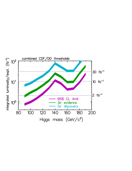
Figure 5: Tevatron Expected discovery/exclusion mass limit on the Higgs mass at the Tevatron[23])

In view of the discussions of the expected range for $m_{h}$ of the last section as well as the current LEP limits on its mass, LHC is really the collider to search for the Higgs where as Tevatron might just see some indication for it. The best mode for the detection of Higgs depends really on its mass. Due to the large value of $m_{t}$ and the large $gg$ flux at LHC, the highest production cross-section is via $gg$ fusion.

Figure 6: Expected $\sigma\cdot BR$ for different detectable SM Higgs decay modes [24].

Fig. 6[24] shows $\sigma\cdot BR$ for the SM higgs for various final states. The search prospects are optimised by exploring different channels in different mass regions. The inclusive channel using $\gamma\gamma$ final states corresponds to $\sigma\cdot BR\;{\rm of\;\;only}\>50\>fb$, but due to the low background it constitutes the cleanest channel for $m_{h}<150$ GeV. The important detector requirement for this measurement is good resolution for $\gamma\gamma$ invariant mass. The detector ATLAS at LHC should be able to achieve $\sim 1.3$ GeV whereas the detector CMS expects to get $\sim 0.7$ GeV. A much more interesting channel is production of a higgs recoiling against a jet. The signal is much lower but is also much cleaner. Use of this channel gives a significance of $\sim 5\sigma$ already at $30fb^{-1}$ for the mass range $110<m_{h}<135$ GeV. A more detailed study of the channel $pp\to h+t\bar{t}\to\gamma\gamma+t\bar{t}$ is important also for the measurement of the $ht\bar{t}$ couplings. For larger masses $(m_{h}\>\raisebox{-2.15277pt}{$\stackrel{{\scriptstyle\textstyle>}}{{\sim}}$}\>130$ GeV ) the channel $gg\to h\to ZZ^{(*)}\to 4l$ is the best channel. Fig. 6 shows that, in the range $150\>{\rm GeV}<m_{h}<190$ GeV this clean channel, however, has a rather low $(\sigma\cdot BR)$. The viability of $p\bar{p}\to WW^{(*)}\to l\bar{\nu}\bar{l}\nu$ in this range has been demonstrated[24]. Thus to summarise for $m_{h}\>\raisebox{-2.15277pt}{$\stackrel{{\scriptstyle\textstyle<}}{{\sim}}$}\>180$ GeV, there exist a large number of complementary channels whereas beyond that the gold plated $4l$ channel is the obvious choice. If the Higgs is heavier, the event rate will be too small in this channel (cf. Fig. 6). Then the best option is to tag the forward jets by studying the production of the Higgs in the process $p\bar{p}\to WWq\bar{q}\to q\bar{q}h$.

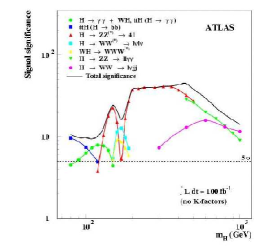
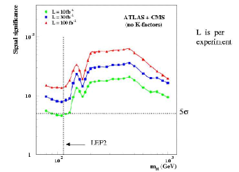
Figure 7: The expected significance level of the SM Higgs signal at LHC [25].

The figure in the left panel in fig. 7 shows the overall discovery potential of the SM higgs in all these various channels whereas the one on the right shows the same overall profile of the significance for discovery of the SM higgs, for three different luminosities, combining the data that both the detectors ATLAS and CMS will be able to obtain. The figure shows that the SM higgs boson can be discovered (i.e. signal significance $\>\raisebox{-2.15277pt}{$\stackrel{{\scriptstyle\textstyle>}}{{\sim}}$}\>5$) after about one year of operation even if $m_{h}\>\raisebox{-2.15277pt}{$\stackrel{{\scriptstyle\textstyle<}}{{\sim}}$}\>150$ GeV. Also at the end of the year the SM higgs boson can be ruled out over the entire mass range implied in the SM discussed earlier.

A combined study by CMS and ATLAS shows that a measurement of $m_{h}$ at $0.1\%$ level is possible for $m_{h}\>\raisebox{-2.15277pt}{$\stackrel{{\scriptstyle\textstyle<}}{{\sim}}$}\>500$ GeV, at the end of three years of high luminosity run and is shown in

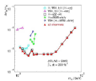
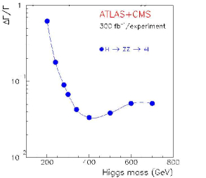
Figure 8: Expected accuracy of the measurement of Higgs mass and width at LHC[25].

fig. 8. As far as the width $\Gamma_{h}$ is concerned, a measurement is possible only for $m_{h}>200$ GeV, at a level of $\sim 5\%$ and that too at the end of three years of the high luminosity run. The values of $\Delta\Gamma/\Gamma$ that can be reached at the end of three years of high luminosity run, obtained in a combined ATLAS and CMS study, are shown in the figure in the right panel in fig. 8.

Apart from the precision measurements of the mass and the width of the Higgs particle, possible accuracy of extraction of the couplings of the Higgs with the matter and gauge particles, with a view to check the spontaneous symmetry breaking scenario, is also an important issue.

Table 2: Expected accuracy in the extraction of the Higgs couplings as evaluated by ATLAS[25].

Ratio of cross-sections	Ratio of extracted	Expected Accuracy
	Couplings	Mass Range
$\frac{\sigma(t\bar{t}h+Wh)(h\to\gamma\gamma)}{\sigma(t\bar{t}h+Wh)(h\to b\bar{b})}$	$\frac{B.R.(h\to\gamma\gamma)}{B.R.(h\to b\bar{b})}$	$\sim 15\%$, 80-120 GeV
$\frac{\sigma(h\to\gamma\gamma)}{\sigma(h\to 4l)}$	$\frac{B.R.(h\to\gamma\gamma)}{B.R.(h\to ZZ^{(*)})}$	$\sim 7\%$, 120-150 GeV
$\frac{\sigma(t\bar{t}h\to\gamma\gamma/b\bar{b})}{\sigma(Wh\to\gamma\gamma/b\bar{b})}$	$\frac{g^{2}_{ht\bar{t}}}{g^{2}_{hWW}}$	$\sim 15\%,80<m_{h}<120$ GeV
$\frac{\sigma(h\to ZZ^{*}\to 4l)}{\sigma(h\to WW^{*}\to l\nu l\nu)}$	$\frac{g^{2}_{hZZ}}{g^{2}_{hWW}}$	$\sim 10\%,130<m_{h}<190$ GeV

Table 2 shows the accuracy which would be possible in extracting ratios of various couplings, according to an analysis by the ATLAS collaboration. This analysis is done by measuring the ratios of cross-sections so that the measurement is insensitive to the theoretical uncertainties in the prediction of hadronic cross-sections. All these measurements use only the inlclusive Higgs mode.

New analyses based on an idea by Zeppenfeld and collaborators[26] have explored the use of production of the Higgs via WW/ZZ(IVB) fusion, in the process $pp\to q+q+V+V+X\to q+q+h+X.$ Here the two jets go in the forward direction. This has increased the possibility of studying the Higgs production via IVB fusion process to lower values of $m_{h}(<120{\rm GeV})$ than previously thought possible. It has been demonstrated[26] that using the production of Higgs in the process $qq\to hjj$, followed by the decay of the Higgs into various channels $\gamma\gamma,\tau^{+}\tau^{-},W^{+}W^{-}$ as well as the inclusive channels $gg\to h\gamma\gamma,gg\to h\to ZZ^{(*)}$, it should be possible to measure $\Gamma_{h},g_{hff}$ and $g_{hWW}$ to a level of $10-20\%$ , assuming that $\Gamma(h\to b\bar{b})/\Gamma(h\to\tau^{+}\tau^{-})$ has approximately the SM value. Recall, here that after a full LHC run,with a combined CMS +ATLAS analysis, the latter should be known to $\sim 15\%$. In principle, such measurements of the Higgs couplings might be an indirect way to look for the effect of physics beyond the SM. We will discuss this later.

By the start of the LHC with the possible TeV 33 run with $\int{\cal L}dt=30fb^{-1}$, Tevatron can give us an indication and a possible signal for a light Higgs, combining the information from different associated production modes: $Wh,Zh$ and $WW^{(*)}$. The inclusive channel $\gamma\gamma/4l$ which will be dominantly used at LHC is completely useless at Tevatron. So in some sense the information we get from Tevtaron/LHC will be complementary.

Thus in summary the LHC, after one year of operation should be able to see the SM higgs if it is in the mass range where the SM says it should be. Further at the end of $\sim 6$ years the ratio of various couplings of $h$ will be known within $\sim 10\%$.

Search for the SM higgs at $e^{+}e^{-}$ colliders

As discussed above LHC will certainly be able to discover the SM higgs should it exist and study its properties in some detail as shown above. It is clear, however, that one looks to the clean environment of a $e^{+}e^{-}$ collider for establishing that the Higgs particle has all the properties predicted by the SM: such as its spin, parity, its couplings to the gauge bosons and the fermions as well as the self coupling. Needless to say that this has been the focus of the discussions of the physics potential of the future linear colliders [27, 28, 29]. Eventhough we are not sure at present whether such colliders will become a reality, the technical feasibility of buliding a $500$ GeV $e^{+}e^{-}$ (and perhaps an attendant $\gamma\gamma$, $e^{-}e^{-}$ collider) and doing physics with it is now demonstrated  [27, 28, 29]. At these colliders, the production processes are $\mbox{$e^{+}e^{-}$}\to Z(^{*})h\to\ell^{+}\ell^{-}h$, called Higgstrahlung, $\mbox{$e^{+}e^{-}$}\to\nu\bar{\nu}h$ called $WW$ fusion and $\mbox{$e^{+}e^{-}$}\to t\bar{t}h$. The associated production of $h$ with a pair of stops $\tilde{t}_{1}\tilde{t}_{1}h$ also has substantial cross-sections. Detection of the Higgs at these machines is very simple if the production is kinematically allowed, as the discovery will be signalled by some very striking features of the kinematic distributions. Determination of the spin of the produced particle in this case will also be simple as the expected angular distributions will be very different for scalars with even and odd parity.

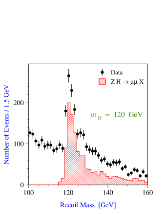
Figure 9: The $\mu^{+}\mu^{-}$ recoil mass distribution in the process $e^{+}e^{-}\rightarrow h\ Z\rightarrow X\mu^{+}\mu^{-}$ for $m_{h}$ = 120 GeV and 500 fb^-1 at $\sqrt{s}$ = 350 GeV. The dots with error bars are Monte Carlo simulation of Higgs signal and background. The shaded histogram represents the signal only [27]

.

At $\sqrt{s}=350$ GeV, a sample of $\sim$ 80,000 Higgs bosons is produced, predominantly through Higgs-strahlung, for $m_{h}=120$ GeV with an integrated luminosity of 500 fb^-1, corresponding to one to two years of running. The Higgs-strahlung process, $e^{+}e^{-}\to Zh$, with $Z\rightarrow\ell^{+}\ell^{-}$, offers a very distinctive signature (see Fig. 9) ensuring the observation of the SM Higgs boson up to the production kinematical limit independently of its decay (see Table 3). At $\sqrt{s}=500$ GeV, the Higgs-strahlung and the $WW$ fusion processes have approximately the same cross–sections, ${\cal O}$(50 fb) for 100 GeV $\>\raisebox{-2.15277pt}{$\stackrel{{\scriptstyle\textstyle<}}{{\sim}}$}\>m_{h}\>\raisebox{-2.15277pt}{$\stackrel{{\scriptstyle\textstyle<}}{{\sim}}$}\>$ 200 GeV.

Table 3: Expected number of signal events for 500 fb^-1 for the Higgs-strahlung channel with di-lepton final states $e^{+}e^{-}\rightarrow Zh\rightarrow\ell^{+}\ell^{-}X$, ($\ell=e,~{}\mu$) at different $\sqrt{s}$ values and maximum value of $m_{h}$ yielding more than 50 signal events in this final state.

$m_{h}$ (GeV)	$\sqrt{s}$ = 350 GeV	500 GeV	800 GeV
120	4670	2020	740
140	4120	1910	707
160	3560	1780	685
180	2960	1650	667
200	2320	1500	645
250	230	1110	575
Max $m_{h}$ (GeV)	258	407	639

The very accurate measurements of quantum numbers of the Higgs that will be possible at such colliders can help distinguish between the SM higgs and the lightest higgs scalar expected in the supersymmetric models. We will discuss that in the next section.

Search for the MSSM higgs at hadronic colliders

The MSSM Higgs sector is much richer and has five scalars; three neutrals: ${\cal CP}$ even h , H and ${\cal CP}$ odd A as well as the pair of charged Higgses $H^{\pm}$. So many more search channels are available. The most important aspect of the MSSM higgs, however is the upper limit[12, 13] of $130$ GeV ($200$ GeV) for MSSM (and its extensions), on the mass of lightest higgs. The masses and couplings of these scalars depend on the supersymmetric parameters $m_{A}$, the mass of the ${\cal CP}$ odd Higgs scalar $A$, the ratio of the vacuum expectation value of the two higgs fields $\tan\beta$ as well as SUSY breaking parameters $m_{\tilde{t}_{1}}$ and the mixing in the stop sector controlled essentially by $A_{t}$. In general the couplings of the h can be quite different from the SM higgs $h$; e.g. even for large $m_{A}(>400{\rm GeV}),\Gamma_{\mbox{{h}}}/\Gamma_{h}>0.8,$ over most of the range of all the other parameters. Thus such measurements can be a ‘harbinger’ of SUSY. The upper limit on the mass of h forbids its decays into a $VV$ pair and thus it is much narrower than the SM $h$. Hence the only decays that can be employed for the search of h are $b\bar{b},\gamma\gamma$ and $\tau^{+}\tau^{-}$. The $\gamma\gamma$ mode can be suppressed for the lightest supersymmetric scalar h as compared to that to $h$ in the SM. The reduction is substantial even when all the sparticles are heavy, at low $m_{A},\tan\beta$.

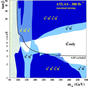
Figure 10: Number of MSSM scalars observable at LHC in different regions of $\tan\beta-m_{A}$ plane[27].

Fig. 10, taken from Ref. [27], but which is essentially a rerendering of a similar figure in Ref. [25], shows various regions in the $\tan\beta-m_{A}$ plane divided according to the number of the MSSM scalars observable at LHC, according to an ATLAS analysis, for the case of maximal mixing in the stop sector, at the end of full LHC run. This shows that for high $m_{A}(\>\raisebox{-2.15277pt}{$\stackrel{{\scriptstyle\textstyle>}}{{\sim}}$}\>200$ GeV) and low $\tan\beta(\lessapprox 8-9)$, only one of the five MSSM scalars will be observable. Furthermore, the differences in the coupling of the SM and MSSM higgs are quite small in this region. Hence, it is clear that there exists part of the $\tan\beta-m_{A}$ plane, where the LHC will not be able to see the extended Higgs sector of Supersymmetric models, even though low scale Supersymmetry might be realised.

Situation can be considerably worse if some of the sparticles, particularly $\tilde{t}$ and $\tilde{\chi}_{i}^{\pm},\tilde{\chi}_{i}^{0}$ are light. Light stop/charginos can decrease $\Gamma(\mbox{{h}}\to\gamma\gamma)$ through their contribution in the loop. For the light $\tilde{t}$ the inclusive production mode $gg\to\mbox{{h}}$ is also reduced substantially. If the channel $\mbox{{h}}\to\chi^{0}_{1}\chi^{0}_{1}$ is open, that depresses the $BR$ into the $\gamma\gamma$ channel even further[30, 31, 32, 33].

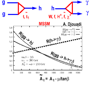
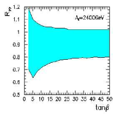
Figure 11: Effect of light sparticles on the $\gamma\gamma$ decay width and $gg$ production of the Higgs[30, 33].

The left panel in Fig. 11[30] shows the ratio

$$R(h\to\gamma\gamma)=\frac{\Gamma(\mbox{{h}}\to\gamma\gamma)}{\Gamma(h\to\gamma\gamma)}$$

and ratios $R(gg\to h),R(gg\to h\gamma\gamma)$ defined similarly. Thus we see that for low $\tan\beta$ the signal for the light neutral higgs h can be completely lost for a light stop. The panel on the right in fig. 11[33] shows $R(\mbox{{h}}\to\gamma\gamma)$ as a function of $\tan\beta$ for the case of only a light chargino and neutralino. Luckily, eventhough light sparticles, particularly a light $\tilde{t}$ can cause disappearance of this signal, associated production of the higgs h in the channel ${\tilde{t}}_{1}{\tilde{t}}^{*}_{1}\mbox{{h}}/t\bar{t}\mbox{{h}}$ provides a viable signal. However, an analysis of the optimisation of the observability of such a light stop $(m_{\tilde{t}}\simeq 100-200$ GeV) at the LHC still needs to be done.

Search for the MSSM higgs at $e^{+}e^{-}$ colliders

At an $e^{+}e^{-}$ collider with $\mbox{$\sqrt{s}$}\leq 500$ GeV, more than one of the MSSM Higgs scalar will be visible over most of the parameter space [27, 28, 29, 34, 35]. At large $m_{A}$ (which seem to be the values preferred by the current data on $b\to s\gamma$), the SM Higgs $h$ and h are indistinguishable as far as their couplings are concerned. Hence the most interesting question to ask is how well can one distinguish between the two. Recall from Fig. 10 that at the LHC there exists a largish region in the $\tan\beta-\mbox{$m_{A}$}$ plane where only the lightest h is observable if only the SM–like decays are accessible. With TESLA, the h boson can be distinguished from the SM Higgs boson through the accurate determination of its couplings and thus reveal its supersymmetric nature. This becomes clearer in the

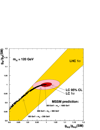
Figure 12: A comparison of the accuracy in the determination of the $g_{tt\mbox{{h}}}$ and $g_{WW\mbox{{h}}}$ Higgs couplings at the LHC and at TESLA compared to the predictions from MSSM for different values of the $m_{A}$mass [27].

Fig. 12 which shows a comparison of the accuracy of the determination of the coupling of the $h$(h) with a $WW$ and $t\bar{t}$ pair, for the LHC and TESLA along with expected values for the MSSM as a function of $m_{A}$. It is very clear that the precise and absolute measurement of all relevant Higgs boson couplings can only be performed at TESLA. The simplest way to determine the ${\cal CP}$ character of the scalar will be to produce $h$ in a $\gamma\gamma$ collider, the ideas for which are under discussion [27, 28, 29]. An unambiguous determination of the quantum numbers of the Higgs boson and the high sensitivity to ${\cal CP}$–violation possible at such machines represent a crucial test of our ideas. The measurement of the Higgs self coupling gives access to the shape of the Higgs potential. These measurements together will allow to establish the Higgs meachnism as the mechanism of electroweak symmetry breaking. To achieve this goal in its entirety a linear collider will be needed [27, 28, 29].

4 Prospects for SUSY search at colliders

The new developements in the past years in the subject have been in trying to set up strategies so as to disentangle signals due to different sparticles from each other and extract information about the SUSY breaking scale and mechanism, from the experimentally determined properties and the spectrum of the sparticles [36]. As we know, the couplings of almost all the sparticles are determined by the symmetry, except for the charginos, neutralinos and the light $\tilde{t}$. However, masses of all the sparticles are completely model dependent, as has been already discussed earlier. For $\Delta M$ = $m_{\tilde{\chi}_{1}^{\pm}}$ - $m_{\tilde{\chi}_{1}^{0}}$ $<$ 1 GeV, the phenomenology of the sparticle searches in AMSB models will be strikingly different from that in mSUGRA, MSSM etc. In the GMSB models, the LSP is gravitino and is indeed ‘light’ for the range of the values of $\sqrt{F}$ shown in Table 1. The candidate for the next lightest sparticle, the NLSP can be $\widetilde{\chi}^{0}_{1}$, $\widetilde{\tau}_{1}$ or $\widetilde{e}_{R}$ depending on model parameters. The NLSP life times and hence the decay length of the NLSP in lab is given by $L=c\tau\beta\gamma\propto\frac{1}{(M_{LSP})^{5}}$ $(\sqrt{F})^{4}$. Since the theoretically allowed values of $\sqrt{F}$ span a very wide range as shown in Table 1, so do those for the expected life time and this range is given by $10^{-4}$ $<$ c$\tau\gamma\beta$ $<$ $10^{5}$ cm. In first case the missing transverse energy ${E\!\!\!/}_{T}$ is the main signal. In the last case, along with ${E\!\!\!/}_{T}$ the final states also have photons and/or displaced vertices, stable charged particle tracks etc. as the telltale signals of SUSY [37, 38]. In view of the lower bounds on the masses of the sparticle masses established by the negative results at LEP, the most promising signal for SUSY at the run II of the Tevatron, is the pair production of a chargino-neutralino pair followed by its leptonic decay giving rise to ‘hadronically quiet’ trileptons. The reach of Tevatron run-II for this channel, in mSUGRA is shown in

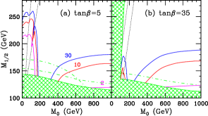
Figure 13: Expected reach of the trilepton signal at the Tevatron run-II  [39].

Fig. 13 taken from Ref. [39]. It shows the reach in the plane of mSUGRA parameters $M_{0},M_{1/2}$ for two different values of $\tan\beta$. The dash-dotted lines correspond to the limits that have been reached by the latest LEP data. The left(right) dotted lines represent where the chargino mass equals that of the $\tilde{\nu}_{\tau}(\tilde{\tau}_{R})$ for $\tan\beta=5$ and to $\tilde{\tau}_{1}(\tilde{e}_{R})$ for $\tan\beta=35$.

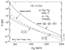
Figure 14: Expected production cross-sections for various sparticles at the LHC[40].

As is clear from the Fig. 14, LHC is best suited for the search of the strongly interacting $\tilde{g},\tilde{q}$ because they have the strongest production rates. The ${\tilde{\chi}}_{i}^{\pm},{\tilde{\chi}}^{0}_{i}$, are produced via the EW processes or the decays of the $\tilde{g},\tilde{q}$. The former mode of production gives very clear signal of ‘hadronically quiet’ events. The sleptons which can be produced mainly via the DY process have the smallest cross-section. As mentioned earlier, various sparticles can give rise to similar final states, depending on the mass hierarchy. Thus, at LHC the most complicated background to SUSY search is SUSY itself! The signals consist of events with ${E\!\!\!/}_{T}$, $m$ leptons and $n$ jets with $m,n\geq 0$. Most of the detailed simulations which address the issue of the reach of LHC for SUSY scale, have been done in the context of mSUGRA picture.

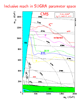
Figure 15: Expected reach for SUSY searches at the LHC[41].

We see from fig.15 that for $\tilde{g},\tilde{q}$ the reach at LHC is about $2.5$ TeV and over most of the parameter space multiple signals are observable. Note that $m_{0},m_{1/2}$ used in this figure are the same as $M_{0},M_{1/2}$ used in the text and other figures.

To determine the SUSY breaking scale $M_{SUSY}$ from the jet events, a method suggested by Hinchliffe et al[42] is used, which consists in defining

$$M_{eff}=\sum_{i=1}^{4}|P_{T(i)}|+\mbox{${E\!\!\!/}_{T}$}$$

and looking at the distribution in $M_{eff}$. The jets, that are produced by sparticle production and decay, will have $P_{T}\propto m_{1}-\frac{m_{2}^{2}}{m_{1}}$, where $m_{1},m_{2}$ are the masses of the decaying sparticles. Thus this distribution can be used to determine $M_{SUSY}$.

Figure 16: Determination of SUSY breaking scale using jet events at LHC point [42].

The distribution in fig. 16 shows that indeed there is a shoulder above the SM background. The scale $M_{SUSY}$ is defined either from the peak position or the point where the signal is aprroximately equal to the background. Then of course one checks how well $M_{SUSY}$ so determined tracks the input scale. A high degree of correlation was observed in the analysis, implying that this can be a way to determine the SUSY breaking scale in a precise manner.

It is possible to reconstruct the masses of the charginos/neutralinos using kinematic distributions.

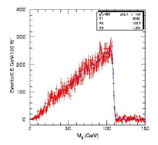
Figure 17: Kinematic reconstruction of the mass of ${\tilde{\chi}}_{2}^{0}$ from the dilepton mass distribution [41].

Fig. 17 demonstrates this, using the distribution in the invariant mass $m_{l^{+}l^{-}}$ for the $l^{+}l^{-}$ pair produced in the decay ${\tilde{\chi}}^{0}_{2}\to{\tilde{\chi}}_{1}^{0}l^{+}l^{-}$. The end point of this distribution is $\sim m_{{\tilde{\chi}}_{2}^{0}}-m_{{\tilde{\chi}}_{1}^{0}}$. However, such analyses have to be performed with caution. As pointed out by Nojiri et al[43], the shape of the spectrum near the end point can at times depend very strongly on the dynamics such as the composition of the neutralino and the slepton mass. One can still use these determinations to extract model parameters, but one has to be careful.

Studies of SUSY and SUSY breaking scale at the $e^{+}e^{-}$ colliders

At the $e^{+}e^{-}$ colliders one can study with great accuracy the production of sleptons, squarks, charginos and neutralinos. The precision measurements of the sparticle masses and quantum numbers allows testing the basic predictions of supersymmetry about the particle spectrum. There have been a large number of dedicated studies of the possibilities of precision measurements of the properties of these sparticles at the next generation of Linear Colliders [44, 45, 46]. Study of the third generation of sfermions are shown to yield particularly interesting information about SUSY models. Almost no study is possible without use of polarisation, at least for one of the initial state fermions.

Sleptons and Charginos/Neutralinos

The masses of sleptons can be determined at an LC essentially using kinematics. Making use of partial information from the LHC, it will be possible to tune the energy of the LC to produce the sfermions sequentially. The pair produced lightest sleptons will decay through a two body decay. Let us take the example of $\widetilde{\mu}_{R}$ which will have the simplest decay. So one has in this case,

$$e^{+}e^{-}\rightarrow\widetilde{\mu}_{R}\widetilde{\mu}_{R}^{*}\rightarrow\mu^{+}\mu^{-}\tilde{\chi}_{1}^{0}\tilde{\chi}_{1}^{0}$$

Since the slepton is a scalar the decay energy distribution for the $\mu$ produced in two body decay of $\widetilde{\mu}_{R}$, will be flat with

$${m_{\widetilde{\mu}_{R}}\over 2}\left(1-{{m_{\widetilde{\chi}^{0}_{1}}^{2}}\over{m_{\widetilde{\mu}_{R}}^{2}}}\right)\gamma(1-\beta)<E_{\mu}<{m_{\widetilde{\mu}_{R}}\over 2}\left(1-{{m_{\widetilde{\chi}^{0}_{1}}^{2}}\over{m_{\widetilde{\mu}_{R}}^{2}}}\right)\gamma(1+\beta).$$

Thus measuring the end points of the $E_{\mu}$ spectrum accurately will yield a precision measurement of the masses $m_{\widetilde{\mu}_{R}}$, $m_{\widetilde{\chi}^{0}_{1}}$ [27, 28, 29]. However, the method of using the end point of the energy spectrum will not work so well for the third generation slepton, e.g. , for $\widetilde{\tau}_{1}\widetilde{\tau}_{1}^{*}$ production and decay  [47, 48].

Another method for precision determination of the masses of the sleptons and the lighter charginos/neutralinos, is to perform threshold scan. The linear $\beta$ dependence as opposed to the $\beta^{3}$ dependence of the cross-section, near the threshold (where $\beta$ is the c.m. velocity of the produced sparticle) makes the method more effective for the spin 1/2 charginos/neutralinos than the sleptons. The threshold scans offer the possibility of very accurate mass determinations [27] of the sparticles, albeit with very high luminosity.

Recent analyses of the mass determination of $\widetilde{\tau}_{1}$  and ${\widetilde{\nu}}_{\tau_{1}}$ [48] using the continuum production, show that only an accuracy of $\sim 2\%$ for $m_{\widetilde{\tau}_{1}}$ (consistent with the earlier analyses [47]) and even much worse $6-10\%$ for $m_{\widetilde{\nu}_{\tau}}$, is possible even after a use of optimal polarisation and comparable luninosities as in the threshold scan case. A recent study [49] addressing these issues indicates that threshold scans may not be the optimal way to measure the masses for the second and third generation sleptons. This is caused by the low rates which force one to go away from the threshold and also the ‘a priori’ unknown branching ratios of the $\widetilde{\tau}_{1}$ or $\widetilde{\nu}_{\tau}$. It is very important to clearly understand just how well these measurements can be made, as these accuracies affect, crucially, the projected abilities to glean information about the SUSY breaking scale.

Squarks

Clearly squarks are the only strongly interacting particles about whom direct information can be obtained at the $e^{+}e^{-}$ collider. For the strongly interacting sfermions (squarks) the decay is $\widetilde{q}\to q\widetilde{\chi}^{0}_{1}$. As a result, one has to study the end point of the distribution in $E_{jet}$. The hadronization effects can in principle deteriorate the accuracy of the determination of $m_{\widetilde{q}}$. An alternate estimator  [50] of $m_{\tilde{q}}$ is the peak of the distribution in the minimum kinematically allowed mass of the $q\widetilde{\chi}^{0}_{1}$ system produced in

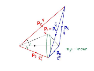
Figure 18: Determination of the minimum kinematically allowed squark mass, following Ref. [50].

$\tilde{q}$ decay; $m_{\tilde{q},min}$. The minimum squark mass corresponds to maximum possible $|\vec{p}_{4}|$ and can be easily determined following the construction in Fig. 18. The figure in the left panel of Fig. 19, taken from Ref. [50] shows the efficacy of this estimator for a 500 GeV machine with $10$ fb^-1 luminosity per polarisation, the latter

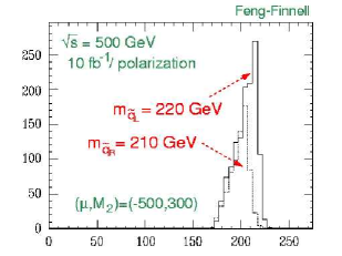
Figure 19: Accuracy of determination of $m_{\widetilde{q}}$ using the $m_{\widetilde{q},min}$ defined in [50].

being used for separating $\widetilde{q}_{L}/\widetilde{q}_{R}$ contributions, for a particular point in the MSSM parameter space. Figure in the right panel shows that this variable provides a good estimate of $m_{\widetilde{q}}$ even after radiative corrections, both in production and decay, have been included [51].

If the squarks are lighter than the glunios, any information on gluino masses at an $e^{+}e^{-}$ collider can only come from the assumed relations between the masses of the electroweak and strong gauginos.

Precision determination of mixings

The mixing between various interaction eigenstates in the gaugino sector as well as the, in general, large mixing in the L-R sector for the third generation squarks and sleptons, is decided respectively by $M_{1},M_{2},\mu,\tan\beta$ and $\mu,\tan\beta,A$ as well as various scalar mass parameters. So clearly an accurate measurement of these mixings along with the precision measurements of masses offers further clues to physics at high scale.

Possibilities of the determination of L-R mixing in the third generation sfermions have been investigated [27, 28, 29]. The mass eigenstates can be written down in terms of the interaction eigenstates for, e.g. , staus as $\widetilde{\tau}_{1}=\widetilde{\tau}_{L}\cos\theta_{\tau}+\widetilde{\tau}_{R}\sin\theta_{\tau}$,$\widetilde{\tau}_{2}=\widetilde{\tau}_{L}\sin\theta_{\tau}+\widetilde{\tau}_{R}\cos\theta_{\tau}$. It is clear that polarised $e^{-}$/$e^{+}$ beams can play a crucial role in determining $\theta_{\tau}$. Let us, for example, consider $e^{+}e^{-}\to\widetilde{\tau}_{1}\widetilde{\tau}_{1}^{*}$. Further let us consider the case of 100 % polarisation in particular. The pair production proceeds through an exchange of $\gamma$/Z in $s$-channel. For energies $\sqrt{s}$ $>$ $>$ $m_{Z}$, with $P_{e^{-}}$ = 1, one can essentially interpret this $s$-channel exchange of $\gamma$/Z as an U(1) gauge boson, $B$. In this limit $\sigma(\widetilde{\tau}_{R})$ = 4 $\sigma(\widetilde{\tau}_{L})$. Thus it is clear that a measurement of $\sigma(e^{+}e^{-}\to\widetilde{\tau}_{1}^{*}\widetilde{\tau}_{1})$ along with a knowledge of polarisation of $e^{-}$ beam can lead to an extraction of $\cos\theta_{\tau}$. Further the polarisation of $\tau$ produced in $\widetilde{\tau}_{1}$ decay provides a measurement of the mixing angle in the neutralino sector as well [52]. Let us consider $\widetilde{\tau}_{R}\to\tau\widetilde{\chi}^{0}_{1}$ depicted in Fig. 20. The $\tilde{B}$ component of $\widetilde{\chi}^{0}_{1}$ produces $\widetilde{\tau}_{R}$, whereas the higgsino

Figure 20: $\widetilde{\tau}_{R}\to\tau\widetilde{\chi}^{0}_{1}$.

component will flip the chirality and produce $\widetilde{\tau}_{L}$. Thus the measurement of $\widetilde{\tau}_{1}^{*}\widetilde{\tau}_{1}$ production with polarised $e^{-}$ beams and the polarisation of decay $\tau^{s}$ can give very useful information on both the mixings: the $L-R$ mixing in the stau sector and the mixing in the neutralino sector. The $\tau$ polarisation can be measured by looking at the energy distribution of the decay product $\rho$ in the hadronic decay of $\tau$ [52].

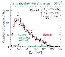
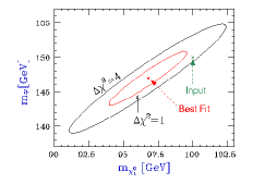
Figure 21: Precision of the determination of $m_{\widetilde{\tau}_{1}}$ and $m_{\widetilde{\chi}^{0}_{1}}$ for luminosities and polarisation mentioned in the figure. Taken from Ref.[47].

Fig. 21 [47] shows the possible accuracy of a simultaneous determination of $m_{\tilde{\tau_{1}}}$ - $m_{\tilde{\chi_{1}^{0}}}$ from the determination of the end points of the energy spectrum, for $\int{\cal L}dt=100\ {\rm fb}^{-1},P_{e^{-}}=0.95$ and $\sqrt{s}=500$ GeV. The input value lies outside the $\Delta\chi^{2}$ = 1 contour around the best fit value. However, if $m_{\widetilde{\chi}^{0}_{1}}$ is assumed to be known, then $\Delta m_{\widetilde{\tau}_{1}}$ goes down considerably and a 1-2% determination at $1\sigma$ level is possible.

A study of the chargino sector at the LC can provide a precision determination of the higgsino-gaugino mixing and consequently an accurate determination of all the Lagrangian parameters which dictate the properties of the chargino sector [53, 54, 55, 27, 28]. This requires, along with the determination of $m_{\widetilde{\chi}^{\pm}_{1}},m_{\widetilde{\chi}^{0}_{1}}$ and $\sigma^{\rm tot}_{\widetilde{\chi}^{+}_{1},\widetilde{\chi}^{-}_{1}}$, a study of either the dependence of the production cross-section on the initial beam polarisations or the polarisation of the produced charginos through the angular distribution of their decay products. Since $\sigma(e^{+}e^{-}\to\widetilde{\chi}^{-}_{i}\widetilde{\chi}^{+}_{j})$ depends on $m_{\widetilde{\nu}}$, its knowledge is also necessary. This can be obtained by studying the energy dependence of the $\sigma^{\rm tot}$, even if $m_{\widetilde{\nu}}$ is beyond the kinematic range of the collider. If only the lightest chargino is available kinematically, then one can determine the mixing angles in the chargino sector $\Phi_{L},\Phi_{R}$ defined through

$$\widetilde{\chi}^{-}_{1L}=\cos\Phi_{L}\tilde{W}^{-}_{L}+\sin\Phi_{L}\tilde{H}^{-}_{2L},\widetilde{\chi}^{-}_{1R}=\cos\Phi_{R}\tilde{W}^{-}_{R}+\sin\Phi_{R}\tilde{H}^{-}_{1R},$$ (5)

only upto a two fold ambiguity. However, this can be removed, using the information on the transverse polarisation, as shown in Fig. 22. If both the charginos are accessible kinematically, $\cos 2\Phi_{R},\cos 2\Phi_{L}$ can be determined uniquely through measurements of $\sigma_{L/R}(\widetilde{\chi}^{+}_{i}\widetilde{\chi}^{-}_{j})$, as shown in the lower panel

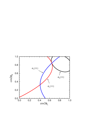
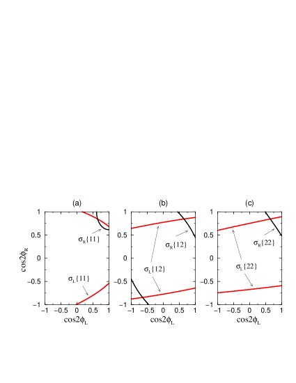
Figure 22: Demonstration of unique determination of mixing angles in the chargino sector using polarised beams [55].

of the same figure. It has been shown, in a purely theoretical study  [55], in the context of TESLA, using only statistical errors, that with $\int{\cal L}dt=1\ ab^{-1},\cos 2\Phi_{L},\cos 2\Phi_{R}$ can be determined to an accuracy of $\sim 1-3\%$. Along with the information on $m_{\widetilde{\chi}^{+}_{i}}$ the mixing angles can then lead to an unambiguious determination of the Lagrangian parameters $M_{2},\mu$ and $\tan\beta$. However, since all the variables are proportional only to $\cos 2\beta$, the accuracy of $\tan\beta$ determination is rather poor at high $\tan\beta$. At high $\tan\beta$, measurements in the slepton sector (stau/selectron) discussed earlier [47] afford a better determination.

Above discussion already shows how an efficient use of polarisation of both $e^{+}/e^{-}$ beams, allows a high precision determination of the mixings among the $L-R$ sfermions as well as in the gaugino-higgsino sector. This is, indeed, indirectly a determination of the hypercharges of the various sparticles. It has been demonstrated [54], using realistic simulation of the backgrounds, that it is possible to reconstruct the $\widetilde{\mu}$ angular distribution in the process $e^{+}e^{-}\to\widetilde{\mu}\widetilde{\mu}^{*}\to\mu^{+}\mu^{-}+E_{T}/\;\>$   and hence determine the spin of the smuon with precision. Further, the cross-section of $\widetilde{e}_{R}\widetilde{e}_{R}^{*}$ production can be used as a very sensitive probe of the equality of the couplings $g_{\widetilde{e}e_{R}\tilde{B}}$ and $g_{eeB}$. This is due the contribution of the $t$ channel diagram shown in the left-hand panel of Fig. 23, which involves a $\widetilde{\chi}^{0}_{i}$ exchange. The contribution

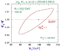
Figure 23: Simultaneous determination of $M_{1}$ and $g_{\widetilde{e}_{R}e\widetilde{B}}$, in a study of $\widetilde{e}_{R}\widetilde{e}_{R}^{*}$ production.

to the production cross-section of the $\widetilde{e}_{R}\widetilde{e}_{R}^{*}$ pair is sensitive to the bino component of $\widetilde{\chi}^{0}_{i}$ and hence to the $U(1)$ gaugino mass parameter $M_{1}$ and the coupling $g_{\widetilde{e}_{R}e_{R}B}$. At tree level we expect, due to supersymmetry,

$$g_{\tilde{e}_{R}e_{R}\tilde{B}}=g_{eeB}=\sqrt{2}g_{2}\tan\theta_{W}=\sqrt{2}g_{1}Y_{b}=g_{Y}.$$ (6)

Using $\sigma(e^{+}e^{-}\to\widetilde{e}_{R}\widetilde{e}_{R}^{*})$ and $\frac{d\sigma}{d\cos\theta}(e^{+}e^{-}\to\widetilde{e}_{R}\widetilde{e}_{R}^{*})$, one can determine $g_{\widetilde{e}_{R}e_{R}\tilde{B}}$ and $M_{1}$ simultaneously. For an integrated luminosity of $100\ {\rm fb}^{-1}$, $Y_{b}$ of Eq. 6 can be determined to an accuracy of $1\%$ [47]. This is shown in the right panel of Fig. 23. This expected accuracy is actually comparable to the size of the SUSY radiative corrections [56] to the tree level equality of Eq. 6 and hence this measurement can serve as an indirect probe of the mass of the heavy sparticles.

The precision measurements of the masses and the mixings in the sfermion and the chargino/neutralino sector at the LC will certainly allow to establish existence of supersymmetry as a dynamical symmetry of particle interactions. However, this is not all these measurements can achieve. The high precision of these measurements will then allow us to infer about the SUSY breaking scale and the values of the SUSY breaking parameters at this high scale, just the same way the high precision measurements of the couplings $g_{1},g_{2}$ and $g_{3}$ can be used to get a glimpse of the physics of unification and its scale.

There are essentially two different approaches to these studies. In the pioneering studies  [54, 47], the JLC group investigated how accurately one can determine the parameters $M_{1},M_{2},\mu,\tan\beta$ and $M_{0}$ at the high scale by fitting these directly to the various experimental observables such as the polarisation dependent production cross-sections of the sparticles, angular distributions of the decay products etc., that have been mentioned in the discussion so far.

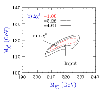
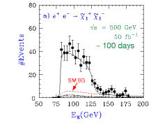
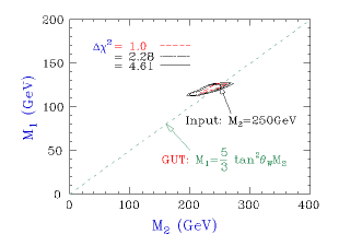
Figure 24: Simultaneous determination of chargino/neutralino mass from chargino studies and consequent testing of the GUT relation between $M_{1}$ and $M_{2}$ [54].

An example of this is shown in Fig. 24. The right hand figure in the top panel shows how a determination of the energy distribution of the ‘W’ produced in the decay of $\widetilde{\chi}^{+}/\widetilde{\chi}^{-}$, in the reaction $e^{+}e^{-}\to\widetilde{\chi}^{+}_{1}\widetilde{\chi}^{-}_{1}$, affords a determination of $m_{\widetilde{\chi}^{0}_{1}}$ and $m_{\widetilde{\chi}^{\pm}}$ shown in the left panel. The lower panel then shows how using the masses $m_{\widetilde{\chi}^{\pm}},m_{\widetilde{\chi}^{0}_{1}}$ along with $\sigma_{R}(\widetilde{\chi}^{\mp}_{1}),\sigma_{R}(\tilde{e}_{R})$ and the angular distribution of the decay leptons one can extract $M_{1},M_{2}$ at the GUT scale and test the GUT relation.

A different approach [27] is to use the experimental observables such as cross-sections, angular distributions to determine the physical parameters of the system such as masses and mixings and then use these to determine the Lagrangian parameters $M_{1},M_{2},\mu,\tan\beta$ at the EW scale itself. Thus the possible errors of measurements of the experimental quantities alone will control the accuracy of the detrmination of these parameters. There are again two ways in which this information can be used: one is a top down approach which in spirit is similar to the earlier one as now one uses these accurately determined Lagrangian parameters at the EW scale to fit their values at the high scale and then compare them with the input value.

A completely different and a very interesting way of using the information on these masses [57] is the bottom up approach where, one starts with these Lagrangian parameters extracted at the weak scale and use the renormalisation group evolution (RGE) to calculate these parameters at the high scale. As explained in the introduction, different SUSY breaking mechanisms differ in their predictions for relations among these various parameters at the high scale. The ineteresting aspect of the bottom up approach is the possibility they offer of testing these relations ‘directly’ by reconstructing them from their low energy values using the RGE. In the analysis the ‘experimental’ values of the various sparticle masses are generated in a given scenario (mSUGRA,GMSB etc.) starting from the universal parameters at the high scale appropriate for the model under consideration and using the evolution from the high scale to the EW scale. These quantities are then endowed with experimental errors expected to be reached in the combined analyses from LHC and an LC with energy upto $1$ TeV , with an integrated luminosity of $1{\rm ab}^{-1}$. Then these values are evloved once again to the high scale. The figure in the left panel of Fig. 25

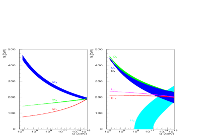
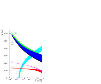
Figure 25: Bottom up approach of the determination of the sparticle mass parameters for mSUGRA and GMSB[57]. Values of the model parameters as given there.

shows results of such an exercise for the gaugino and sfermion masses for the mSUGRA case and the one on the right for sfermion masses in GMSB. The width of the bands indicates $95\%$ C.L. Bear in mind that such accuracies will require a 10-20 year program at an LC with $\sqrt{s}\leq 1.5$ TeV. The two figures in the left panel show that with the projected accuracies of measurements, the unification of the gaugino masses will be indeed demonstrated very clearly.

All these discussions assume that most of the sparticle spectrum will be accessible jointly between the LHC and a TeV energy LC. If however, the squarks are superheavy [15, 58] (a possibility allowed by models) then perhaps the only clue to their existence can be obtained through the analogue of precision measurements of the oblique correction to the SM parameters at the Z pole. These superoblique corrections [56], modify the equalities between various couplings mentioned already in Eq. 6. These modifications arise if there is a large mass splitting between the sleptons and the squarks. The expected radiative corrections imply

$${{\delta g_{Y}}\over g_{Y}}\simeq{{11g_{Y}^{2}}\over{48\pi^{2}}}ln\left({m_{\widetilde{q}}}\over{m_{\tilde{l}}}\right).$$

Thus if the mass splitting is a factor 10 one expects a deviation from the tree level relation by about $0.7\%$. The discussions of the earlier section demonstrate that it might be possible at an LC to make such a measurement.

5 Exploring the ‘SUSY’less option at Colliders

In the introduction we saw that apart from the option of elementary higgs and SUSY there exist also two other options to handle the hierarchy problems; viz. the composite scalars [9] and extra ’large’ dimensions; warped or otherwise  [21, 22]. We argued that in the former case one will see evidence of deviation of the trilnear and quartic gauge boson couplings from the SM predictions.

Figure 26: Comparison of limits on the chiral Lagrangian parameters $L_{9}$ at the future colliders, from[9].

Fig. 26 taken from Ref. [9] shows an example of the reach for the particular operator $L_{9}$ at the LHC and the planned $e^{+}e^{-}$  $\gamma\gamma$ colliders.

The whole development of the subject of ‘large’ extra dimensions at LHC is a very good example as to how the various features of the detectors, such as good lepton detection, can be used very effectively in looking for ‘new’ physics which was not taken into account while designing the detector. In the context of LHC, the clearest signal for these ‘large’ dimensions is via the observation of graviton resonances[59] in the dilepton spectrum via the process $gg\to G\to l^{+}l^{-}$. It has been demonstrated by Hewett et al[59] that by using the constraints already available from the dijet/dilepton data from the Tevatron and making reasonable assumptions so that the EW scale is free from hierarchy problem, in the scenario with ‘warped’ extra dimesnions[21], the parameter space of the model can be completely covered at LHC using the dilepton channel.

Apart from determining the mass of the graviton, it is also essntial to check the spin of the exchanged particle. ATLAS performed an analysis[60], which showed that the acceptance of the detector is quite low at large $\cos\theta^{*}$.

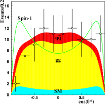
Figure 27: Angular distribution in the cm. frame for the $l^{+}l^{-}$ pair expected in the detector for the graviton along with the expectation for a spin 1 particle at LHC[60].

The left panel of fig. 27 shows the different angular distributions expected for different spin exchanges. For the spin-2 case the contributions from the $gg$ and $qq$ initial state are shown separately. The panel on the right shows that even with the lowered acceptance, it might be possible to discriminate against a spin-1 case. Many more investigations on the subject are going on and the end conclusion is that it should be possible to see the effect of these ‘large’ compact dimensions (warped or otherwise) at the LHC upto almost all the values of the model parameters which seem reasonable and for which the theoretical formulation remains consistent.

The effects of these ’large’ extra dimensions can be studied at the $e^{+}e^{-}$ and $\gamma\gamma$ colliders very easily, the available polarisation serving a very useful role [61, 62, 27, 28, 29]. Studies of large $p_{T}$ jet production, $t\bar{t}$ pair production, fermion pair production can see these ‘extra’ large dimensions if they correpsond to the TeV scale which should be the scale at which they should appear if they have to obviate the need of SUSY to solve the hierarchy problem. The joint reach of the LHC and the next linear colliders will certainly cover that range.

6 Conclusion

In conclusion we can say that the TeV energy colliders, both hadronic and leptonic, are necessary to further our understanding of the fundamental particles and interactions among them and that such colliders will definitely be able to provide further answers to this very basic question that we ask. Such colliders should 1)either be able to find a fundamental higgs scalar, study its properties in detail to test whether it is the SM higgs and 2) obtain evidence for existence of Supersymmetry (which seems necessary for the theoretical consistency of the SM) if nature has chosen the supersymmetric path and obtain information about the Supersymmetry breaking and breaking scale. 3) Alternatively they should be able to find evidence for some other physics beyond the SM such as composite scalars or the extra ‘large’ dimensions which do not need the existence of supersymmetry to solve the hierarchy problem. In any situation the physics prospects of the currently running colliders like the Tevatron, future collider like the LHC which is now under preparation and the linear $e^{+}e^{-}$, $\gamma\gamma$ colliders which are in the planning stages are extremely exciting and hold a lot of promise to help us understand some very basic issues about the elementary particles and their interactions.

References

-
[1]
The LEP Electroweak Working Group,
http://lepewwg.web.cern.ch/LEPWWG/seminar/. - [2] H.N. Brown et al., Muon g-2 Collaboration, Phys. Rev. Lett. 86, 2227r (2001), hep-ex/0102017.
- [3] J. M. Cornwall, D. N. Levin and G. Tiktopoulos, Phys. Rev. Lett. 30 (1973) 1268. [Erratum-ibid 31 (1973) 572]; Phys. Rev. D 10, 1145 (1974) [Erratum-ibid. D 11, 972 (1974)].
- [4] F. Boudjema, hep-ph/0105040.
- [5] B. W. Lee, C. Quigg and H. B. Thacker, Phys. Rev. D 16, 1519 (1977).
- [6] T. Hambye and K. Riesselmann, Phys. Rev. D 55, 7255 (1997); hep-ph/9708416 in ECFA/DESY study on particles and detectors for for the linear colliders, Ed. R. Settlers, DESY 97-123E.
- [7] H. Murayama and C. Kolda, Journal of High Energy Physics 7, 35 (2000).
- [8] R. Barbieri and A. Strumia, Phys. Lett. B 462, 144 (1999), hep-ph/0005203, hep-ph/0007265.
- [9] F. Boudjema, Invited talk at the Workshop on Physics and Experiments with Linear Colliders, Morioka, Japan, 1995, eds. A. Miyamoto et al.,, World Scientific, 1996, p. 199.
- [10] M. Peskin and T. Takeuchi, Phys. Rev. Lett. 65, ( (1)990) 964. G. Altarelli and R. Barbieri Phys. Lett. B 253, ( (1)991) 161.
- [11] R. Kaul, Phys. Lett. B 109, ( (1)982) 19.
- [12] S. Heinemeyer, W. Hollik and G. Weiglein, Phys. Lett. B 455, 179 (1999); Eur. Phys. J. C 9, 343 (1999); R. J. Zhang, PLB 447, 89 (1999), J.R. Espinoza and R.J. Zhang, JHEP 3, 26 (2000), hep-ph/0003246; M. Carena, H.E. Haber, S. Heinemeyer, W. Hollik, C.E.M. Wagner and G. Weiglein, Nucl. Phys. B 580, 29 (2000).
- [13] J.R. Espinoza and M. Quiros, Phys. Rev. Lett. 81, 516 (1998).
- [14] Barbieri, R., and Giudice, G.F., Nucl. Phys. B 306, 63 (1988).
- [15] Feng, J.L, Matchev, K.T., and Moroi, T., Phys. Rev.Lett. 84, 2322 (2000), hep-ph/9908309; Feng, J.L., and Moroi, T., Phys. Rev. D 61, 095004 (2000), hep-ph/9907319.
- [16] Randall, L., and Sundrum, R., Nucl. Phys. B 557, 79 (1999), hep-th/9810155.
- [17] Giudice, G.F., Luty, M.A., Murayama, H., and Rattazi, R., JHEP 27, 9812 (1998), hep-ph/9810442.
- [18] Dine, M., Nelson, A.E., and Shirman, Y., Phys. Rev. D 51, 1362 (1995), hep-ph/9408384; Dine, M., Nelson, A.E., Nir, Y., and Shirman, Y., Phys. Rev. D 53, 2658 (1996), hep-ph/9507378.
- [19] Schmaltz, M., and Skiba, W., Phys. Rev. D 62, 095004 (2000), hep-ph/0004210; Phys. Rev. D 62, 095005 (2000), hep-ph/0001172; Chacko, Z., Luty, M.A., Nelson, A.E., and Ponton, E., JHEP 1, 3 (2000), hep-ph/9911323.
- [20] Peskin, M. E., hep-ph/0002041, Concluding lecture at the International Europhysics Conference on High Energy Physics, July 1999, Tampere, Finland.
- [21] L. Randall and R. Sundrum, Phys. Rev. Lett. 83, 3370 (1999), ibid., 4690 (1999).
- [22] N. Arkani-Hamed, S. Dimoupoulos and G. Dvali, Phys. Lett. B 429, 263 (1998),Phys. Rev. D 59, 086004 (1999); I. Antoniadis, N. Arkani-Hamed, S. Dimopoulous and G. Dvali, Phys. Lett. B 436, 257 (1998).
- [23] M. Carena et al., “Report of the Tevatron Higgs working group,” hep-ph/0010338.
- [24] M. Dittmar, Pramana 55, 151 (2000).
- [25] F. Gianotti, Talk presented at LHCC meeting, http://gianotti.home.cern.ch/gianotti/phys_info.html, F. Gianotti and M. Pepe Altarelli, hep-ph/0006016.
- [26] For a nice summary, see, D. Zeppenfeld, hep-ph 0005151.
- [27] J. A. Aguilar-Saavedra et al. [ECFA/DESY LC Physics Working Group Collaboration], hep-ph/0106315.
- [28] T. Abe et al. [American Linear Collider Working Group Collaboration], SLAC-R-570 Resource book for Snowmass 2001, 30 Jun - 21 Jul 2001, Snowmass, Colorado.
- [29] ACFA Linear Collider Working Group report:, hep-ph/0109166, available at url http://acfaghep.kek.jp/acfareport.
- [30] A. Djouadi, Phys. Lett. B 435, 1998 (101).
- [31] A. Djouadi, hep-ph 9903382.
- [32] G.Belanger, F. Boudjema and K. Sridhar, Nucl. Phys. B 568, 3 (2000).
- [33] G. Belanger, F. Boudjema, F. Donato, R. Godbole and S. Rosier-Lees, Nucl. Phys. B 581, 3 (2000).
- [34] M. Spira and P.M. Zerwas, Lectures at the Internationale Universitätwochen für Kern und Teilchen Physik, hep-ph/9803257 and references therein.
- [35] A. Djouadi, hep-ph 9910449.
- [36] For a summary of the recent developements, see for example, R.M. Godbole, hep-ph/0011237, In Proceedings of the 8th Asia Pacific Physics Conference, Taipei, Taiwan, Aug. 2000; R. M. Godbole, hep-ph/0102191, In Proceedings of the Linear Collider Workshop, LCWS00, Fermilab, U.S.A. Oct. 2000.
- [37] S. Abel et al. “Report of the SUGRA working group for run II of the Tevatron,” hep-ph/0003154; R. Culbertson et al., “Low-scale and gauge-mediated supersymmetry breaking at the Fermilab Tevatron Run II,” hep-ph/0008070.
- [38] For a comrpehensive discussion of the LHC capabilities for SUSY, see for example, ATLAS Technical Design Report 15, CERN/LHCC/99-14 and 15 (1999).
- [39] K. T. Matchev and D. M. Pierce, Phys. Lett. B 467, 225 (1999)
- [40] H. Baer, C. Chen, F. Paige and X. Tata, Phys. Rev. D 53, 6241 (1996).
- [41] G. Polesello, Talk presented at the SUSY2K, June 2000, http://wwwth.cern.ch/susy2k/susy2kfinalprog.html.
- [42] I. Hinchliffe, F.E. Paige, M.D. Shapiro, J. Soderqvist and W. Yao, Phys. Rev. D 55, 5520 (1997).
- [43] M. M. Nojiri and Y. Yamada, Phys. Rev. D 60, 015006 (1999).
- [44] Peskin M.E. Prog. Theor. Phys. Supplement 123, 507 (1996), hep-ph/9604339; Murayama, H., and Peskin, M.E., Ann. Rev. Nuc. Part. Sci. 46, 533 (1996); hep-ex/9606003.
- [45] Zerwas, P.M., Surv. High Energy Physics 12, 209 (1998).
- [46] For a recent summary see, Refs. [27, 28, 29] and references therein.
- [47] Nojiri, M.M., Fujii, K., and Tsukamoto, T., Phys. Rev. D 54, 6756 (1996), hep-ph/9606370.
- [48] Baer, H., Balázs, C., Mizukoshi, J.K., and Tata, X., Phys. Rev. D 63, 055011 (2001), hep-ph/0010068,
- [49] J. K. Mizukoshi, H. Baer, A. S. Belyaev and X. Tata, hep-ph/0107216.
- [50] Feng, J. L., and Finnell, D.E., Phys. Rev. D 49, 2369 (1994), hep-ph/9310211.
- [51] Drees, M., Eboli, O.J.P., Godbole, R.M., and Kraml, S., hep-ph/0005142, In SUSY working group report, Physics at TeV colliders (Les Houches), http://lappc-th8.in2p3.fr/Houches99/susygroup.html.
- [52] Nojiri, M.M., Phys. Rev. D 51, 6281 (1995), hep-ph/9412374.
- [53] Tsukamoto, T., Fujii, K., Murayama, H., Yamaguchi, M., and Okada, Y., Phys. Rev. D 51, 3153 (1995).
- [54] Feng, J.L., Murayama, H., Peskin, M.E., and Tata, X., Phys. Rev. D 52, 1418 (1995), hep-ph/9502260.
- [55] Choi, S.Y., Djouadi, A., Guchait, M., Kalinowski, J., Song, H.S., and Zerwas, P.M., Eur. Phys. J C 14, 535 (2000), hep-ph/0002033.
- [56] Nojiri, M.M., Pierce, D.M, and Yamada, Y., Phys. Rev. D 57, 1539 (1998), hep-ph/9707244; Cheng, H.C., Feng, J.L., and Polonsky, N., Phys. Rev. D 57, 152 (1998), hep-ph/9706476; Katz, E., Randall, L., and Su, S., Nucl. Phys. B 536, 3 (1998), hep-ph/9801416.
- [57] Blair, G.A., Porod, W., and Zerwas, P.M., Phys. Rev. D 63, 017703 (2001), hep-ph/0007107.
- [58] Bagger, J.A., Feng J.L, Polonsky, N. and Zhang, Ren-Jie, Phys. Lett. B 473, 264 (2000), hep-ph/9911255; Bagger, J.A., Feng, J.L., and Polonsky, N., Nucl. Phys. B 563, 3 (1999), hep-ph/9905292.
- [59] H. Davoudiasl, J.L. Hewett and T.Rizzo, Phys. Lett. B 473, 49 (2000), Phys. Rev. Lett. 84, 2080 (2000), hep-ph/0006041.
- [60] B. C. Allanach, K. Odagiri, M.A. Parker and B.R. Webber, Journal of High Energy Physics 9, 019 (2000).
- [61] R. M. Godbole, hep-ph/0011236.
- [62] K. Sridhar, Int. J. Mod. Phys. A 15, 2397 (2000), hep-ph/0004053 .