CERN-TH/2002-034

HIP-2002-06/TH

Gravitational decays of heavy particles
in large extra dimensions

 

Abstract

In the framework of quantum gravity propagating in large extra dimensions, we analyze the inclusive radiative emission of Kaluza-Klein spin-2 gravitons in the two-fermions decays of massive gauge bosons, heavy quarks, Higgs bosons, and in the two-massive gauge bosons decay of Higgs bosons. We provide analytical expressions for the square modulus of amplitudes summed over polarizations, and numerical results for the widths and branching ratios. The corresponding decays in the $Z$, top quark, and Higgs boson sectors of the standard model are analyzed in the light of present and future experiments.

 

1 Introduction

After the recent proposal of Arkani–Hamed, Dimopoulos, and Dvali (ADD) on quantum gravity propagating in large extra dimensions [1], there has been an intense theoretical activity on this subject [2]-[6]. In [1], it was pointed out that if compactified extra dimensions exist, with only gravity propagating in the bulk and standard matter with gauge fields confined in the usual 3+1 dimensional space, then the fundamental scale of quantum gravity could be much lower than the Planck scale $M_{P}$. In particular the weakness of gravity might be due to the large size of the compactified extra dimensional space. Indeed, in this scenario, the Newton constant $G_{N}$ in the 3+1 dimensional space is related to the corresponding Planck scale $M_{D}$ in the $D=4+\delta$ dimensional space, by

$$G_{N}^{-1}=8\pi R^{\delta}M_{D}^{2+\delta}$$ (1)

where $R$ is the radius of the compact manifold assumed here to be on a torus.

Large extra dimensions can therefore provide a new solution to the hierarchy problem and open new attractive scenarios [1]. In particular, if $M_{D}\sim$ TeV then deviations from the Newton law are expected at distances of order $R<10^{32/\delta-19}$ meters [8]. The present experimental sensitivity in gravity tests is above the millimeter scale, and the solution to Eq.(1), with $M_{D}\sim$ TeV, requires $\delta\geq 2$. A dramatic phenomenological consequence of this theory is that quantum gravity effects could be sizeable already at the TeV scale, and could be tested at present and future collider experiments.

After integrating out compact extra dimensions, the Einstein equations in the four-dimensional space describe massive Kaluza-Klein (KK) excitations of the standard graviton field. These KK excitations are very narrowly spaced in comparison to the $M_{D}$ scale, the mass splitting ($\Delta m_{G}$) being of order $\Delta m_{G}\sim\frac{1}{R}=M_{D}\left(\frac{M_{D}}{\bar{M}_{P}}\right)^{2/\delta}$, where the reduced Plank mass $\bar{M}_{P}$ is defined as $\bar{M}_{P}^{2}=(8\pi G_{N})^{-1}$. The couplings of the KK gravitons to the standard matter and gauge fields is therefore universal and equal to their zero modes, and hence suppressed by $1/\bar{M}_{P}$. On the other hand, in the case of inclusive production (or virtual exchange) of KK gravitons, remarkably, the sum over the allowed tower of KK states (which could be approximated by a continuos) gives a very large number. This number exactly cancels the suppression factor $\frac{1}{\bar{M}_{P}^{2}}$ associated to a single graviton production, replacing it by $\left(\frac{E}{\bar{M}_{D}}\right)^{2+\delta}$, where $E$ is the typical energy of the process. Therefore, if $M_{D}$ is in the TeV range, quantum gravity effects might become accessible at future collider experiments.

Another interesting possibility for the solution of the hierarchy problem, as suggested by Randall and Sundrum [9], is to have a non-factorizable geometry where the 4-dimensional massless graviton field is localized away from the brane where standard matter and gauge fields live. The main signature of this scenario is quite different from the one arising from the ADD scenario in collider experiments [10]. Indeed, widely separated and narrow spin-2 graviton modes are expected.

In the present paper, we restrict our analysis to the ADD scenario. In this framework, the relevant physical processes in $e^{+}e^{-}$ and hadron collider experiments have been first analyzed in [2] (see also [4],[5]). They can be classified in: a) direct production of KK gravitons and b) virtual gravitons exchange. In the first case, the best signatures corresponding to the final state would be a photon associated with missing energy (in electron colliders) or jet + missing energy (in hadron colliders). In the latter case, the gravitons exchange will induce local dimension-eight operator (associated with the square of the energy momentum tensor) that will affect the standard four fermion interactions processes. The main conclusion of [2] is that searches at LEP2 and Tevatron can probe the fundamental $M_{D}$ scale up to approximately 1 TeV, while the CERN Large Hadron Collider (LHC) and linear $e^{+}e^{-}$ colliders will be able to perturbatively probe this scale up to several TeV’s.

In the present scenario, for any new heavy particle with mass close to $M_{D}\sim$TeV, the gravitational radiation induced in its decays might become important. Indeed, the suppression factor in the branching ratio will be given in this case by $\left(\frac{M}{\bar{M}_{D}}\right)^{2+\delta}$, where $M$ is the mass of the decaying state [1]. For instance, new particles at the TeV scale are expected in some models where the grand-unification scale is lowered down to the TeV scale by the appearance of new compact extra dimensions where standard model (SM) fields live [13]-[16]. Such extra dimensions are a natural consequence of string theories with large radius compactification. These scenarios could provide both a natural explanation for the fermion mass hierarchy (since the fermion masses evolve with the mass scale by a power law dependence [14]), and a natural higher-dimensional seesaw mechanism for giving masses to light neutrinos[15]. Therefore, in a unified picture of gauge and gravitational interactions with unification occurring at around the TeV scale, we should expect new Kaluza-Klein excitations of the SM particles at the TeV scale. In the decays of such states, the gravitational radiation could give rise to relevant effects.

The aim of the present work is to provide, in the framework of gravity propagating in large extra dimensions, analytical and numerical results for both differential widths and inclusive branching ratios of gravitational decays of heavy particles, versus the number of extra dimensions. In particular, we consider the following classes of decays

$$V,\,H\to\bar{f_{i}}\,\,f_{i,j}+G,~{}~{}~{}~{}~{}f_{i}\to f_{j}\,\,V+G,~{}~{}~{}~{}~{}H\to V\,V+G$$ (2)

where $V,~{}H$, and $f_{i}$ represent a generic massive gauge boson, Higgs boson, and fermion field (with $i\neq j$), respectively. We retain the masses of all the particles in the final states, except in the decay $f_{i}\to f_{j}\,\,V+G$ where the final fermion is assumed massless. We then apply our results to the analysis of the $Z$, $W$, top quark, and Higgs boson decays in the SM. On the other hand, our results can be easily applied to more general cases, too.

We restrict our discussion to the spin-2 gravitons, and do not include the corresponding decay modes into scalar gravitons (graviscalars, with J=0) since their amplitudes get smaller with respect to the J=2 ones, being suppressed by a term proportional to $\omega=1/\sqrt{3(\delta+2)/2}$ [3]. A special case is provided by scenarios where the Higgs boson can have a mixing to graviscalar field through the coupling to the Ricci scalar [5],[6]. In these scenarios, the inclusive decay of the Higgs boson in all the allowed tower of KK graviscalars is very large, and leads in practice to a sizeable invisible width for the Higgs boson [5].

In the framework of gravity propagating in large extra dimensions, in [17] the decay $Z\to\bar{f}\,f+G$ has been analyzed for both J=2 and J=0 gravitons, versus high precision LEP1 $Z$-pole data. Only numerical results are provided for J=2. As shown in section 3, our results for the inclusive total width $\Gamma(Z\to\bar{f}\,f+G)$ agree with [17].

The paper is organized as follows. In section 2, we define the interacting lagrangian describing massive gauge bosons coupled to fermions and Higgs fields, and the corresponding energy momentum tensor which enters the coupling to the graviton field. In section 3,4, and 5, we give the analytical and numerical results for widths and branching ratios, and discuss the corresponding decays for the SM $Z$/$W$, top quark, and Higgs boson, respectively. In section 6, we present our conclusions. In appendix A1, we report the relevant Feynman rules for the gravitational interaction vertices, and in appendix A2 we give the analytical expressions for the square modulus of the amplitudes.

2 Effective Lagrangian

The coupling of gravity with standard matter and gauge fields in D-dimensional space is given by the lagrangian ${\cal L}_{D}$ [2]

$${\cal L}_{D}=\frac{1}{\bar{M}_{D}^{1+\delta/2}}\,T_{AB}\,h^{AB},~{}~{}~{}~{}~{}A=(\mu,i),~{}~{}\mu=0,\dots,3,~{}~{}~{}~{}i=4,\dots,D-1$$ (3)

where $\bar{M}_{D}^{2+\delta}=\bar{M}_{P}^{2}(2\pi R)^{-\delta}$, $T_{AB}$ is the energy momentum tensor, $h^{AB}$ the graviton field in a D-dimensional space, and the $A$ and $B$ indices refer to the D-dimensional space. The sector of the energy-momentum tensor $T_{AB}$ containing standard matter and gauge fields is assumed here to have non-zero component only along the $A,B=\mu,\nu$ directions. After integrating out the compactified extra dimensions in the D-dimensional action, the resulting (effective) four dimensional theory is described by KK graviton fields $h^{(n)~{}\mu\nu}$ which have the same universal coupling to the SM particles as their massless zero-mode (n=0) [2]. Then, in four dimensional space, the effective Lagrangian is given by

$${\cal L}_{eff}=\frac{1}{\bar{M}_{P}}\sum_{n}\,T_{\mu\nu}\,h^{(n)~{}\mu\nu}\,,$$ (4)

where $\bar{M}_{P}$ is the reduced Planck mass, and $T_{\mu\nu}$ is the SM energy momentum tensor.

In this section, we fix our conventions for the Lagrangian $\cal{L}$ and its energy momentum tensor $T_{\mu\nu}$ which are relevant for the processes we are considering. In particular, we generalize the fermion fields ($f_{i}$) couplings of the SM in the weak gauge boson ($V$) and Higgs ($H$) sectors. This parametrization might be particularly useful in a generalization of the SM interactions including KK excitations of SM fields, when SM fields are assumed to propagate in other extra-dimensions.

In Minkowski space, after spontaneous gauge symmetry breaking, the relevant Lagrangian in the unitary gauge is given by

$${\cal L} = {\cal L}_{F}\,+\,{\cal L}_{V}\,+\,{\cal L}_{H}\,+\,h.c.$$

$${\cal L}_{F} = \sum_{i,j}\bar{f}_{i}\,\left(i\gamma^{\mu}\,D_{\mu}^{ij}\,-M_{i}\,\delta^{ij}\right)\,f_{j}$$

$${\cal L}_{V} = -\frac{1}{4}F_{\mu\nu}(V)\,F^{\mu\nu}(V)\,+\,\frac{M_{V}^{2}}{2}\,V_{\mu}\,V^{\mu}$$

$${\cal L}_{H} = \frac{1}{2}\left(\partial_{\mu}H\,\partial^{\mu}H-M_{H}^{2}\,H^{2}\right)\,+\,\sum_{i}\lambda_{i}\left(\bar{f}_{i}\,f_{i}\,H\right)\,+\,\frac{g}{2}M_{V}\,(V_{\mu}V^{\mu}\,H)$$ (5)

where

$$D_{\mu}^{ij} = \frac{1}{2}\stackrel{{\scriptstyle\leftrightarrow}}{{\partial}}_{\mu}\delta^{ij}-ig\,\left(g_{V}+g_{A}\gamma_{5}\right)K^{ij}\,V_{\mu}$$

$$F_{\mu\nu}(V) = \partial_{\mu}V_{\nu}-\partial_{\nu}V_{\mu}$$ (6)

$\stackrel{{\scriptstyle\leftrightarrow}}{{\partial}}_{\mu}\,\equiv\,\stackrel{{\scriptstyle\rightarrow}}{{\partial}}_{\mu}-\stackrel{{\scriptstyle\leftarrow}}{{\partial}}_{\mu}$, and $g_{V,A}$ represent axial and vectorial couplings (e.g., in the $W$ case $g_{V}=-g_{A}=\frac{1}{2\sqrt{2}}$). $K_{ij}$ is a unitary matrix which in this case generalizes the usual CKM matrix. Notice that we have restricted our Lagrangian to describe only abelian gauge bosons, since we will consider processes involving at most two gauge bosons in each interaction. The standard $W$ and $Z$ couplings to the Higgs boson and fermions can be easily recovered by this lagrangian.

In order to obtain the expression for the energy momentum tensor $T_{\mu\nu}$ in eq.(4), it is useful to rewrite ${\cal L}$ in general space-time coordinates with the metric $g^{\mu\nu}$. As usual, when there are fermion fields, this is simply achieved by the following standard procedure. The Minkowski metric $\eta^{\mu\nu}$ is replaced by the general metric $\eta^{\mu\nu}\to g^{\mu\nu}$ expressed in terms of the Vierbein fields $e_{a}^{~{}\mu}$ (i.e., $g^{\mu\nu}=\sum_{a}e_{a}^{~{}\mu}e_{a}^{~{}\nu}$, where $a$ and $\mu,\nu$ are the Minkowski and world indices, respectively) inside Eq.(5), and the lagrangian ${\cal L}$ is multiplied by $\sqrt{-g}$, where $g$ is the determinant of $g^{\mu\nu}$. Then, the expression for $T_{\mu\nu}$ can be derived by expanding $e_{a}^{~{}\mu}$ around the flat metric $\delta_{a}^{~{}\mu}$

$$e_{a}^{~{}\mu}=\delta_{a}^{~{}\mu}+\frac{1}{\bar{M}_{P}}h_{a}^{~{}\mu}\,.$$ (7)

At the first order in the $h^{\mu\nu}$ expansion, $T_{\mu\nu}$ is given by

$$T_{\mu\nu} = \frac{i}{2}\bar{f}_{i}\left(\gamma_{\mu}D^{ij}_{\nu}+\gamma_{\nu}D^{ij}_{\mu}\right)f_{j}\,-\eta_{\mu\nu}\bar{f}_{i}\left(i\gamma^{\alpha}D^{ij}_{\alpha}-M_{i}\delta^{ij}\,\right)f_{j}\,$$ (8)

$$+ F_{\mu\alpha}\,F^{\alpha}_{~{}~{}\nu}\,+M_{V}^{2}V_{\mu}V_{\nu}\,+\frac{1}{2}\eta_{\mu\nu}\left(\frac{1}{2}F^{\alpha\beta}\,F_{\alpha\beta}-\frac{1}{2}M_{V}^{2}V_{\alpha}V^{\alpha}\right)$$

$$+ \partial_{\mu}H\,\partial_{\nu}H+g\,M_{V}\,V_{\mu}V_{\nu}H\,-\frac{1}{2}\eta_{\mu\nu}\left(\partial_{\alpha}H\partial^{\alpha}H-M_{H}^{2}\right)$$

$$+ \eta_{\mu\nu}\left(\lambda_{i}\bar{f}_{i}f_{i}H+\frac{g}{2}\,M_{V}\,V_{\alpha}V^{\alpha}H\right)$$

where the sum over the $i,j$ fermion flavours is assumed. Notice that, at first order in $h_{a}^{~{}\mu}$, there is no distinction between latin ($a$) and greek indices ($\mu$), being all the contractions performed by $\eta_{\mu\nu}$, and $g^{\mu\nu}=\eta^{\mu\nu}+\frac{1}{\bar{M}_{P}}\left(h^{\mu\nu}+h^{\nu\mu}\right)+O(h^{2})$.

By inserting eq.(8) in eq.(4), the corresponding Feynman rules for interaction vertices with both three–line and four–line vertices (and only one graviton emission) are easily obtained. We report their expressions in Appendix A1. All the four–line vertices contribute to the matrix elements involving on-shell spin-2 fields except in the case of the fermion-Higgs couplings. In the latter case, the $Hf\bar{f}G$ vertex is proportional to the trace of the energy momentum tensor (see eq.(8)) and, therefore, its spin–2 component vanishes.

3 Heavy Gauge bosons and $Z$/$W$ decays

We start our analysis by considering the following decay

$$V(p_{V})\to\bar{f_{i}}(p_{1})\,f_{i,j}(p_{2})+G(p_{G})$$ (9)

where $V$ in this case can be both a U(1) massive gauge boson and a non-abelian SU(N) massive gauge boson, $G$ is a massive spin-2 field, and $f_{i}$ is a generic fermion field. We also set $K_{ij}=\delta_{ij}$ in eq.(6). The four Feynman diagrams relevant to this process are shown in figs. 1a-1d.

Figure 1: Feynman diagrams (a-d) for the decays $V\to f\bar{f}+G$ or $f_{i}\to f_{j}V+G$. Analogous diagrams in the Higgs sector can be simply obtained by these diagrams, by replacing $V\to H$ for the decay $H\to f\bar{f}+G$, and also replacing $(f,\bar{f})\to(V,V)$ for the decay $H\to VV+G$. In the case $H\to f\bar{f}+G$ the (d) diagram vanishes, as explained in the text.

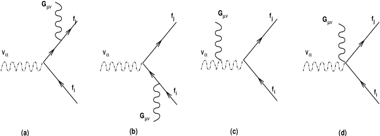
We see that the diagrams in figs. 1a-1c are obtained by attaching the spin-2 field in all possible ways to the external legs of the main diagram $V\to\bar{f}\,f$, while fig. 1d is given by the contact term $VVHG$.

Since we are interested in studying unpolarized processes, we recall here the formula for the sum over polarizations in the case of a massive spin-2 field. This is given by [18]

$$\sum_{\sigma=1}^{5}\epsilon_{\mu\nu}(k,\sigma)\,\epsilon_{\alpha\beta}(k,\sigma)=P_{\mu\nu\alpha\beta}(k)$$ (10)

$$P_{\mu\nu\alpha\beta}(k) = \frac{1}{2}\left(\eta_{\mu\alpha}\eta_{\nu\beta}+\eta_{\mu\beta}\eta_{\nu\alpha}-\eta_{\mu\nu}\eta_{\alpha\beta}\right)$$ (11)

$$- \frac{1}{2\,m_{G}^{2}}\left(\eta_{\mu\alpha}k_{\mu}k_{\beta}+\eta_{\nu\beta}k_{\mu}k_{\alpha}+\eta_{\mu\beta}k_{\nu}k_{\beta}+\eta_{\nu\alpha}k_{\mu}k_{\beta}\right)$$

$$+ \frac{1}{6}\left(\eta_{\mu\nu}+\frac{2}{m_{G}^{2}}k_{\mu}k_{\nu}\right)\left(\eta_{\alpha\beta}+\frac{2}{m_{G}^{2}}k_{\alpha}k_{\beta}\right),$$

where $\epsilon_{\mu\nu}(k,\sigma)$, $m_{G}$ and $k$ are the polarization tensor, mass and momentum of the spin-2 field, respectively, and the index $\sigma$ runs over the polarization states. Note that the projector $P_{\mu\nu\alpha\beta}$, which is symmetric and traceless in both $(\mu,\nu)$ and $(\alpha,\beta)$ indices, satisfies the transversality conditions $k^{\mu}P_{\mu\nu\alpha\beta}=k^{\alpha}P_{\mu\nu\alpha\beta}=0$. Then, by using the Lagrangian in eqs.(4) and (8), the square modulus of the amplitude ${\cal M}$ summed over all final polarizations and averaged over the initial ones, is

$$\frac{1}{3}\sum_{\rm pol}{|{\cal M}|^{2}}=N_{f}\frac{2\,g^{2}\,M_{V}^{2}}{3\,\bar{M}_{P}^{2}}\left(\left(|g_{V}|^{2}+|g_{A}|^{2}\right)\,F^{(+)}_{V}(t,u)+\left(|g_{V}|^{2}-|g_{A}|^{2}\right)\,F^{(-)}_{V}(t,u)\right)$$ (12)

where $g$ is the gauge coupling constant, and $g_{V,A}$ are the vectorial and axial couplings defined in eq.(5). For fermion $f$, $N_{f}$ represents the sum over quantum numbers, whose generators commute with the gauge group generator associated to the vector $V$, like, for instance, the fermion color number in the case of realistic $Z$ or $W$ decays. We assume the two fermion masses degenerate (i.e., $M_{f_{i}}=M_{f_{j}}=M_{f}$). Then, we define the Mandelstam variables $t$ and $u$ as

$$t=\frac{1}{M_{V}^{2}}\,(p_{1}+p_{G})^{2}-x_{f},~{}~{}~{}u=\frac{1}{M_{V}^{2}}\,(p_{2}+p_{G})^{2}-x_{f},~{}~{}~{}s=x_{G}-t-u$$ (13)

where $x_{f}=\frac{M_{f}^{2}}{M_{V}^{2}}$, $x_{G}=\frac{m_{G}^{2}}{M_{V}^{2}}$, and $M_{V}$, $m_{G}$, $M_{f}$ are the masses of the gauge boson, graviton, fermion, respectively. The analytical expressions for the functions $F^{(\pm)}_{V}(t,u)$ (also depending on the variables $x_{f}$ and $x_{G}$) can be found in the appendix A2.

It is worth noticing that, despite the presence of $1/m_{G}^{2}$ terms in the sum over polarizations for the massive spin-2 fields, in the final expression for $F^{(\pm)}_{V}(t,u)$ (and analogously for the other decay functions in the appendix A2) $m_{G}$ appears only with positive powers. The cancellation of $1/m_{G}^{2}$ terms in the total amplitude is indeed ensured by the conservation (at the zeroth order in $h_{\mu\nu}$) of the on-shell matrix elements of the energy momentum tensor in eq.(8). Therefore, the terms proportional to $k_{\mu}$ in eq.(11) do not contribute to the final amplitude. As a severe check of our results, we used the complete expression for $P_{\mu\nu\alpha\beta}$ in eq.(11) and explicitly verified this property.

Although the limit for $m_{G}\to 0$ is smooth, our results for the square amplitudes summed over polarizations is not supposed to coincide in this limit with the massless graviton contribution. This is due to the well-known van Dam-Veltman discontinuity [18]. Our results only hold for $m_{G}\neq 0$. Indeed, the emission of a massless graviton should be calculated by using the proper massless projector (see, e.g., [18]), that differs from the massive one. For the purpose of our analysis the effect of not taking into account this discontinuity is not relevant, since the square modulus of the amplitude for a single massless graviton contribution is suppressed by $1/\bar{M}_{P}^{2}$.

As said above, we are interested in analyzing inclusive processes, where one sums over all the kinematically allowed KK graviton states. The mass splitting $\Delta m_{G}$ between different excitations is given by

$$\Delta m_{G}\sim\frac{1}{R}=M_{D}\left(\frac{M_{D}}{\bar{M}_{P}}\right)^{2/\delta}$$ (15)

(e.g., in the case $\delta<4$, for $M_{D}\sim$1 TeV, $\Delta m_{G}$ is less than a few KeV’s). This allows one to approximate the KK modes as a continuous spectrum, with a number density of modes $(dN)$ between $m_{G}$ and $m_{G}+dm_{G}$ given by [2]

$$dN=S_{\delta-1}\frac{\bar{M}_{P}^{2}}{M_{D}^{2+\delta}}m_{G}^{\delta-1}dm_{G}.$$ (16)

Here, $S_{\delta-1}$ is the surface of a unit-radius sphere in $\delta$ dimensions. Then, the integration over the number of KK states cancels the factor $1/\bar{M}_{P}^{2}$ of the single graviton emission.

Finally, the result for the inclusive total width $\Gamma(V\to f\bar{f}+G_{X})$, where $G_{X}$ indicates any KK graviton excitation up to the $M_{V}$ scale, is given by

$$\Gamma(V\to f\bar{f}\,+\,G_{X}) = N_{f}\frac{M_{V}^{3}\,G_{V}\,S_{\delta-1}}{96\,\pi^{3}\,\sqrt{2}}\left(\frac{M_{V}}{M_{D}}\right)^{2+\delta}\left(\left(|g_{V}|^{2}+|g_{A}|^{2}\right)I^{(+)}_{V}(x_{\Delta},x_{f},\delta)\right.$$ (17)

$$+ \left.\left(|g_{V}|^{2}-|g_{A}|^{2}\right)I^{(-)}_{V}(x_{\Delta},x_{f},\delta)\right)$$

where

$$I_{V}^{(\pm)}(x_{\Delta},x_{f},\delta)=\int_{x_{\Delta}}^{(1-2\sqrt{x_{f}})^{2}}\,d\,x_{G}\,\,\left(x_{G}\right)^{\frac{\delta}{2}-1}\,\int_{x_{G}+2\sqrt{x_{f}x_{G}}}^{1-2\sqrt{x_{f}}}\,d\,t\int_{u_{-}}^{u_{+}}\,d\,u\,F_{V}^{(\pm)}(t,u)$$ (18)

and

$$u_{\pm} = \frac{\left(-2x_{f}+x_{G}-t\right)t+x_{G}+t\pm\Delta}{2\left(t+x_{f}\right)}$$

$$\Delta = \sqrt{\left(\left(x_{G}-t\right)^{2}-4x_{f}x_{G}\right)\left(1+t^{2}-2\left(2x_{f}+t\right)\right)},~{}~{}~{}x_{\Delta}=\frac{\Delta_{\rm exp}^{2}}{M_{V}^{2}}$$ (19)

We defined $G_{V}=g^{2}/(4\,\sqrt{2}\,M_{V}^{2})$ extending the definition of the standard Fermi constant $G_{F}$. $\Delta_{\rm exp}$ is the experimental resolution on the invariant mass of missing energy. Notice that the function $I_{V}^{(-)}(x_{\Delta},x_{f},\delta)$, that is proportional to the fermion masses, vanishes in the $x_{f}\to 0$ limit. The integral over the phase space is also regular in the $x_{\Delta}\to 0$ limit. This property is connected to the absence of graviton mass singularities in the square amplitude.

In table 1, we report some numerical values of the integrals $I_{V}^{(+)}(x_{\Delta},x_{f},\delta)$ in eq.(18), evaluated at $x_{\Delta}=0$ and $x_{f}=0$, for the representative cases $\delta=2,3,\dots,6$.

${\rm\delta}$	$I_{V}^{(+)}$	$I_{f}$	$I_{H}^{f}$	$I_{H}^{V}$
$2$	$1.20\times 10^{-1}$	$5.53\times 10^{-2}$	$3.25\times 10^{-1}$	$7.78\times 10^{-2}$
$3$	$2.12\times 10^{-2}$	$8.72\times 10^{-3}$	$4.95\times 10^{-2}$	$1.17\times 10^{-2}$
$4$	$5.85\times 10^{-3}$	$2.10\times 10^{-3}$	$1.14\times 10^{-2}$	$2.67\times 10^{-3}$
$5$	$2.11\times 10^{-3}$	$6.57\times 10^{-4}$	$3.35\times 10^{-3}$	$7.86\times 10^{-4}$
$6$	$9.13\times 10^{-4}$	$2.45\times 10^{-4}$	$1.18\times 10^{-3}$	$2.76\times 10^{-4}$

Table 1: Numerical values for $I^{(+)}_{V}(x_{\Delta},x_{f},\delta),~{}I_{f}(x_{\Delta},x_{V},\delta),~{}I_{H}^{f}(x_{\Delta},x_{f},\delta)$, and $I_{H}^{V}(x_{\Delta},x_{V},\delta)$ evaluated at $x_{\Delta}=x_{V}=x_{f}=0$, and for $\delta=2,3,4,5,6$.

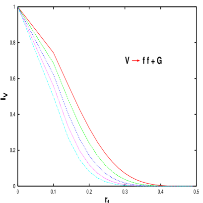
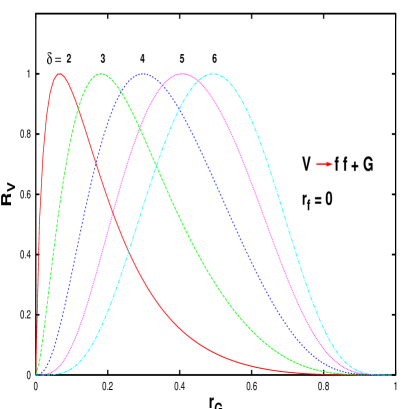
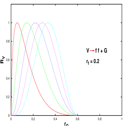
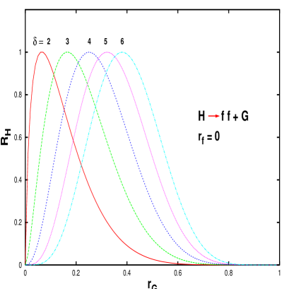
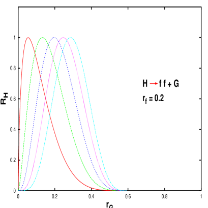
In fig. 2, we plot the integrals $I_{V}^{(+)}(x_{\Delta},x_{f},\delta)$ (evaluated at $x_{\Delta}=0$ and divided by their values at $x_{f}=0$ [see table 1]) versus $x_{f}$, and for $\delta=2,3,\dots,6$. In fig. 3, we plot the differential widths versus the ratio $r_{G}=m_{G}/M_{V}$, and for $\delta=2,3,\dots,6$. In particular, we plot the distribution $R$, normalized as

$$R=\frac{1}{\frac{d\Gamma}{dr_{G}}|_{{\rm max}}}~{}\frac{d\Gamma}{dr_{G}}$$ (20)

where $\frac{d\Gamma}{dr_{G}}|_{{\rm max}}$ stands for the maximum of $\frac{d\Gamma}{dr_{G}}$ versus $r_{G}$. The shape of this distribution provides information on the typical fraction of missing energy, due to the KK gravitons emission, expected in the decay. We analyze two representative cases: $M_{f}=0$ and $M_{f}=0.2~{}M_{V}$. From these results, we see that the position of the maximum ($r^{max}$) of the distributions $R$ is quite sensitive to the number of extra dimensions, going from $r^{\rm max}\simeq 0.1$, for $\delta=2$, up to $r^{\rm max}\simeq 0.5$, for $\delta=6$. When the mass for the final fermion is taken into account, these curves shift toward lower $r_{G}$ values, due to the phase-space reduction of the allowed $x_{G}$ range.

We recall that our perturbative treatment is bound to be valid for decaying particles not heavier than $M_{D}$. Indeed, being gravity directly coupled to the energy momentum tensor, the validity of the perturbative expansion strongly depends on the energy scale of the process with respect to the Planck mass $M_{D}$. Since in the relevant scenarios $M_{D}$ could be close to the TeV scale, this question is not just academic. In [2], when considering direct graviton production at colliders, upper bounds on the center of mass energy as a function of $M_{D}$ and number of extra dimensions have been obtained by requiring unitarity of the tree-level cross sections for single graviton production. In our case, if new particles exist with masses either larger than or close to the fundamental Planck scale $M_{D}$, then non-perturbative gravitational phenomena should sizeably affect their decay width. For instance, mass upper bounds that somewhat limit the perturbative regime can be obtained by requiring that the rate for one graviton emission from the main particle decay does not exceed the rate of its main decay. In particular, one can impose

$$\frac{\Gamma(V\to f\bar{f}+G_{X})}{\Gamma(V\to f\bar{f})}<1$$ (21)

for any fermion $f$ and for $\Delta_{\rm exp}=0$. In the approximation of massless fermions the width of $V\to f\bar{f}$ is given by

$$\Gamma(V\to f\bar{f})=N_{f}\frac{2\,M_{V}^{3}\,G_{V}}{3\,\pi\,\sqrt{2}}\left(|g_{V}|^{2}+|g_{A}|^{2}\right)$$ (22)

then from Eq.(21), one obtains

$$M_{V}<M_{D}\left(\frac{64\,\pi^{2}}{I^{(+)}_{V}(x_{\Delta},0,\delta)\,S_{\delta-1}}\right)^{\frac{1}{2+\delta}}\,.$$ (23)

From the values of the integrals given in table 1, for $x_{\Delta}=0$ we find

$$M_{V}<M_{D}\times\left(5.4,~{}4.7,~{}4.2,~{}3.8,~{}3.5\right),$$ (24)

for $\delta=2,3,4,5,6$, respectively. For massive fermions, the value of $I^{(+)}_{V}$ would be smaller (due to a smaller available phase space), giving less stringent upper bounds on $M_{V}$.

As a phenomenological application of this study, we analyze now the constraints on $M_{D}$ which come from negative searches of extra missing energy events in the $Z$ decays. In particular, we will consider the process

$$Z\to\,\bar{f}\,f\,+\,G_{X}$$ (25)

where $f$ may indicate leptons and quarks. The massless limit for the final fermion states is quite accurate in this case. From eq.(22), the decay width of $Z\to f_{i}\bar{f}_{i}$ for massless fermions is simply

$$\Gamma(Z\to f\bar{f})=N_{f}\frac{2\,M_{Z}^{3}\,G_{F}}{3\,\pi\,\sqrt{2}}\left(|g_{V}^{f}|^{2}+|g_{A}^{f}|^{2}\right)$$ (26)

where $N_{f}=1$ and 3 for leptons and quarks respectively, and $g^{f}_{A}=T^{f}_{3}/2$, $g^{f}_{V}=\left(T_{3}^{f}-2Q^{f}\sin{\theta_{W}}^{2}\right)/2$, being $T_{3}^{f}$ and $Q^{f}$ the eigenvalues of the third component of isotopic spin ($T_{3}^{e}=-\frac{1}{2}$) and electric charge, respectively. Here, the vectorial and axial couplings have been properly normalized after the introduction of the true Fermi constant $G_{F}$. Then, the branching ratio (BR) for the inclusive decay $Z\to\sum_{f}f\bar{f}+G_{X}$, where $f$ stands for any quark or lepton in the final state, is given by

$${\rm BR}(Z\to\sum_{f}f\bar{f}+G_{X})=\frac{S_{\delta-1}}{64\,\pi^{2}}\left(\frac{M_{Z}}{M_{D}}\right)^{2+\delta}\,I_{V}^{(+)}(x_{\Delta},0,\delta)$$ (27)

In the case $\delta=2$, and for $x_{\Delta}=x_{f}=0$, we obtain

$${\rm BR}(Z\to\sum_{f}f\bar{f}+G_{X})=\frac{8.2\times 10^{-8}}{M^{4}_{D}({\rm TeV})}$$ (28)

The result in eq.(28) agrees with the corresponding one in [17], after identifying $M^{4}_{\star}=2\,M_{D}^{4}$ for $\delta=2$, being the definition of $M_{\star}$ in [17] different from $M_{D}$ in eq.(1) ($G_{N}^{-1}=4\pi R^{\delta}M_{\star}^{2+\delta}$). Note that in [17] some graviscalar contribution is included.

These results can be extended to the decay $W^{\pm}\to ff^{\prime}+G$, in the massless limit for final fermions. In the latter case, the width and inclusive BR can be simply obtained from the $Z$ case, by replacing $M_{Z}\to M_{W}$ in eq.(27). In the case $\delta=2$, and for $x_{\Delta}=0$, we obtain

$${\rm BR}(W^{\pm}\to\sum_{f,f^{\prime}}f^{\prime}\bar{f}+G_{X})=\frac{5.0\times 10^{-8}}{M^{4}_{D}({\rm TeV})}$$ (29)

where $f\neq f^{\prime}$ run over the leptons and quarks with $T_{3}^{f}=1/2$ and $T_{3}^{f^{\prime}}=-1/2$.

The result in eq.(28) can be applied to the LEP1 data on $Z\to f\bar{f}+E_{miss}$, corresponding to about $2\times 10^{7}$ $Z$ decays. The SM background, given by the four-fermion decay $Z\to f\bar{f}\nu\bar{\nu}$, is very small. A few events that are quite in agreement with the SM prediction were observed [20]. Assuming, one can push the limit on unexpected signals down to BR($Z\to\sum_{f}f\bar{f}+G_{X})<10^{-7}$, one then gets, for $\delta=2$,

$$M_{D}>951\,{\rm GeV}$$ (30)

This limit is not far from what is obtained from the negative searches at LEP2 in the channel $e^{+}e^{-}\to\gamma\,+\,E_{miss}$, (where $E_{miss}$ is the missing energy due to gravitons emission) and from virtual gravitons effects [21].

4 Heavy Fermions and Top decays

We consider now a heavy fermion $f_{i}$ decaying into a lighter fermion $f_{j}$ plus a massive vector boson and a graviton

$$f_{i}(p_{i})\to f_{j}(p_{j})\,V(p_{V})+G(p_{G})$$ (31)

This class of processes includes the decay of the top quark $t\to Wb+G$ in the SM, that we will discuss later on. By summing over all final polarizations and averaging over initial ones, the square modulus of the amplitude for the process (31) is given, in the massless limit for $f_{j}$, by

$$\frac{1}{2}\sum_{\rm pol}{|{\cal M}|^{2}}=\frac{g^{2}\,M_{f}^{4}\,|K_{ij}|^{2}}{\bar{M}_{P}^{2}\,M_{V}^{2}}\left(|g_{V}|^{2}+|g_{A}|^{2}\right)\,F_{f}(t,u)$$ (32)

where the expression for the function $F_{f}(t,u)$ can be found in the appendix A2. Here, the Mandelstam variables are defined as

$$t=\frac{1}{M_{f_{i}}^{2}}\,(p_{i}-p_{G})^{2}-1\,,~{}~{}~{}u=\frac{1}{M_{f_{i}}^{2}}\,(p_{i}-p_{V})^{2}\,,~{}~{}~{}s=x_{G}-t-u\,,$$ (33)

where $p_{i}^{2}=M_{f_{i}}^{2},~{}~{}p_{V}^{2}=M_{V}^{2}$, $x_{V}\equiv\frac{M_{V}^{2}}{M_{f_{i}}^{2}}$ and $x_{G}\equiv\frac{m_{G}^{2}}{M_{f_{i}}^{2}}$. By the same procedure explained in the previous section, we got the total width $\Gamma(f_{i}\to f_{j}\,V\,+\,G_{X})$ for the inclusive KK graviton production. In the massless limit for $f_{j}$, this is given by

$$\Gamma(f_{i}\to f_{j}\,V\,+\,G_{X})=\frac{M_{f}^{3}\,G_{V}|K_{ij}|^{2}\,S_{\delta-1}}{64\,\pi^{3}\,\sqrt{2}}\left(|g_{V}|^{2}+|g_{A}|^{2}\right)\left(\frac{M_{f}}{M_{D}}\right)^{2+\delta}\,I_{f}(x_{\Delta},x_{f},\delta)$$ (34)

where $G_{V}=g^{2}/(4\,\sqrt{2}\,M_{V}^{2})$, and

$$I_{f}(x_{\Delta},x_{V},\delta)=\int_{x_{\Delta}}^{\left(1-\sqrt{x_{V}}\right)^{2}}\,d\,x_{G}\,\,\left(x_{G}\right)^{\delta/2-1}\,\int_{x_{G}}^{\left(1-\sqrt{x_{V}}\right)^{2}}\,d\,u\int_{t_{-}}^{t_{+}}\,d\,t\,F_{f}(t,u)$$

$$t_{\pm} = \frac{u-x_{G}}{2\,u}\left(1-u-x_{V}\right)\left(1\pm\Delta\right)-1+x_{V}\,~{}~{}~{}~{}\Delta=\sqrt{1-\frac{4ux_{V}}{(1-u-x_{V})^{2}}}\,$$ (35)

with $x_{\Delta}=\frac{\Delta_{\rm exp}^{2}}{M_{f_{i}}^{2}}$.

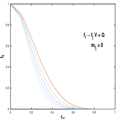
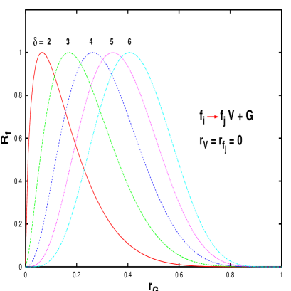
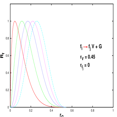
In table 1, we present the numerical results for $I_{f}(x_{\Delta},x_{V},\delta)$, at $x_{\Delta}=x_{V}=0$, and in fig. 2 we plot the function $I_{f}(0,x_{V},\delta)/I_{f}(0,0,\delta)$ versus $x_{V}$, for representative values $\delta=2,3,\dots,6$. In fig. 3, we plot the differential widths defined in eq.(20) versus $r_{G}\equiv\sqrt{x_{G}}$, and for $\delta=2,3,\dots,6$. We consider both the massless vector boson case and the massive case with $r_{V}=0.45$. This value of $r_{V}$ is relevant in the top quark decay, where $r_{W}=M_{W}/M_{t}\simeq 0.45$ ($M_{t}$ is the top quark mass). By comparing the distributions of the vector boson and fermion decays in fig. 3, we see that in general the positions of the maximum for the fermion distributions are closer to zero than in the vector boson case.

By requiring unitarity for the perturbative expansion,

$$\frac{\Gamma(f_{i}\to f_{j}\,V+G)}{\Gamma(f_{i}\to f_{j}\,V)}<1$$ (36)

where the total width $\Gamma(f_{i}\to f_{j}\,V)$ (in the $f_{j}$ massless limit) is

$$\Gamma(f_{i}\to f_{j}\,V\,)=\frac{M_{f_{i}}^{3}\,G_{V}|K_{ij}|^{2}}{2\,\pi\,\sqrt{2}}\left(|g_{V}|^{2}+|g_{A}|^{2}\right)\rho(x_{V})$$ (37)

and $\rho(x)=1-3x^{2}+2x^{3}$, we obtain

$$M_{f_{i}}<M_{D}\left(\frac{32\,\rho(x_{V})\,\pi^{2}}{I_{f}(x_{\Delta},x_{V},\delta)\,S_{\delta-1}}\right)^{\frac{1}{2+\delta}}\,.$$ (38)

From the $I_{f}$ values in table 1, we get for $x_{V}=x_{\Delta}=0$ the following limits from unitarity

$$M_{f}<M_{D}\times\left(5.5,~{}4.9,~{}4.4,~{}4.0,~{}3.8\right),$$ (39)

where the numbers inside parenthesis correspond to $\delta=2,3,4,5,6$, respectively.

Now we apply these results to the specific case of the top quark decays, where $V=W^{\pm}$ and $g_{V}=-g_{A}=\frac{1}{2\sqrt{2}}$. The top total width (at tree level, and neglecting CKM nondiagonal decays) is, in the $b$ massless limit

$$\Gamma(t\to W\,b)=\frac{M_{t}^{3}\,G_{F}|V_{tb}|^{2}}{8\,\pi\,\sqrt{2}}\rho(x_{W})$$ (40)

where $\rho(x_{W})=0.887$, and $V_{ij}$ is the standard CKM matrix. Then the total inclusive $BR$ for any $\delta$ is given by

$${\rm BR}(t\to W\,b\,+\,G_{X})=\frac{S_{\delta-1}}{32\,\pi^{2}}\left(\frac{M_{t}}{M_{D}}\right)^{2+\delta}\frac{I_{f}(x_{\Delta},x_{W},\delta)}{\rho(x_{W})}$$ (41)

In the case $\delta=2$, and $x_{\Delta}=0$, we obtain

$${\rm BR}(t\to Wb+G_{X})=\frac{1.8\times 10^{-7}}{M^{4}_{D}({\rm TeV})}$$ (42)

being $I_{f}(0,x_{W},2)=8.38\times 10^{-3}$ (for $M_{t}=175$GeV).

It can be interesting to compare this value, with the rates expected for other rare top quark decays both inside and beyond the standard model, also considering the potential of future accelerators in this field [22]. In case of negative searches for this signal, one will impose an experimental upper bound on the BR of this decay: ${\rm BR}(t\to W\,b\,+\,G_{X})<\Delta_{exp}^{\rm top}$, where $\Delta_{exp}^{\rm top}$ is related to the experimental sensitivity on the top branching ratio. Then, one finds, for $\delta=2$,

$$M_{D}>\left(\Delta_{exp}^{\rm top}\right)^{-\frac{1}{4}}\,0.22\,M_{Z}$$ (43)

where we expressed the mass scale $M_{t}$ on the right hand side through $M_{Z}$. Then, we can compare this result with the corresponding one for the Z decay, obtained from eq.(27) for $\delta=2$,

$$M_{D}>\left(\Delta_{exp}^{Z}\right)^{-\frac{1}{4}}\,0.19\,M_{Z}$$ (44)

where ${\rm BR}(Z\to\bar{f}f\,+\,G_{X})<\Delta_{exp}^{Z}$ is assumed. We see that, assuming (at present, quite unrealistically) a comparable sensitivity on the two BR’s, the lower bounds on $M_{D}$ obtained from the gravitational $Z$ and top decays turn out to be comparable, too.

5 Higgs boson decays

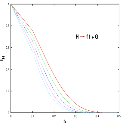
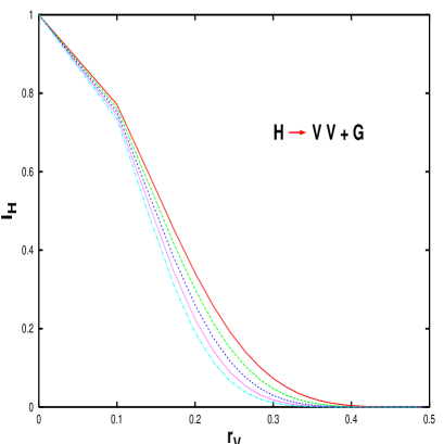
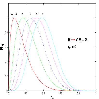
In this section, we analyze the gravitational emission in the Higgs boson decays into either two massive gauge bosons or two fermions,

$$H(p_{H}) \to V(p_{1})\,\,V(p_{2})\,+\,G(p_{G})$$

$$H(p_{H}) \to \bar{f}(p_{1})\,f(p_{2})+G(p_{G}).$$ (45)

Using the interaction vertices given in section 2, we obtain the following expressions for the square modulus of the amplitudes summed over polarizations

$$\sum_{\rm pol}{|{\cal M}_{H\to V\,V\,+\,G}|^{2}} = \frac{g^{2}\,M_{H}^{4}}{6\,\bar{M}_{P}^{2}\,M_{V}^{2}}\,F_{H}^{V}(t,u)$$

$$\sum_{\rm pol}{|{\cal M}_{H\to\bar{f}\,f\,+\,G}|^{2}} = N_{f}\frac{\lambda_{f}^{2}\,M_{H}^{2}}{3\,\bar{M}_{P}^{2}}\,F_{H}^{f}(t,u)$$ (46)

where the functions $F_{\rm H}^{V,f}(t,u)$ can be found in appendix A2. The definition of Mandelstam variables $t,u$, and $s$ is given by

$$t=\frac{1}{M_{H}^{2}}\,(p_{1}+p_{G})^{2}\,-\,x_{f,V},~{}~{}~{}u=\frac{1}{M_{H}^{2}}\,(p_{2}+p_{G})^{2}\,-\,x_{f,V},~{}~{}~{}s=x_{G}-t-u$$ (47)

with $x_{i}=\frac{M_{i}^{2}}{M_{H}^{2}}$, $i=V,F$. Then, the inclusive total widths are given by

$$\Gamma(H\to V\,V\,+\,G_{X}) = \kappa\frac{M_{H}^{3}\,G_{V}\,S_{\delta-1}}{384\,\pi^{3}\,\sqrt{2}}\left(\frac{M_{H}}{M_{D}}\right)^{2+\delta}I_{\rm H}^{V}(x_{\Delta},x_{V},\delta)$$ (48)

$$\Gamma(H\to\bar{f}\,f+G_{X}) = N_{f}\frac{M_{H}\,\lambda_{f}^{2}\,S_{\delta-1}}{1536\,\pi^{3}}\left(\frac{M_{H}}{M_{D}}\right)^{2+\delta}I^{f}_{\rm H}(x_{\Delta},x_{f},\delta)$$ (49)

where

$$I_{\rm H}^{V,f}(x_{\Delta},x_{(f,V)},\delta)=\int d\,x_{G}\,\,\left(x_{G}\right)^{\delta/2-1}\,\int\,d\,t\int\,d\,u\,F^{V,f}_{\rm H}(t,u).$$ (50)

Here, the integration limits are the same as in $V\to\bar{f}f+G$ (see eq.(18)), with $x_{f}\to x_{V}$ in the case of $I_{H}^{V}$. The coefficient $\kappa$ in eq.(48) is equal to 1, unless the two final vector bosons are identical particles. In the latter case, $\kappa=\frac{1}{2}$.

The tree level decay widths of $H\to\bar{f}f$ and $H\to VV$ are given by

$$\Gamma(H\to\bar{f}\,f)=N_{f}\frac{M_{H}\,\lambda_{f}^{2}}{8\,\pi}\rho_{f}(x_{f}),~{}~{}~{}~{}\Gamma(H\to V\,V)=\kappa\frac{M_{H}^{3}\,G_{V}}{8\,\pi\,\sqrt{2}}\rho_{V}(x_{V})$$ (51)

where $\rho_{f}=\left(1-4x\right)^{\frac{3}{2}}$ and $\rho_{V}(x)=\sqrt{1-4x}~{}(1-4x+12x^{2})$.

The unitarity conditions here require

$$M_{H}<M_{D}\left(\frac{192\,\rho_{f}(x_{f})\,\pi^{2}}{I_{H}^{f}(x_{\Delta},x_{f},\delta)\,S_{\delta-1}}\right)^{\frac{1}{2+\delta}}\,,~{}~{}~{}~{}~{}M_{H}<M_{D}\left(\frac{48\,\rho_{V}(x_{V})\,\pi^{2}}{I_{H}^{V}(x_{\Delta},x_{V},\delta)\,S_{\delta-1}}\right)^{\frac{1}{2+\delta}}\,$$ (52)

for $H\to\bar{f}f+G$ and $H\to VV+G$, respectively. In the limit $x_{f}^{2},~{}x_{V}^{2}\to 0$ and $x_{\Delta}=0$, we get

$$M_{H}<M_{D}\times\left(5.5,~{}5.0,~{}4.5,~{}4.2,~{}3.9\right),~{}~{}~{}M_{H}<M_{D}\times\left(5.6,~{}5.0,~{}4.6,~{}4.2,~{}3.9\right),$$ (53)

for $\delta=2,3,4,5,6$, respectively.

As an application of our results, we can consider two representative scenarios in the SM: the light ($M_{H}<2M_{W}$) and the heavy ($M_{H}>2M_{t}$) Higgs boson. In particular, we set $M_{H}=120$ GeV and $M_{H}=500$ GeV, respectively. Then, approximating the total $H$ width by the dominant tree-level $\Gamma(b\bar{b})$ and $\Gamma(t\bar{t}+WW+ZZ)$, respectively, the gravitational decays BR’s are given by

• Light Higgs ($M_{H}<2M_{W}$)

  $${\rm BR}(H\to\bar{b}b+G)=\left(\frac{S_{\delta-1}}{192\pi^{2}\rho_{f}(x_{b})}\right)\left(\frac{M_{H}}{M_{D}}\right)^{2+\delta}I_{H}^{F}(x_{\Delta},x_{b},\delta)$$ (54)

• Heavy Higgs ($M_{H}>2M_{t}$)

  $${\rm BR}(H\to WW+G) = \left(\frac{S_{\delta-1}}{24\pi^{2}\Delta_{H}}\right)\left(\frac{M_{H}}{M_{D}}\right)^{2+\delta}\,I_{H}^{V}(x_{\Delta},x_{W},\delta)$$ (55)

  $${\rm BR}(H\to ZZ+G) = \left(\frac{S_{\delta-1}}{48\pi^{2}\Delta_{H}}\right)\left(\frac{M_{H}}{M_{D}}\right)^{2+\delta}\,I_{H}^{V}(x_{\Delta},x_{Z},\delta)$$ (56)

  $${\rm BR}(H\to\bar{t}t+G) = \left(\frac{S_{\delta-1}x_{t}}{16\pi^{2}\Delta_{H}}\right)\left(\frac{M_{H}}{M_{D}}\right)^{2+\delta}\,I_{H}^{f}(x_{\Delta},x_{t},\delta)$$ (57)

where the variables $x_{i}$ are defined as $x_{i}=M_{i}^{2}/M_{H}^{2}$, with $i=b,t,W,Z$, and $\Delta_{H}=12x_{t}\rho_{f}(x_{t})+2\rho_{V}(x_{W})+\rho_{V}(x_{Z})$. Note that, in eqs.(48) and (51), $G_{V}\to G_{F}$ for the $H$ decaying both into $W$’s and into $Z$’s.

In the case $\delta=2$, we obtain

$${\rm BR}(H\to\bar{b}b+G_{X}) = \frac{2.2\times 10^{-7}}{M^{4}_{D}({\rm TeV})},~{}~{}~{}~{}M_{H}=120~{}{\rm GeV}$$ (58)

$${\rm BR}(H\to W~{}W+G_{X}) = \frac{2.1\times 10^{-5}}{M^{4}_{D}({\rm TeV})},~{}~{}~{}~{}M_{H}=500~{}{\rm GeV}$$ (59)

$${\rm BR}(H\to Z~{}Z+G_{X}) = \frac{8.7\times 10^{-6}}{M^{4}_{D}({\rm TeV})},~{}~{}~{}~{}M_{H}=500~{}{\rm GeV}$$ (60)

$${\rm BR}(H\to\bar{t}~{}t+G_{X}) = \frac{8.7\times 10^{-7}}{M^{4}_{D}({\rm TeV})},~{}~{}~{}~{}M_{H}=500~{}{\rm GeV}$$ (61)

where we used, for $M_{H}=120$ GeV, $I_{H}^{f}(0,x_{b},2)=0.312$, and, for $M_{H}=500$ GeV, $I_{H}^{V}(0,x_{W},2)=0.0393$, $I_{H}^{V}(0,x_{Z},2)=0.0321$, and $I_{H}^{f}(0,x_{t},2)=0.00876$.

We can see that, in order to constrain $M_{D}$ in the range of a few TeV’s for $\delta=2$, we need a sensitivity on the Higgs BR’s of order ${\cal O}(10^{-7})$ and ${\cal O}(10^{-5})$, for the light and heavy Higgs boson, respectively. Higher sensitivities are needed to explore the case of a larger $\delta$. Such sensitivities on the Higgs BR’s are beyond the reach of any presently planned experiment by a few orders of magnitude. Anyhow, they could become of some interest for physics that might be studied at a Higgs boson factory in a not-near future (see, e.g.,[23]).

6 Conclusions

In this paper, we studied the effects of quantum gravity propagating in large extra dimensions in a few favoured decay channels of heavy particles. In particular, we analyzed the inclusive radiative emission of Kaluza-Klein spin-2 gravitons in the following decay channels: the two-fermions decays of massive gauge bosons, heavy quarks, Higgs bosons, and the two-massive gauge bosons decay of Higgs bosons.

Due to the huge number of KK gravitons radiated, the inclusive widths, for a particle of mass $M$, is only suppressed by a factor of order $\left(\frac{M}{M_{D}}\right)^{2+\delta}$, versus the usual factor $\left(\frac{M}{M_{P}}\right)^{2}$ arising in quantum gravity in 3+1 dimensions. If the mass of the particle is pretty close to the Plank mass in D-dimensions $M_{D}$, the quantum gravity effects might sizeably affect the heavy particles decays. In scenarios where the SM fields propagate in extra dimensions with a $\sim$ TeV compactification scale, good candidates for the decaying heavy particles might be the KK excitations of the usual SM particles.

In this framework, we provided analytical results for the square modulus of the amplitudes, and numerical results for the inclusive widths. Final-state masses have been taken into account, apart from the case of a heavy fermion decay, where a massless final fermion is assumed. Since, experimentally, the KK gravitons are indirectly detected by measuring missing energy and mass in the decay process, we presented plots for the distributions of the widths versus the KK graviton mass. We showed that the position of the maximum for each distribution is quite sensitive to the number of extra dimensions.

We also discussed the validity of the present perturbative approach for heavier masses of the decaying particles. We showed that, when the mass of the decaying particles is a few times $M_{D}$, the radiative widths exceed the corresponding tree-level widths, breaking unitarity. While there are not unitarity problems in the effective theory for $M<M_{D}$, one should keep in mind that, for larger masses, non perturbative effects get in general important.

As an application of our study, we analyzed the decays $Z\to\bar{f}f+G$,   $W\to\bar{f}^{\prime}f+G$,   $t\to Wb+G$,   $H\to\bar{f}f+G$, and $H\to WW+G$, that can be of interest at present and future experiments. In the case of $Z$ decays, the present sensitivity on the BR($Z\to\bar{f}f+E_{miss})$ at LEP1 can push the lower bound on $M_{D}$ from this decay channel not far from the bounds obtained at LEP2 [21]. Similar bounds are obtained from the top quark gravitational decay, assuming (quite unrealistically, at present) that some day the experimental sensitivity on its BR will get close to the $Z$ one at LEP1. For the Higgs boson decay, we considered the two representative cases of a light ($m_{H}=120$ GeV) and heavy ($m_{H}=500$ GeV) Higgs. We showed that, in order to set lower bounds on $M_{D}$ of order a few TeV’s for $\delta=2$, a sensitivity $\sim 10^{-7}$ and $\sim 10^{-5}$, respectively, on its gravitational BR’s is required. The latter sensitivities are definitely a few orders of magnitude beyond the reach of the planned experiments for Higgs production and study.

Appendix A1

In this appendix we report the Feynman rules for gravitational interactions which are relevant for the processes considered in this article. In particular, by means of eqs.(4) and (8), we obtain

where we used the convention that particle momenta (indicated inside parenthesis) flow along the arrow directions. The expressions of $W$ and $X$ quantities, corresponding to 3-line and 4-line interaction vertices, respectively, involving 2-vectors ($W^{(V)},~{}X^{(V)}$), 2-fermions ($W^{(f)},~{}X^{(f)}$), and 2-Higgs bosons ($W^{(H)}$), are given below.

• Vector

  $$W^{(V)}_{\mu\nu\alpha\beta} = -\frac{i}{\bar{M}_{P}}\left\{\frac{1}{2}\eta_{\mu\nu}\left(k_{2\alpha}k_{1\beta}-\eta_{\alpha\beta}\,k_{1}\cdot k_{2}\right)+\eta_{\alpha\beta}k_{1\mu}k_{2\nu}-\eta_{\mu\beta}k_{1\nu}k_{2\alpha}\right.$$ (62)

  $$+ \left.\eta_{\mu\alpha}\left(\eta_{\nu\beta}\,k_{1}\cdot k_{2}-k_{2\nu}k_{1\beta}\right)+M_{V}^{2}\left(\eta_{\mu\alpha}\eta_{\nu\beta}-\frac{1}{2}\eta_{\mu\nu}\eta_{\alpha\beta}\right)\right\}$$

  $$X^{(V)}_{\mu\nu\alpha\beta} = -\frac{i}{\bar{M}_{P}}g\,M_{V}\left(\eta_{\mu\alpha}\eta_{\nu\beta}-\frac{1}{2}\eta_{\mu\nu}\eta_{\alpha\beta}\right)$$ (63)

• Fermion

  $$W^{(f)}_{\mu\nu} = -\frac{i}{4\bar{M}_{P}}\left\{\gamma_{\mu}\left(k_{1\nu}+k_{2\nu}\right)-\eta_{\mu\nu}\left(\hat{k}_{1}+\hat{k}_{2}-M_{f_{i}}\right)\right\}$$ (64)

  $$X^{(f)}_{\mu\nu\alpha} = -\frac{i}{2\bar{M}_{P}}g\left(\gamma_{\mu}\eta_{\nu\alpha}-\gamma_{\alpha}\eta_{\mu\nu}\right)\left(g_{V}+g_{A}\gamma_{5}\right)$$ (65)

  $$X^{(f)} = -\frac{i}{\bar{M}_{P}}\lambda_{f_{i}}$$ (66)

• Higgs boson

  $$W^{(H)}_{\mu\nu} = -\frac{i}{\bar{M}_{P}}\left\{k_{1\mu}k_{2\nu}-\frac{1}{4}\eta_{\mu\nu}\left(k_{1}\cdot k_{2}-M_{H}^{2}\right)\right\}$$ (67)

where the symbol $\hat{p}$ stands for $\hat{p}\equiv\gamma^{\alpha}p_{\alpha}$.

Appendix A2

In this appendix we report the expressions for the functions $F_{V}^{(\pm)}(t,u)$, $F_{f}(t,u)$, and $F_{H}^{V,f}(t,u)$ appearing in eqs.(12), (32), and (46) respectively. Everywhere, the relation $s=x_{G}-t-u$ holds.

$\bullet$    ${\bf V\to\bar{f}\,\,f\,+\,G}$

$$F_{\rm V}^{(\pm)}(t,u) = \sum_{i=1}^{10}\,T^{(\pm)}_{i}$$

$$T_{1}^{(+)} = -\frac{1}{3\,s^{2}}\left\{-16+22\,t-6\,{t^{2}}+22\,u-2\,t\,u-6\,{u^{2}}+16\,x_{f}-32\,t\,x_{f}\right.$$

$$+ \left.{t^{2}}\,x_{f}-32\,u\,x_{f}+2\,t\,u\,x_{f}+{u^{2}}\,x_{f}+2\,{x_{G}^{2}}\,\left(-7+2\,x_{f}\right)\right.$$

$$- \left.2\,x_{G}\,\left(22-7\,t-7\,u-32\,x_{f}+2\,t\,x_{f}+2\,u\,x_{f}\right)\right\}$$

$$T_{1}^{(-)} = -\frac{x_{f}}{3\,s^{2}}\left\{48-56\,t+13\,{t^{2}}-56\,u+26\,t\,u+13\,{u^{2}}\right.$$

$$- \left.4\,\left(-28+13\,t+13\,u\right)\,x_{G}+52\,{x_{G}^{2}}\right\}$$

$$T_{2}^{(+)} = \frac{1}{6\,t^{2}}\left(-1+x_{f}\right)\left(3\,{x_{G}^{2}}-4\,x_{G}\,x_{f}-32\,{x_{f}^{2}}\right)$$

$$T^{(-)}_{2} = \frac{x_{f}}{2\,t^{2}}\left(3\,{x_{G}^{2}}-4\,x_{G}\,x_{f}-32\,{x_{f}^{2}}\right)$$

$$T_{3}^{(\pm)} = \left\{T_{2}^{(\pm)}~{}~{}(u\leftrightarrow t)\right\}$$

$$T_{4}^{(+)} = \frac{1}{6\,ts}\left\{24+36\,u+12\,{u^{2}}+{x_{G}^{3}}\,\left(6-12\,x_{f}\right)-56\,x_{f}-68\,u\,x_{f}\right.$$

$$- \left.14\,{u^{2}}\,x_{f}+3\,{u^{3}}\,x_{f}+32\,{x_{f}^{2}}+56\,u\,{x_{f}^{2}}-4\,{u^{2}}\,{x_{f}^{2}}\right.$$

$$- \left.2\,{x_{G}^{2}}\,\left(3+6\,u+2\,x_{f}-12\,u\,x_{f}+8\,{x_{f}^{2}}\right)\right.$$

$$+ \left.x_{G}\,\left(-12-6\,u+6\,{u^{2}}+48\,x_{f}+18\,u\,x_{f}-15\,{u^{2}}\,x_{f}\right.\right.$$

$$- \left.\left.-112\,{x_{f}^{2}}+16\,u\,{x_{f}^{2}}\right)\right\}$$

$$T_{4}^{(-)} = -\frac{x_{f}}{6\,ts}\left\{12\,{x_{G}^{3}}+4\,{x_{G}^{2}}\,\left(-9-6\,u+4\,x_{f}\right)\right.$$

$$+ \left.x_{G}\,\left(-32+6\,u+15\,{u^{2}}+16\,x_{f}-16\,u\,x_{f}\right)\right.$$

$$+ \left.\left(u-6\right)\,\left(-12-12\,u-3\,{u^{2}}+16\,x_{f}+4\,u\,x_{f}\right)\right\}$$

$$T_{5}^{(\pm)} = \left\{T_{4}^{(\pm)}~{}~{}(u\leftrightarrow t)\right\}$$

$$T_{6}^{(+)} = \frac{1}{3\,tu}\left\{12+3\,{x_{G}^{3}}-18\,{x_{G}^{2}}\,\left(-1+x_{f}\right)-60\,x_{f}+80\,{x_{f}^{2}}-32\,{x_{f}^{3}}\right.$$

$$+ \left.x_{G}\,\left(27-75\,x_{f}+32\,{x_{f}^{2}}\right)\right\}$$

$$T_{6}^{(-)} = -\frac{x_{f}}{3\,tu}\left\{36+39\,x_{G}+8\,{x_{G}^{2}}-144\,x_{f}-56\,x_{G}\,x_{f}+96\,{x_{f}^{2}}\right\}$$

$$T_{7}^{(+)} = \frac{1}{6\,s}\left\{56\,{x_{G}^{2}}\,x_{f}+x_{G}\,\left(88-28\,x_{f}-53\,t\,x_{f}-53\,u\,x_{f}+32\,{x_{f}^{2}}\right)\right.$$

$$- \left.2\,\left(-42+10\,t-3\,{t^{2}}+10\,u+6\,t\,u-3\,{u^{2}}+64\,x_{f}+11\,t\,x_{f}\right.\right.$$

$$- \left.\left.7\,{t^{2}}\,x_{f}+11\,u\,x_{f}-11\,t\,u\,x_{f}-7\,{u^{2}}\,x_{f}-56\,{x_{f}^{2}}+6\,t\,{x_{f}^{2}}+6\,u\,{x_{f}^{2}}\right)\right\}$$

$$T_{7}^{(-)} = \frac{x_{f}}{6\,s}\left\{56\,{x_{G}^{2}}+x_{G}\,\left(20-53\,t-53\,u+32\,x_{f}\right)\right.$$

$$- \left.2\,\left(88+47\,t-7\,{t^{2}}+47\,u-11\,t\,u-7\,{u^{2}}-8\,x_{f}+6\,t\,x_{f}+6\,u\,x_{f}\right)\right\}$$

$$T_{8}^{(+)} = \frac{1}{6\,u}\left\{36+12\,t+12\,{x_{G}^{2}}\,\left(-1+x_{f}\right)-12\,x_{f}-24\,t\,x_{f}\right.$$

$$+ \left.3\,{t^{2}}\,x_{f}-14\,t\,{x_{f}^{2}}+x_{G}\,\left(9\,t+30\,x_{f}-9\,t\,x_{f}+16\,{x_{f}^{2}}\right)\right\}$$

$$T_{8}^{(-)} = \frac{x_{f}}{6\,u}\left\{-60-6\,t+3\,{t^{2}}+12\,{x_{G}^{2}}-160\,x_{f}-14\,t\,x_{f}\right.$$

$$+ \left.x_{G}\,\left(-18-9\,t+16\,x_{f}\right)\right\}$$

$$T_{9}^{(\pm)} = \left\{T_{8}^{(\pm)}~{}~{}(u\leftrightarrow t)\right\}$$

$$T_{10}^{(+)} = -\frac{1}{6}\left\{8+6\,t+6\,u+22\,x_{f}+t\,x_{f}+u\,x_{f}+28\,{x_{f}^{2}}+12\,x_{G}\,\left(-1+2\,x_{f}\right)\right\}$$

$$T_{10}^{(-)} = -\frac{x_{f}}{6}\left(130+t+u+24\,x_{G}+28\,x_{f}\right)$$

$\bullet$    ${\bf f_{i}\to f_{j}\,\,V\,+\,G}$

$$F_{\rm f}(t,u) = \sum_{i=1}^{10}\,F_{i}$$

$$F_{1} = \frac{1}{6\,s^{2}}\left\{{{\left(t+u-2\,x_{G}\right)}^{2}}+x_{V}\,\left(-12\,t+11\,{t^{2}}-9\,{u^{2}}+24\,x_{G}-24\,t\,x_{G}\right.\right.$$

$$+ \left.\left.4\,{x_{G}^{2}}+2\,u\,\left(-6+t+8\,x_{G}\right)\right)-4\,\,{x_{V}^{2}}\,\left(-4+8\,t+3\,{t^{2}}+3\,{u^{2}}\right.\right.$$

$$+ \left.\left.u\,\left(8+t-7\,x_{G}\right)-16\,x_{G}-7\,t\,x_{G}+7\,{x_{G}^{2}}\right)\right.$$

$$+ \left.4\,{x_{V}^{3}}\,\left(4+11\,t+11\,u-22\,x_{G}\right)-32\,{x_{V}^{4}}\right\}$$

$$F_{2} = \frac{1}{12\,t^{2}}\left(-32-4\,x_{G}+3\,{x_{G}^{2}}\right)\,\left(-1-x_{V}+2\,{x_{V}^{2}}\right)$$

$$F_{3} = \frac{{x_{G}^{2}}}{4\,u^{2}}\,\left(-1-x_{V}+2\,{x_{V}^{2}}\right)$$

$$F_{4} = \frac{1}{6\,ts}\left\{12-3\,{u^{3}}-4\,x_{G}-2\,{x_{G}^{2}}+6\,{x_{G}^{3}}+4\,{u^{2}}\,\left(-1+3\,x_{G}\right)\right.$$

$$+ \left.u\,\left(2+6\,x_{G}-15\,{x_{G}^{2}}\right)-2\,x_{V}\,\left(-10-32\,x_{G}-8\,{x_{G}^{2}}+3\,{x_{G}^{3}}\right.\right.$$

$$+ \left.\left.{u^{2}}\,\left(-4+3\,x_{G}\right)+u\,\left(14+12\,x_{G}-6\,{x_{G}^{2}}\right)\right)\right.$$

$$- \left.2\,{x_{V}^{2}}\,\left(2+6\,{u^{2}}+12\,x_{G}-3\,{x_{G}^{2}}-u\,\left(7+3\,x_{G}\right)\right)\right.$$

$$- \left.4\,{x_{V}^{3}}\,\left(1+9\,u-3\,x_{G}\right)-24\,{x_{V}^{4}}\right\}$$

$$F_{5} = \frac{1}{us}\left\{2+6\,x_{G}+5\,{x_{G}^{2}}+{x_{G}^{3}}+\frac{t^{2}}{2}\,\left(2+x_{G}\right)-\frac{t}{2}\,\left(6+10\,x_{G}+3\,{x_{G}^{2}}\right)\right.$$

$$- \left.\,x_{V}\,\left(2+{t^{2}}\,\left(-1+x_{G}\right)+4\,x_{G}+2\,{x_{G}^{2}}+{x_{G}^{3}}-t\,x_{G}\,\left(1+2\,x_{G}\right)\right)\right.$$

$$+ \left.{x_{V}^{2}}\,\left(-6-2\,{t^{2}}-4\,x_{G}+{x_{G}^{2}}+t\,\left(9+x_{G}\right)\right)+2\,{x_{V}^{3}}\,\left(5-3\,t+x_{G}\right)-4\,{x_{V}^{4}}\right\}$$

$$F_{6} = \frac{1}{2\,tu}\left\{4+x_{G}-{x_{G}^{2}}-2\,x_{V}\,\left(2+4\,x_{G}-3\,{x_{G}^{2}}+{x_{G}^{3}}\right)\right.$$

$$+ \left.{x_{V}^{2}}\,\left(-12+25\,x_{G}-12\,{x_{G}^{2}}\right)+{x_{V}^{3}}\,\left(20-18\,x_{G}\right)-8\,{x_{V}^{4}}\right\}$$

$$F_{7} = \frac{1}{6\,s}\left\{-10\,{u^{2}}+u\,\left(34-11\,t+31\,x_{G}\right)\right.$$

$$- \left.2\,\left(8-22\,t+2\,{t^{2}}+36\,x_{G}-11\,t\,x_{G}+14\,{x_{G}^{2}}\right)\right.$$

$$- \left.2\,x_{V}\,\left(6-5\,t+3\,{t^{2}}-6\,\left(1+t\right)\,u+3\,{u^{2}}-7\,x_{G}\right)\right.$$

$$+ \left.4\,{x_{V}^{2}}\,\left(16+5\,t+5\,u-22\,x_{G}\right)-84\,{x_{V}^{3}}\right\}$$

$$F_{8} = \frac{1}{u}\left\{-3+t-\frac{9}{2}\,x_{G}+\frac{t}{4}\,x_{G}-{x_{G}^{2}}+x_{V}\,\left(t-\frac{3}{2}\,t\,x_{G}+\frac{x_{G}}{2}\,\left(3+4\,x_{G}\right)\right)\right.$$

$$+ \left.{x_{V}^{2}}\,\left(9-2\,t\right)-6\,{x_{V}^{3}}\right\}$$

$$F_{9} = \frac{1}{t}\left\{\frac{1}{12}\left(-6\,{u^{2}}+u\,\left(2+15\,x_{G}\right)+6\,\left(10+x_{G}-2\,{x_{G}^{2}}\right)\right)\right.$$

$$- \left.\frac{x_{V}}{2}\left(3\,u\,\left(-2+x_{G}\right)+\left(13-4\,x_{G}\right)\,x_{G}\right)-{x_{V}^{2}}\,\left(7+2\,u\right)-6\,{x_{V}^{3}}\right\}$$

$$F_{10} = \frac{1}{6}\left\{55+2\,t-u+12\,x_{G}+x_{V}\,\left(11+6\,t+6\,u-12\,x_{G}\right)+8\,{x_{V}^{2}}\right\}$$ (69)

$\bullet$    ${\bf H\to V\,\,V\,+\,G}$

$$F_{\rm H}^{V}(t,u) = \sum_{i=1}^{10}\,H^{V}_{i}$$

$$H^{V}_{1} = \frac{1}{4\,s^{2}}\left\{\left(16+{t^{2}}+20\,u+{u^{2}}+2\,t\,\left(10+u\right)-4\,\left(7+t+u\right)\,x_{G}+4\,{x_{G}^{2}}\right)\right.$$

$$\times \left.\left(1-4\,x_{V}+12\,{x_{V}^{2}}\right)\right\}$$

$$H^{V}_{2} = \frac{1}{t^{2}}\left\{{x_{G}^{2}}\,\left({\frac{1}{4}}-6\,x_{V}+13\,{x_{V}^{2}}\right)+{x_{V}^{2}}\,\left(4-5\,{u^{2}}-16\,x_{V}+48\,{x_{V}^{2}}\right)\right.$$

$$+ \left.x_{G}\,x_{V}\,\left(3+5\,u-12\,x_{V}+56\,{x_{V}^{2}}\right)\right\}$$

$$H^{V}_{3} = \left\{H^{V}_{2}~{}~{}(u\leftrightarrow t)\right\}$$

$$H^{V}_{4} = \frac{1}{ts}\left\{3-16\,x_{V}-{u^{3}}\,x_{V}+52\,{x_{V}^{2}}-48\,{x_{V}^{3}}+{x_{G}^{3}}\,\left(-1+6\,x_{V}\right)\right.$$

$$+ \left.{u^{2}}\,\left(3-11\,x_{V}+14\,{x_{V}^{2}}\right)+\frac{3\,x_{G}^{2}}{2}\,\left(4+u-24\,x_{V}-6\,u\,x_{V}+32\,{x_{V}^{2}}\right)\right.$$

$$+ \left.u\,\left(6-23\,x_{V}+48\,{x_{V}^{2}}-12\,{x_{V}^{3}}\right)+x_{G}\,\left({u^{2}}\,\left(-{\frac{1}{2}}+5\,x_{V}\right)\right.\right.$$

$$+ \left.\left.u\,\left(-{\frac{17}{2}}+41\,x_{V}-52\,{x_{V}^{2}}\right)+4\,\left(-2+11\,x_{V}-23\,{x_{V}^{2}}+6\,{x_{V}^{3}}\right)\right)\right\}$$

$$H^{V}_{5} = \left\{H^{V}_{4}~{}~{}(u\leftrightarrow t)\right\}$$

$$H^{V}_{6} = \frac{1}{tu}\left\{3-24\,x_{V}+92\,{x_{V}^{2}}-176\,{x_{V}^{3}}+96\,{x_{V}^{4}}+{x_{G}^{2}}\,\left({\frac{1}{2}}+2\,x_{V}+26\,{x_{V}^{2}}\right)\right.$$

$$+ \left.x_{G}\,\left(3-4\,x_{V}-44\,{x_{V}^{2}}+112\,{x_{V}^{3}}\right)\right\}$$

$$H^{V}_{7} = \frac{1}{s}\left\{24+19\,u+{u^{2}}+{x_{G}^{2}}\,\left(5-22\,x_{V}\right)+{t^{2}}\,\left(1-4\,x_{V}\right)\right.$$

$$- \left.94\,x_{V}-69\,u\,x_{V}-4\,{u^{2}}\,x_{V}+240\,{x_{V}^{2}}+114\,u\,{x_{V}^{2}}-24\,{x_{V}^{3}}\right.$$

$$+ \left.t\,\left(19+2\,u-69\,x_{V}-6\,u\,x_{V}+114\,{x_{V}^{2}}\right)\right.$$

$$+ \left.\frac{x_{G}}{2}\,\left(-60-9\,u+252\,x_{V}+34\,u\,x_{V}-424\,{x_{V}^{2}}+t\,\left(-9+34\,x_{V}\right)\right)\right\}$$

$$H^{V}_{8} = \frac{1}{u}\left\{6+{x_{G}^{2}}\,\left(1-6\,x_{V}\right)-16\,x_{V}-7\,{t^{2}}\,x_{V}+20\,{x_{V}^{2}}+72\,{x_{V}^{3}}\right.$$

$$+ \left.t\,\left(3-6\,x_{V}+4\,{x_{V}^{2}}\right)+x_{G}\,\left(-8+29\,x_{V}+8\,{x_{V}^{2}}+t\,\left(-{\frac{1}{2}}+10\,x_{V}\right)\right)\right\}$$

$$H^{V}_{9} = \left\{H^{V}_{8}~{}~{}(u\leftrightarrow t)\right\}$$

$$H^{V}_{10} = 19+t+u-70\,x_{V}-9\,t\,x_{V}-9\,u\,x_{V}+126\,{x_{V}^{2}}+x_{G}\,\left(-3+22\,x_{V}\right)$$

$\bullet$    ${\bf H\to\bar{f}\,\,f\,+\,G}$

$$F_{\rm H}^{f}(t,u) = \sum_{i=1}^{10}\,H^{f}_{i}$$

$$H^{f}_{1} = \frac{1}{s^{2}}\left(4+t+u-2\,x_{G}\right)^{2}$$

$$H^{f}_{2} = \frac{1}{t^{2}}\left\{{\frac{-3\,{x_{G}^{2}}}{2}}+2\,x_{G}\,x_{f}+16\,{x_{f}^{2}}\right\}$$

$$H^{f}_{3} = \left\{H^{f}_{2}~{}~{}(u\leftrightarrow t)\right\}$$

$$H^{f}_{4} = \frac{1}{ts}\left\{-2\,\left(-2-u+2\,x_{G}\right)\,\left(3\,\left(1+u\right)-\left(4+u\right)\,x_{f}+x_{G}\,\left(-3+2\,x_{f}\right)\right)\right\}$$

$$H^{f}_{5} = \left\{H^{f}_{4}~{}~{}(u\leftrightarrow t)\right\}$$

$$H^{f}_{6} = \frac{1}{tu}\left\{12+x_{G}\,\left(9-8\,x_{f}\right)-48\,x_{f}+32\,{x_{f}^{2}}\right\}$$

$$H^{f}_{7} = \frac{1}{s}\left\{72+28\,t+{t^{2}}+28\,u+2\,t\,u+{u^{2}}+4\,{x_{G}^{2}}-6\,\left(4+t+u\right)\,x_{f}\right.$$

$$+ \left.4\,x_{G}\,\left(-14-t-u+4\,x_{f}\right)\right\}$$

$$H^{f}_{8} = \frac{1}{u}\left\{6\,\left(3+t\right)+\left(16-7\,t\right)\,x_{f}+x_{G}\,\left(-15+{\frac{3\,t}{2}}+8\,x_{f}\right)\right\}$$

$$H^{f}_{9} = \left\{H^{f}_{8}~{}~{}(u\leftrightarrow t)\right\}$$

$$H^{f}_{10} = 39-5\,t-5\,u-14\,x_{f}$$

Figure 2: Values of the integrals $I_{V}$ (top-left) , $I_{\rm F}$ (top-right), $I_{H}^{f}$ (bottom-left), and $I_{H}^{V}$ (bottom-right) versus $r_{V}$, $r_{f_{j}}$, $r_{f}$, and $r_{V}$ respectively, evaluated at $x_{\Delta}=0$, and divided by their corresponding values at $x_{i}=0$. A superscript $I^{(+)}$ is understood for $I_{V}$. In each plot, lower curves correspond to higher extra dimensions, for $\delta=2,3,4,5,6$, respectively. Here, $r_{i}=\frac{M_{i}}{M}$, $x_{i}=r_{i}^{2}$, where $M$ is the mass of the decaying particle.

Figure 3: Widths distributions $R=\frac{1}{\frac{d\Gamma}{dr_{G}}|_{{\rm max}}}~{}\frac{d\Gamma}{dr_{G}}$, versus $r_{G}$, for $x_{\Delta}=0$, and for $\delta=2,3,4,5,6$. Here, $r_{G}=\frac{m_{G}}{M}$, $r_{i}=\frac{M_{i}}{M}$ with $i=f,V$ and $M$ is the mass of the decaying particle. Plots relative to the $V\to\bar{f}f+G$ and $f_{i}\to f_{j}V+G$ decays are shown.

Figure 4: Width distributions as in figure (3), but for the processes $H\to\bar{f}f+G$, and $H\to VV+G$.

References

- [1] N. Arkani-Hamed, S. Dimopoulos, and G. Dvali, Phys. Lett. B429 (1998) 263.
- [2] G. F. Giudice, R. Rattazzi, and J. D. Wells, Nucl. Phys. B 544 (1999) 3.
- [3] T. Han, J. D. Lykken, and R. Zhang, Phys. Rev. D 59 (1999) 105006.
- [4] E. A. Mirabelli, M. Perelstein, and M. E. Perskin, Phys. Rev. Lett. 82 (1999) 2236; J. L. Hewett, Phys. Rev. Lett. 82 (1999) 4765; E. Dudas and J. Mourad, Nucl. Phys. B 575 (2000) 3; E. Accomando, I. Antoniadis, and K. Benakli, Nucl. Phys. B 579 (2000) 3; S. Cullen, M. Perelstein, and M. E. Peskin, Phys. Rev. D 62 (2000) 055012; W. D. Goldberger and M. B. Wise, Phys. Lett. B475 (2000) 275; B. Grzadkowski and J.F. Gunion, Phys. Lett. B473 (2000) 50; G. F. Giudice, R. Rattazzi, and J. D. Wells, hep-ph/0112161.
- [5] G. F. Giudice, R. Rattazzi, and J. D. Wells, Nucl. Phys. B 595 (2001) 250.
- [6] For a realization of the Higgs graviscalar mixing in string theory see, I. Antoniadis, R. Sturani, hep-ph/0201166.
- [7] I. Antoniadis, N. Arkani-Hamed, S. Dimopoulos, and G. Dvali, Phys. Lett. B436 (1998) 257; G. Shiu and S. H. Tye, Phys. Rev. D58 (1998) 106007; G. Shiu, R. Shrock, and S. H. Tye, Phys. Lett. B458 (1999) 274; Z. Kakushadze and S. H. Tye, Nucl. Phys. B548 (1999) 180; I. Antoniadis, C. Bachas, and E. Dudas, Nucl. Phys. B560 (1999) 93; G. Aldazabal, L. E. Ibanez and F. Quevedo, JHEP 0001 (2000) 031.
- [8] S. Dimopoulos and G. F. Giudice, Phys. Lett. B379 (1996) 105 J.C. Long, H. W. Chan and J. C. Price, Nucl.Phys.B539:23-34,1999.
- [9] L. Randall and R. Sundrum, Phys. Rev. Lett. 83 (1999) 3370; Phys. Rev. Lett. 83 (1999) 4690.
- [10] H. Davoudiasl, J. L. Hewett, and T. G. Rizzo Phys. Rev. Lett. 84 (2000) 2080; Phys. Lett. B473 (2000) 43; Phys. Rev. D63 (2001) 075004.
- [11] A. De Rujula, A. Donini, M.B. Gavela, and S. Rigolin, Phys. Lett. B482 (2000) 195.
- [12] T. G. Rizzo, Phys. Rev. D64 (2001) 095010.
- [13] I. Antoniadis, Phys. Lett B246 (1990) 377; I. Antoniadis, C. Muñoz, and M. Quiros, Nucl. Phys. B397 (1993) 515; I. Antoniadis and K. Benakli, Phys. Lett. B326 (1994) 69; I. Antoniadis, K. Benakli, and M. Quiros, Phys. Lett. B331 (1994) 313; K. Benakli Phys. Lett. B386 (1996) 106; T. Appelquist, H.-C. Cheng, and B. A. Dobrescu, Phys. Rev. D64 (2001) 035002; R. Barbieri, L.J. Hall, and Y. Nomura, Phys. Rev. D63 (2001) 105007;
- [14] K. R. Dienes, E. Dudas, T. Gherghetta, Nucl. Phys. B537 (1999) 47.
- [15] K. R. Dienes, E. Dudas, T. Gherghetta, Nucl. Phys. B557 (1999) 25.
- [16] P. Nath and M. Yamaguchi, Phys. Rev. D60 (1999) 116006; M. Masip and A. Pomarol, Phys. Rev. D60 (1999) 096005; W. J. Marciano, Phys. Rev. D60 (1999) 093006; L. Hall and C. Kolda, Phys. Lett. B459 (1999) 213; R. Casalbuoni, S. DeCurtis, and D. Dominici, Phys. Lett. B462 (1999) 48; A. Strumia, Phys. Lett. B466 (1999) 107; F. Cornet, M. Relano, and J. Rico, Phys. Rev. D61 (2000) 037701; C. D. Carone, Phys. Rev. D61 (2000) 015008; A. Delgado, A. Pomarol, and M. Quiros, JHEP 0001 (2000) 030; T. G. Rizzo and J. D. Wells, Phys. Rev. D61 (2000) 016007.
- [17] C. Balázs, H.-J. He, W. W. Repko, C.-P. Yuan, Phys. Rev. Lett. 83 (1999) 2112.
- [18] H. van Dam and M. Veltman, Nucl. Phys. B22 (1970) 397.
- [19] J.A.M. Vermaseren, Symbolic Manipulation with FORM, published by CAN (Computer Algebra Nederland), Kruislaan 413, 1098 SJ Amsterdam, 1991, ISBN 90-74116-01-9.
- [20] M. Kobel, arXiv:hep-ex/9611015, and references therein.
- [21] G. Landsberg, arXiv:hep-ex/0105039, and references therein.
- [22] M. Beneke et al., Proc. of the Workshop on Standard Model Physics (and more) at the LHC, G.Altarelli and M.L.Mangano editors, report CERN 2000-004, p. 419-529, arXiv:hep-ph/0003033.
-
[23]
“Higgs Factory 2001 Snowmass Report”,
http://www.physics.ucla.edu/hep/hfactory/index.html