Phenomenological Constraints on Extended Quark Sectors

Abstract

We study the flavor physics in two extensions of the quark sector of the Standard Model (SM): a four generation model and a model with a single vector–like down–type quark (VDQ). In our analysis we take into account the experimental constraints from tree–level charged current processes, rare Kaon decay processes, rare $B$ decay processes, the $Z\to b\bar{b}$ decay, $K$, $B$ and $D$ mass differences, and the CP violating parameters $\frac{\varepsilon^{\prime}}{\varepsilon}$, $\varepsilon_{K}$ and $a_{\psi K}$. All the constraints are taken at two sigma. We find bounds on parameters which can be used to represent the New Physics contributions in these models ($\lambda_{t^{\prime}}^{bd}$, $\lambda_{t^{\prime}}^{bs}$ and $\lambda_{t^{\prime}}^{sd}$ in the four–generation model, and $U_{bd}$, $U_{bs}$ and $U_{sd}$ in the VDQ model) due to all the above constraints. In both models the predicted ranges for $a_{SL}$ (the CP asymmetry in semi-leptonic decays), $\Delta M_{D}$, $B(K^{+}\to\pi^{+}\nu\bar{\nu})$, $B(K_{L}\to\pi^{0}\nu\bar{\nu})$ and $B(K_{L}\to\mu\bar{\mu})_{SD}$ can be significantly higher than the predictions of the SM, while the allowed ranges for $a_{\psi K}$ and for $\Delta m_{B_{S}}$ are consistent with the SM prediction.

1 Introduction

Extensions of the quark sector modify many features of the Standard Model flavor physics. In particular, CKM unitarity is violated, and there are new sources of flavor–changing neutral–currents (FCNC) and of CP violation. We here analyze the flavor physics of two such extensions: a fourth generation of fermions and a single vector–like representation of quarks added to the SM.

These two models share many common aspects. Both models have the same number of mixing angles and phases, which can be taken as parameters of a $4\times 4$ unitary matrix. Both models violate the $3\times 3$ CKM unitarity in a similar manner, and introduce new sources of CP violation. Although originating from different Feynmann diagrams, many of the expressions for the experimental observables in the two models are practically the same (except for numerical differences). The features of CKM non-unitarity and new CP violating parameters are of particular interest, since they offer us a behavior which is qualitatively different from that of the SM. Also, the two models provide new contributions to FCNC processes. Since FCNC are highly suppressed in the SM, they provide a useful tool in searching for New Physics and in constraining it.

In order to constrain the models, we consider the new contributions to rare $K$ and $B$ decays, neutral meson mixing mass differences, CP violating parameters in the $K$ and in the $B$ systems, and the process $Z\to b\bar{b}$. To obtain the numerical results, we scan the allowed ranges of the mixing parameters. For each point in this parameter space, we check that all the above mentioned constraints are obeyed. This gives us bounds on the possible values of the mixing parameters and the correlations between them. We also use the scan to give predictions for various observables in these models, and compare them to the predictions in the SM. Finally, we analyze the predictions of these models to various processes that are not measured yet, such as $K^{+}\to\pi^{+}\nu\bar{\nu}$, $K_{L}\to\pi^{0}\nu\bar{\nu}$, $B\to X_{s}\ell^{+}\ell^{-}$, $\Delta M_{D}$ and $\Delta M_{B_{S}}$.

The paper is organized as follows. In section 2 we describe the analysis for the four generation model, and in section 3 we describe the analysis for the VDQ model. Each of these sections includes some background about the model, descriptions of the various constraints used in the analysis, and the details of the numerical results. Finally, in section 4 we discuss our conclusions.

2 A four generation model

2.1 Background

Currently there is no known fundamental principle which fixes the number of SM generations. Regarding experimental constraints, as of today there is no conclusive evidence that excludes a fourth generation. There are, however, two problematic issues. First, the invisible decay width of the $Z^{0}$ boson clearly indicates the existence of exactly three light neutrinos. The existence of a fourth neutrino with mass $m_{\nu 4}\geq 45$ GeV is not excluded by the data, but it requires some mechanism that will give the new neutrino a large mass while keeping the masses of the SM neutrinos small. Second, the four–generation model has some difficulties in explaining the electroweak precision measurements. Various analyzes of electroweak precision measurements (e.g. [1] and [2]) differ in their conclusions regarding the implications for a fourth generation. We assume that these measurements are consistent with four generations. Specifically, our analysis can be viewed as complementary to the one in ref. [2], taking into account also the mixing in the quark sector.

The constraints we consider are the following: charged–current tree–level decays, the branching ratios $B(K^{+}\to\pi^{+}\nu\bar{\nu})$, $B(K_{L}\to\mu\bar{\mu})_{SD}$ and $B(B\to X_{s}\ell^{+}\ell^{-})$, the mass differences $\Delta m_{K}$, $\Delta m_{B_{d}}$, $\Delta m_{B_{s}}$ and $\Delta m_{D}$, the CP violating parameters $\varepsilon_{K}$ and $a_{\psi K}$, and the partial decay width of $Z\to b\bar{b}$.

An extensive work on this subject can be found in [3]. We add to it the $B\to\psi K_{S}$ constraint, which was not available at the time, and the $Z\to b\bar{b}$ constraint. Also, we treat $B(B\to X_{s}\ell^{+}\ell^{-})$ in a more careful manner. In addition, we update the experimental bounds used in [3] and we consider the entire range of possible mixing angles and phases. Another work which considered the tree–level decays, a rough analysis of the $Z\to b\bar{b}$ process and the $B$ meson system constraints, can be found in [4].

2.2 The model

We consider a model with an extra generation of chiral fermions added to the SM in the simplest possible way. The representations of the fourth generation fermions are identical to the representations of the usual three SM generations. In such a model, there are nine additional parameters compared to the SM: four new masses, and five new mixing angles and phases. The origin of the new mixing angles and phases comes from the fact that the CKM matrix is now a $4\times 4$ matrix. This means that it consists of nine physical parameters: six mixing angles (compared to three in the SM) and three complex phases (compared to one in the SM). We use a specific parametrization of the $4\times 4$ CKM matrix [5], in order to incorporate all the correlations in the analysis which we perform. The mixing angles will be referred to as $\theta_{12},\theta_{13},\theta_{23},\theta_{14},\theta_{24}$ and $\theta_{34}$, and the phases as $\phi_{13},\phi_{14}$ and $\phi_{24}$. In the limit of vanishing new mixing angles, one gets the usual mixing angles $\theta_{12},\theta_{13},\theta_{23}$ and the CP violating phase $\phi_{13}$ of the SM.

We deal only with the quark sector of the model, which includes the SM quarks as well as the new quarks (to be referred to as ($t^{\prime}\,\,b^{\prime}$)). The new leptons do not play any role in our analysis, and we do not discuss them. In particular, we do not restrict ourselves to any specific mechanism that gives rise to the high mass required for the fourth neutrino.

The effects of the fourth generation enter the processes we consider through loop diagrams: the new quarks $t^{\prime}$ and $b^{\prime}$ can now appear in the loops. In most of the constraints, the fourth generation contribution enters almost exclusively through the parameters $\lambda_{t^{\prime}}^{bd}$, $\lambda_{t^{\prime}}^{bs}$ and $\lambda_{t^{\prime}}^{sd}$, where

$$\lambda_{k}^{lm}\equiv V_{kl}^{*}V_{km}.$$ (1)

These parameters can be used to evaluate the effects of New Physics contributions.

2.3 The Constraints

The analyzes done in [1, 2] concerning electroweak precision measurements with four generations indicate that only a restricted range of $m_{t^{\prime}}-m_{b^{\prime}}$ is allowed:

$$|m_{t^{\prime}}-m_{b^{\prime}}|\leq 85\ \rm{GeV\ \ \ \ (at\ 95\%\ CL)}.$$ (2)

Another constraint on the masses comes from the combined results of direct measurements at CDF and D0 collaborations [6], which rule out $m_{b^{\prime}}\leq 175$ GeV, assuming that the FCNC decay mode is dominant. We assume hereafter $m_{t^{\prime}}\geq m_{b^{\prime}}\gtrsim 175$ GeV. Also, since a perturbative approach is assumed to be valid, one must require $m_{t^{\prime}}\,,\,m_{b^{\prime}}\lesssim 500$ GeV. In view of the above constraints, we consider in our analysis two extreme cases of the new fermion masses. The first uses the highest possible mass values (in view of the above constraints): $m_{t^{\prime}}=500$ GeV, $m_{b^{\prime}}=470$ GeV. The second uses $m_{t^{\prime}}=200$ GeV, $m_{b^{\prime}}=170$ GeV. For each of the two cases ($m_{t^{\prime}}=500$ GeV or $m_{t^{\prime}}=200$ GeV), any alternative choice for $m_{b^{\prime}}$ (which obeys the limitation given in eq. (2)) can cause only minor changes to the results we present in this work. The actual calculations for both cases ($m_{t^{\prime}}=500$ GeV and $m_{t^{\prime}}=200$ GeV) are basically the same, with only numerical differences. In order not to repeat the presentation twice, we give a detailed analysis only for the case $m_{t^{\prime}}=500$ GeV. The results for the second case (with $m_{t^{\prime}}=200$ GeV) are briefly summarized in section 2.7.

Measured SM tree–level processes are not affected by the existence of a fourth generation, and can therefore be used as in the SM to constrain elements of the CKM matrix. This enables us to bound the magnitude of the matrix elements $V_{ud},V_{us},V_{ub},V_{cd},V_{cs}$ and $V_{cb}$.

Parameter	Mean value	Sigma	Ref.
$\left|V_{ud}\right|$	$0.9735$	$0.0008$	[1]
$\left|V_{us}\right|$	$0.2205$	$0.0018$	[7]
$\left|V_{ub}\right|$	$0.00349$	$0.00076$	[7]
$\left|V_{cd}\right|$	$0.224$	$0.016$	[1]
$\left|V_{cs}\right|$	$0.996$	$0.024$	[8]
$\left|V_{cb}\right|$	$0.041$	$0.002$	[7]
$R_{b}$	$0.21653$	$0.00069$	[9]
$Br(K_{L}\to\mu\bar{\mu})_{SD}$	$\leq 3.75\times 10^{-9}$	95$\%$ CL	[10, 11]
$Br(K^{+}\to\pi^{+}\nu\bar{\nu})$	$\leq 5.07\times 10^{-10}$	95$\%$ CL	[12]
$Br(K_{L}\to\pi^{0}\nu\bar{\nu})$	$\leq 5.9\times 10^{-7}$	95$\%$ CL	[7]
$B(B\to X_{s}e^{+}e^{-})$	$\leq 1\times 10^{-5}$	90$\%$ CL	[13]
$\varepsilon_{K}$	$2.28\times 10^{-3}$	$0.013\times 10^{-3}$	[7]
${\varepsilon^{\prime}}\over\varepsilon$	$17.2\times 10^{-4}$	$1.8\times 10^{-4}$	[14]
$\Delta m_{K}$	$3.489\times 10^{-15}$ GeV	$0.008\times 10^{-15}$ GeV	[7]
$\Delta m_{B_{d}}$	$3.2\times 10^{-13}$ GeV	$0.092\times 10^{-13}$ GeV	[7]
$\Delta m_{B_{s}}$	$>9.87\times 10^{-12}$ GeV	95$\%$ CL	[7]
$a_{\psi K}$	0.8	0.1	[15, 16, 17]
$|M_{12}^{D}|$	$\leq 6.3\times 10^{-14}$ GeV	95$\%$ CL	[18]

Table 1: Values of experimental-related input parameters used in the analysis.

The parametrization of $V_{CKM}$ means that we can translate these constraints into bounds on some of the mixing angles. Taking the constraints as described in Table 1 at two sigma, and using unitarity of the $4\times 4\,V_{CKM}$ matrix, we deduce the following ranges:

$$\sin\theta_{12}=0.22\ ,$$

$$\sin\theta_{23}=0.041\pm 0.004\ ,$$

$$\sin\theta_{13}=0.00349\pm 0.00152\ ,$$

$$0\leq\sin\theta_{14}\lesssim 0.085\ ,$$

$$0\leq\sin\theta_{24}\lesssim 0.25\ .$$

These bounds are independent of the new quark masses. The parameter $\sin\theta_{34}$ and the CP violating phases $\phi_{13},\phi_{14}$ and $\phi_{24}$ remain unconstrained at this stage.

We now consider loop processes. These depend on the Inami-Lim functions [19] $X_{0}(x)$, $Y_{0}(x)$ and $S_{0}(x)$ defined in [20]. Experimental inputs are given in table 1 and theoretical ones in table 2. Most of the expressions for the various constraints in the four generation model are obtained in a simple manner from the relevant expressions for the SM, by considering additional diagrams with $t^{\prime}$ quarks in the loop.

Parameter	Value	Ref.
$f_{B_{d}}\sqrt{B_{B_{d}}}$	$0.23\pm 0.04$ GeV	[7]
$f_{D}\sqrt{B_{D}}$	$\geq 0.2$ GeV	[21]
$\xi=\frac{f_{B_{s}}\sqrt{B_{B_{s}}}}{f_{B_{d}}\sqrt{B_{B_{d}}}}$	$1.15\pm 0.06$	[7]
$f_{K}$	0.16 GeV	[7]
$B_{K}$	$0.85\pm 0.15$	[7]

Table 2: Values of decay constants and bag parameters used in the analysis.

The rare Kaon decays which we consider are $K_{L}\to\mu\bar{\mu}$ and $K^{+}\to\pi^{+}\nu\bar{\nu}$. A bound on $B(K_{L}\to\mu\bar{\mu})_{SD}$ (the short–distance contribution to the dispersive part of $B(K_{L}\to\mu\bar{\mu})$) can be extracted from the experimental data as described e.g. in ref. [7]. The expression for this quantity in the four generation model is given by

$$B(K_{L}\to\mu\bar{\mu})_{SD}=6.32\times 10^{-3}\times{\left[Y_{NL}Re\lambda_{c}^{sd}+{\eta_{t}}^{Y}Y_{0}(x_{t})Re\lambda_{t}^{sd}+{\eta_{t^{\prime}}}^{Y}Y_{0}(x_{t^{\prime}})Re\lambda_{t^{\prime}}^{sd}\right]}^{2},$$ (4)

where $Y_{NL}=(3.5\pm 0.6)\times 10^{-4}$ [20] represents the charm contribution. In our analysis we neglect the QCD correction factors ${\eta_{t}}^{Y}$ and ${\eta_{t^{\prime}}}^{Y}$, since they are close to unity. The expression for $B(K^{+}\to\pi^{+}\nu\bar{\nu})$ in the four generation model is given by

$$B(K^{+}\to\pi^{+}\nu\bar{\nu})=1.55\times 10^{-4}\times\left|\lambda_{t}^{sd}\eta_{t}^{X}X_{0}(x_{t})+\lambda_{t^{\prime}}^{sd}\eta_{t^{\prime}}^{X}X(x_{t^{\prime}})+X_{NL}\lambda_{c}^{sd}\right|^{2},$$ (5)

where $X_{NL}=(9.8\pm 1.4)\times 10^{-4}$ represents the charm contribution. In this case we again neglect the QCD corrections which are close to unity. We also neglect the uncertainty in $X_{NL}$.

Next we discuss mass differences in the various neutral meson systems. The four generation expression for the short–distance contribution to $\Delta m_{K}$ is given by

$$\Delta m_{K}^{SD}=\frac{G_{F}^{2}m_{W}^{2}f_{K}^{2}B_{K}m_{K}}{6\pi^{2}}Re[{\lambda_{c}^{sd}}^{2}\eta_{c}^{K}S_{0}(x_{c})+{\lambda_{t}^{sd}}^{2}\eta_{t}^{K}S_{0}(x_{t})+{\lambda_{t^{\prime}}^{sd}}^{2}\eta_{t^{\prime}}^{K}S_{0}(x_{t^{\prime}})+{}$$ (6)

$${}+2\lambda_{c}^{sd}\lambda_{t}^{sd}\eta_{ct}^{K}S_{0}(x_{c},x_{t})+2{\lambda_{c}^{sd}}{\lambda_{t^{\prime}}^{sd}}\eta_{ct^{\prime}}^{K}S_{0}(x_{c},x_{t^{\prime}})+2{\lambda_{t}^{sd}}{\lambda_{t^{\prime}}^{sd}}\eta_{tt^{\prime}}^{K}S_{0}(x_{t},x_{t^{\prime}})].$$

Assuming that the long–distance contributions can be at most of the order of the experimental value $\Delta m_{K}^{exp}$, we take this constraint as $0\lesssim\Delta m_{K}^{SD}\lesssim 7\times 10^{-15}$ GeV.

The contributions to the short–distance part of the $D^{0}-\bar{D^{0}}$ meson mixing amplitude $M_{12}$ in the SM are very small compared to the current experimental bound (by several orders of magnitude). The leading diagram for $M_{12}^{SD}$ in the four generation case contains two $b^{\prime}$ quarks in the loop, and is given by

$$|\ M_{12}^{SD}\ |=\frac{G_{F}^{2}m_{W}^{2}f_{D}^{2}B_{D}m_{D}}{12\pi^{2}}{|{V_{cb^{\prime}}^{*}}{V_{ub^{\prime}}^{*}}|}^{2}\eta_{b^{\prime}}S_{0}(x_{b^{\prime}})\ .$$ (7)

Since the long–distance contributions to $M_{12}$ are also estimated to be small compared to the experimental bound, we demand in the four–generation case $\left|M_{12}^{SD}\right|\leq 6.3\times 10^{-14}$ GeV, where the experimental bound was taken as in table 1 with $\eta_{b^{\prime}}=0.56$. The experimental bound we use is weaker than the one usually considered (e.g. in [1]) since it does not assume $\delta=0$ and uses instead the available experimental data [18]. From the parametrization of $V_{CKM}$, ${|V_{ub^{\prime}}V_{cb^{\prime}}|}^{2}\approx\sin^{2}\theta_{14}\sin^{2}\theta_{24}$, so eq. (7) gives the bound

$$\sin\theta_{14}\sin\theta_{24}\lesssim\left\{\begin{array}[]{l}4.1\times 10^{-3}\ \ \ \ m_{t^{\prime}}=500\ {\rm GeV}\\ 9.1\times 10^{-3}\ \ \ \ m_{t^{\prime}}=200\ {\rm GeV}\end{array}\right.$$ (8)

The four generation expression for $\Delta m_{B_{d}}$ is given by

$$\Delta m_{B_{d}}=\frac{G_{F}^{2}m_{W}^{2}f_{B_{d}}^{2}B_{B_{d}}m_{B_{d}}}{6\pi^{2}}\left|{\lambda_{t}^{bd}}^{2}\eta_{t}^{B}S_{0}(x_{t})+{\lambda_{t^{\prime}}^{bd}}^{2}\eta_{t^{\prime}}^{B}S_{0}(x_{t^{\prime}})+2{\lambda_{t}^{bd}}{\lambda_{t^{\prime}}^{bd}}\eta_{tt^{\prime}}^{B}S_{0}(x_{t},x_{t^{\prime}})\right|\ .$$ (9)

We take the QCD factors as $\eta_{t}^{B}=0.55$, $\eta_{tt^{\prime}}^{B}=0.5$ and $\eta_{t^{\prime}}^{B}=0.54$.

The expression for $\Delta m_{B_{s}}$ is the same as that for $\Delta m_{B_{d}}$, the only change is to replace $d\to s$ in all places. Using the input of tables 1 and 2, one obtains

$$\left|\frac{{\lambda_{t}^{bs}}^{2}\eta_{t}^{B}S_{0}(x_{t})+{\lambda_{t^{\prime}}^{bs}}^{2}\eta_{t^{\prime}}^{B}S_{0}(x_{t^{\prime}})+2{\lambda_{t}^{bs}}{\lambda_{t^{\prime}}^{bs}}\eta_{tt^{\prime}}^{B}S_{0}(x_{t},x_{t^{\prime}})}{{\lambda_{t}^{bd}}^{2}\eta_{t}^{B}S_{0}(x_{t})+{\lambda_{t^{\prime}}^{bd}}^{2}\eta_{t^{\prime}}^{B}S_{0}(x_{t^{\prime}})+2{\lambda_{t}^{bd}}{\lambda_{t^{\prime}}^{bd}}\eta_{tt^{\prime}}^{B}S_{0}(x_{t},x_{t^{\prime}})}\right|\gtrsim 19.6\ .$$ (10)

Next we consider the $\varepsilon_{K}$ constraint. In a four generation model, one has

$$\varepsilon_{K}=\frac{1}{2}C_{\varepsilon}B_{K}\times Im[{\lambda_{c}^{sd}}^{*^{2}}\eta_{c}^{K}S_{0}(x_{c})+{\lambda_{t}^{sd}}^{*^{2}}\eta_{t}^{K}S_{0}(x_{t})+{\lambda_{t^{\prime}}^{sd}}^{*^{2}}\eta_{t^{\prime}}^{K}S_{0}(x_{t^{\prime}})\ +$$ (11)

$${}+2{\lambda_{c}^{sd}}^{*}{\lambda_{t}^{sd}}^{*}\eta_{ct}^{K}S_{0}(x_{c},x_{t})+2{\lambda_{c}^{sd}}^{*}{\lambda_{t^{\prime}}^{sd}}^{*}\eta_{ct^{\prime}}^{K}S_{0}(x_{c},x_{t^{\prime}})+2{\lambda_{t}^{sd}}^{*}{\lambda_{t^{\prime}}^{sd}}^{*}\eta_{tt^{\prime}}^{K}S_{0}(x_{t},x_{t^{\prime}})]\ .$$

where $C_{\varepsilon}\equiv G_{F}^{2}m_{W}^{2}f_{K}^{2}m_{K}/(6\pi^{2}\sqrt{2}\Delta m_{K})=3.8\times 10^{4}$. For the SM QCD corrections we take [7] $\eta_{t}^{K}=0.57$, $\eta_{c}^{K}=1.38$ and $\eta_{ct}^{K}=0.47$. For the new QCD corrections we take [3] $\eta^{K}_{t^{\prime}t^{\prime}}=0.57$, $\eta^{K}_{tt^{\prime}}=0.6$ and $\eta^{K}_{ct^{\prime}}=0.5$.

Another constraint, $a_{\psi K}$, comes from the decays $B\to\psi K$. In the SM, this quantity measures to an excellent approximation $\sin 2\beta$, where $\beta\equiv\arg(-\lambda_{c}^{bd}/\lambda_{t}^{bd})$ is one of the angles in the unitarity triangle. In the presence of New Physics, this is modified [22] to $\sin(2\beta-2\theta_{d})$, where $\beta$ is defined as in the SM and $\theta_{d}$ is the New Physics phase of the mixing amplitude $M_{12}$. In the case of four generations, $\theta_{d}$ is given by

$$2\theta_{d}=-\arg\left(\frac{M_{12}}{M_{12}^{SM}}\right)=-\arg\left(1+\frac{\eta_{t^{\prime}}^{B}S_{0}(x_{t^{\prime}}){\lambda_{t^{\prime}}^{bd}}^{2}+2\eta_{t{t^{\prime}}}^{B}S_{0}(x_{t},x_{t^{\prime}})\lambda_{t}^{bd}\lambda_{t^{\prime}}^{bd}}{\eta_{t}^{B}S_{0}(x_{t}){\lambda_{t}^{bd}}^{2}}\right),$$ (12)

where $M_{12}$ and $M_{12}^{SM}$ are the mixing amplitudes for the $B$ meson system in the four–generation model and the SM respectively. For the experimental data we use the world–average of $a_{\psi K}$, given in table 1, at two sigma. Recently, a new preliminary result regarding the $B\to\psi K$ measurement was published by the BABAR collaboration [23]. As this is still only a preliminary result, we did not add it to our analysis. However, these results are not expected to have a dramatic impact on the results obtained here.

In the following subsections we discuss in more detail two additional constraints used in our analysis, those coming from $\Gamma(Z\to b\bar{b})$ and from $B(B\to X_{s}\ell^{+}\ell^{-})$.

2.4 $\Gamma(Z\to b\bar{b})$

In this section we follow the derivation and the notations of ref. [24], and add to it the contributions of the fourth generation. The decay rate for $Z\to q\bar{q}$ can be written as

$$\Gamma(Z\to q\bar{q})=\frac{\hat{\alpha}}{16\hat{s}^{2}_{W}\hat{c}^{2}_{W}}m_{Z}(|a_{q}|^{2}+|v_{q}|^{2})(1+\delta_{q}^{(0)})(1+\delta^{q}_{QED})\times\\ \times(1+\delta_{QCD}^{q})(1+\delta^{q}_{\mu})(1+\delta^{q}_{tQCD})(1+\delta_{b})\ .$$ (13)

We use a caret for quantities given in the $\overline{MS}$ renormalization scheme. Here $\hat{\alpha}$ is the electromagnetic fine structure constant, $\hat{s}^{2}_{W}$ and $\hat{c}^{2}_{W}$ are, respectively, the sine and cosine squared of the Weinberg angle, $a_{q}=2I_{3}^{q}$ and $v_{q}=2I_{3}^{q}-4Q_{q}\hat{s}^{2}_{W}$ are the relevant axial and vector coupling constants respectively, and the $\delta$ terms are corrections due to various high order loops. In the calculation of $R_{b}$, most of the $\delta$ terms cancel out and are therefore irrelevant for our discussion. The terms which remain are $\delta_{tQCD}^{q}$, which consists of QCD contributions to the axial part of the decay, $\delta_{\mu}^{q}$ which consists of kinematical effects of external fermion masses (including mass–dependent QCD corrections), and $\delta_{b}$ which is different from zero only for $q=b$ and is due to the $Z\to b\bar{b}$ vertex loop corrections.

The contributions to the corrections $\delta_{tQCD}^{q}$ originate from doublets with large mass splitting, and are given in the four–generation case by

$$\delta_{tQCD}^{q}=-\frac{a_{q}}{v_{q}^{2}+a_{q}^{2}}{\left(\frac{\alpha_{s}}{\pi}\right)}^{2}[a_{t}f(\mu_{t})+a_{t^{\prime}}f(\mu_{t^{\prime}})+a_{b^{\prime}}f(\mu_{b^{\prime}})]\ ,$$

$$f(\mu_{f})\approx\log\left(\frac{4}{\mu^{2}_{f}}\right)-3.083+\frac{0.346}{\mu^{2}_{f}}+\frac{0.211}{\mu_{f}^{4}}\,,$$ (14)

where $\mu^{2}_{f}\equiv 4m^{2}_{f}/m^{2}_{Z}$. The corrections to the $Z\to b\bar{b}$ vertex in the four generation case are given approximately (for $m_{t^{\prime}}=500$ GeV) by

$$\begin{split}\delta_{b}&\approx 10^{-2}\left[\left(-\frac{m_{t}^{2}}{2m_{Z}^{2}}+0.2\right){|V_{tb}|}^{2}+\left(-\frac{m_{t^{\prime}}^{2}}{2m_{Z}^{2}}+0.2\right){|V_{t^{\prime}b}|}^{2}\right]\\ &=-0.0154{|V_{tb}|}^{2}-0.148{|V_{t^{\prime}b}|}^{2}\end{split}$$ (15)

The corrections $\delta_{\mu}^{q}$ are given in ref. [24], and are not affected by the fourth generation. Using the expressions given in ref. [24] for $R_{s},R_{c},R_{u}$, together with eqs. (2.4) and (15), one obtains

$$R_{b}=(1+2/R_{s}+1/R_{c}+1/R_{u})^{-1}={\left[1+\frac{3.5837}{1-0.0154{|V_{tb}|}^{2}-0.148{|V_{t^{\prime}b}|}^{2}}\right]}^{-1}\ .$$ (16)

Eq. (16) together with the experimental bound taken from table 1 at 95$\%$ CL imply ${|V_{tb}|}^{2}+9.5{|V_{t^{\prime}b}|}^{2}\leq 1.14$. This can be used, together with the unitarity of the third column of $V_{CKM}$ and the parametrization of $V_{CKM}$, to get

$$\sin\theta_{34}\lesssim\left\{\begin{array}[]{l}0.14\ \ \ \ m_{t^{\prime}}=500\ {\rm GeV}\\ 0.3\ \ \ \ m_{t^{\prime}}=200\ {\rm GeV}\end{array}\right.$$ (17)

This bound becomes weaker as $m_{t^{\prime}}$ is lowered, and is only very weakly dependent on $m_{b^{\prime}}$. In the degenerate case, $m_{t}=m_{t^{\prime}}$, one cannot put any limitation on the mixing angle $\theta_{34}$, as expected.

This constraint contributes significantly to the analysis. It excludes the maximal mixing solution found in [3], as well as some of the other mixing solutions suggested there. In addition, it probably implies that the up quark mass matrix has some special structure. This can be seen if we recall the assumption $m_{t}\lesssim m_{t^{\prime}}\lesssim 500$ GeV, which means that there is no hierarchy between the third and the fourth generation up quark masses. One then naively expects large mixing between the third and the fourth generation, so that $\sin\theta_{34}=O(1)$. However, the bound on $\sin\theta_{34}$ (eq. (17)) implies that in the four–generation model this naive expectation is not fulfilled, and the mass matrix has some non trivial structure.

2.5 $B(B\to X_{s}\ell^{+}\ell^{-})$

In previous analyzes (e.g. [3]), only the leading contributions of Z-mediated diagrams to this branching ratio were considered. However in light of the improvement in the experimental data, we use a more detailed analysis of this quantity. In this section we use mainly the derivation and the notations of [20]. In our analysis, however, we completely neglect QCD corrections. The decay can be described at low energies by using the following effective Lagrangian :

$$\mathcal{L}_{eff}=-\frac{G_{F}}{\sqrt{2}}\lambda_{t}^{sb}\left[C_{2}{(\bar{s}c)}_{V-A}{(\bar{c}b)}_{V-A}+C_{7\gamma}\frac{e}{8\pi^{2}}m_{b}\bar{s}\sigma^{\mu\nu}(1+\gamma_{5})bF_{\mu\nu}+\right.\\ \left.+C_{9V}{(\bar{s}b)}_{V-A}{(\bar{l}l)}_{V}+C_{10A}{(\bar{s}b)}_{V-A}{(\bar{l}l)}_{A}\right]\ ,$$ (18)

where $(q_{1}q_{2})_{V\pm A}\equiv q_{1}\gamma_{\mu}(1\pm\gamma_{5})q_{2}$ and $m_{b}$ is the $b$ quark mass. The coefficients $C_{7\gamma},C_{9V}$ and $C_{10A}$ originate in the SM from electroweak magnetic penguin diagrams, Z and $\gamma$ penguin diagrams and W box diagrams. The coefficient $C_{2}$ contributes to the decay via an intermediate $c\bar{c}$ loop. In order to get the total branching ratio, one should integrate the differential branching ratio given in [20] over the entire allowed range, which we take as $\frac{4m_{l}^{2}}{m_{b}^{2}}\leq s\leq 1$ (here $s\equiv q^{2}_{\ell^{+}\ell^{-}}/m_{b}^{2}$, where $q$ is the total dilepton momentum). The resulting bound (for electrons in the final state), when neglecting QCD corrections, is

$$\frac{|\lambda_{t}^{bs}|^{2}}{|V_{cb}|^{2}}\left\{(0.5|\tilde{C}_{9}|^{2}+0.5|\tilde{C}_{10}|^{2}+0.93|C_{2}|^{2}+1.1Re[C_{2}^{*}\tilde{C}_{9}]+125.6|C_{7\gamma}|^{2}+\right.\\ \left.+4Re\left[C_{7\gamma}^{*}\tilde{C}_{9}\right]+4.3Re[C_{2}C_{7\gamma}^{*}]\right\}\lesssim 42.4,$$ (19)

where $\tilde{C}_{9}\equiv\frac{2\pi}{\alpha}C_{9V}$ and $\tilde{C}_{10}\equiv\frac{2\pi}{\alpha}C_{10A}$.

The values of the coefficients $C_{2},C_{7\gamma},\tilde{C}_{9}$ and $\tilde{C}_{10}$ are given in the SM by

$$\begin{split}C_{2}&=1,\\ C_{7\gamma}&=-\frac{1}{2}D_{0}^{\prime}(x_{t}),\\ \tilde{C}_{9}&=\frac{8}{9}\ln\left(\frac{M_{W}}{m_{B}}\right)+\frac{Y_{0}(x_{t})}{\sin^{2}\theta_{W}}-4Z_{0}(x_{t}),\\ \tilde{C}_{10}&=-\frac{Y_{0}(x_{t})}{\sin^{2}\theta_{W}},\end{split}$$ (20)

where $D_{0}^{\prime}(x_{t}),Y_{0}(x_{t}),Z_{0}(x_{t})$ are Inami–Lim functions. When considering a model with a fourth generation, the coefficients $C_{2}$, $C_{7\gamma}$, $\tilde{C}_{9}$ and $\tilde{C}_{10}$ change as follows:

$$\begin{split}C_{2}&=1+\frac{\lambda_{t^{\prime}}^{bs}}{\lambda_{t}^{bs}},\\ C_{7\gamma}(M_{W})&=-\frac{1}{2}\left(D_{0}^{\prime}(x_{t})+\frac{\lambda_{t^{\prime}}^{bs}}{\lambda_{t}^{bs}}D_{0}^{\prime}(x_{t^{\prime}})\right),\\ \tilde{C}_{9}&=\frac{8}{9}\ln\left(\frac{M_{W}}{m_{B}}\right)\left(1+\frac{\lambda_{t^{\prime}}^{bs}}{\lambda_{t}^{bs}}\right)+\frac{Y_{0}(x_{t})+\frac{\lambda_{t^{\prime}}^{bs}}{\lambda_{t}^{bs}}Y_{0}(x_{t^{\prime}})}{\sin^{2}\theta_{W}}-4\left[Z_{0}(x_{t})+\frac{\lambda_{t^{\prime}}^{bs}}{\lambda_{t}^{bs}}Z_{0}(x_{t^{\prime}})\right],\\ \tilde{C}_{10}&=-\frac{Y_{0}(x_{t})+\frac{\lambda_{t^{\prime}}^{bs}}{\lambda_{t}^{bs}}Y_{0}(x_{t^{\prime}})}{\sin^{2}\theta_{W}}.\end{split}$$ (21)

We use in our analysis the bound of eq. (19), with the coefficients as in eq. (21).

2.6 Numerical results

In the numerical analysis we take all the constraints that were described in the previous subsections, and scan over the allowed region in the parameter space (namely, the mixing angles according to bounds given in eq. (2.3) and (17) and the three phases between 0 and $2\pi$). The scan is performed by randomly choosing the values of the mixing parameters (using a uniform distribution), and checking for each such point in the parameter space that all the constraints are met at two sigma. When extracting from the scan the allowed ranges for various quantities (such as mixing angles and predictions for observables) we used only 95$\%$ of the data points given by the scan results. In this section we analyze the results for the case of $m_{t^{\prime}}=500$ GeV. The results for $m_{t^{\prime}}=200$ GeV are given in the following section.

According to the scan, some of the new mixing angles and phases have restricted ranges (see figure 1):

$$0 \lesssim\phi_{13}\lesssim\frac{\pi}{2},$$

$$0 \lesssim\sin\theta_{14}\lesssim 0.031\ ,$$

$$0 \lesssim\sin\theta_{24}\lesssim 0.033\ ,$$ (22)

$$0 \lesssim\sin\theta_{34}\lesssim 0.14\ .$$

The remaining new phases ($\phi_{14}$ and $\phi_{24}$) can take the entire scanned range.

\psfragscanon\psfrag{str02}[t][t]{$\phi_{13}$ (radians)}\psfrag{x01}[t][t]{$1$}\psfrag{x02}[t][t]{$2$}\psfrag{x03}[t][t]{$3$}\psfrag{x04}[t][t]{$4$}\psfrag{x05}[t][t]{$5$}\psfrag{x06}[t][t]{$6$}\psfrag{v01}[r][r]{$0$}\psfrag{v02}[r][r]{$5000$}\psfrag{v03}[r][r]{$10000$}\psfrag{v04}[r][r]{$15000$}\psfrag{origin1}[lb][lb]{\begin{picture}(1.0,0.78871)\end{picture}}\includegraphics[width=129.06111pt]{phi13.eps}

\psfragscanon\psfrag{str02}[t][t]{$\sin\theta_{14}$}\psfrag{x01}[t][t]{$0$}\psfrag{x02}[t][t]{$0.02$}\psfrag{x03}[t][t]{$0.04$}\psfrag{x04}[t][t]{$0.06$}\psfrag{x05}[t][t]{$0.08$}\psfrag{v01}[r][r]{$0$}\psfrag{v02}[r][r]{$4000$}\psfrag{v03}[r][r]{$8000$}\psfrag{v04}[r][r]{$12000$}\psfrag{origin1}[lb][lb]{\begin{picture}(1.0,0.78871)\end{picture}}\includegraphics[width=129.06111pt]{theta14.eps}

\psfragscanon\psfrag{str01}[t][t]{$\sin\theta_{24}$}\psfrag{x01}[t][t]{$0$}\psfrag{x02}[t][t]{$0.04$}\psfrag{x03}[t][t]{$0.08$}\psfrag{x04}[t][t]{$0.12$}\psfrag{v01}[r][r]{$0$}\psfrag{v02}[r][r]{$5000$}\psfrag{v03}[r][r]{$10000$}\psfrag{v04}[r][r]{$15000$}\psfrag{v05}[r][r]{$20000$}\psfrag{origin1}[lb][lb]{\begin{picture}(1.0,0.78871)\end{picture}}\includegraphics[width=129.06111pt]{theta24.eps}

Figure 1: Histograms of (a) $\phi_{13}$, (b) $\sin\theta_{14}$ and (c) $\sin\theta_{24}$ for 60,000 data points, for $m_{t^{\prime}}=500$ GeV and $m_{b^{\prime}}=470$ GeV.

Note that in the SM the allowed range (at two sigma) for $\phi_{13}$ is $\pi/5\lesssim\phi_{13}\lesssim 4\pi/9$. This is quite close to the range of this phase in the four generation model. But while in the SM the allowed range is dominated by the $\varepsilon_{K}$ constraint together with $\Delta m_{B_{d}}$ and $\Delta m_{B_{s}}$, in the four–generation model it is influenced by a correlated effect of several constraints (and not only the three that dominate in the SM case).

In order to see in a clearer way the impact of the various constraints on New Physics, one can look at the allowed regions of the parameters $\lambda_{t^{\prime}}^{sd}$, $\lambda_{t^{\prime}}^{bd}$ and $\lambda_{t^{\prime}}^{bs}$. Their scatter plots are given in Figure 2.

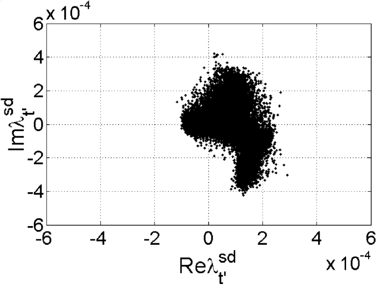
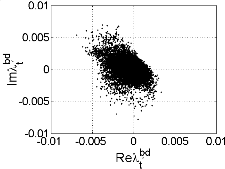
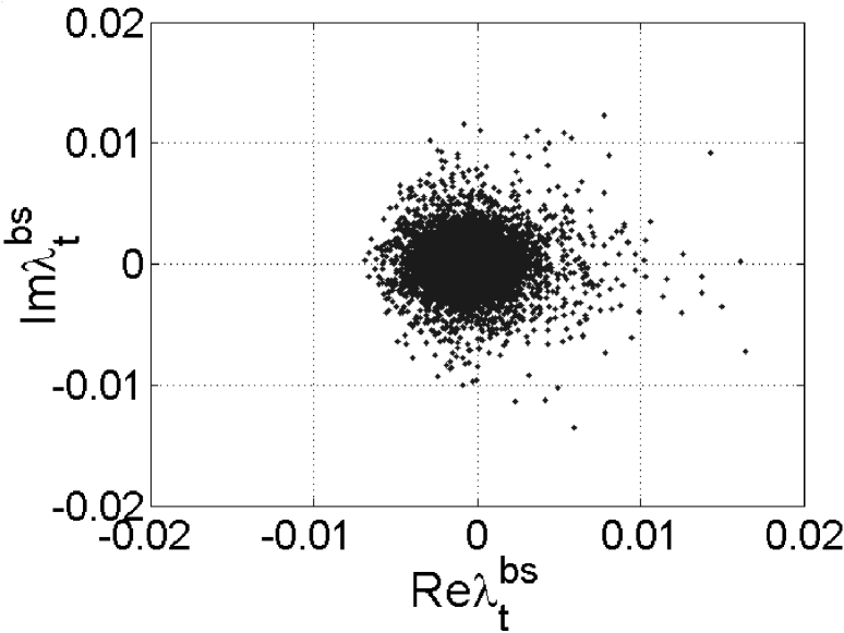
Figure 2: Scatter plot of the New Physics parameters (a) $\lambda_{t^{\prime}}^{sd}$, (b) $\lambda_{t^{\prime}}^{bd}$ and (c) $\lambda_{t^{\prime}}^{bs}$ with all the constraints, for $m_{t^{\prime}}=500$ GeV and $m_{b^{\prime}}=470$ GeV.

Our analysis shows that there is very little correlation between the various constraints. This means that each of the parameters is effectively constrained only by a small number of constraints. We now consider each of the parameters and the constraints that influence it most.

1. $\lambda_{t^{\prime}}^{sd}$: The bound on $Im\lambda_{t^{\prime}}^{sd}$ comes mainly from the $B(K^{+}\to\pi^{+}\nu\bar{\nu})$ constraint. The real part, $Re\lambda_{t^{\prime}}^{sd}$, is mainly constrained by $B(K_{L}\to\mu\bar{\mu})_{SD}$. The general shape of $\lambda_{t^{\prime}}^{sd}$ is mainly due to the $\varepsilon_{K}$ constraint.

2. $\lambda_{t^{\prime}}^{bd}$: $|\lambda_{t^{\prime}}^{bd}|$ is mainly constrained by the $\Delta m_{B_{d}}$ constraint. The $a_{\psi K}$ constraint is responsible for the area excluded in the upper–right and lower–left regions in figure 2. We also examined how an improvement in the experimental error for $a_{\psi K}$ will affect the influence of this constraint. As it turns out, the excluded area is almost insensitive to the size of the error, and even an error as low as 0.01 (10 percent of the current error) will have very little effect in the $(Re\lambda_{t^{\prime}}^{bd},Im\lambda_{t^{\prime}}^{bd})$ plane. A change in the central value from 0.8 to 0.7 will have some influence on the excluded area. In general, the higher the central value is, the larger is the excluded area. However, the modifications in the excluded area are in any case not drastic. This means that the coming experimental results for $a_{\psi K}$ are not expected to change the bounds on the fourth–generation flavor parameters in a significant manner.

3. $\lambda_{t^{\prime}}^{bs}$: This parameter is constrained mainly by the $B\to X_{s}\ell^{+}\ell^{-}$ bound, together with the tree–level constraints and the $Z\to b\bar{b}$ constraint. It is little influenced by the $\Delta m_{B_{s}}$ bound. Our bounds for this parameter are better than those previously quoted in the literature, since we use an updated (and stronger) experimental constraint for $B\to X_{s}\ell^{+}\ell^{-}$.

A good way to compare the four–generation model to the SM is to look at the predictions given by the two models for various quantities. The results are summarized in table 3.

	$B(K_{L}\to\mu\bar{\mu})_{SD}$	$B(K_{L}\to\pi^{0}\nu\bar{\nu})$	$B(K^{+}\to\pi^{+}\nu\bar{\nu})$	$B(B\to X_{s}\ell^{+}\ell^{-})$
experiment	$\leq 3.75\times 10^{-9}$	$\leq 5.9\times 10^{-7}$	$\leq 5.07\times 10^{-10}$	$\leq 1\times 10^{-5}$
SM	$[0.4,1.4]\times 10^{-9}$	$[1.7,5.6]\times 10^{-11}$	$[4.7,11.0]\times 10^{-11}$	$[3.8,13]\times 10^{-6}$ (ref. [25])
four–generations	$\leq 1.18\times 10^{-8}$	$\leq 4.2\times 10^{-9}$	$\leq 6.7\times 10^{-10}$	-
VDQ	$\leq 2.4\times 10^{-8}$	$\leq 4\times 10^{-10}$	$\leq 8.3\times 10^{-10}$	$\leq 2.5\times 10^{-3}$
	$\Delta m_{B_{s}}\,[ps^{-1}]$	$|M_{12}^{D}|\,$[GeV]	$\frac{a_{SL}}{{\left(\Gamma_{12}/M_{12}\right)}^{SM}}$
experiment	$\geq 15$	$\leq 8.2\times 10^{-14}$	$[-5.84,+5.05]$ [26, 27, 28, 29]
SM	$[15,32]$	$\sim 10^{-17}$ to $10^{-16}$	$[0.04,0.26]$ (Ref. [30])
four–generations	$[12,28]$	$\leq 2.7\times 10^{-15}$	$[-1.3,+1.8]$
VDQ	$[15,32]$	-	$[-0.47,+0.28]$

Table 3: Predictions for different quantities in the SM and in the four–generation model compared to the experimental bounds, taken at two sigma. The category of ’favored range’ in the four–generation model refers to the range that contains 95$\%$ of the data points.

We give here several notes regarding these predictions:

1. The predictions for $|M_{12}^{D}|$, $B(K_{L}\to\mu\bar{\mu})_{SD}$, $B(K^{+}\to\pi^{+}\nu\bar{\nu})$ and $B(K_{L}\to\pi^{0}\nu\bar{\nu})$ in the four–generation model can be significantly higher then the SM predictions. In the cases of $B(K_{L}\to\mu\bar{\mu})_{SD}$ and $B(K^{+}\to\pi^{+}\nu\bar{\nu})$ they can span the entire range implied from the experimental constraints.

2. The CP asymmetry in semi–leptonic decays is approximately given by the model–independent expression [30]

   $$\frac{a_{SL}}{{\left(\Gamma_{12}/M_{12}\right)}^{SM}}=\frac{\sin 2\theta_{d}}{|M_{12}/M_{12}^{SM}|}$$ (23)

   The experimental bound on this quantity is obtained by calculating the world–average of $a_{SL}=(0.2\pm 1.4)\times 10^{-2}$ from [26, 27, 28, 29], and taking into account the theoretical predictions for ${\left(\Gamma_{12}/M_{12}\right)}^{SM}\approx-(0.79\pm 0.27)\times 10^{-2}$ (by an updated scan according to the data in ref. [30]). Although our scan improves the bounds which were obtained in [4], the four–generation model prediction for this quantity can still be about an order of magnitude higher than that of the SM. Also, this quantity in the four generation model may have a different sign from that predicted by the SM. The four–generation prediction for $a_{SL}$ is quite far from the current experimental bound. In case the experimental bound improves by about a factor of 3 for the upper bound and 4.5 for the lower bound, this bound will become significant in the analysis.

3. Taking all constraints at two sigma, the $a_{\psi K}$ prediction in the four–generation model covers the entire range allowed by the $B\to\psi K$ constraint. The SM prediction covers the range $0.6\leq a_{\psi K}\leq 0.95$. However, the difference between the SM and the four–generation model regarding this quantity can be clearly seen if we perform the scan without including the $B\to\psi K$ constraint. Then the four–generation model allows the range $-1\leq a_{\psi K}\leq 1$, while the SM allowed range is only $0.4\leq a_{\psi K}\leq 0.95$. Still, from the latest experimental results it is clear that the value of $a_{\psi K}$ lies at the higher part of the allowed range, so this information is of limited impact.

4. The $\Delta m_{B_{s}}$ prediction in the four–generation model is similar to the prediction of the SM. This means that detection of $\Delta m_{B_{s}}$ outside the SM range will be a major problem not only for the SM but also for the four generation model.

2.7 The case of $m_{t^{\prime}}=200$ GeV, $m_{b^{\prime}}=170$ GeV

In this case, the bounds that are obtained for the mixing parameters are significantly weaker than for the case of $m_{t^{\prime}}=500$ GeV, $m_{b^{\prime}}=470$ GeV. The fact that the strongest effects are obtained for the heavier mass of $t^{\prime}$ can be explained as follows. Roughly speaking, the diagrams that we consider put bounds on terms of the form $\lambda_{t^{\prime}}^{lm}y_{i}(x_{t^{\prime}})$, where $y_{i}(x_{t^{\prime}})$ is some Inami–Lim function. Since $y_{i}(x_{t^{\prime}})$ grows with $x_{t^{\prime}}\equiv{m_{t^{\prime}}}^{2}/{m_{W}}^{2}$, the heavier the mass is, the stronger is the bound on the parameter $\lambda_{t^{\prime}}^{lm}$.

The histograms for the phase $\phi_{13}$ and the angles $\sin\theta_{14}$ and $\sin\theta_{24}$ are qualitatively the same as for the case $m_{t^{\prime}}=500$. The resulting ranges of the new mixing angles and phases are given by:

$$0 \lesssim\phi_{13}\lesssim\frac{\pi}{2},$$

$$0 \lesssim\sin\theta_{14}\lesssim 0.051\ ,$$

$$0 \lesssim\sin\theta_{24}\lesssim 0.056\ ,$$ (24)

$$0 \lesssim\sin\theta_{34}\lesssim 0.3\ .$$

The remaining new phases ($\phi_{14}$ and $\phi_{24}$) can again take the entire scanned range.

The bounds on the New Physics parameters $\lambda_{t^{\prime}}^{bd}$, $\lambda_{t^{\prime}}^{bs}$ and $\lambda_{t^{\prime}}^{sd}$ are presented in figure 3. In this case, $\lambda_{t^{\prime}}^{bs}$ is constrained mainly by the tree–level decay processes, $Z\to b\bar{b}$ and unitarity, and not by $B\to X_{s}\ell^{+}\ell^{-}$ as in the case of $m_{t^{\prime}}=500$ GeV. Other than that, one can see that the bounds for the cases of $m_{t^{\prime}}=500$ GeV and $m_{t^{\prime}}=200$ GeV are qualitatively the same, with obvious numerical differences.

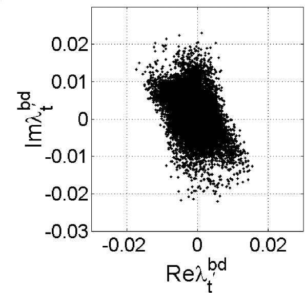
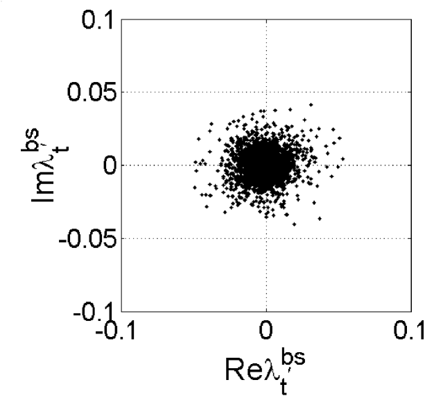
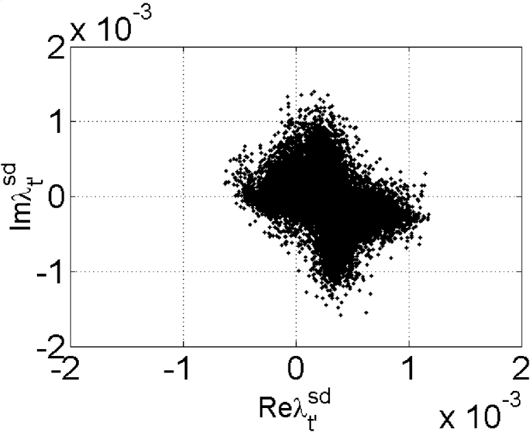
Figure 3: Scatter plot of the New Physics parameters (a) $\lambda_{t^{\prime}}^{bd}$, (b) $\lambda_{t^{\prime}}^{bs}$ and (c) $\lambda_{t^{\prime}}^{sd}$ with all the constraints, for $m_{t^{\prime}}=200$ GeV and $m_{b^{\prime}}=170$ GeV.

The predictions for various quantities in the case of $m_{t^{\prime}}=200$ GeV, $m_{b^{\prime}}=170$ GeV are quite close to the those in the case of $m_{t^{\prime}}=500$ GeV, $m_{b^{\prime}}=470$ (table 3). Basically this means that the allowed ranges of the four–generation model for these quantities is almost independent of the new quark masses.

3 Vector–like Down–type Quarks (VDQ)

3.1 Background

We consider a model in which a single VDQ is added to the SM. Vector–like quarks transform as triplets under the ${SU(3)}_{C}$ symmetry, and both their left–handed and right–handed components transform as singlets under the ${SU(2)}_{L}$ symmetry. VDQs are predicted by various extensions of the SM, such as grand unified theories based on the $E_{6}$ Lie algebra. Also, as explained in section 1, models with VDQ exhibit interesting features such as the violation of CKM unitarity and the related appearance of FCNC contributions at tree–level, and the appearance of additional CP violating phases.

The constraints we consider in our analysis are the following: charged–current tree–level decays, the branching ratios $B(B\to X_{s}\ell^{+}\ell^{-}),B(K^{+}\to\pi^{+}\nu\bar{\nu})$ and $B(K_{L}\to\mu\bar{\mu})_{SD}$, the mass differences $\Delta m_{B_{d}}$ and $\Delta m_{B_{s}}$, the CP violating parameters $\varepsilon_{K}$, $\frac{\varepsilon\prime}{\varepsilon}$ and $a_{\psi K}$, and precision electroweak measurements related to the $Z\bar{b}b$ coupling. The scan procedure that we use is similar to that used for the four generation model.

This model was previously studied in the literature (see [31] and references therein). Regarding $R_{b}$ and $A^{b}_{FB}$ (the forward–backward asymmetry of the $b$ quark) in this model, see [32]. Recent works similar to the one presented here were performed by [33]. We update the experimental bounds used there, taking into account the new results from Belle and BABAR collaborations regarding the $B\to\psi K$ measurements. We also present the predictions of this model for various observables and compare them to the predictions of the SM. While this paper was in final stages of writing, another article [34] was published on this subject.

3.2 The model

We consider a single VDQ, denoted $b^{\prime}$, added to the SM. This means that the mass matrix in the down sector is now $4\times 4$, and it is diagonalized by a $4\times 4$ matrix $V$. The down sector charged–current interactions depend on the $3\times 4$ upper submatrix of $V$, which plays the role of the CKM matrix, but are otherwise unchanged. The neutral–current interactions are given in this model by

$$\mathcal{L}_{NC}={g\over 2\cos{\theta_{W}}}Z^{\mu}(\overline{\mathcal{U}^{M}_{L}}\gamma_{\mu}\mathcal{U}^{M}_{L}-\overline{\mathcal{D}^{M\alpha}_{L}}\gamma_{\mu}U_{\alpha\beta}\mathcal{D}^{M\beta}_{L}-2\sin^{2}{\theta_{W}}J^{EM}_{\mu})\ ,$$ (25)

where a sum over repeated indices is implied ($\alpha,\beta=d,s,b$), and we used the definitions

$$\mathcal{U}\equiv\left(\begin{array}[]{l}u\\ c\\ t\\ \end{array}\right),\ \ \mathcal{D}\equiv\left(\begin{array}[]{l}d\\ s\\ b\\ \end{array}\right),\ \ U_{\alpha\beta}\equiv\sum_{i=1}^{3}V^{*}_{i\alpha}V_{i\beta}=\delta_{\alpha\beta}-V^{*}_{4\alpha}V_{4\beta}\ .$$ (26)

In eq. (25), $J^{EM}_{\mu}$ is the electromagnetic current, which contains also terms with the new quark $b^{\prime}$. Note that eq. (25) contains FCNC. In all the processes we consider, the leading New Physics contributions come from the tree–level FCNC that appear in eq. (25) through the quantities $U_{\alpha\beta}$. These New Physics contributions usually compete with contributions coming from SM loop processes. Other New Physics effects, due to $b^{\prime}$ quarks in loop diagrams, are naturally highly suppressed compared to the tree–level contributions, and can be safely neglected. We can thus view this model at low energies as having the same particle content and interactions as the SM (completely ignoring the extra $b^{\prime}$ quark), but having a non unitary CKM matrix.

Note that the quantities $U_{bs}$, $U_{bd}$ and $U_{sd}$ play two important roles. First, they indicate the amount by which the three–generation CKM matrix deviates from unitarity. Second, they represent the strength of the new contributions to FCNC. These quantities play the same role as $-\lambda_{t^{\prime}}^{ij}$ in the four–generation model.

The matrix $V$ is not a general unitary matrix; some of the phases in it can be removed by change of basis. It can be parameterized by nine parameters: six mixing angles and three phases. All these parameters appear also in the upper $3\times 4$ submatrix. As in the four–generation model, we use the specific parameterization of [5] for the $4\times 4$ matrix $V$, in order to incorporate all the correlations in our analysis. The mixing angles are again referred to as $\theta_{12},\theta_{13},\theta_{23},\theta_{14},\theta_{24}$ and $\theta_{34}$, and the phases as $\phi_{13},\phi_{14}$ and $\phi_{24}$.

3.3 The constraints

The constraints obtained from the tree–level decays are the same as in the four–generation model, described in section 2.3. The expression for $B(B\to X_{s}\ell^{+}\ell^{-})$ in the VDQ model is given by eq. (19), with the coefficients $C_{2}$, $\tilde{C}_{9}$ and $\tilde{C}_{10}$ taken as

$$\begin{split}C_{2}&=1-\frac{U_{bs}}{\lambda_{t}^{bs}},\\ \tilde{C}_{9}&=\frac{8}{9}\ln\left(\frac{M_{W}}{m_{B}}\right)\left(1-\frac{U_{bs}}{\lambda_{t}^{bs}}\right)+\frac{Y_{0}(x_{t})}{\sin^{2}\theta_{W}}-4Z_{0}(x_{t})+\left(\frac{1}{\sin^{2}\theta_{W}}-4\right)C_{U2Z}\frac{U_{bs}}{\lambda_{t}^{bs}},\\ \tilde{C}_{10}&=-\frac{Y_{0}(x_{t})+C_{U2Z}\frac{U_{bs}}{\lambda_{t}^{bs}}}{\sin^{2}\theta_{W}}.\end{split}$$ (27)

The coefficient $C_{7\gamma}$ remains unchanged.

The expressions for the remaining constraints are very similar to those used in the four generation case. They are taken as in [33], but with the input parameters given in tables 1 and 2. For the $\varepsilon^{\prime}\over\varepsilon$ constraint we use only the ranges of the parameters given in [35].

3.4 Numerical results

The numerical scan is performed in the same way as in the four generation case. The results of the scan show that the CP violating phases $\phi_{14}$ and $\phi_{24}$ can be in the entire scanned range (from 0 to $2\pi$). Yet, as in the four generation case, the phase $\phi_{13}$ has a restricted range, $0\lesssim\phi_{13}\lesssim\pi$. This results agrees with [33]. A histogram for this phase can be seen in figure 4. The mixing angles $\theta_{14}$ and $\theta_{24}$ also have restricted ranges:

$$0\lesssim\sin\theta_{14}\lesssim 0.011\ ,$$

$$0\lesssim\sin\theta_{24}\lesssim 0.011\ .$$ (28)

\psfragscanon\psfrag{str04}[t][t]{$\phi_{13}$ (radians)}\psfrag{x01}[t][t]{1}\psfrag{x02}[t][t]{2}\psfrag{x03}[t][t]{3}\psfrag{x04}[t][t]{4}\psfrag{x05}[t][t]{5}\psfrag{x06}[t][t]{6}\psfrag{v01}[r][r]{0}\psfrag{v02}[r][r]{2000}\psfrag{v03}[r][r]{4000}\psfrag{v04}[r][r]{6000}\psfrag{v05}[r][r]{8000}\psfrag{v06}[r][r]{10000}\psfrag{v07}[r][r]{12000}\psfrag{v08}[r][r]{14000}\psfrag{origin1}[lb][lb]{\begin{picture}(1.0,0.78871)\end{picture}}\includegraphics[width=129.06111pt]{vldt_phi13.eps}

\psfragscanon\psfrag{str01}[t][t]{$\sin\theta_{14}$}\psfrag{x01}[t][t]{0}\psfrag{x02}[t][t]{0.01}\psfrag{x03}[t][t]{0.02}\psfrag{x04}[t][t]{0.03}\psfrag{x05}[t][t]{0.04}\psfrag{v01}[r][r]{0}\psfrag{v02}[r][r]{5000}\psfrag{v03}[r][r]{10000}\psfrag{v04}[r][r]{15000}\psfrag{v05}[r][r]{20000}\psfrag{v06}[r][r]{25000}\psfrag{origin1}[lb][lb]{\begin{picture}(1.0,0.78871)\end{picture}}\includegraphics[width=129.06111pt]{vldt_theta14.eps}

\psfragscanon\psfrag{str04}[t][t]{$\sin\theta_{24}$}\psfrag{x01}[t][t]{0}\psfrag{x02}[t][t]{0.01}\psfrag{x03}[t][t]{0.02}\psfrag{x04}[t][t]{0.03}\psfrag{x05}[t][t]{0.04}\psfrag{v01}[r][r]{0}\psfrag{v02}[r][r]{0.5}\psfrag{v03}[r][r]{1}\psfrag{v04}[r][r]{1.5}\psfrag{v05}[r][r]{2\begin{picture}(0.0,0.0)\put(0.5,1.5){$\times 10^{4}$}\end{picture}}\psfrag{origin1}[lb][lb]{\begin{picture}(1.0,0.78871)\end{picture}}\includegraphics[width=129.06111pt]{vldt_theta24.eps}

Figure 4: Histograms of (a) $\phi_{13}$, (b) $\sin\theta_{14}$ and (c) $\sin\theta_{24}$ for 75,000 data points in the VDQ model

The restricted regions are due to combinations of several constraints. For example, the restricted range of $\sin\theta_{24}$ is mainly due to the correlated effect of the $K_{L}\to\mu\bar{\mu}$ and $\frac{\varepsilon^{\prime}}{\varepsilon}$ constraints. The remaining phases, $\phi_{24}$ and $\phi_{14}$ can be in all the scanned range. The mixing angle $\theta_{34}$ can be in the range $0\lesssim\sin\theta_{34}\lesssim 0.12$ (see [33]).

We now examine the allowed regions of the parameters $U_{sd}$, $U_{bd}$ and $U_{bs}$, which represent the New Physics contributions in this model. Their scatter plots are given in Figure 5. They are in very good agreement with the results of [33], except for changes which are related to the recent $a_{\psi K}$ and $B\to X_{s}\ell^{+}\ell^{-}$ measurements.

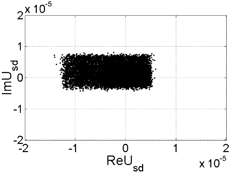
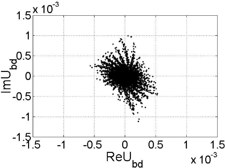
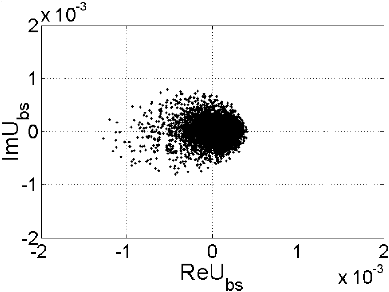
Figure 5: Scatter plot of the New Physics parameters (a) $U_{sd}$, (b) $U_{bd}$ and (c) $U_{bs}$ with all the constraints.

As in the case of the four generations, also in this case each of the parameters is effectively constrained only by a small number of constraints. We now consider each of the parameters:

1. $U_{sd}$: The bound on $ImU_{sd}$ comes mainly from the $\varepsilon^{\prime}\over\varepsilon$ constraint. The real part, $ReU_{sd}$, is mainly constrained by $B(K_{L}\to\mu\bar{\mu})_{SD}$.

2. $U_{bd}$: $|U_{bd}|$ is mainly constrained by the $\Delta m_{B_{d}}$ constraint. The $a_{\psi K}$ constraint is responsible for the area excluded in the upper–right and lower–left regions in figure 5. We examined how an improvement in the experimental error for $a_{\psi K}$ will affect this constraint. As in the four generation case, the results show that the excluded area is almost insensitive to the size of the error, and there is little sensitivity also to the central value. This means that the coming experimental results for $a_{\psi K}$ are not expected to change the bounds on the flavor parameters of the VDQ model in a significant manner.

3. $U_{bs}$: This parameter is mainly constrained by the $B\to X_{s}\ell^{+}\ell^{-}$ bound. It is little influenced even by $\Delta m_{B_{s}}$. The bounds we obtain are better than those obtained in previous works [33] due to the improved experimental bound (see table 1) that we use.

The last step in comparing this model to the SM is to consider the predictions given by the two models for various quantities (see table 3). We give here several notes regarding these predictions:

1. The predictions for $B(K_{L}\to\mu\bar{\mu})_{SD}$, $B(K^{+}\to\pi^{+}\nu\bar{\nu})$ and $B(K_{L}\to\pi^{0}\nu\bar{\nu})$ in the VDQ model can be substantially higher than the predictions of the SM. The prediction for $B(K_{L}\to\mu\bar{\mu})_{SD}$ can actually span the entire range allowed by the experimental constraints.

2. The prediction for $B(B\to X_{s}\ell^{+}\ell^{-})$ in the VDQ model can reach the current experimental bound. This is in contrast to the prediction in the case of low $a_{\psi K}$ values, as presented in [33]. In a similar way, the predictions for $B(B\to X_{d}\ell^{+}\ell^{-})$ are also large in this model.

3. The scan results for the CP asymmetry in semi–leptonic decays (as given in table 3) improve the bounds which were obtained in [4]. Note that the prediction in the VDQ model may have a different sign than the SM prediction. In order for the $a_{SL}$ constraint to have a significant impact on the parameters of the VDQ model, the experimental results must improve by about an order of magnitude. Such an improvement is not expected in the near future.

4. The behavior of the predictions for $a_{\psi K}$ are similar to the four generation case. When taking all constraints at two sigma, the results for the SM and for the VDQ model are practically the same. But when performing the scan without including the $B\to\psi K$ constraint, the VDQ model allows the entire range for $a_{\psi K}$, while the SM allows only a very restricted range. Still, from the latest experimental results it is clear that the value of $a_{\psi K}$ lies at the higher part of the allowed range, so this information is of limited interest.

5. As in the four generation case, the $\Delta m_{B_{s}}$ prediction in the VDQ model is similar to the prediction of the SM. This again means that detection of $\Delta m_{B_{s}}$ outside the predictions of the SM will be problematic also in the VDQ model.

4 Discussion and Conclusions

We considered constraints from tree–level decays, electroweak precision measurements, the decay $Z\to b\bar{b}$, rare $K$ and $B$ decays, CP violating parameters in the $K$ and in the $B$ systems and mass differences in various neutral meson systems in order to obtain bounds and predictions for the four generation model and for the VDQ model. The constraint on the four generation model from $Z\to b\bar{b}$ proves to be very powerful, as it excludes a significant portion of the parameter space. Improvement in the $B(B\to X_{s}\ell^{+}\ell^{-})$ measurement provides better bounds on the New Physics parameters in both models. The new experimental data for $a_{\psi K}$ also affects our results, causing the analysis for the VDQ model to be quite different from the results of [33]. Furthermore, according to our analysis additional improvement of this measurement is expected to have only minor effects on both the four generation and the VDQ models. Improvement of the bounds for these models can thus be expected mainly by better determination of other measurements such as $B(B\to X_{s}\ell^{+}\ell^{-})$, $B(K^{+}\to\pi^{+}\nu\bar{\nu})$, $a_{SL}$, and $\Delta m_{B_{s}}$. Of course, both of the models can never be strictly excluded by flavor physics, since by proper adjustment of the new parameters one can always reduce them to the SM. In the four–generation model, this can be done by taking the mixing between the fourth generation and the three SM generations to be very small ($\sin\theta_{34},\sin\theta_{14},\sin\theta_{24}\to 0$). The result is decoupling of the fourth generation from the other three. In the VDQ model, this can be achieved by taking the mass of the new quark to be very high. Since the new mixing angles result from the diagonalization of the mass matrix, they are roughly given by $\theta_{i4}\approx\frac{m_{i}}{m_{4}}$, so by taking $m_{4}\gg m_{i}$ we can make all the new mixing angles vanish.

We find that the two models which we consider share many common features. They both contain new sources of CP violation that arise from a $4\times 4$ CKM-like matrix, and both predict for various observables values that can be higher than those predicted by the SM. Another aspect that the two models share is that they both introduce new FCNC contributions. In both models these new FCNC contributions are naturally small, though they can still be larger than the SM contributions. This was shown to lead to substantial increase in the values the two models predict for various quantities, compared to the SM predictions. Despite these (and other) similarities between the four–generation and the VDQ models, there are also significant differences between them. One of the differences is related to the fact that the mechanism that introduces the new FCNC sources is not the same in the two models. The new FCNC contributions in the four–generation model come from loop diagrams with the new fermions in the loop. These diagrams are roughly proportional to ${\left(\frac{m_{t^{\prime}}}{M_{W}}\right)}^{2}\approx O(10)$. In the VDQ model, on the other hand, the leading new FCNC contributions come from tree–level diagrams, with a coefficient of $C_{U2Z}\approx O(100)$ (see e.g. [33]). Thus the new contributions for the FCNC processes in the two models differ by an order of magnitude.

This order–of–magnitude difference leads to various effects. One of these regards the unitarity relation $\lambda_{u}^{bd}+\lambda_{c}^{bd}+\lambda_{t}^{bd}+\lambda_{t^{\prime}}^{bd}=0$ in the four–generation model, or $\lambda_{u}^{bd}+\lambda_{c}^{bd}+\lambda_{t}^{bd}-U_{bd}=0$ in the VDQ model. As was already discussed in the literature (see e.g. [4] and references therein), in both cases one gets unitarity quadrangles instead of the unitarity triangle that exist in the SM. When examining the results of the numerical scan (see table 4), it is clear that the possible shapes that the unitarity quadrangle can take is very different in the two models. The parameter $r$ is defined by

$$r\equiv\left\{\begin{array}[]{l}\frac{\lambda_{t^{\prime}}^{bd}}{\lambda_{t}^{bd}}\ \ \ \ {\rm{four\ generation\ model}}\\ \\ \frac{U_{bd}}{\lambda_{t}^{bd}}\ \ \ \ {\rm{VDQ\ model}.}\end{array}\right.$$ (29)

Model	$\beta$ (degrees)	$r$
SM	22 - 33	0
four–generations ($m_{t^{\prime}}=500GeV$)	0 - 57, 281-360	$\lesssim 3.5$
four–generations ($m_{t^{\prime}}=200GeV$)	0 - 92, 230-360	$\lesssim 70$
VDQ	2 - 38	$\lesssim 0.16$

Table 4: Allowed ranges of various parameters related to the unitarity quadrangle, when all constraints are taken at two sigma. $r$ is defined in eq. (29).

One can see that in the four–generation model, $\lambda_{t^{\prime}}^{bd}$ can be significantly larger than the corresponding SM quantity $\lambda_{t}^{bd}$ (up to a factor of 3.5 for $m_{t^{\prime}}=500$ GeV and a factor of 70 for $m_{t^{\prime}}=200$ GeV), while in the VDQ model $U_{bd}$ is only allowed to be about 15$\%$ of $\lambda_{t}^{bd}$. This difference can be traced back to the order–of–magnitude difference between the new FCNC contributions in the two models. As a result of this, also the ranges of the angle $\beta$ are significantly different in the two models. While in the VDQ model the unitarity quadrangle can be only slightly modified compared to the SM triangle (due to the limited size of r and $\beta$), in the four–generation model the shape of the unitarity quadrangle can be completely different than that of the SM unitarity triangle (especially in the $m_{t^{\prime}}=200$ GeV case).

References

• [1] Particle Data Group (D. E. Groom et al.), Eur. Phys. J. C 15, 1 (2000).
• [2] M. Maltoni, V. A. Novikov, L. B. Okun, A. N. Rozanov and M. I. Vysotsky, Phys. Lett. B476 107, (2000) [hep-ph/9911535];
V. A. Novikov, L. B. Okun, A. N. Rozanov and M. I. Vysotsky, hep-ph/0111028.
• [3] T. Hattori, T. Hasuike and S. Wakaizumi, Phys. Rev. D 60, 113008 (1999) [hep-ph/9908447].
• [4] G. Eyal and Y. Nir, JHEP 9909, 013 (1999) [hep-ph/9908296].
• [5] F. J. Botella and L. L. Chau, Phys. Lett. B 168, 97 (1986).
• [6] T. Affolder et al. [CDF Collaboration], Phys. Rev. Lett.  84, 835 (2000) [hep-ex/9909027];
S. Abachi et al. [D0 Collaboration], Phys. Rev. Lett.  78, 3818 (1997) [hep-ex/9611021].
• [7] A. J. Buras, hep-ph/0101336.
• [8] M. Bargiotti et al., Riv. Nuovo Cim.  23N3, 1 (2000) [hep-ph/0001293].
• [9] [LEP Collaborations], hep-ex/0103048.
• [10] G. D’Ambrosio, G. Isidori and J. Portoles, Phys. Lett. B 423, 385 (1998) [hep-ph/9708326].
• [11] D. Ambrose et al. [E871 Collaboration], Phys. Rev. Lett.  84, 1389 (2000).
• [12] E787 Collaboration, hep-ex/0111091.
• [13] K. Abe et al. [Belle Collaboration], hep-ex/0107072.
• [14] L. Iconomidou-Fayard [the NA48 Collaboration], hep-ex/0110028.
• [15] B. Aubert et al. [BABAR Collaboration], Phys. Rev. Lett.  87, 091801 (2001) hep-ex/0107013.
• [16] K. Abe et al. [Belle Collaboration], Phys. Rev. Lett.  87, 091802 (2001) hep-ex/0107061.
• [17] T. Affolder et al. [CDF Collaboration], Phys. Rev. D 61, 072005 (2000) [hep-ex/9909003].
• [18] G. Raz, hep-ph/0205113.
• [19] T. Inami and C. S. Lim, Prog. Theor. Phys.  65, 297 (1981) [Erratum-ibid.  65, 1772 (1981)].
• [20] G. Buchalla, A. J. Buras and M. E. Lautenbacher, Rev. Mod. Phys.  68, 1125 (1996) [hep-ph/9512380].
• [21] L. Lellouch and C. J. Lin [UKQCD Collaboration], Phys. Rev. D 64, 094501 (2001) hep-ph/0011086.
• [22] The BaBar Physics Book, eds. P. F. Harrison and H. R. Quinn, SLAC-R-504 (1998).
• [23] B. Aubert et al. [BABAR Collaboration], hep-ex/0203007.
• [24] J. Bernabeu, A. Pich and A. Santamaria, Nucl. Phys. B 363, 326 (1991).
• [25] A. Ali, G. Hiller, L. T. Handoko and T. Morozumi, Phys. Rev. D 55, 4105 (1997) [hep-ph/9609449].
• [26] R. Barate et al. [ALEPH Collaboration], Eur. Phys. J. C 20, 431 (2001).
• [27] B. Aubert et al. [BABAR Collaboration], hep-ex/0107059.
• [28] D. E. Jaffe et al. [CLEO Collaboration], Phys. Rev. Lett.  86, 5000 (2001) [hep-ex/0101006].
• [29] G. Abbiendi et al. [OPAL Collaboration], Eur. Phys. J. C 12, 609 (2000) [hep-ex/9901017].
• [30] S. Laplace, Z. Ligeti, Y. Nir and G. Perez, hep-ph/0202010.
• [31] F. del Aguila and J. Cortes, Phys. Lett. B 156, 243 (1985);
G. C. Branco and L. Lavoura, Nucl. Phys. B 278, 738 (1986);
Y. Nir and D. J. Silverman, Phys. Rev. D 42, 1477 (1990);
D. Silverman, Phys. Rev. D 45, 1800 (1992);
V. Barger, M. S. Berger and R. J. Phillips, Phys. Rev. D 52, 1663 (1995) [hep-ph/9503204].
• [32] D. Choudhury, T. M. Tait and C. E. Wagner, Phys. Rev. D 65, 053002 (2002) [arXiv:hep-ph/0109097].
• [33] G. Barenboim, F. J. Botella and O. Vives, Phys. Rev. D 64, 015007 (2001) [hep-ph/0012197] ;
G. Barenboim, F. J. Botella and O. Vives, Nucl. Phys. B 613, 285 (2001) G. Barenboim, F. J. Botella and O. Vives, [hep-ph/0105306].
• [34] D. Hawkins and D. Silverman, hep-ph/0205011.
• [35] A. J. Buras and L. Silvestrini, Nucl. Phys. B 546, 299 (1999) [hep-ph/9811471].