Effects of neutrino oscillation on supernova neutrino: inverted mass hierarchy

1 Introduction

Neutrino mixing and mass spectrum are the keys to probe new physics beyond the standard model of particle physics. Some of the neutrino oscillation parameters have been revealed dramatically by the observation of the atmospheric neutrino [1] and the solar neutrino [2, 3, 4, 5, 6]. Recently the first results of the KamLAND experiment have confirmed the Large Mixing Angle (LMA) solution of the solar neutrino problem [7]. An upper bound on $\mathchar 28946\relax_{13}$ has also been obtained from CHOOZ experiment [8] and a lower bound is expected to obtained from single and double beta decay experiments [9]. But there still remain some ambiguities in the properties of neutrinos: the mass hierarchy, i.e., normal or inverted and the magnitude of $\mathchar 28946\relax_{13}$. Current status is reviewed by many authors [10, 11, 12, 13].

In such present situation, much attention have been paid to another neutrino source, supernova. This is a completely different system from sun, atmosphere, accelerator, and reactor in regard to neutrino energy, flavor of produced neutrinos, propagation length and so forth. Then neutrino emission from a supernova is expected to give valuable information that can not be obtained from neutrinos from other sources. In fact, pioneering observations of neutrinos from SN1987A [14, 15] contributed significantly to our knowledge of the fundamental properties of neutrinos [16, 17, 18]. Especially there have been many studies about the implication for the mass hierarchy from the observed neutrino events and the inverted hierarchy is disfavored if $\sin^{2}{\mathchar 28946\relax_{13}}$ is rather large ($>10^{-4}$) [19, 20, 21]. Here, normal and inverted mass hierarchies are the mass pattern $m_{3}\gg m_{2}>m_{1}$ and $m_{2}>m_{1}\gg m_{3}$, respectively. In our notation $\mathchar 28929\relax m^{2}_{ij}=m^{2}_{j}-m^{2}_{i}$, $\mathchar 28929\relax m^{2}_{12}$ and $\mathchar 28929\relax m^{2}_{13}\sim\mathchar 28929\relax m^{2}_{23}$ are the mass squared differences which are related with the solutions of the solar and atmospheric neutrino problems, respectively. There have also been studies to try to extract the unknown neutrino properties from future supernova [22, 23, 24, 25, 26, 27].

In this paper, we calculate numerically the effects of neutrino oscillation on supernova neutrino, extending our previous study [27] where all analyses are performed with normal mass hierarchy, and investigate the possibility to identify the mass hierarchy and to probe the neutrino oscillation parameters $\mathchar 28946\relax_{13}$ by the observation of the neutrinos from the next galactic supernova. We use the original neutrino spectra from supernova based on a realistic supernova model and the density profile of the progenitor star based on a realistic presupernova model. Since uncertainties of the original neutrino spectra are important in this analysis, we estimate the effect of them on our analysis. The Earth matter effect is also discussed, which have already been studied in the case of normal hierarchy in our previous papers [29, 30].

This paper is organized as follows. In section II we summarize the properties of supernova neutrino briefly. The method of analysis is described and the results are shown in section III. We discuss some ambiguities in the basis of our study and summarize our results in section IV.

2 Supernova Neutrino

Here we summarize the properties of supernova neutrino. For details, see, for example, a review by Suzuki[34]. Almost all of the binding energy of the neutron star,

$$E_{\rm b}\simeq\frac{GM_{\rm NS}^{2}}{R_{\rm NS}}\simeq 3\times 10^{53}{\rm erg}\left(\frac{M_{\rm NS}}{M_{\odot}}\right)^{2}\left(\frac{10{\rm km}}{R_{\rm NS}}\right),$$ (2.1)

is radiated away as neutrinos. Here $G$, $M_{\rm NS}$ and $R_{\rm NS}$ are the gravitational constant, the mass and radius of the neutron star, respectively. Due to the difference of interaction strength, average energies are different between flavors. Although quantitative estimate of the difference is difficult, it is qualitatively true that $\langle E_{\mathchar 28951\relax_{e}}\rangle<\langle E_{\bar{\mathchar 28951\relax}_{e}}\rangle<\langle E_{\mathchar 28951\relax_{x}}\rangle$. Here $\mathchar 28951\relax_{x}$ means $\mathchar 28951\relax_{\mathchar 28950\relax},\mathchar 28951\relax_{\mathchar 28956\relax}$ and their antineutrinos. These differences are essential in this paper.

We use a realistic model of a collapse-driven supernova by the Lawrence Livermore group[36] to calculate the neutrino luminosities and energy spectra, as we did in our previous paper [27]. The average energy of each flavor is:

$$\langle E_{\mathchar 28951\relax_{e}}\rangle\simeq 13{\rm MeV},\;\;\langle E_{\bar{\mathchar 28951\relax}_{e}}\rangle\simeq 16{\rm MeV},\;\;\langle E_{\mathchar 28951\relax_{x}}\rangle\simeq 23{\rm MeV}.$$ (2.2)

Details of this original neutrino spectra are discussed by Totani et al. [37] These neutrinos, which are produced in the high dense region of the iron core, interact with matter before emerging from the supernova. Due to the nonzero masses and the mixing in vacuum among various neutrino flavors, flavor conversions can occur in supernova. When the mixing angle is small, these conversions occur mainly in the resonance layer, where the density is

$$\mathchar 28954\relax_{\rm res}\simeq 1.4\times 10^{6}{\rm g/cc}\left(\frac{\mathchar 28929\relax m^{2}}{1{\rm eV}^{2}}\right)\left(\frac{10{\rm MeV}}{E_{\mathchar 28951\relax}}\right)\left(\frac{0.5}{Y_{e}}\right)\cos{2\mathchar 28946\relax},$$ (2.3)

where $\mathchar 28929\relax m^{2}$ is the mass squared difference, $\mathchar 28946\relax$ is the mixing angle, $E_{\mathchar 28951\relax}$ is the neutrino energy, and $Y_{e}$ is the mean number of electrons per baryon. Since the supernova core is dense enough, there are two resonance points in supernova envelope. One that occurs at higher density is called H-resonance and another is called L-resonance. If the mass hierarchy is normal, both resonances occur in neutrino sector. On the other hand, if the mass hierarchy is inverted, H-resonance occurs in antineutrino sector and L-resonance occurs in neutrino sector. The schematic level crossing diagram for normal and inverted mass hierarchies are shown in Fig. 1.

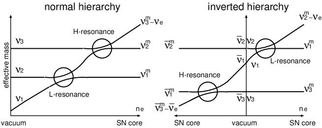
Fig. 1: Schematic level crossing diagram for normal (left) and inverted (right) mass hierarchies. The circles shows the resonance points.

The dynamics of conversions including large mixing case is determined by the adiabaticity parameter $\mathchar 28941\relax$, which depend on the mixing angle and the mass-squared difference between involved flavors:

$$\mathchar 28946\relax_{13}\;{\rm and}\;\mathchar 28929\relax m^{2}_{13}\;{\rm at\;H-resonance},$$ (2.4)

$$\mathchar 28946\relax_{12}\;{\rm and}\;\mathchar 28929\relax m^{2}_{12}\;{\rm at\;L-resonance}.$$ (2.5)

When $\mathchar 28941\relax\gg 1$, the resonance is called ’adiabatic resonance’ and the fluxes of the two involved mass eigenstate are completely exchanged. On the contrary, when $\mathchar 28941\relax\ll 1$, the resonance is called ’nonadiabatic resonance’ and the conversion does not occur. The dynamics of the resonance in supernova is studied in detail by Dighe and Smirnov [22].

3 Method and Results

In this section we describe the method of analysis and show the results.

3.1 Conversion Probabilities

In the framework of three-flavor neutrino oscillation, the time evolution equation of the neutrino wave functions can be written as follows:

$$i\frac{d}{dt}\left(\begin{array}[]{ccc}\mathchar 28951\relax_{e}\\ \mathchar 28951\relax_{\mathchar 28950\relax}\\ \mathchar 28951\relax_{\mathchar 28956\relax}\end{array}\right)=H(t)\left(\begin{array}[]{ccc}\mathchar 28951\relax_{e}\\ \mathchar 28951\relax_{\mathchar 28950\relax}\\ \mathchar 28951\relax_{\mathchar 28956\relax}\end{array}\right),$$ (3.1)

$$H(t)\equiv U\left(\begin{array}[]{ccc}0&0&0\\ 0&\mathchar 28929\relax m^{2}_{12}/2E_{\mathchar 28951\relax}&0\\ 0&0&\mathchar 28929\relax m^{2}_{13}/2E_{\mathchar 28951\relax}\end{array}\right)U^{-1}+\left(\begin{array}[]{ccc}A(t)&0&0\\ 0&0&0\\ 0&0&0\end{array}\right),$$ (3.2)

where $A(t)=\sqrt{2}G_{F}n_{e}(t)$, $G_{F}$ is Fermi constant, $n_{e}(t)$ is the electron number density, and $\mathchar 28929\relax m^{2}_{ij}$ is the mass squared differences. In case of antineutrino, the sign of $A(t)$ changes. Here U is the Cabibbo-Kobayashi-Maskawa (CKM) matrix:

$$U=\left(\begin{array}[]{ccc}c_{12}c_{13}&s_{12}c_{13}&s_{13}\\ -s_{12}c_{23}-c_{12}s_{23}s_{13}&c_{12}c_{23}-s_{12}s_{23}s_{13}&s_{23}c_{13}\\ s_{12}s_{23}-c_{12}c_{23}s_{13}&-c_{12}s_{23}-s_{12}c_{23}s_{13}&c_{23}c_{13}\end{array}\right),$$ (3.3)

where $s_{ij}=\sin{\mathchar 28946\relax_{ij}},c_{ij}=\cos{\mathchar 28946\relax_{ij}}$ for $i,j=1,2,3(i<j)$. We have here put the CP phase equal to zero in the CKM matrix.

By solving numerically these equations along the density profile of progenitor, which is calculated by Woosley and Weaver[39], we obtain conversion probabilities $P(\mathchar 28939\relax\rightarrow\mathchar 28940\relax)$, i.e., probability that $\mathchar 28951\relax_{\mathchar 28939\relax}$ at the center of the supernova becomes $\mathchar 28951\relax_{\mathchar 28940\relax}$ at the surface of the progenitor star.

In our previous paper[27], we assumed the normal mass hierarchy and took four models for neutrino oscillation parameters, the differences being the solution of the solar neutrino problem (LMA or SMA) and the magnitude of $\mathchar 28946\relax_{13}$. Here we take the following values:

$$\sin^{2}{2\mathchar 28946\relax_{12}}=0.84, \mathchar 28929\relax m^{2}_{12}=7\times 10^{-5}{\rm eV}^{2},$$

$$\sin^{2}{2\mathchar 28946\relax_{23}}=1.0, \mathchar 28929\relax m^{2}_{23}=3.2\times 10^{-3}{\rm eV}^{2}.$$ (3.4)

Values of $\mathchar 28946\relax_{12}$ and $\mathchar 28929\relax m^{2}_{12}$ are taken from the global analysis of the solar neutrino observations and the KamLAND experiment[40] and correspond to the LMA solution of the solar neutrino problem while those of $\mathchar 28946\relax_{23}$ and $\mathchar 28929\relax m^{2}_{23}$ are taken from the analysis of the atmospheric neutrino observation[1]. As to $\mathchar 28946\relax_{13}$, we take two fiducial values $\sin^{2}{2\mathchar 28946\relax_{13}}=0.043,\;10^{-6}$ as we did in our previous paper[27]. Later we will discuss the case of the other values. Furthermore, we consider both normal and inverted hierarchy. Consequently, there are four models and we call them normal-LMA-L, normal-LMA-S, inverted-LMA-L and inverted-LMA-S. The last character (L or S) represents the magnitude of $\mathchar 28946\relax_{13}$ (large or small). In our notation, $\mathchar 28929\relax m^{2}_{ij}=m^{2}_{j}-m^{2}_{i}$ so that $\mathchar 28929\relax m^{2}_{13}>0$ in the normal hierarchy case and $\mathchar 28929\relax m^{2}_{13}<0$ in the inverted hierarchy case. Therefore, normal-LMA-L and inverted-LMA-L are different only in the sign of $\mathchar 28929\relax m^{2}_{13}$.

We show in Fig. 2 demonstrations of conversion probabilities. The left figure is the time evolution of $P(e\rightarrow e)$, probability that $\mathchar 28951\relax_{e}$ remains $\mathchar 28951\relax_{e}$, and the right figure is that of $P(\bar{e}\rightarrow\bar{e})$, probability that $\bar{\mathchar 28951\relax}_{e}$ remains $\bar{\mathchar 28951\relax}_{e}$. Four curves for the same model correspond to the neutrino of energy, 5 MeV, 10 MeV, 40 MeV and 70 MeV, respectively. It can be seen that H-resonance and L-resonance occur at the O+Ne+Mg and He layer, respectively. In the neutrino sector, the conversion probabilities for the inverted hierarchy are the same as those for the model normal-LMA-S. This is because the H-resonance is completely nonadiabatic when $\mathchar 28946\relax_{13}$ is very small, as in normal-LMA-S, and this is phenomenologically as if the H-resonance is absent as in the inverted hierarchy case. This logic also applies to why normal-LMA-L, normal-LMA-S and inverted-LMA-S are degenerate in the antineutrino sector, if we consider the H-resonance in the antineutrino sector. These degeneracies are the origins of the degeneracies that appear later in the event rates.

Fig. 2: Time evolution of conversion probabilities $P(e\rightarrow e)$ and $P(\bar{e}\rightarrow\bar{e})$. Four lines of the same marking correspond to neutrino energy, 5MeV, 10MeV, 40MeV, and 70MeV, respectively.

3.2 Event Rates

After obtaining the conversion probabilities, the neutrino fluxes at the Earth are calculated by multiplying the conversion probabilities by the original spectra and the distance factor $1/4\mathchar 28953\relax d^{2}$. Here we take 10 kpc for the distance $d$ between the Earth and the supernova. Further, by multiplying these fluxes by the cross sections of the detection interactions, the detector volume and the detector efficiency, we obtain the event rates at the detectors. Here we consider two detectors: SuperKamiokande (SK) and SNO. Properties of these detectors and cross sections used to calculate event rates are described in our previous paper [27]. Unfortunate accident at SK lessened the detection efficiency at low energy ($<8$ MeV) but this cause negligible effect in the subsequent analysis.

Fig. 3 - 5 show the time-integrated energy spectra (left) and the time evolution of the number of neutrino events (right) at SK and SNO ($\mathchar 28951\relax_{e}$ charged current (CC) events and $\bar{\mathchar 28951\relax}_{e}$ CC events), respectively. In Fig. 3, only $\bar{\mathchar 28951\relax}_{e}p$ CC interaction is taken into account. Event numbers of each interaction are shown in Table I and II. In these tables, the contribution from neutronization burst phase is also shown. Here the neutronization burst phase means the period from 41msec to 48msec after the bounce.

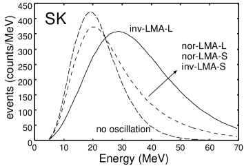
Fig. 3: The time-integrated energy spectra (left) and the time evolution of the number of neutrino events (right) at SK. In these figures, only $\bar{\mathchar 28951\relax}_{e}p$ CC interaction is taken into account.

Fig. 4: The time-integrated energy spectra (left) and the time evolution of the number of neutrino events (right) at SNO. In these figures, only $\mathchar 28951\relax_{e}d$ CC interaction is taken into account.

Fig. 5: The time-integrated energy spectra (left) and the time evolution of the number of neutrino events (right) at SNO. In these figures, only $\bar{\mathchar 28951\relax}_{e}d$ CC interaction is taken into account.

Table I: Number of events at SK

hierarchy	normal		inverted
model	LMA-L	LMA-S	LMA-L	LMA-S	no osc
$\bar{\mathchar 28951\relax_{e}}p$	9459	9427	12269	9441	8036
$\mathchar 28951\relax_{e}e^{-}$	186	171	171	171	132
$\bar{\mathchar 28951\relax_{e}}e^{-}$	46	46	56	46	42
$\mathchar 28951\relax_{\mathchar 28950\relax}e^{-}$	25	26	27	26	30
$\bar{\mathchar 28951\relax_{\mathchar 28950\relax}}e^{-}$	24	23	12	23	24
$\mathchar 28951\relax_{\mathchar 28956\relax}e^{-}$	25	26	26	26	30
$\bar{\mathchar 28951\relax_{\mathchar 28956\relax}}e^{-}$	24	23	12	23	24
$O\mathchar 28951\relax_{e}$	297	214	297	214	31
$O\bar{\mathchar 28951\relax_{e}}$	160	158	296	159	92
total	10245	10114	13084	10129	8441
burst	15.7	16.7	20.1	16.7	12.4

Table II: Number of events (CC) at SNO

hierarchy	normal		inverted
model	LMA-L	LMA-S	LMA-L	LMA-S	no osc
$\mathchar 28951\relax_{e}d{\rm(CC)}$	237	185	185	185	68
$\bar{\mathchar 28951\relax_{e}}d{\rm(CC)}$	118	117	190	117	82
total	355	302	375	302	150
burst	0.6	1.1	1.1	1.1	2.1

3.3 Distinction between Models

In general neutrino oscillation makes the $\mathchar 28951\relax_{e}$ and $\bar{\mathchar 28951\relax}_{e}$ spectra harder, since the original average energies of $\mathchar 28951\relax_{e}$ and $\bar{\mathchar 28951\relax}_{e}$ are smaller than that of $\mathchar 28951\relax_{x}$. In other words neutrino oscillation produces high energy $\mathchar 28951\relax_{e}$ and $\bar{\mathchar 28951\relax}_{e}$ from $\mathchar 28951\relax_{x}$. As a result, the high-energy events increase and the low-energy events decrease. The boundary between high energy and low energy is around 20 MeV. Note that how much these increase and decrease are depends on the adiabaticity parametes, and then the neutrino oscillation parameters, as can be seen in Fig. 3, 4 and 5. This feature can be used as a criterion of the magnitude of the neutrino oscillation effects. We define the following ratios of high-energy to low-energy events at both detectors:

$$R_{\rm SK}\equiv\frac{\makebox{number of events at }20<E<70\rm{MeV}}{\makebox{number of events at }5<E<20\rm{MeV}},$$ (3.5)

$$R_{\rm SNO}\equiv\frac{\makebox{number of events at }20<E<70\rm{MeV}}{\makebox{number of events at }5<E<20\rm{MeV}}.$$ (3.6)

Note that the energy range for the definitions of $R_{\rm SK}$ and $R_{\rm SNO}$ are different from those in the previous paper [27]. The plots of $R_{\rm SK}$ vs $R_{\rm SNO}$ are shown in Fig. 6. In the left figure, we consider only $\mathchar 28951\relax_{e}d$ CC events at SNO for $R_{\rm SNO}$ assuming $\mathchar 28951\relax_{e}d$ CC event and $\bar{\mathchar 28951\relax}_{e}d$ CC event can be distinguished completely. On the other hand, in the right figure we assume that $\mathchar 28951\relax_{e}d$ CC event and $\bar{\mathchar 28951\relax}_{e}d$ CC event can not be distinguished at all and we sum $\mathchar 28951\relax_{e}d$ CC events and $\bar{\mathchar 28951\relax}_{e}d$ CC events for $R_{\rm SNO}$. The error bars represent the statistical errors.

Fig. 6: Plots of $R_{\rm SK}$ vs $R_{\rm SNO}$. In the left figure, only $\mathchar 28951\relax_{e}d$ CC events at SNO are considered for $R_{\rm SNO}$. In the right figure we sum $\mathchar 28951\relax_{e}d$ CC events and $\bar{\mathchar 28951\relax}_{e}d$ CC events to calculate $R_{\rm SNO}$. The errorbars show statistical errors only.

Note that $\mathchar 28951\relax_{e}$ flux and $\bar{\mathchar 28951\relax}_{e}$ flux have essentially different information about the neutrino oscillation parameters. For example, inverted-LMA-L and inverted-LMA-S are distinguishable from $\bar{\mathchar 28951\relax}_{e}$ events but are not from $\mathchar 28951\relax_{e}$ events. So it is more effective to distinguish between models if $\mathchar 28951\relax_{e}d$ CC events and $\bar{\mathchar 28951\relax}_{e}d$ CC events at SNO can be distinguished perfectly. This can be clearly seen in Fig. 6. In the left figure it is easier to distinguish between normal-LMA-L and (normal-LMA-S and inverted-LMA-S) than in the right figure. But even in the left figure, it may be difficult to distinguish between normal-LMA-L and (normal-LMA-S and inverted-LMA-S) considering some ambiguities discussed in the following sections.

3.4 Uncertainties in the original spectra

One of the crucial ingredients in this study is the flavor-dependences of the original spectra. Smaller differences will make it more difficult to distinguish between various models. There have been many numerical simulations of core collapse but the predicted luminosities and temperatures of neutrinos are different from group by group. Numerical model by the Livermore group[36], adopted in this paper, has the great advantage that it covers the full evolution of supernova: from the core collapse over the explosion to the cooling phase of the protoneutron star, although it involves rather traditional treatments of neutrinos.

There are simulations with more sophisticated treatments of neutrinos but they do not obtain explosions and neutrino fluxes for only less than 1 sec are available now[41, 42]. These simulations predict less average-energy differences between flavors compared to those of the Livermore group: $E_{x}/E_{e}\sim 1.4$ [41], 1.7[42], $E_{x}/E_{\bar{e}}\sim 1.1$ [41], 1.3[42], where $E_{e},E_{\bar{e}}$ and $E_{x}$ are the average energies of $\mathchar 28951\relax_{e},\bar{\mathchar 28951\relax}_{e}$ and $\mathchar 28951\relax_{x}$, respectively. To see the effect of the uncertainties in the temperature differences on our analysis, we perform similar analyses varying $\mathchar 28951\relax_{x}$ temperature as stated below and fixing $\mathchar 28951\relax_{e}$ and $\bar{\mathchar 28951\relax}_{e}$ temperatures. This is relevant because various simulations agree well with respect to $\mathchar 28951\relax_{e}$ and $\bar{\mathchar 28951\relax}_{e}$ temperatures. The original spectra can be fitted by the “pinched” Fermi-Dirac distribution,

$$f(E,T_{\mathchar 28939\relax},\mathchar 28945\relax_{\mathchar 28939\relax})\propto\frac{E^{2}}{e^{E/T_{\mathchar 28939\relax}-\mathchar 28945\relax_{\mathchar 28939\relax}}+1},$$ (3.7)

where the temperature $T_{\mathchar 28939\relax}$ and the pinching parameter $\mathchar 28945\relax_{\mathchar 28939\relax}$ for each flavor ($\mathchar 28939\relax=e,\bar{e}$ and $x$) are

$$(T_{\mathchar 28939\relax},\mathchar 28945\relax_{\mathchar 28939\relax}) = (2.8{\rm MeV},2.6)\;\;{\rm for}\;\mathchar 28951\relax_{e},$$ (3.8)

$$(4.0{\rm MeV},2.5)\;\;{\rm for}\;\bar{\mathchar 28951\relax}_{e},$$

$$(7.0{\rm MeV},0)\;\;{\rm for}\;\mathchar 28951\relax_{x}.$$

We consider the following transformation of the distribution function of $\mathchar 28951\relax_{x}$ which has temperature $T_{x}$,

$$f(E,T_{x},\mathchar 28945\relax_{x})\rightarrow\left(\frac{T_{x}}{T^{\prime}_{x}}\right)^{2}f(E\frac{T^{\prime}_{x}}{T_{x}},T^{\prime}_{x},\mathchar 28945\relax_{x})$$ (3.9)

and we regard it as the distribution function of $\mathchar 28951\relax_{x}$ which has temperature $T^{\prime}_{x}$. Note that this transformation conserves the total energy of $\mathchar 28951\relax_{x}$. Based on this spectrum with various values of $T_{x}$, we obtain $R_{\rm SK}$ and $R_{\rm SNO}$ in the same way as in the previous subsections. Fig. 7 shows $T_{x}/T_{e}$ and $T_{x}/T_{\bar{e}}$ dependencies of $R_{\rm SNO}$ and $R_{\rm SK}$, respectively. In the left figure, only $\mathchar 28951\relax_{e}$ events are considered to calculate $R_{\rm SNO}$. Predicted values by the Livermore group simulations are $T_{x}/T_{e}=1.9$ and $T_{x}/T_{\bar{e}}=1.4$, respectively. It should be noted that $T_{x}/T_{e}$ and $T_{x}/T_{\bar{e}}$ are not independent parameters here since we fix $T_{e}$ and $T_{\bar{e}}$.

As can be seen, smaller values of these ratios result in smaller separation of event ratio between different models. In the left figure the errorbars overlap each other if the temperature ratio is less than 1.5. On the other hand, it seems that inverted-LMA-L and the others can be discriminated independent of the temperature ratio. The reason why $R_{\rm SK}$ is significantly different between inverted-LMA-L and the others is that the pinching parameter is different between $\mathchar 28951\relax_{e}$ and $\mathchar 28951\relax_{x}$. By the same reason, $R_{\rm SNO}$ for normal-LMA-L is not the same those for the others even if $T_{x}/T_{e}=1$. Although the relevance of the transformation (3.9) is difficult to argue when $T_{x}/T_{\bar{e}}$ is nearly unity, the possibility of the discrimination between inverted-LMA-L and the others will be robust against the change of $\mathchar 28951\relax_{x}$ temperature of about $10\%$.

Fig. 7: Temperature ratio dependence of the event ratio at SNO and SK. $T_{x}/T_{e}$ vs $R_{\rm SNO}$ in the left and $T_{x}/T_{\bar{e}}$ vs $R_{\rm SK}$ in the right. In the left figure, only $\mathchar 28951\relax_{e}$ events are considered. The errorbars show statistical errors only.

3.5 Dependence on $\mathchar 28946\relax_{13}$

So far we have considered only two extreme cases: H-resonance is perfectly adiabatic and nonadiabatic. It is interesting to investigate the intermediate cases. In Fig. 8 we show $\mathchar 28946\relax_{13}$ dependence of $R_{\rm SK}$ and $R_{\rm SNO}$. Only $\mathchar 28951\relax_{e}$ events are taken into account to calculate $R_{\rm SNO}$. Note that $R_{\rm SK}$ and $R_{\rm SNO}$ vary only in the case of inverted and normal hierarchy, respectively, as will be expected from Fig. 6. In the case of normal hierarchy it will be difficult to determine the value of $\mathchar 28946\relax_{13}$ due to large statistical errors but will be possible to say whether it is very large or very small. On the other hand, in the case of inverted hierarchy the overlap of the errorbars are small even in the intermediate cases. If $\mathchar 28946\relax_{13}$ is rather large ($\sin^{2}{2\mathchar 28946\relax_{13}}>10^{-3}$) the mass hierarchy will be identified.

Fig. 8: $\mathchar 28946\relax_{13}$ dependence of $R_{\rm SK}$ and $R_{\rm SNO}$. Only $\mathchar 28951\relax_{e}$ events are taken into account to calculate $R_{\rm SNO}$. The errorbars show statistical errors only.

3.6 Earth Effects

Depending on the detector position, neutrino go through the Earth and the matter effect inside the Earth can change the neutrino spectra again. For the matter density of the Earth, neutrino oscillation between only two light neutrinos is involved. Since the oscillation length in the Earth, which depends on the neutrino energy, is the same order as the Earth radius for the neutrino parameter adapted here, the Earth matter effect appear as a distosion in the spectra [29, 30, 31, 32, 33].

The numerical process to calculate the Earth effect is the same as described above except that the density profile of the Earth is needed. We use a realistic density profile [43]. In Fig. 9 neutrino spectra in the case that the nadir angle is $30^{\circ}$ and $70^{\circ}$ are shown with that in absence of the Earth effects. The left figure is the $\mathchar 28951\relax_{e}$ spectra at SNO and the right figure is the $\bar{\mathchar 28951\relax}_{e}$ spectra at SK. The Earth effect is absent in $\mathchar 28951\relax_{e}$ and $\bar{\mathchar 28951\relax}_{e}$ in case of normal-LMA-L and inverted-LMA-L, respectively. This is because in these cases H-resonance is perfectly adiabatic and low-energy neutrinos, which were originally $\mathchar 28951\relax_{e}$ in the supernova core, are converted to the heaviest neutrino, which is not involved in the matter oscillation in the Earth. Thus the detection of the Earth effect will be helpful to distinguish models, especially normal-LMA-L from normal-LMA-S and inverted-LMA-S.

The form of the distorted spectra depends on the nadir angle of the neutrino path. The nadir angle $30^{\circ}$ and $70^{\circ}$ correspond to one of the path with which neutrino pass through core and mantle, and only mantle, respectively. The detectability of the Earth effect was discussed by us [30] and it is shown that complementary observation by SK, SNO and Large Volume Detector (LVD) is effective for its detection.

Fig. 9: Distorted spectra due to the Earth effects. The left figure is the $\mathchar 28951\relax_{e}$ spectra at SNO and the right figure is the $\bar{\mathchar 28951\relax}_{e}$ spectra at SK. Neutrino spectra in the case that the nadir angle is $30^{\circ}$ and $70^{\circ}$ are shown with that in absence of the Earth effects.

4 Discussion and Conclusion

There are some ambiguities besides those descussed above. The first is the direction of the supernova. If the supernova can be observed optically, the direction can be known with enough accuracy. But if the supernova is at the Galactic Center, it might be hidden by the large amount of gas and could not be seen optically. Pointing by the electron scattering events of the supernova neutrino is studied by several authors [44, 45] and the accuracy is expected to be $\sim 7^{\circ}$. More detailed analyses of the Earth effects have been studied considering the locations of the detectors and the direction of the supernova [30, 32].

Another is the mass of the progenitor star. It affects the mass of the iron core, which affects the neutrino spectra [42, 46, 47]. Study including the mass uncertainty is now in progress but the preliminary result is that the mass uncertainty is not important in our analysis [48].

Recently effects of shock propagation on neutrino oscillation in supernova have been studied [49, 50, 24, 51] and it was shown that some characteristic signatures may emerge as the shock propagates through the regions where matter-enhanced neutrino flavor conversion occurs. As we show [50], shock propagation effect will be safely removed by taking only early-phase events into account.

We studied the effects of neutrino oscillation on supernova neutrino in the case of the inverted mass hierarchy as well as the normal mass hierarchy. Numerical analysis using a realistic supernova and presupernova model allowed us to discuss quantitatively a possibility to probe neutrino oscillation parameters. We showed that degeneracy exists only between normal-LMA-S and inverted-LMA-S if the Earth effect is taken into account and that $\mathchar 28946\relax_{13}$ can be well probed by SK if the neutrino mass hierarchy is inverted case. Errors due to the uncertainty of the original neutrino spectra are also estimated.

5 Acknowledgments

K.T.’s work is supported by Grant-in-Aid for JSPS Fellows. K.S.’s work is supported by Grant-in-Aid for Scientific Research (S) No. 14102004 and Grant-in-Aid for Scientific Research on Priority Areas No. 14079202.

References

- [1] Y. Fukuda et al., Phys. Rev. Lett. 82 (1999) 2644.
- [2] S. Fukuda et al., Phys. Rev. Lett. 86 (2001) 5656.
- [3] SNO Collaboration, Phys. Rev. Lett. 87 (2001) 071301.
- [4] J. N. Bahcall, M. C. Gonzalez-Garcia and C. Pena-Garay, JHEP 0207 (2002) 054.
- [5] V. Barger, D. Marfatia, K. Whisnant and B. P. Wood, Phys. Lett. B 537 (2002) 179.
- [6] P. C. de Holanda and A. Yu. Smirnov, hep-ph/0205241.
- [7] KamLAND Collaboration, K. Eguchi et al., Phys. Rev. Lett. 90 (2003) 021802.
- [8] M. Apollonio et al., Phys. Lett. B 466 (1999) 415.
- [9] H. Minakata and H. Sugiyama, Phys. Lett. B 526 (2002) 335.
- [10] G. G. Raffelt, Nucl. Phys. Proc. Suppl. 110 (2002) 254.
- [11] F. Cei, Int. J. Mod. Phys. A 17 (2002) 1765.
- [12] G. G. Raffelt, astro-ph/0302589.
- [13] S. M. Bilenky, C. Giunti, J. A. Grifols and E. Massó, hep-ph/0211462.
- [14] K. Hirata et al., Phys. Rev. Lett. 58, 1490 (1987).
- [15] R. M. Bionta et al., Phys. Rev. Lett. 58, 1494 (1987).
- [16] J. Arafune and M. Fukugita, Phys. Rev. Lett. 59, 367 (1987).
- [17] K. Sato and H. Suzuki, Phys. Rev. Lett. 58, 2722 (1987).
- [18] I. Goldman et al., Phys. Rev. Lett. 60, 1789 (1988).
- [19] B. Jegerlehner, F. Neubig and G. Raffelt, Phys. Rev. D 54 (1996) 1194.
- [20] C. Lunardini and A. Yu. Smirnov, Phys. Rev. D 63 (2001) 073009.
- [21] H. Minakata and H. Nunokawa, Phys. Lett. B 504 301 (2001).
- [22] A. S. Dighe and A. Yu. Smirnov, Phys. Rev. D 62 (2000) 033007.
- [23] G. L. Fogli, E. Lisi, D. Montanino and A. Palazzo, Phys. Rev. D 65 (2002) 073008.
- [24] C. Lunardini and A. Yu. Smirnov, hep-ph/0302033.
- [25] A. S. Dighe, M. Th. Keil and G. G. Raffelt, hep-ph/0303210.
- [26] A. S. Dighe, M. Th. Keil and G. G. Raffelt, hep-ph/0304150.
- [27] K. Takahashi, M. Watanabe, K. Sato and T. Totani, Phys. Rev. D 64 (2001) 093004.
- [28] SNO Collaboration, Phys. Rev. Lett. 89 (2002) 011302.
- [29] K. Takahashi, M. Watanabe and K. Sato, Phys. Lett. B 510 (2001) 189.
- [30] K. Takahashi and K. Sato, Phys. Rev. D 66 (2002) 033006.
- [31] A. S. Dighe, hep-ph/0106325.
- [32] C. Lunardini and A. Yu. Smirnov, Nucl. Phys. B 616 (2001) 307.
- [33] A. S. Dighe, M. T. Keil and G. G. Raffelt, hep-ph/0304150.
- [34] H. Suzuki: Supernova Neutrino in Physics and Astrophysics of Neutrino, edited by M. Fukugita and A. Suzuki (Springer-Verlag, Tokyo, 1994).
- [35] E. Kh. Akhmedov, C. Lunardini and A. Yu. Smirnov, Nucl. Phys. B 643 (2002) 339-366.
- [36] J. R. Wilson, R. Mayle, S. Woosley, T. Weaver, Ann. NY Acad. Sci. 470, 267 (1986).
- [37] T. Totani, K. Sato, H. E. Dalhed and J. R. Wilson, Astrophys. J. 496 (1998) 216.
- [38] A. Friedland, Phys. Rev. D 64 (2001) 013008.
- [39] S. E. Woosley and T. A. Weaver, ApJ. Suppl. 101 (1995) 181.
- [40] J. N. Bahcall, M. C. Gonzalez-Garcia and C. Pena-Garay, JHEP 02 (2003) 009.
- [41] H. -T. Janka, R. Buras, K. Kifonidis, T. Plewa and M. Rampp, in Core Collapse of Massive Stars, edited by C. L. Fryer (Kluwer Academic Publ., Dordrecht, 2003), astro-ph/0212314; G. G. Raffelt, M. Th. Keil, R. Buras, H. -T. Janka and M. Rampp, Proc. NOON 03 (10-14 February 2003, Kanazawa, Japan), astro-ph/0303226; R. Buras, M. Rampp, H. -T. Janka and K. Kifonidis, astro-ph/0303171.
- [42] T. A. Thompson, A. Burrows, P. A. Pinto, astro-ph/0211194.
- [43] A. M. Dziewonski and D. L. Anderson, Phys. Earth. Planet Inter. 25 (1981) 297.
- [44] J. F. Beacom and P. Vogel, Phys.Rev. D 60 (1999) 033007.
- [45] S. Ando and K. Sato, Prog. Theor. Phys. 107 (2002) 957.
- [46] R. Mayle, Ph. D. Thesis, University of California (1987).
- [47] R. Mayle, J. R. Wilson, and D. N. Schramm, Astrophys. J. 318 (1987) 288.
- [48] K. Takahashi, K. Sato, T. A. Thompson and A. Burrows, in progress.
- [49] R. C. Schirato and G. M. Fuller, astro-ph/0205390.
- [50] K. Takahashi, K. Sato, H. E. Dalhed and J. R. Wilson, astro-ph/0212195.
- [51] G. L. Fogli, E. Lisi, A. Mirizzi and D. Montanino, hep-ph/0304056.