UMD-PP-02-048

Neutrino oscillation data versus

minimal supersymmetric SO(10) model

Takeshi Fukuyama

Department of Physics, Ritsumeikan University, Kusatsu, Shiga 525-8577, Japan

Nobuchika Okada

Department of Physics, University of Maryland, College Park, MD 20742, USA

Abstract

We reconsider the minimal supersymmetric SO(10) model, where only one 10 and one $\overline{\bf 126}$ Higgs multiplets have Yukawa couplings with matter multiplets. The model is generalized to include CP-violating phases, and examined how well its predictions can meet the current neutrino oscillation data. Using the electroweak scale data about six quark masses, three angles and one CP-phase in the Cabibbo-Kobayashi-Maskawa matrix and three charged-lepton masses and given $\tan\beta$ (the ratio of vacuum expectation values of a pair of Higgs doublets), we obtain the Pontecorvo-Maki-Nakagawa-Sakata matrix and the ratio, $\Delta m_{\odot}^{2}/\Delta m_{\oplus}^{2}$, as functions of only one free parameter in the model. In our analysis, one-loop renormalization group equations for the gauge couplings, the Yukawa couplings and the effective dimension-five operator are used to connect the data between the electroweak scale and the grand unification scale. Fixing the free parameter appropriately, we find, for example, $\sin^{2}2\theta_{12}\sim 0.72$, $\sin^{2}2\theta_{23}\sim 0.90$, $\sin^{2}2\theta_{13}\sim 0.16$ and $\Delta m_{\odot}^{2}/\Delta m_{\oplus}^{2}\sim 0.19$ with $\tan\beta=45$, which are in agreement with the current neutrino oscillation data.

1 Introduction

Supersymmetry (SUSY) extension is one of the most promising ways to provide a solution to the gauge hierarchy problem in the standard model [1]. The minimal version of this extension is called the minimal supersymmetric standard model (MSSM). Interestingly, the experimental data support the unification of the three gauge couplings at the scale $M_{GUT}\sim 2\times 10^{16}\mbox{GeV}$ with the MSSM particle contents [2]. At high energies, our world may be described by a SUSY grand unified theory (GUT) with a simple gauge group such as SU(5) or SO(10) into which all the gauge groups in the standard model are embedded and unified.

On the other hand, much information about quark and lepton mass matrices has been accumulated in these decades. Especially, there exist, at present, strong evidences of neutrino masses and mixings through the interpretation of the (active) neutrino oscillations as the solutions to the solar neutrino deficit [3, 4, 5, 6, 7, 8] and the atmospheric neutrino anomaly [9]. According to the results, the MSSM has to be extended so as to incorporate neutrino masses and mixings.

In these points of view, the supersymmetric SO(10) GUT model is one of the most well-motivated theories, since the right-handed neutrinos are naturally incorporated and unified into the same multiplet, 16, together with the ordinary matters in the MSSM. Furthermore, this model has an additional advantage that the smallness of the neutrino masses can be naturally explained through the see-saw mechanism [10] with large right-handed Majorana neutrino masses.

There are many possibilities for the Higgs sector that will make the model realistic: namely, it correctly breaks the SO(10) gauge symmetry into the standard model one, reproduces observed fermion masses, mixings and CP-phase, and realizes the doublet-triplet Higgs mass splitting (in terminology of SU(5) GUT) etc. In this paper, we concentrate our discussion on the fermion masses and mixings, and consider the so-called “minimal” SO(10) model where only one 10 and one $\overline{\bf 126}$ Higgs multiplets have Yukawa couplings with quarks and leptons. It is very interesting to investigate this model, since it can fix all the fermion mass matrices including, at present, ambiguous and undetermined ones.

The minimal model was first seriously considered by Babu and Mohapatra [11] (non-SUSY case) and Lee and Mohapatra [12] (SUSY case), where the neutrino oscillation parameters were predicted with inputs of six quark masses, three mixing angles in the Cabibbo-Kobayashi-Maskawa (CKM) matrix and three charged-lepton masses. Unfortunately, the predictions were revealed to contradict the current experimental data. For example, the predicted mixing angle, $\sin^{2}2\theta_{23}$, in the Pontecorvo-Maki-Nakagawa-Sakata (PMNS) matrix was found to be too small to be consistent with the the atmospheric neutrino oscillation data [9]. It seems to be inevitable that the minimal model should be extended by introducing new Higgs multiplets so as to incorporate the realistic neutrino oscillation parameters.

However, note that, in Refs. [11] and [12], only the CP invariant case was analyzed. It was recently pointed out [13] that, once CP-violating phases are taken into account in the minimal model, there exits the parameter region which cannot be excluded by the current neutrino oscillation data. This observation brings a new hope to obtain the minimal SO(10) model compatible with all the observed data of fermion mass matrices. Nevertheless, more elaborate studies are needed, since, in [13], the GUT relation among the charged fermion mass matrices was applied to the mass matrices at the electroweak scale. This treatment is incomplete because the GUT relation is valid only at the GUT scale. In fact, we can see that Yukawa couplings evolve according to the renormalization group equations (RGEs), and the GUT relation is lost after the running in the “long desert” between the GUT scale and the electroweak scale.

In this paper, we pursue this program in more correct and complete way. Our strategy is the following. First, we evaluate the data of charged fermion mass matrices at the GUT scale by extrapolating the data at the electroweak scale according to their Yukawa coupling REGs. Next, these GUT scale data are applied to the GUT relation that is generalized to include CP-violating phases. This leads us to the explicit form of neutrino mass matrix at the GUT scale via the GUT relation. Lastly, running it back to the electroweak scale according to the RGE for the effective dimension-five operator [14], we compare our result with the current neutrino oscillation data.

This paper is organized as follows: in the next section, we give our basic framework of the minimal SUSY SO(10) model with one 10 and one $\overline{\bf 126}$ Higgs multiplets, and discuss the GUT relation among the fermion mass matrices. In Sec. 3, RGEs we use in our analysis are introduced. In Sec. 4, numerical analysis is performed, and the results are presented. Other predictions from our resultant mass matrices are discussed in Sec. 5. The last section is devoted to summary and comments.

2 Minimal SO(10) model and fermion mass matrices

We consider the minimal SUSY SO(10) model with a pair of 10+$\overline{\bf 126}$ Higgs multiplets, only which have Yukawa couplings (superpotential) with the matter multiplets such as

$$W_{Y}=Y_{10}^{ij}{\bf 16}_{i}H_{10}{\bf 16}_{j}+Y_{126}^{ij}{\bf 16}_{i}H_{126}{\bf 16}_{j}\;,$$ (1)

where ${\bf 16}_{i}$ is the matter multiplet of the i-th generation, $H_{10}$ and $H_{126}$ are the Higgs multiplet of 10 and $\overline{\bf 126}$ representations under SO(10), respectively. Note that, by virtue of the gauge symmetry, the Yukawa couplings, $Y_{10}$ and $Y_{126}$, are complex symmetric $3\times 3$ matrices. In our model, these Yukawa couplings are assumed to be real as in the original model [11] to keep the number of free parameters minimum.

In the SUSY GUT scenario, the GUT gauge symmetry is broken at the GUT scale, $M_{GUT}\sim 10^{16}$ GeV, into the standard model one. There are some different breaking chains suitable for our aim. Here, suppose the intermediate pass through the Pati-Salam subgroup [15], $G_{422}=SU(4)_{c}\times SU(2)_{L}\times SU(2)_{R}$, for simplicity. Under this gauge symmetry, the above Higgs multiplets are decomposed as ${\bf 10}\rightarrow({\bf 6},{\bf 1},{\bf 1})+({\bf 1},{\bf 2},{\bf 2})$ and $\overline{\bf 126}\rightarrow({\bf 6},{\bf 1},{\bf 1})+({\bf 10},{\bf 3},{\bf 1})+(\overline{\bf 10},{\bf 1},{\bf 3})+({\bf 15},{\bf 2},{\bf 2})$, while ${\bf 16}\rightarrow({\bf 4},{\bf 2},{\bf 1})+(\overline{\bf 4},{\bf 1},{\bf 2})$ for the matter multiplet. Breaking down to the standard model gauge group, $SU(4)_{c}\times SU(2)_{R}\rightarrow SU(3)_{c}\times U(1)_{Y}$, is accomplished by vacuum expectation value (VEV) of the $(\overline{\bf 10},{\bf 1},{\bf 3})$ Higgs multiplet. Note that the Majorana masses for the right-handed neutrinos are also generated by this VEV through the Yukawa coupling $Y_{126}$ in Eq. (1).

After this symmetry breaking, we find two pair of Higgs doublets which are in the same representation as the pair in the MSSM. One pair comes from $({\bf 1},{\bf 2},{\bf 2})\subset{\bf 10}$ and the other comes from $(\overline{\bf 15},{\bf 2},{\bf 2})\subset\overline{\bf 126}$. Using these two pairs of the Higgs doublets, the Yukawa couplings of Eq. (1) are rewritten as

$$W_{Y} = \overline{u}_{i}\left(Y_{10}^{ij}H^{u}_{10}+Y_{126}^{ij}H^{u}_{126}\right)q_{j}+\overline{d}_{i}\left(Y_{10}^{ij}H^{d}_{10}+Y_{126}^{ij}H^{d}_{126}\right)q_{j}$$ (2)

$$+ \overline{\nu}_{i}\left(Y_{10}^{ij}H^{u}_{10}-3Y_{126}^{ij}H^{u}_{126}\right)\ell_{j}+\overline{e}_{i}\left(Y_{10}^{ij}H^{d}_{10}-3Y_{126}^{ij}H^{d}_{126}\right)\ell_{j}$$

$$+ \overline{\nu}_{i}\left(Y_{126}^{ij}\;v_{R}\right)\overline{\nu}_{j}\;,$$

where $\overline{u}$, $\overline{d}$, $\overline{\nu}$ and $\overline{e}$ are the right-handed $SU(2)_{L}$ singlet quark and lepton superfields, $q$ and $\ell$ are the left-handed $SU(2)_{L}$ doublet quark and lepton superfields, $H_{10}^{u,d}$ and $H_{126}^{u,d}$ are up-type and down-type Higgs doublet superfields originated from $H_{10}$ and $H_{126}$, respectively, and the last term is the Majorana mass term of the right-handed neutrinos with VEV of the $(\overline{\bf 10},{\bf 1},{\bf 3})$ Higgs, $v_{R}$. Quarks and leptons acquire Dirac masses through VEVs of these Higgs doublets. Note that, in that case, the entry of the Clebsch-Gordan coefficient, $-3$, in the lepton sector plays the crucial role so that the unwanted GUT relations, $m_{d}=m_{e}$ and $m_{s}=m_{\mu}$, are corrected [11] in the same manner discussed by Georgi and Jarlskog [16].

Here, remember that the gauge coupling unification succeeds with only the MSSM particle contents. This means that only one pair of Higgs doublets remains light and the others should be heavy ($\geq M_{G}$). It is highly non-trivial to accomplish this task naturally, while keeping the crucial role of $H_{126}^{u,d}$ to the fermion masses. This problem is essentially the same problem as the doublet-triplet Higgs mass splitting problem, and is referred as the “doublet-doublet splitting problem”. In this paper, we assume that this splitting is realized.

Now let us see the low energy superpotential of our model. After realizing the doublet-doublet Higgs mass splitting, we obtain only one pair of light Higgs doublets ($H_{u}$ and $H_{d}$) in the MSSM, which are, in general, admixture of all Higgs doublets having the same quantum numbers in the original model such as

$$H_{u} = \tilde{\alpha}_{u}H_{10}^{u}+\tilde{\beta}_{u}H_{126}^{u}+\cdots$$

$$H_{d} = \tilde{\alpha}_{d}H_{10}^{d}+\tilde{\beta}_{d}H_{126}^{d}+\cdots\;,$$ (3)

where “$+\cdots$” denotes the mixing with other Higgs doublets in the model (about which we do not discuss), $\tilde{\alpha}_{u,d}$ and $\tilde{\beta}_{u,d}$ denote elements of the unitary matrix which rotate the flavor basis in the original model into the (SUSY) mass eigenstates. Omitting the heavy Higgs mass eigenstates, the low energy superpotential is described by only the light Higgs doublets $H_{u}$ and $H_{d}$ such that

$$W_{Y} = \overline{u}_{i}\left(\alpha^{u}Y_{10}^{ij}+\beta^{u}Y_{126}^{ij}\right)H_{u}q_{j}+\overline{d}_{i}\left(\alpha^{d}Y_{10}^{ij}+\beta^{d}Y_{126}^{ij}\right)H_{d}q_{j}$$ (4)

$$+ \overline{\nu}_{i}\left(\alpha^{u}Y_{10}^{ij}-3\beta^{u}Y_{126}^{ij}\right)H_{u}\ell_{j}+\overline{e}_{i}\left(\alpha^{d}Y_{10}^{ij}-3\beta^{d}Y_{126}^{ij}\right)H_{d}\ell_{j}$$

$$+ \overline{\nu}_{i}\left(Y_{126}^{ij}v_{R}\right)\overline{\nu}_{j}\;,$$

where the formulas of the inverse unitary transformation of Eq. (3), $H_{10}^{u,d}=\alpha^{u,d}H_{u,d}+\cdots$ and $H_{126}^{u,d}=\beta^{u,d}H_{u,d}+\cdots$, have been used. Note that the elements of the unitary matrix, $\alpha^{u,d}$ and $\beta^{u,d}$, are in general complex parameters, through which CP-violating phases are introduced into the fermion mass matrices.

Providing the Higgs VEVs, $H_{u}=v\sin\beta$ and $H_{d}=v\cos\beta$ with $v=174\mbox{GeV}$, the quark and lepton mass matrices can be read off as

$$M_{u} = c_{10}M_{10}+c_{126}M_{126}$$

$$M_{d} = M_{10}+M_{126}$$

$$M_{D} = c_{10}M_{10}-3c_{126}M_{126}$$

$$M_{e} = M_{10}-3M_{126}$$

$$M_{R} = c_{R}M_{126}\;,$$ (5)

where the mass matrices are defined as $M_{10}=Y_{10}\alpha^{d}v\cos\beta$ and $M_{126}=Y_{126}\beta^{d}v\cos\beta$, respectively, $c_{10}=(\alpha^{u}/\alpha^{d})\tan\beta$, $c_{126}=(\beta^{u}/\beta^{d})\tan\beta$, and $c_{R}=v_{R}/(\beta^{d}v\cos\beta)$. All the quark and lepton mass matrices are characterized by only two basic mass matrices, $M_{10}$ and $M_{126}$, and three coefficients. This means the strong predictability of the model to the fermion mass matrices in the MSSM.

Now let us count how many free parameters are included in the above mass matrices, not counting $c_{R}$. Remember that we began with real symmetric matrices $Y_{10}$ and $Y_{126}$. By flavor rotation of the GUT matter multiplets, we can begin with the basis where $M_{10}$ is real and diagonal, which includes three free parameters. There are seven parameters in $M_{126}$: six parameters originate from the symmetric real matrix $Y_{126}$, and one from the phase of $\beta^{d}$. Adding the four parameters from complex $c_{10}$ and $c_{126}$, we find 14 free parameters in total, which are evaluated as six quark masses, three angles and one CP-phase in the CKM matrix and three charged-lepton masses, but one parameter is left free [17]. Now two free parameters are newly introduced in addition to 12 free parameters analyzed in [11] and [12], by which our model is generalized to include CP-violating phases.

The parameter, $c_{R}$, appears in the right-handed Majorana neutrino mass matrix, by which masses of the right-handed Majorana neutrinos are determined after $M_{126}$ are fixed. Since $v_{R}\sim M_{G}$, $c_{R}\sim v_{R}/v\sim 10^{14}\mbox{GeV}$ is naturally expected. However, we treat $c_{R}$ as a free parameter in the following analysis, since the Higgs multiplet breaking $G_{422}$, in general, mixes with other Higgs multiplets being in the same representation under $G_{422}$. Also there should exist Higgs multiplets which also have $G_{422}$ breaking VEV to cancel the D-term VEV and ensure SUSY. In addition, threshold corrections would introduce an uncertainty of $v_{R}$.

The mass matrix formulas in Eq.(5) leads to the GUT relation among the quark and lepton mass matrices,

$$M_{e}=c_{d}\left(M_{d}+\kappa M_{u}\right)\;,$$ (6)

where

$$c_{d} = -\frac{3c_{10}+c_{126}}{c_{10}-c_{126}}$$

$$\kappa = -\frac{4}{3c_{10}+c_{126}}\;.$$ (7)

Without loss of generality, we can begin with the basis where $M_{u}$ is real and diagonal, $M_{u}=D_{u}$. Since $M_{d}$ is the symmetric matrix, it can be described as $M_{d}=V_{KM}^{*}D_{d}V_{KM}^{\dagger}$ by using the CKM matrix $V_{KM}$ and the real diagonal mass matrix $D_{d}$. Considering the basis-independent quantities, $\mbox{tr}[M_{e}^{\dagger}M_{e}]$, $\mbox{tr}[(M_{e}^{\dagger}M_{e})^{2}]$ and $\mbox{det}[M_{e}^{\dagger}M_{e}]$, and eliminating $|c_{d}|$, we obtain two independent equations such that

$$\left(\frac{\mbox{tr}[\tilde{M_{e}}^{\dagger}\tilde{M_{e}}]}{m_{e}^{2}+m_{\mu}^{2}+m_{\tau}^{2}}\right)^{2} = \frac{\mbox{tr}[(\tilde{M_{e}}^{\dagger}\tilde{M_{e}})^{2}]}{m_{e}^{4}+m_{\mu}^{4}+m_{\tau}^{2}}\;,$$ (8)

$$\left(\frac{\mbox{tr}[\tilde{M_{e}}^{\dagger}\tilde{M_{e}}]}{m_{e}^{2}+m_{\mu}^{2}+m_{\tau}^{2}}\right)^{3} = \frac{\mbox{det}[\tilde{M_{e}}^{\dagger}\tilde{M_{e}}]}{m_{e}^{2}\;m_{\mu}^{2}\;m_{\tau}^{2}}\;,$$ (9)

where $\tilde{M_{e}}=V_{KM}^{*}D_{d}V_{KM}^{\dagger}+\kappa D_{u}$. With the input data of six quark masses, three angles and one CP-phase in the CKM matrix and three charged-lepton masses, we can determine $\kappa$ and $|c_{d}|$, but one parameter, the phase of $c_{d}$, is left undetermined [17]. Now the mass matrices, $M_{10}$ and $M_{126}$, are described by

$$M_{10} = \frac{3+|c_{d}|e^{i\sigma}}{4}V_{KM}^{*}D_{d}V_{KM}^{\dagger}+\frac{|c_{d}|e^{i\sigma}\kappa}{4}D_{u}\;,$$ (10)

$$M_{126} = \frac{1-|c_{d}|e^{i\sigma}}{4}V_{KM}^{*}D_{d}V_{KM}^{\dagger}-\frac{|c_{d}|e^{i\sigma}\kappa}{4}D_{u}\;,$$ (11)

as the functions of $\sigma$, the phase of $c_{d}$, with the solutions, $|c_{d}|$ and $\kappa$, determined by the GUT relation.

Note that the GUT relation of Eq. (6) is valid only at the GUT scale. Therefore, the input data needed to determine $\kappa$ and $|c_{d}|$ should be the data at the GUT scale. To evaluate the GUT scale data, RGE analysis of Yukawa couplings is necessary. This is the subject of the next section.

3 One-loop RGEs

The data we need at the GUT scale are six quark masses, three angles and one CP-phase in the CKM matrix and three charged-lepton masses. In general, it is not a straightforward task to obtain the data at GUT scale by extrapolating the data at the electroweak scale. This is because RGEs of quark and charged-lepton Yukawa couplings include unknown neutrino Yukawa couplings. We can obtain a reliable answer only if neutrino Yukawa couplings are negligible.

Fortunately, in models with the see-saw mechanism, the right-handed neutrinos are decoupled at the scale below the heavy Majorana masses, and the neutrino Yukawa couplings become irrelevant and disappear from RGEs of quark and charged-lepton Yukawa couplings. This fact makes our analysis straightforward, at least, below the heavy Majorana mass scale. In the following analysis, we use the RGEs independent of the neutrino Yukawa couplings at all scales between the electroweak and the GUT scales. Although this treatment fails at the scale above the right-handed Majorana neutrino masses, we expect that our results are reliable, since the heavy Majorana mass scale is close to the GUT scale. We will give a comment on this point in the last section.

We analyze one-loop RGEs for gauge couplings and quark and charged-lepton Yukawa couplings in the MSSM. For simplicity, the universal soft SUSY breaking masses are assumed, $m_{SUSY}=M_{Z}\sim 91\mbox{GeV}$. In this case, the GUT scale is found to be $M_{G}\sim 2\times 10^{16}\mbox{GeV}$. The RGEs used in our analysis are as follows [18]. For gauge couplings,

$$\frac{dg_{i}}{d(\ln\mu)}=-\frac{b_{i}}{16\pi^{2}}g_{i}^{3}\;,$$ (12)

where $b_{i}=(3,-1,-33/5)$ for $i=3,2,1$ corresponding to $SU(3)_{c}$, $SU_{L}$ and $U(1)_{Y}$ gauge couplings, respectively. We use the electroweak scale inputs such that $\alpha_{3}(M_{Z})=g_{3}^{2}/4\pi=0.118$, $\alpha_{2}(M_{Z})=g_{3}^{2}/4\pi=0.0335$ and $\alpha_{1}(M_{Z})=g_{3}^{2}/4\pi=0.0168$. On the other hand, RGEs for the Yukawa couplings of up-type quarks ($Y_{u}$), down-type quarks ($Y_{d}$), and charged-leptons ($Y_{e}$) are found to be

$$\frac{dS_{F}}{d(\ln\mu)}=\frac{1}{16\pi^{2}}\left(\beta_{F}S_{F}+S_{F}\beta_{F}\right)\;,$$ (13)

where $S_{F}=Y_{F}^{\dagger}Y_{F}$ with fermion index $F=u,d,e$, and

$$\beta_{u} = 3S_{u}+S_{d}+\left\{\mbox{tr}\left[3S_{u}\right]-\left(\frac{16}{3}g_{3}^{2}+3g_{2}^{2}+\frac{13}{15}g_{1}^{2}\right)\right\}{\bf 1}_{3\times 3}$$

$$\beta_{d} = 3S_{d}+S_{u}+\left\{\mbox{tr}\left[3S_{d}+S_{e}\right]-\left(\frac{16}{3}g_{3}^{2}+3g_{2}^{2}+\frac{7}{15}g_{1}^{2}\right)\right\}{\bf 1}_{3\times 3}$$

$$\beta_{e} = 3S_{e}+\left\{\mbox{tr}\left[3S_{d}+S_{e}\right]-\left(3g_{2}^{2}+\frac{9}{5}g_{1}^{2}\right)\right\}{\bf 1}_{3\times 3}\;.$$ (14)

To determine the input values of fermion Yukawa couplings at $M_{Z}$, we have to fix $\tan\beta$ by hand. For given $\tan\beta$, they are given by

$$S_{u} = \mbox{diag}\left(\frac{m_{u}^{2}}{v^{2}},\frac{m_{c}^{2}}{v^{2}},\frac{m_{t}^{2}}{v^{2}}\right)\left(1+\tan^{-2}\beta\right)\;,$$ (15)

$$S_{d} = V_{KM}\;\mbox{diag}\left(\frac{m_{d}^{2}}{v^{2}},\frac{m_{s}^{2}}{v^{2}},\frac{m_{b}^{2}}{v^{2}}\right)V_{KM}^{\dagger}\left(1+\tan^{2}\beta\right)\;,$$ (16)

$$S_{e} = \mbox{diag}\left(\frac{m_{e}^{2}}{v^{2}},\frac{m_{\mu}^{2}}{v^{2}},\frac{m_{\tau}^{2}}{v^{2}}\right)\left(1+\tan^{-1}\beta\right)\;.$$ (17)

Here, we have worked out in the basis where $S_{u}$ and $S_{e}$ are diagonal. Given $\tan\beta$, it is easy to solve the above RGEs numerically. Although, as can be seen from the above RGEs, $S_{u}$ is no longer diagonal after running, we can extract the data we need at the GUT scale by the usual manner. For example, the CKM matrix at the GUT scale is given by $V_{KM}=V_{u}^{\dagger}V_{d}$, where $V_{u}$ and $V_{d}$ are the unitary matrices which diagonalize $S_{u}$ and $S_{d}$, respectively.

Solving the GUT relation as discussed in the previous section by using the extrapolated data, we can obtain the light Majorana neutrino mass matrix, $M_{\nu}$, as a function of $\sigma$ and $c_{R}$ through Eqs. (5), (10) and (11) and the see-saw mechanism, $M_{\nu}=-M_{D}^{T}M_{R}^{-1}M_{D}$. Since this is the mass matrix at the GUT scale, it should be extrapolated to the electroweak scale according to the RGE for the effective dimension-five operator [14] such that

$$\frac{dM_{\nu}}{d(\ln\mu)}=\frac{1}{16\pi^{2}}\left\{S_{e}^{T}M_{\nu}+M_{\nu}S_{e}+\left(6\mbox{tr}\left[S_{u}\right]-6g_{2}^{2}-\frac{6}{5}g_{1}^{2}\right)M_{\nu}\right\}\;.$$ (18)

After the running, our resultant neutrino mass matrix are compared with the neutrino oscillation data. In the next section, the effect of the RGE running will be found to be small and almost negligible in our model.

4 Numerical analysis and results

Now we are ready to perform all the numerical analysis. Fist of all, note that the solution of the GUT relation exists, only if we take appropriate input parameters. This is because the number of our free parameters (fourteen) are almost the same as the number of inputs (thirteen). Therefore, in the following analysis, we vary two input parameters, $m_{s}$ and CP-phase $\delta$ in the CKM matrix, within the experimental errors so as to find the solution. We take input fermion masses at $M_{Z}$ as follows (in GeV):

$$m_{u}=0.00233\;,\;\;m_{c}=0.677\;,\;\;m_{t}=176$$

$$m_{d}=0.00469\;,\;\;m_{b}=3.00$$

$$m_{e}=0.000487\;,\;\;m_{\mu}=0.103\;,\;\;m_{\tau}=1.75$$

Here, the experimental values extrapolated from low energies to $M_{Z}$ were used [19]. For the CKM mixing angles in the “standard” parameterization, we input the center values measured by experiments as follows [20]:

$$s_{12}=\frac{0.219+0.226}{2},\;\;s_{23}=\frac{0.037+0.043}{2},\;\;s_{13}=\frac{0.002+0.005}{2}\;.$$

Since it is very difficult to search all the possible parameter region systematically, we present only reasonable results we found. In the following, we show our analysis in detail in the case $\tan\beta=45$. Here we take $m_{s}=0.0729\mbox{(GeV)}$ and $\delta=86.4^{\circ}$. In this case, the CKM matrix at $M_{Z}$ is given by

$$V_{KM}(M_{Z})=\left(\begin{array}[]{ccc}0.975&0.222&0.000220-0.00349i\\ -0.222-0.000136i&0.974-0.0000311i&0.0400\\ 0.00869-0.00340i&-0.0390-0.000777i&0.999\end{array}\right)\;.$$ (22)

After RGE evolutions to the GUT scale, fermion masses (up to sign) and the CKM matrix are found as follows (in GeV) :

$$m_{u}=0.00103\;,\;\;m_{c}=0.301\;,\;\;m_{t}=134$$

$$m_{d}=0.00171\;,\;\;m_{s}=0.0265\;,\;\;m_{b}=1.56$$

$$m_{e}=0.000413\;,\;\;m_{\mu}=0.0872\;,\;\;m_{\tau}=1.69$$

and

$$V_{KM}(M_{G})=\left(\begin{array}[]{ccc}0.975&0.222&0.000175-0.00279i\\ -0.222-0.000121i&0.974+0.000129i&0.0320\\ 0.00695-0.00272i&-0.0312-0.000626i&0.999\end{array}\right)\;$$ (26)

in the standard parameterization.

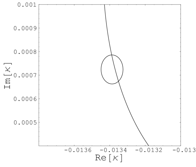
Figure 1: Contour plot on complex $\kappa$-plane. The vertical line and the circle correspond to the solutions of Eqs. (8) and (9), respectively.

These outputs at the GUT scale are used as input parameters in order to solve Eqs. (8) and (9). The contours of solutions of each equations are depicted in Fig. 1, where the signs of the input fermion masses have taken as $-$ for $m_{u}$, $m_{c}$, $m_{d}$, and $m_{s}$, and $+$ for $m_{t}$ and $m_{b}$. We find a solution

$$\kappa=-0.0134+0.000786i\;,$$

$$|c_{d}|=6.38\;,$$ (27)

which leads to the reasonable results for the neutrino sector.

Now we can describe all the fermion mass matrices as functions of $\sigma$ and $c_{R}$ by using the above solution through the mass matrix formulas of Eqs. (5), (10) and (11). Since the PMNS mixing angles are independent of $c_{R}$, we can plot the angles as functions of $\sigma$. The results are depicted in Fig. 2, and we can see that the resultant mixing angles are very sensitive to $\sigma$. For $\sigma=3.198[\mbox{rad}]$, we obtain $\sin^{2}2\theta_{12}=0.722$, $\sin^{2}2\theta_{23}=0.881$ and $\sin^{2}2\theta_{13}=0.164$ at the GUT scale. After running this results back to the electroweak scale according to RGE of Eq. (18), we find

$$\sin^{2}2\theta_{12}=0.723,\;\;\sin^{2}2\theta_{23}=0.895,\;\;\sin^{2}2\theta_{13}=0.164\;.$$ (28)

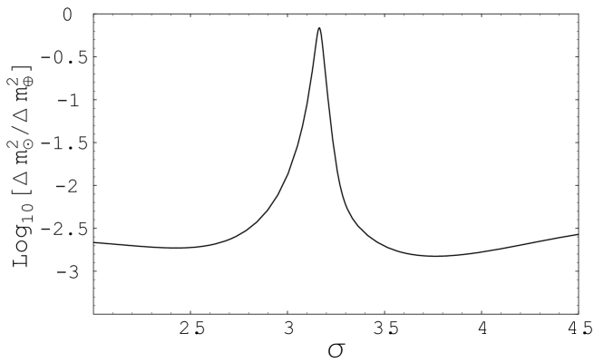
Figure 3: The ratio ($\mbox{Log}_{10}[\Delta m_{\odot}^{2}/\Delta m_{\oplus}^{2}]$) as the function of $\sigma\mbox{[rad]}$.

Note that RGE running effects are almost negligible. The ratio $\Delta m_{\odot}^{2}/\Delta m_{\oplus}^{2}$ is also independent of $c_{R}$, where $\Delta m_{\odot}^{2}$ and $\Delta m_{\oplus}^{2}$ are the oscillation parameters relevant for the solar and the atmospheric neutrino deficits, respectively. In Fig. 3, the ratio at the GUT scale is depicted as a function of $\sigma$. After the RGE running, we find, at the electroweak scale,

$$\frac{\Delta m_{\odot}^{2}}{\Delta m_{\oplus}^{2}}=0.188\;.$$ (29)

RGE running effects are almost negligible also for the ratio. The neutrino mass matrix at the electroweak scale and the PMNS matrix which lead to the above results are as follows:

$$M_{\nu}=c_{R}^{-1}\left(\begin{array}[]{ccc}14.7+48.0i&-46.9-96.5i&-446-370i\\ -46.9-96.5i&-347+90.3i&1030+702i\\ -446-370i&1030+702i&-497-914i\end{array}\right)\;(\mbox{GeV})\;,$$ (33)

and

$$U_{PMNS}=\left(\begin{array}[]{ccc}0.168+0.838i&-0.467+0.0940i&-0.00508+0.207i\\ 0.0519+0.498i&0.651-0.0473i&0.0189-0.569i\\ 0.0745+0.116i&0.450-0.381i&0.431+0.669i\end{array}\right)\;.$$ (37)

They have been calculated in the basis where the charged-lepton mass matrix is diagonal and all the matrix elements are real and positive. The neutrino mass eigenvalues are determined by fixing $c_{R}$ appropriately. For example, taking $c_{R}=3.01\times 10^{13}$ leads to $\Delta m_{\odot}^{2}=3.76\times 10^{-4}\mbox{eV}^{2}$ and $\Delta m_{\oplus}^{2}=2.00\times 10^{-3}\mbox{eV}^{2}$. In this case, three mass eigenvalues of the right-handed neutrinos are found to be (in GeV) $M_{R_{1}}=1.64\times 10^{11}$, $M_{R_{2}}=2.50\times 10^{12}$ and $M_{R_{3}}=8.22\times 10^{12}$, respectively. These results are in agreement with the results of the recent neutrino oscillation analysis [21] with the large angle solution with Mikheev-Smirnov-Wolfenstein effect [22] for the solar neutrino deficit.

Our results are very sensitive to the input values of $m_{s}$ and $\delta$. As mentioned above, the solution of Eqs. (8) and (9) exists only if the input values of $m_{s}$ and $\delta$ are appropriately fixed. In Fig. 1, as $m_{s}$ is taken to be larger for fixed $\delta$, the contour of Eq.(8) moves to the left, while the circle moves to the right. Thus, the solution disappears eventually. On the other hand, as $\delta$ is taken to be larger for fixed $m_{s}$, both of the contours move to the left, but the circle moves faster. Eventually, the solution disappears. This disappearance of the solution occurs by several percent changes of the input parameters. Therefore, with fixed $m_{s}$ ($\delta$), $\delta$ ($m_{s}$) is almost determined in order for the solution to exist.

Next let us see a more important parameter dependence. When $\delta$ and $m_{s}$ are fixed appropriately and the solutions are found, we obtain the similar plot as in Fig. 2 for the mixing angles in the PMNS matrix. However, the hight of the peaks depends on the input $\delta$ values. As in the past works [11] [12], we mostly find that the resultant $\sin^{2}2\theta_{23}$ is too small to be consistent with the experimental data. Only the special values of the inputs and $\sigma$ can give the results being in agreement with all the neutrino oscillation data. The reasonable results we found are as follows:

$\tan\beta$	$m_{s}(M_{Z})$	$\delta$	$\sigma$	$\sin^{2}2\theta_{12}$	$\sin^{2}2\theta_{23}$	$\sin^{2}2\theta_{13}$	$\Delta m_{\odot}^{2}/\Delta m_{\oplus}^{2}$
40	0.0718	$93.6^{\circ}$	3.190	0.738	0.900	0.163	0.205
45	0.0729	$86.4^{\circ}$	3.198	0.723	0.895	0.164	0.188
50	0.0747	$77.4^{\circ}$	3.200	0.683	0.901	0.164	0.200
55	0.0800	$57.6^{\circ}$	3.201	0.638	0.878	0.152	0.198

The mass eigenvalues of the light Majorana neutrinos are determined by $c_{R}$. In other words, $c_{R}$ is a function of the oscillation parameter, and appropriate value of $c_{R}$ is fixed so as to be suitable for the neutrino oscillation data. These relations are listed in the following.

$\tan\beta$	$c_{R}\times m_{\nu_{3}}\mbox{(TeV)}~{}$	$~{}c_{R}\times\sqrt{\frac{\Delta m_{\oplus}^{2}}{10^{-3}\mbox{eV}^{2}}}$
40	2.18	$~{}6.26\times 10^{13}$
45	2.08	$~{}6.02\times 10^{13}$
50	1.81	$~{}5.23\times 10^{13}$
55	1.42	$~{}4.04\times 10^{13}$

Here, $m_{\nu_{3}}$ is the mass eigenvalue of the heaviest light Majorana neutrino. As mentioned above, our resultant neutrino oscillation parameters are sensitive to all the input parameters. In other words, if we use the neutrino oscillation data as the input parameters, the other input, for example, the CP-phase in the CKM matrix can be regarded as the prediction of our model. It is a very interesting observation that the CP-phases listed above are in the region consistent with experiments [20].

5 Other predictions

Now all the mass matrices have been completely determined in our model as discussed in the previous section. There are other interesting physical observables which can be calculated by using the concrete fermion mass matrices in our model.

The averaged neutrino mass relevant for the neutrino-less double beta decay [23] can be read off from $(1,1)$ component of the light Majorana neutrino mass matrix $M_{\nu}$. The CP-violation in the lepton sector is characterized by the Jarlskog parameter [24] defined as

$$J_{CP}=\mbox{Im}\left[U_{e2}U_{\mu 2}^{*}U_{e3}^{*}U_{\mu 3}\right]\;,$$ (38)

where $U_{fi}$ is the PMNS matrix element.

It is well known that the SO(10) GUT model possesses a simple mechanism of baryogenesis through the out-of-equilibrium decay of the right-handed neutrinos, namely, the leptogenesis [25]. The amount of the created baryon asymmetry is characterized by the CP-violating parameter $\epsilon$ estimated as

$$\epsilon\sim\sum_{j=2,3}\frac{\mbox{Im}\left[(M_{D}M_{D}^{\dagger})_{1j}^{2}\right]}{v^{2}\sin^{2}\beta(M_{D}M_{D}^{\dagger})_{11}}\frac{M_{R_{1}}}{M_{R_{j}}}\;.$$ (39)

Here, $M_{D}$ is the neutrino Dirac mass matrix in the basis where the right-handed Majorana mass matrix $M_{R}$ is real and diagonal, and $M_{R_{j}}$ is the mass eigenvalue of the right-handed Majorana neutrino of the i-th generation.

These quantities are evaluated by using the results presented in the previous section, and results are listed in the following.

$\tan\beta$	$\langle m_{\nu}\rangle_{ee}~{}(\mbox{eV})$	$J_{CP}$	$\epsilon$
40	0.00122	$~{}~{}0.00110$	$7.39\times 10^{-5}$
45	0.00118	$-0.00429$	$6.80\times 10^{-5}$
50	0.00119	$-0.00631$	$6.50\times 10^{-5}$
55	0.00117	$-0.00612$	$11.2\times 10^{-5}$

Here, $c_{R}$ was fixed so that $\Delta m_{\oplus}^{2}=2\times 10^{-3}\mbox{eV}^{2}$. Unfortunately, both of the averaged neutrino mass and the Jarlskog parameter may be too small to expect their evidences in future experiments. On the other hand, the CP-violating parameter is too large to be consistent with the observed baryon asymmetry. The problem of this too large baryon asymmetry can be easily avoided by assuming an inflationary universe whose reheating temperature is smaller than the right-handed neutrino masses. However, in this case, the leptogenesis scenario no longer works, and another scenario of baryogenesis such as the Affleck-Dine mechanism [26] may be applicable.

Sizable lepton-flavor violation (LFV) can be expected in SUSY models, and the LFV processes are one of the most important processes as the low-energy SUSY search [27]. In detailed analysis, concrete fermion mass matrices are necessary. It is worth investigating the LFV processes in our model.

6 Summary and comments

We have discussed the minimal SUSY SO(10) model, where only one 10 and one $\overline{\bf 126}$ Higgs multiplets have Yukawa couplings with fermions. This model can determine all the fermion mass matrices with only a few free parameters. It is known that, in the absence of CP violation, this model cannot incorporate the realistic neutrino mass matrix consistent with the neutrino oscillation data. We examined more general case in which CP-violating phases in the fermion mass matrices were introduced. In this case, using the experimental data of six quark masses, three angles and one CP-phase in the CKM matrix and three charged-lepton masses, the light Majorana neutrino mass matrix can be determined as the function of only one free parameter $\sigma$ through the GUT relation and the see-saw mechanism. Here we do not count $c_{R}$, which plays only the role to fix the overall scale of the neutrino masses. In order to connect the mass matrix data between the electroweak and the GUT scales, we have analyzed the one-loop RGEs of the charged fermion Yukawa couplings and the effective dimension-five operator of the light Majorana neutrinos.

We found that there was the parameter region in which the predicted neutrino mass matrix can be consistent with the current neutrino oscillation data. This parameter region is severely constrained, and all the parameters, even the CP-phase in the CKM matrix, are almost fixed for given $\tan\beta$. In other words, we can regard the neutrino oscillation data as the inputs while the CP-phase as the output. Interestingly, our results consistent with the neutrino oscillation data are also consistent with experimental results of CP-violation in the quark sector.

In our RGE analysis, we have used RGEs introduced in Sec. 3 at all the energy scales between the electroweak scale and the GUT scale. This treatment fails at the energy larger than the right-handed Majorana neutrino mass scale, where the right-handed neutrinos are no longer decoupled. Above that scale, we have to take RGE of neutrino Yukawa coupling into account. However, as found in Sec. 4, the Majorana mass scale is about $10^{13}\mbox{GeV}$, and close to the GUT scale in the sense of the RGE (logarithmic) running. Thus, we expect that our results can be still reliable. In fact, we can find that changes of our input values at the GUT scale remain within several percents even if the neutrino Yukawa coupling RGE is taken into account, and that the results presented in Sec. 4 are almost unchanged.

In addition, we have neglected the SUSY threshold corrections in our RGE analysis. It is known that with large $tan\beta$ the down-type quark mass matrix is potentially affected by large SUSY threshold corrections and we can neglect them with a limited region of the soft SUSY breaking parameters [28]. If the SUSY threshold corrections are large, it should be taken into account in our analysis, and will change the input values at the GUT scale and eventually the final result. It is an interesting question whether the result gives a better or worse fit, and it is worth analyzing the RGEs taking SUSY threshold corrections into account.

When the CHOOZ data [29] is concerned, our results seems to be in sever situation [30]. However, more comprehensive analysis [31] gives rather loose constraint. In any case, our results lie in the allowed region at 99% C.L. in the global analysis [21], and we have concluded that they are in agreement with the current neutrino oscillation data. This situation seems to be inevitable in our model, since two angles, $\sin^{2}2\theta_{23}$ and $\sin^{2}2\theta_{13}$, are strongly correlated and have the peaks at almost the same $\sigma$ value as can be seen in Fig. 2. This can be easily avoided, when we extend the minimal model and introduce new Higgs multiplets. An extended model has new free parameters in fermion mass matrices, and can be in much better agreement with the neutrino oscillation data, larger $\sin^{2}2\theta_{23}$ but smaller $\sin^{2}2\theta_{13}$. However, what we have found in this paper is that the minimal SO(10) model, the model with only minimal set of Higgs multiplets, is still viable without any extention.

We have concentrated our discussion only on the Yukawa sector with one ${\bf 10}$ and one $\overline{\bf 126}$ Higgs multiplets. In order to complete our model, it is necessary to construct a concrete Higgs sector which can realize all the assumptions in our model, the correct GUT symmetry breaking, doublet-doublet (triplet) Higgs mass splitting etc. Such a Higgs sector may include new Higgs multiplets which affect the fermion mass matrices. If it is the case, our model becomes less predictive, although the model can be in better agreement with the neutrino oscillation data. This issue is highly non-trivial, and a further work is needed.

Although, in this paper, the SUSY SO(10) model has been considered, non-SUSY SO(10) model with intermediate symmetry breaking scales is also worth investigating. In this case, the strategy is completely analogous to that we discussed in this paper, except that RGEs are replaced by the ones of non-SUSY case.

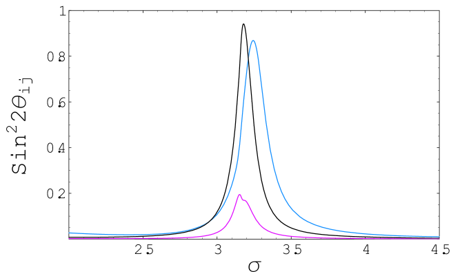
Figure 2: Three mixing angles in the PMNS matrix as functions of $\sigma\mbox{[rad]}$. The graphs with the highest, middle and lowest peaks correspond to $\sin^{2}2\theta_{23}$, $\sin^{2}2\theta_{12}$ and $\sin^{2}2\theta_{13}$, respectively. The plots of $\sin^{2}2\theta_{23}$ and $\sin^{2}2\theta_{13}$ have the sharp peaks at $\sigma\sim 3.2[\mbox{rad}]$, while $\sin^{2}2\theta_{12}$ has the sharp peak at $\sigma\sim 3.3[\mbox{rad}]$.

References

- [1] See, for example, H. P. Nilles, Phys. Rept. 110, 1 (1984), and references therein.
- [2] C. Giunti, C. W. Kim and U. W. Lee, Mod. Phys. Lett. A 6, 1745 (1991); P. Langacker and M. x. Luo, Phys. Rev. D 44, 817 (1991); U. Amaldi, W. de Boer and H. Furstenau, Phys. Lett. B 260, 447 (1991).
- [3] Homestake Collaboration, K. Lande, talk at the 19th International Conference on Neutrino Physics and Astrophysics, Sudbury, Canada, June 16-21, 2000.
- [4] Y. Fukuda et al. [Kamiokande Collaboration], Phys. Rev. Lett. 77, 1683 (1996).
- [5] J. N. Abdurashitov et al. [SAGE Collaboration], Phys. Rev. C 60, 055801 (1999) [arXiv:astro-ph/9907113].
- [6] W. Hampel et al. [GALLEX Collaboration], Phys. Lett. B 447, 127 (1999); M. Altmann et al. [GNO Collaboration], Phys. Lett. B 490, 16 (2000) [arXiv:hep-ex/0006034].
- [7] S. Fukuda et al. [Super-Kamiokande Collaboration], Phys. Rev. Lett. 86, 5656 (2001) [arXiv:hep-ex/0103033]; S. Fukuda et al. [SuperKamiokande Collaboration], Phys. Rev. Lett. 86, 5651 (2001) [arXiv:hep-ex/0103032].
- [8] Q. R. Ahmad et al. [SNO Collaboration], Phys. Rev. Lett. 87, 071301 (2001) [arXiv:nucl-ex/0106015].
- [9] Y. Fukuda et al. [Super-Kamiokande Collaboration], Phys. Rev. Lett. 81, 1562 (1998) [arXiv:hep-ex/9807003]; T. Toshito [SuperKamiokande Collaboration], arXiv:hep-ex/0105023.
- [10] T. Yanagida, in Proceedings of the workshop on the Unified Theory and Baryon Number in the Universe, edited by O.Sawada and A.Sugamoto (KEK, Tsukuba, 1979); M. Gell-Mann, P. Ramond, and R. Slansky, in Supergravity, edited by D.Freedman and P.van Niewenhuizen (north-Holland, Amsterdam 1979); R. N. Mohapatra and G. Senjanovic, Phys. Rev. Lett. 44, 912 (1980).
- [11] K. S. Babu and R. N. Mohapatra, Phys. Rev. Lett. 70, 2845 (1993) [arXiv:hep-ph/9209215].
- [12] D. G. Lee and R. N. Mohapatra, Phys. Rev. D 51, 1353 (1995) [arXiv:hep-ph/9406328].
- [13] K. Matsuda, Y. Koide, T. Fukuyama and H. Nishiura, Phys. Rev. D 65, 033008 (2002) [Erratum-ibid. D 65, 079904 (2002)] [arXiv:hep-ph/0108202].
- [14] P. H. Chankowski and Z. Pluciennik, Phys. Lett. B 316, 312 (1993) [arXiv:hep-ph/9306333]; K. S. Babu, C. N. Leung and J. Pantaleone, Phys. Lett. B 319, 191 (1993) [arXiv:hep-ph/9309223]; S. Antusch, M. Drees, J. Kersten, M. Lindner and M. Ratz, Phys. Lett. B 519, 238 (2001) [arXiv:hep-ph/0108005]; S. Antusch, M. Drees, J. Kersten, M. Lindner and M. Ratz, Phys. Lett. B 525, 130 (2002) [arXiv:hep-ph/0110366].
- [15] J. C. Pati and A. Salam, Phys. Rev. D 10, 275 (1974).
- [16] H. Georgi and C. Jarlskog, Phys. Lett. B 86, 297 (1979).
- [17] K. Matsuda, Y. Koide and T. Fukuyama, Phys. Rev. D 64, 053015 (2001) [arXiv:hep-ph/0010026].
- [18] See, for example, D. J. Castano, E. J. Piard and P. Ramond, Phys. Rev. D 49, 4882 (1994) [arXiv:hep-ph/9308335].
- [19] H. Fusaoka and Y. Koide, Phys. Rev. D 57, 3986 (1998) [arXiv:hep-ph/9712201].
- [20] D. E. Groom et al. [Particle Data Group Collaboration], Eur. Phys. J. C 15, 1 (2000).
- [21] M. C. Gonzalez-Garcia, M. Maltoni, C. Pena-Garay, J. W. F. Valle Phys. Rev. D 63, 033005, (2001) [arXiv:hep-ph/0009350]; G. L. Fogli, E. Lisi, D. Montanino and A. Palazzo, Phys. Rev. D 64, 093007 (2001) [arXiv:hep-ph/0106247]; J. N. Bahcall, M. C. Gonzalez-Garcia and C. Pena-Garay, JHEP 0108, 014 (2001) [arXiv:hep-ph/0106258].
- [22] S. P. Mikheev and A. Y. Smirnov, Sov. J. Nucl. Phys. 42, 913 (1985) [Yad. Fiz. 42, 1441 (1985)]; L. Wolfenstein, Phys. Rev. D 17, 2369 (1978).
- [23] M. Doi, T. Kotani and E. Takasugi, Prog. Theor. Phys. Suppl. 83, 1 (1985).
- [24] C. Jarlskog, Phys. Rev. Lett. 55, 1039 (1985).
- [25] M. Fukugita and T. Yanagida, Phys. Lett. B 174, 45 (1986).
- [26] I. Affleck and M. Dine, Nucl. Phys. B 249, 361 (1985).
- [27] For a recent review, see, for example, J. Hisano, arXiv:hep-ph/0204100, and references therein.
- [28] L. J. Hall, R. Rattazzi and U. Sarid, Phys. Rev. D 50, 7048 (1994) [arXiv:hep-ph/9306309]; M. Carena, M. Olechowski, S. Pokorski and C. E. Wagner, Nucl. Phys. B 426, 269 (1994) [arXiv:hep-ph/9402253]; R. Hempfling, Z. Phys. C 63, 309 (1994) [arXiv:hep-ph/9404226]; T. Blazek, S. Raby and S. Pokorski, Phys. Rev. D 52, 4151 (1995) [arXiv:hep-ph/9504364].
- [29] M. Apollonio et al. [CHOOZ Collaboration], Phys. Lett. B 466, 415 (1999) [arXiv:hep-ex/9907037].
- [30] S. M. Bilenky, D. Nicolo and S. T. Petcov, arXiv:hep-ph/0112216.
- [31] M. C. Gonzalez-Garcia and M. Maltoni, arXiv:hep-ph/0202218; See also the comprehensive report on this by E. Lisi in Neutrino 2002, http://neutrino.t30.physik.tu-muenchen.de/pages/transparencies/ .