Electric Flux Sectors and Confinement

Abstract

We study the fate of static fundamental charges in the thermodynamic limit from Monte-Carlo simulations of $SU(2)$ with suitable boundary conditions.

1 Introduction

In QED, the charge of a particle is of long-range nature. It can exist because the photon is massless. Localized objects are neutral like atoms. Within the language of local field-systems one derives more generally that every gauge-invariant localized state is singlet under the unbroken charges of global gauge invariance. Thus, without (electric) Higgs mechanism, QED and QCD have in common that any localized physical state must be chargeless/colorless.

The extension to all physical states is possible only with a mass gap. Without that, in QED, non-local charged states which are gauge-invariant can arise as limits of local ones which are not. The Hilbert space decomposes into the so-called superselection sectors of the physical states with different charges. With a mass gap in QCD, on the other hand, color-electric charge superselection sectors cannot arise: every gauge-invariant state can be approximated by gauge-invariant localized ones (which are colorless). One concludes that every gauge-invariant state must also be a color singlet.

On the other hand, charged states are always possible with suitable boundary conditions in a finite volume. This allows to study their fate in the thermodynamic limit from Monte-Carlo simulations on finite lattices. In an Abelian theory for example, anti-periodic (spatial) boundary conditions can be used to force the system into a charged sector in the infinite volume limit [1]. The (Higgs vs. Coulomb) phases of the non-compact Abelian Higgs model can be distinguished in this way. And by duality, via the ZZ gauge theory, the magnetic sectors of compact $U(1)$ follow an analogous pattern. The difference in free energy of the anti-periodic vs. the periodic ensemble thereby tends to zero or a finite value for the (magnetic) Higgs or Coulomb phases, respectively.

In pure $SU(N)$ gauge theory, one expects the free energy $F_{q}(T,L)$ of a static fundamental charge in a $1/T\times L^{3}$ box, for $L\!\to\!\infty$, to jump from $\infty$ to a finite value at $T\!=\!T_{c}$ reflecting the deconfinement transition. The Polyakov loop $P$ is commonly used to demonstrate this in lattice studies. If $\langle P\rangle\equiv e^{-F_{q}/T}\!$, the center symmetric (broken) phase gives for $F_{q}$ an infinite (finite) value. However, the periodic boundary conditions (b.c.) within which $\langle P\rangle$ is measured are incompatible with the presence of a single charge also in this case. And, like any Wilson loop, $\langle P\rangle$ is subject to UV-divergent perimeter terms, such that $\langle P\rangle=0$ at all $T$ as the lattice spacing $a\!\rightarrow\!0$.

Following [2], it is possible, however, to measure the gauge-invariant, UV-regular free energy of a static fundamental charge [3, 4], and show that it has the expected behaviour, dual to that of temporal center flux [5]. The preparation of suitable b.c.’s to achieve this is a little indirect.

2 Twist vs. Electric Flux Sectors in $SU(2)$

For the different sectors relevant to the confinement transition in pure $SU(N)$ gauge theory, one needs to distinguish between the finite volume partition functions of two types.

First, ’t Hooft’s twisted boundary conditions fix the total number of $\mbox{\sf Z\mbox{}Z}_{N}$-vortices modulo $N$ that pierce planes of a given orientation. On the 4-dimensional torus $T^{4}$ there are $N^{6}$ different such sectors corresponding to the 6 possible orientations for the planes of the twists. Without fields that faithfully represent the center $\mbox{\sf Z\mbox{}Z}_{N}$ of $SU(N)$, the structure is $G=SU(N)/\mbox{\sf Z\mbox{}Z}_{N}$ with first homotopy $\pi_{1}(G)=\mbox{\sf Z\mbox{}Z}_{N}$. The $N^{6}$ inequivalent choices for imposing (twisted) boundary conditions on the gauge potentials $A$ therefore correspond to the classification of the bundles, by their $\mbox{\sf Z\mbox{}Z}_{N}$-vortex numbers, according to the harmonic 2-forms over $T^{4}$ with $\pi_{1}(G)=\mbox{\sf Z\mbox{}Z}_{N}$ coefficients, the 2nd de Rahm cohomology group $H^{2}(T^{4},\mbox{\sf Z\mbox{}Z}_{N})$.

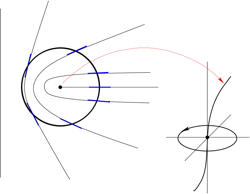
3d-line defect: $\mbox{\sf Z\mbox{}Z}_{2}$-vortex, maps circle to a non-contractible loop in $\mbox{\mbox{\hskip 0.70004pt}\rule{0.27995pt}{4.82224pt}\mbox{}{\sf R}}P(2)$, same happens in $SO(3)\!=\!SU(2)/\mbox{\sf Z\mbox{}Z}_{2}$.

Figure 1: 3d $\mbox{\sf Z\mbox{}Z}_{2}$-vortex as in, e.g., nematic liquid crystals (left). Assume the 4d-vortices can lower their free energy by spreading (right): they can do that in the 3 spatial $\vec{m}$-planes at all $T$ (top), while they are squeezed in the 3 temporal $\vec{k}$-planes at large $T$ (bottom).

At finite temperature $T>0$ the $N^{6}$ possible twists come in two classes: 3 temporal ones classified by a vector $\vec{k}\in\mbox{\sf Z\mbox{}Z}_{N}^{3}$, and 3 magnetic ones by $\vec{m}\in\mbox{\sf Z\mbox{}Z}_{N}^{3}$, see Fig. 1. Magnetic twist is defined in purely spatial planes and fixes the conserved, $\mbox{\sf Z\mbox{}Z}_{N}$-valued and gauge-invariant magnetic flux $\vec{m}$ in the perpendicular directions.

The different choices of twisted b.c.’s lead to sectors of fractional Chern-Simons number ($\nu+\vec{k}\cdot\vec{m}/N$) [6] with states labelled by $|\vec{k},\vec{m},\nu\rangle$, where $\nu\in\mbox{\sf Z\mbox{}Z}$ is the usual instanton winding number. These sectors are connected by homotopically non-trivial gauge transformations $\Omega[\vec{k},\nu]$,

$$\Omega[\vec{k}^{\prime},\nu^{\prime}]\,|\vec{k},\vec{m},\nu\rangle\,=\,|\vec{k}\!+\!\vec{k}^{\prime},\vec{m},\nu\!+\!\nu^{\prime}\rangle\,.$$ (1)

A Fourier transform of the twist sectors $Z_{k}(\vec{k},\vec{m},\nu)$, which generalizes the construction of $\theta$-vacua as Bloch waves from $\nu$-vacua in two ways, by replacing $\nu\to(\nu+\vec{k}\cdot\vec{m}/N)$ for fractional winding numbers and with an additional $\mbox{\sf Z\mbox{}Z}_{N}^{3}$-Fourier transform w.r.t. the temporal twist $\vec{k}$, yields,

$$Z_{e}(\vec{e},\vec{m},\theta)\,=\,e^{-\frac{1}{T}F_{e}(\vec{e},\vec{m},\theta)}\,=\,\frac{1}{N^{3}}\,\sum_{\vec{k},\,\nu}\,e^{-i\omega(\vec{k},\nu)}\,Z_{k}(\vec{k},\vec{m},\nu)\,.$$ (2)

Up to a geometric phase $\omega(\vec{k},\nu)=2\pi\vec{e}\cdot\vec{k}/N+\theta(\nu\!+\!\vec{k}\cdot\vec{m}/N)$, the states in the new sectors are then invariant under the non-trivial $\Omega[\vec{k},\nu]$ also,

$$\Omega[\vec{k},\nu]\,|\vec{e},\vec{m},\theta\rangle\,=\,\exp\{i\omega(\vec{k},\nu)\}\,|\vec{e},\vec{m},\theta\rangle\,.$$ (3)

Their partition functions $Z_{e}$ are classified, in addition to their magnetic flux $\vec{m}$ and vacuum angle $\theta$, by their $\mbox{\sf Z\mbox{}Z}_{N}$-valued gauge-invariant electric flux in the $\vec{e}$-direction [2]. Here, we do not consider finite $\theta$ which we omit henceforth. Recall the following points for details of which we refer to [3]:

(i) The twisted partition functions, relative to the periodic ensemble $Z_{k}(0,0)$, are expectation values of combinations of ’t Hooft loops $\widetilde{W}$ of maximal size in $(\mu,\nu)$-planes dual to the planes of the twists,

$${Z_{k}(\vec{k},\vec{m})}/{Z_{k}(0,0)}=\langle{\widetilde{W}}^{\rm max}_{(\mu,\nu)}\,\rangle\;.$$ (4)

In particular, the temporal $\vec{k}$-twists correspond to expectation values of spatial ’t Hooft loops. The $\mbox{\sf Z\mbox{}Z}_{N}^{3}$-Fourier transform of Eq. (2) exhibits their Kramers-Wannier duality with the electric flux sectors which are expectation values of Polyakov loops in the no-flux ensemble $Z_{e}(0,0)$ (see below).

(ii) Note also that the no-flux ensemble in a finite volume is manifestly different from the periodic ensemble, e.g., for $SU(2)$ one has,

$$Z_{e}(0,0)=\frac{Z_{k}(0,0)}{8}\Big{(}1+3\langle{\widetilde{W}}^{\rm max}_{1,\rm spat}\,\rangle+3\langle{\widetilde{W}}^{\rm max}_{2,\rm spat}\,\rangle+\langle{\widetilde{W}}^{\rm max}_{3,\rm spat}\,\rangle\Big{)}$$ (5)

The combinations of spatial ’t Hooft loops needed to compute this, or any of the electric flux partition functions $Z_{e}(\vec{e},0)$, are sketched in Fig. 2.

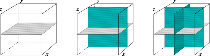
Figure 2: Cubes with one, two, and three $L\!\times\!L$ planes dual to the stacks of plaquettes flipped for temporal twist $\vec{k}=(0,0,1)$, $\vec{k}=(0,1,1)$, and $\vec{k}=(1,1,1)$, from left to right.

(iii) From the gauge-invariant definition of the Polyakov loop $P(\vec{x})$ in presence of temporal twist [7], it is relatively simple but important to verify that the electric-flux partition functions are indeed expectation values of $P$’s in the no-flux ensemble [3], which follow the general pattern,

$$\frac{Z_{e}(\vec{e},0)}{Z_{e}(0,0)}=\big{\langle}P(\vec{x})P^{\dagger}(\vec{x}+L\vec{e})\big{\rangle}_{L,T}\stackrel{{\scriptstyle L\to\infty}}{{\longrightarrow}}\left\{{0\,,\;\;\langle{\widetilde{W}}^{\rm max}_{i,\rm spat}\,\rangle\to 1\,,\;T<T_{c}\atop 1\,,\;\;\langle{\widetilde{W}}^{\rm max}_{i,\rm spat}\,\rangle\to 0\,,\;T>T_{c}}\right.$$ (6)

with $\vec{e}\in\mbox{\sf Z\mbox{}Z}_{N}^{3}$ again. For $\vec{e}\not=0$ this therefore yields the free energy $F_{q}(T,L)=F_{e}(\vec{e},0)$ of one static fundamental charge in the volume $L^{3}$ with b.c.’s such that its electric flux is directed towards its ‘mirror’ (anti)charge in the adjacent volume along the direction of $\vec{e}$. Also note that the operator in the expectation value of (6) has no perimeter, is UV-regular, and one can see in Fig. 3 that there is no Coulomb term for small volumes either.

Of course, Eq.(6) reflects the different realizations of the electric $\mbox{\sf Z\mbox{}Z}_{N}^{3}$ center symmetry in the respective phases. As compared to spin correlations of the form $\langle s_{\vec{x}}\,s_{\vec{x}+L\vec{e}_{i}}\rangle$ in the 3d-Ising model with interfaces, the Polyakov loops in (6) are the corresponding variables in $SU(2)$, whose behavior as a function of temperature is reversed.

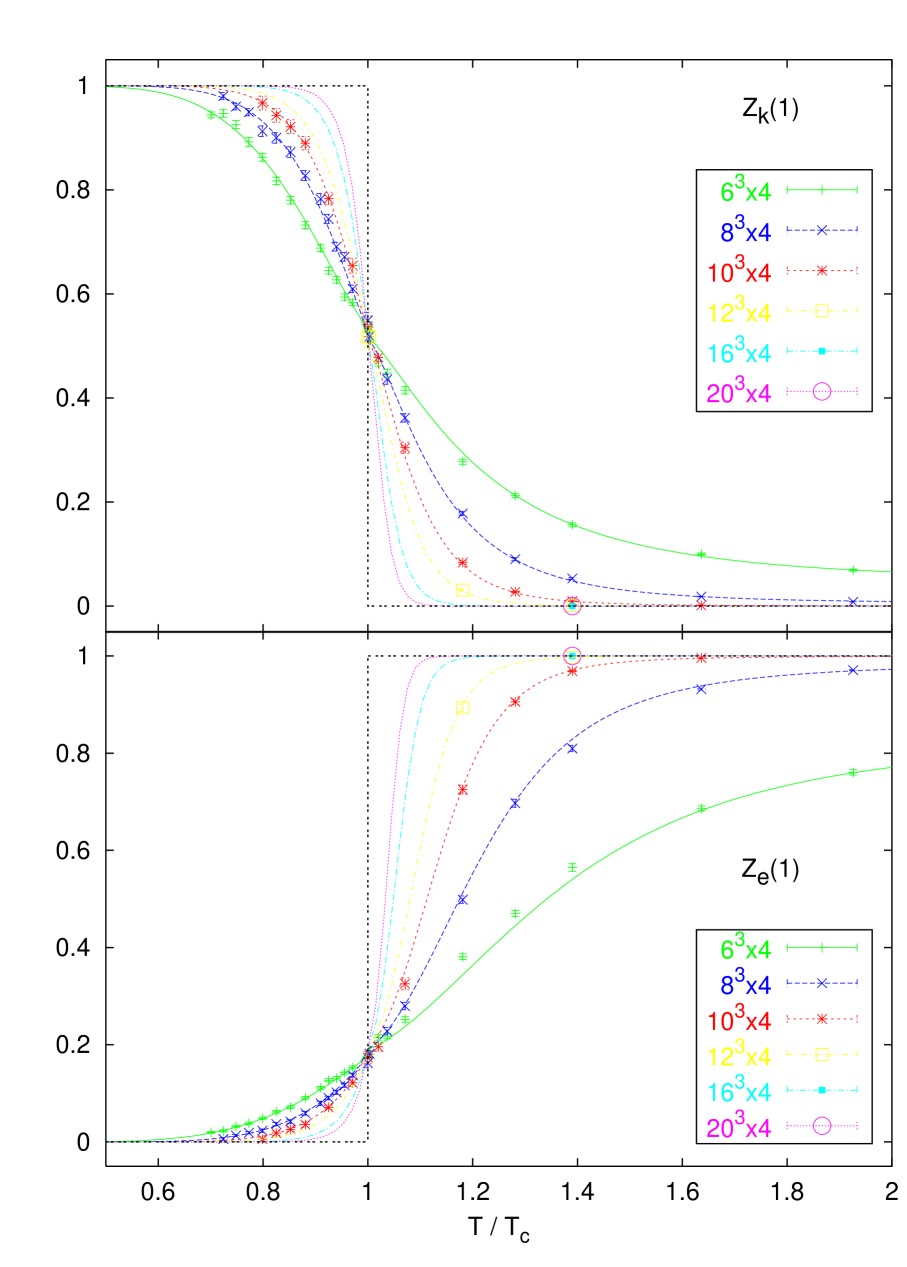
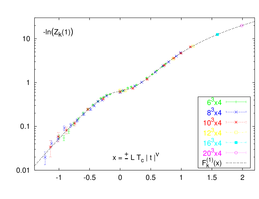
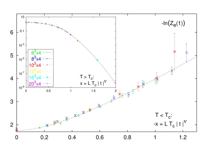
Figure 3: Partition function and free energy of temporal twist (top) and electric flux (bottom), both over temperature (left) and finite size scaling variable $x$ (right).

The dual of the Ising model on the other hand is the 3d $\mbox{\sf Z\mbox{}Z}_{2}$ gauge theory. Interfaces in the first are Wilson loops in the latter. Through duality, the expectation value of a $\mbox{\sf Z\mbox{}Z}_{2}$-Wilson loop along $C$ is expressed as ratio of Ising-model partition functions with and without antiferromagnetic bonds at links dual to a surface $\Omega$, the $\mbox{\sf Z\mbox{}Z}_{2}$-interface, bounded by $C$, e.g., see [8],

$$\big{\langle}W_{\mbox{\sf Z\mbox{}Z}_{2}}(C)\big{\rangle}=\frac{\sum_{\{s\}}\exp\sum_{<ij>}\beta_{ij}\,s_{i}s_{j}}{\sum_{\{s\}}\exp\beta\sum_{<ij>}s_{i}s_{j}}\;,\;\;\beta_{ij}=\Bigg{\{}{-\beta\;,\;\;<\!ij\!>\in\Omega^{*}\atop\phantom{-}\beta\;,\;\;<\!ij\!>\not\in\Omega^{*}}\;.$$ (7)

In $SU(2)$, the objects dual to the Polyakov loop correlations, or the electric fluxes in (6), are spatial ’t Hooft loops. Via universality, these are the $\mbox{\sf Z\mbox{}Z}_{2}$-Wilson loop analogues. And their expectation values are calculated on the lattice in much the same way, by flipping a coclosed set $\Omega^{*}$ of plaquettes dual to some surface $\Omega$ subtended by the loop $C$,

$$\big{\langle}\widetilde{W}_{SU(2)}(C)\big{\rangle}=\frac{\int dU\exp-\sum_{\mathop{\kern 1.0pt\raise-2.0pt\hbox{${\vbox{\hrule height=0.4pt\hbox{\vrule width=0.4pt,height=3.0pt\kern 3.0pt\vrule width=0.4pt} \hrule height=0.4pt}}$}\kern 1.0pt}}\beta(\mathop{\kern 1.0pt\hbox{${\vbox{\hrule height=0.4pt\hbox{\vrule width=0.4pt,height=5.0pt\kern 5.0pt\vrule width=0.4pt} \hrule height=0.4pt}}$}\kern 1.0pt})\mbox{Tr}\,U\!_{\mathop{\kern 1.0pt\raise-2.0pt\hbox{${\vbox{\hrule height=0.4pt\hbox{\vrule width=0.4pt,height=3.0pt\kern 3.0pt\vrule width=0.4pt} \hrule height=0.4pt}}$}\kern 1.0pt}}}{\int dU\exp-\beta\sum_{\mathop{\kern 1.0pt\raise-2.0pt\hbox{${\vbox{\hrule height=0.4pt\hbox{\vrule width=0.4pt,height=3.0pt\kern 3.0pt\vrule width=0.4pt} \hrule height=0.4pt}}$}\kern 1.0pt}}\mbox{Tr}\,U\!_{\mathop{\kern 1.0pt\raise-2.0pt\hbox{${\vbox{\hrule height=0.4pt\hbox{\vrule width=0.4pt,height=3.0pt\kern 3.0pt\vrule width=0.4pt} \hrule height=0.4pt}}$}\kern 1.0pt}}}\;,\;\;\beta(\mathop{\kern 1.0pt\hbox{${\vbox{\hrule height=0.4pt\hbox{\vrule width=0.4pt,height=5.0pt\kern 5.0pt\vrule width=0.4pt} \hrule height=0.4pt}}$}\kern 1.0pt})=\Bigg{\{}{-\beta\;,\;\;\mathop{\kern 1.0pt\hbox{${\vbox{\hrule height=0.4pt\hbox{\vrule width=0.4pt,height=5.0pt\kern 5.0pt\vrule width=0.4pt} \hrule height=0.4pt}}$}\kern 1.0pt}\in\Omega^{*}\atop\phantom{-}\beta\;,\;\;\mathop{\kern 1.0pt\hbox{${\vbox{\hrule height=0.4pt\hbox{\vrule width=0.4pt,height=5.0pt\kern 5.0pt\vrule width=0.4pt} \hrule height=0.4pt}}$}\kern 1.0pt}\not\in\Omega^{*}}\;.$$ (8)

In both cases the surface is arbitrary except for its boundary $C=\partial\Omega$.

A spatial ’t Hooft loop of maximal size $L\times L$, living in, say, the $(x,y)$ plane of the dual lattice, is equivalent to an odd number of flipped plaquettes in every $(z,t)$ plane of the original lattice. This enforces twisted b.c.’s in $(z,t)$. Combining such loops yields the other $\vec{k}$-twist sectors, c.f., Fig. 2.

The temperature dependences of the partition functions for temporal twist $\vec{k}\!=\!(0,0,1)$ and electric flux $\vec{e}\!=\!(0,0,1)$ as calculated in [3] are compared in Fig. 3. Their dual behavior is obvious: for $L\!\to\!\infty$, both approach step functions jumping from 1 to 0 and 0 to 1, respectively, as $T_{c}$ is crossed (from below). Near the phase transition, this behavior is determined by critical exponents and likewise universal amplitude ratios of the 3d-Ising class. For the larger spatial lattice sizes, the fits in the left part of Fig. 3 might look rather daring at first. However, each of the two families of curves shown there really represent one of the unique functions in the right part which fit all the data. This is possible due to finite size scaling.

3 Finite-Size Scaling

Finite size scaling (FSS) laws are based on the observation that the length of the system $L$ and the correlation lengths $\xi$ that diverge in the thermodynamic limit are the only relevant length scales in the neighborhood of the transition. In particular, as the critical point is approached, the finite lattice spacing $a$ becomes less and less important. For the continuous (2nd order) transition of $SU(2)$ in the 3d-Ising class, with $\xi_{\pm}(t)=\xi^{0}_{\pm}|t|^{\nu}$ for reduced temperature $t\mathrel{\hbox to0.0pt{\lower 2.0pt\hbox{\small\hskip 1.0pt$<$}\hss}\hskip 1.0pt\raise 3.0pt\hbox{\small$>$}}0$, we use $t=T/T_{c}-1$ and $\nu=0.63$. And as for the ratios of 3d-Ising model partition functions $Z_{a}/Z_{p}$ with anti-periodic vs. periodic b.c.’s [9], we assume the $L$, $T$ dependence of the various temporal twist sectors, denoting $Z_{k}(i)=\langle{\widetilde{W}}^{\rm max}_{i,\rm spat}\,\rangle$ for $i=1,..3$ orthogonal $\vec{k}$-twists, to be governed by simple FSS laws,

$$\hskip 28.45274ptZ_{k}(i)\,=\,f^{(i)}(x)\;,\;\;\mbox{with}\;\;x=\pm LT_{c}|t|^{\nu}\propto L/\xi_{\pm}(t)\;,\;\mbox{for}\;t\mathrel{\hbox to0.0pt{\lower 2.0pt\hbox{\small\hskip 1.0pt$<$}\hss}\hskip 1.0pt\raise 3.0pt\hbox{\small$>$}}0\;.$$ (9)

We then observe that our results over $x$ for all different lattice sizes nicely collapse on a single curve, c.f., Fig. 3. In the high temperature phase above $T_{c}$, the large-$x$ behavior, $-\ln f^{\scriptscriptstyle(i)}(x)=\tilde{\sigma}_{0}^{\scriptscriptstyle(i)}\,x^{2}+\dots$, reflects the dual area law for ($i=1,..3$) large spatial ’t Hooft loops. Their dual string tension,

$$\tilde{\sigma}(t)=\tilde{\sigma}_{0}^{\scriptscriptstyle(1)}T_{c}^{2}\;t^{2\nu}\,=\,R/\xi_{+}^{2}(t)\;,$$ (10)

is the Ising analogue of the interface tension $\sigma_{I}(t)=R/\xi_{-}^{2}(t)\sim|t|^{2\nu}$ below $T_{c}$, where $R\simeq 0.104$ is a universal ratio [10, 11]. In addition, the universality hypothesis relates the ratio of the correlation lengths for the Polyakov loops in $SU(2)$ to the correlation lengths of the spins in the 3d-Ising model, as measured in [11],

$$\xi_{-}^{SU(2)}/\xi_{+}^{SU(2)}\,\stackrel{{\scriptstyle!}}{{=}}\,\xi_{+}^{\mbox{\tiny Ising}}/\xi_{-}^{\mbox{\tiny Ising}}\,\simeq\,1.96\;.$$ (11)

Together with the large-$x$ asymptotics of $i=1,..3$ electric fluxes, $-\!\ln Z_{e}(i)=\sigma_{0}^{\scriptscriptstyle(i)}|x|+\dots$, below $T_{c}$, this relates the string tension amplitude $\sigma_{0}\equiv\sigma_{0}^{\scriptscriptstyle(1)}$ below $T_{c}$ to its dual counterpart $\tilde{\sigma}_{0}\equiv\tilde{\sigma}_{0}^{\scriptscriptstyle(1)}$ above $T_{c}$,

$$\sigma(T)=\sigma_{0}\,T_{c}\,|t|^{\nu}\,T\;,\;\;\mbox{with}\;\;\sigma_{0}=\sqrt{\tilde{\sigma}_{0}/R_{+}}\;,\;\;R_{+}=R\,{\xi_{-}^{2}}/{\xi_{+}^{2}}\,\simeq 0.4\;.$$ (12)

Within the accuracy of our results, the $SU(2)$ data is fully consistent with these ratios. The quite impressive range of universal behavior can be appreciated in comparing the $SU(2)$ temporal twist with the interface free energy $-\ln Z_{a}/Z_{p}$ in the 3d-Ising model [13], see Fig. 4. Once a non-universal constant of proportionality relating both FSS variables is fixed, the scaling functions appear to be identical for the whole range of the $SU(2)$ data (with high and low temperature phases interchanged). The same agreement is observed for all $f^{(i)}(x)$, i.e., also between 2 and 3 orthogonal twists in $SU(2)$ and Ising model with anti-periodic b.c.’s in 2 and 3 directions.

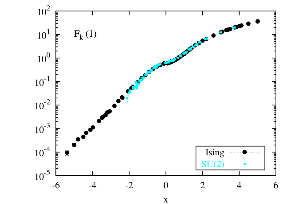
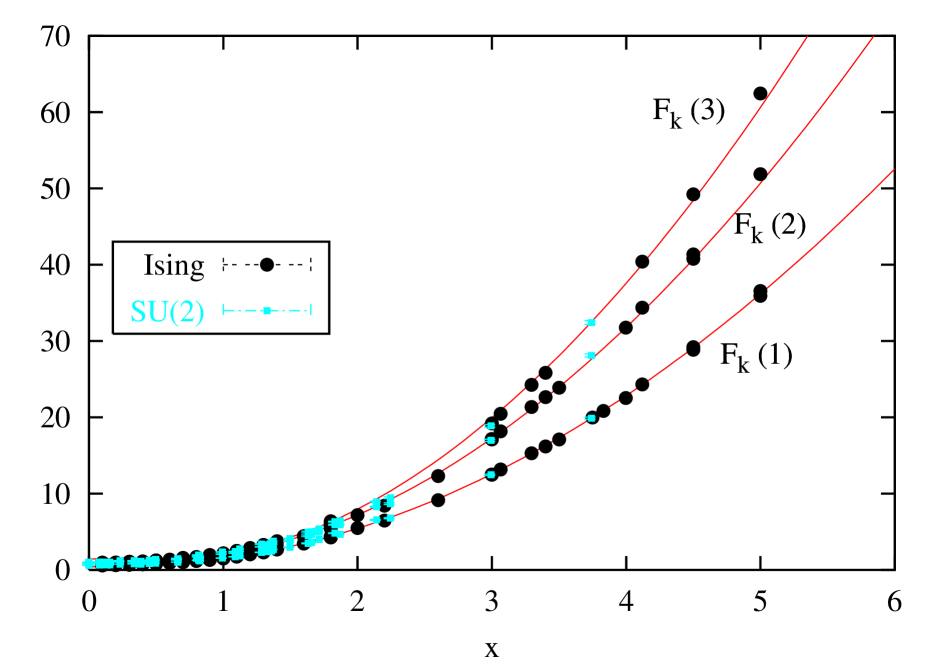
Figure 4: Free energy $F_{k}(1)=-\ln Z_{k}(1)$ of one temporal twist in $SU(2)$, same data as in Fig. 3, compared to that of an interface in the Ising model $F_{k}(1)=-\ln(Z_{a}/Z_{p})$ with $x_{\mbox{\tiny Ising}}=-1.88(2)x_{SU(2)}$ (left); 1-3 orthogonal $\vec{k}$-twists in $SU(2)$ ($T\!>\!T_{c}$) vs. Ising with 1-3 anti-periodic directions ($T\!<\!T_{c}$), with square-root ratios in the fits (right), from [13].

4 String Formation

In the low temperature phase, the formation of electric flux strings is expected. The signature for this are square-root ratios $1:\sqrt{2}:\sqrt{3}$ of the string tension amplitudes $\sigma_{0}^{\scriptscriptstyle(i)}$ for $i=1,2$ and 3 orthogonal fluxes. At $T=0$ the singificance for such a behavior, as compared to the ratios $1:{2}:{3}$ expected for isotropic fluxes, was assessed in the pioneering study of Ref. [12].

Above $T_{c}$ on the other hand, the same square-root ratios for the dual string tension amplitudes,

$$\tilde{\sigma}_{0}^{(1)}:\tilde{\sigma}_{0}^{(2)}:\tilde{\sigma}_{0}^{(3)}\;\sim\;1:\sqrt{2}:\sqrt{3}\;,$$ (13)

signal the formation of interfaces with minimal area. These ratios are well confirmed for spatial ’t Hooft loops in orthogonal planes within the accuracy of our $SU(2)$ data [3], and with considerably higher accuracy also for the 3d-Ising model (for $T<T_{c}$) with anti-periodic b.c.’s in 1,2 and 3 directions [13], which are also compared in Fig. 4.

5 Conclusions

To summarize, we have studied the finite volume partition functions in the sectors of pure $SU(2)$ of two types: Using ’t Hooft’s twisted boundary conditions we first measured the free energies of ensembles with odd numbers of $\mbox{\sf Z\mbox{}Z}_{2}$ center-vortices through temporal planes. From combinations of these we then obtained the sectors of gauge-invariant electric flux, and demonstrated explicitly that, below $T_{c}$, their free energy diverges linearly with the length $L$ of the system. Because spatial twists share their qualitative low-$T$ behavior with the temporal ones considered so far, the free energy of the magnetic fluxes must vanish just as that of temporal twist. This is the magnetic Higgs phase with electric confinement of pure $SU(2)$.

At criticality all free energies rapidly approach their finite $L\to\infty$ limits. Above $T_{c}$, the electric-flux free energies vanish in the thermodynamic limit. The transition is well described by simple finite size scaling laws of the 3d-Ising class. The ratios of the (dual) string tension amplitudes for 1,2 and 3 orthogonal (spatial ’t Hooft loops) electric fluxes (above) below $T_{c}$ indicate the formation of diagonal (interfaces) flux strings.

Both of us would like to express our warm thanks to Š. Olejník and J. Greensite for their great job organizing this stimulating workshop.

References

- [1] Polley, L. and Wiese, U.-J. (1991), Nuclear Physics, B356, pp. 629–654
- [2] ’t Hooft, G. (1979), Nuclear Physics, B153, pp. 141–160; see also, ’t Hooft, G. (1998), in P. van Baal (ed.), Confinement, Duality, and Nonperturbative Aspects of QCD, Plenum Press, New York, pp. 379–386
- [3] de Forcrand, Ph. and von Smekal, L. (2001), preprint, [hep-lat/0107018]
- [4] de Forcrand, Ph. and von Smekal, L. (2002), Nuclear Physics, (PS) 106, pp. 619–621
- [5] Kovács, T. G. and Tomboulis, E. T. (2000), Physical Review Letters, 85, pp. 704–707
- [6] van Baal, P. (1982), Communications in Mathematical Physics, 85, pp. 529–547
- [7] van Baal, P. (1984), PhD Thesis, Rijksuniversiteit te Utrecht
- [8] Savit, R. (1980), Review of Modern Physics, 52, pp. 453–487
- [9] Hasenbusch, M. (1993), Physica A, 197, pp. 423–435
- [10] Klessinger, S. and Münster, G. (1992), Nuclear Physics, B386, pp. 701–714.
- [11] Hasenbusch, M. and Pinn, K. (1997), Physica A, 245, pp. 366–378
- [12] Hasenfratz, A., Hasenfratz, P. and Niedermayer, F. (1990), Nuclear Physics, B329, pp. 739–752
- [13] Pepe, M. and de Forcrand, Ph. (2002), Nuclear Physics, (PS) 106, pp. 914–916