Positivity bounds on generalized parton distributions in impact parameter representation

Abstract

New positivity bounds are derived for generalized (off-forward) parton distributions using the impact parameter representation. These inequalities are stable under the evolution to higher normalization points. The full set of inequalities is infinite. Several particular cases are considered explicitly.

I General form of the positivity bounds on GPDs

Generalized parton distributions (GPDs) MRGDH-94 ; Radyushkin-96 ; Ji-97 ; CFS-97 ; Radyushkin-97 ; Radyushkin-review ; GPV ; BMK-2001 also known as off-forward, skewed, nondiagonal etc. appear in the QCD description of various hard processes e.g. deeply virtual Compton scattering and hard exclusive meson production. Our knowledge about GPDs is poor and any additional theoretical information is of value. From this point of view the positivity bounds are rather important.

GPDs are defined in terms of matrix elements

$$G_{P_{1}i_{1},P_{2}i_{2}}^{\alpha_{1}\alpha_{2}}(x_{1},x_{2})=\langle P_{2},i_{2}|\phi_{\alpha_{2}}^{\dagger}\left(x_{2}\right)\phi_{\alpha_{1}}\left(x_{1}\right)|P_{1},i_{1}\rangle$$

$$-\langle P_{2},i_{2}|P_{1},i_{1}\rangle\langle 0|\phi_{\alpha_{2}}^{\dagger}\left(x_{2}\right)\phi_{\alpha_{1}}\left(x_{1}\right)|0\rangle\,.$$ (1)

Here $|P_{k},i_{k}\rangle$ is a hadron state (with momentum $P_{k}$ and spin/isospin indices $i_{k}$) and the field $\phi_{\alpha_{k}}\left(x_{k}\right)$ describes the annihilation of a parton with momentum fraction $x_{k}$ and with spin/isospin labeled by $\alpha_{k}$. Indices $\alpha_{k}$ also contain information about the type of the parton (quark or gluon). The vacuum subtraction term in the RHS of Eq. (1) can be ignored in practical applications of GPDs with $P_{1}\neq P_{2}$ but this term is important in the derivation of the positivity constraints on GPDs. Parton momentum fractions $x_{i}\equiv k_{i}^{+}/P^{+}$ are normalized with respect to some external fixed scale $P^{+}$ and not to the hadron momenta $P_{1}$ or $P_{2}$. Although notation (1) for GPDs differs from the standard one, we find the form (1) rather convenient for the derivation of positivity bounds and for the analysis of the interplay between the evolution and the positivity properties.

The positivity of the norm in the Hilbert space of states

$$\left\|\sum\limits_{i\alpha}\int\frac{dP^{+}d^{2}P^{\perp}dx}{2P^{+}(2\pi)^{3}}\theta(x)f_{i\alpha}(x,P)\phi_{\alpha}\left(x\right)|P,i\rangle\right\|^{2}\geq 0$$ (2)

leads to the inequality

$$\sum\limits_{i_{1}\alpha_{1}i_{2}\alpha_{2}}\int\frac{dP_{1}^{+}d^{2}P_{1}^{\perp}dx_{1}}{2P_{1}^{+}(2\pi)^{3}}\int\frac{dP_{2}^{+}d^{2}P_{2}^{\perp}dx_{2}}{2P_{2}^{+}(2\pi)^{3}}\theta(x_{1})\theta(x_{2})$$

$$\times\,f_{i_{2}\alpha_{2}}^{\ast}(x_{2},P_{2})f_{i_{1}\alpha_{1}}(x_{1},P_{1})G_{P_{1}i_{1},P_{2}i_{2}}^{\alpha_{1}\alpha_{2}}(x_{1},x_{2})\geq 0\,.$$ (3)

The integration over $x_{1,2}$ is restricted to the positive region

$$x_{1}>0\,,\quad x_{2}>0$$ (4)

where the vacuum term vanishes in the RHS of Eq. (1) so that its subtraction does not violate the positivity. In the case of the antiquark GPDs one should consider the region $x_{1},x_{2}<0$.

Strictly speaking the above expressions have to be written more carefully: in the case of the gauge theories the $P$ exponent should be inserted between parton fields and certain conventions have to be chosen concerning the normalization of the momentum fractions $x_{1},x_{2}$.

Various positivity inequalities for GPDs corresponding to specific choices of the function $f_{i\alpha}(x,P)$ have been already discussed in literature Martin-98 ; Radyushkin-99 ; PST-99 ; Ji-98 ; DFJK-00 ; Burkardt-01 ; Pobylitsa-01 ; Pobylitsa-02 ; Diehl-02 ; Burkardt-02-a ; Burkardt-02-b . The aim of this paper is to analyze inequality (3) with arbitrary functions $f_{i\alpha}(x,P)$.

II Positivity bounds and evolution

It is well known that in the case of forward parton distributions the probabilistic interpretation of the one-loop DGLAP evolution GL-BLP ; AP-77 ; Dokshitzer-77 leads to the stability of the positivity properties under the one-loop evolution to higher normalization points. The generalization of this property for some particular positivity bounds on GPDs was considered in Ref. PST-99 . Let us show modifying the argument of Ref. PST-99 that if at some normalization point inequality (3) holds for all functions $f_{i\alpha}(x,P)$ then after the one-loop evolution

$$\mu\frac{\partial}{\partial\mu}G_{P_{1}i_{1},P_{2}i_{2}}^{\alpha_{1}\alpha_{2}}(x_{1},x_{2};\mu)=g^{2}(\mu)\int dy_{1}dy_{2}$$

$$\times\sum\limits_{\beta_{1}\beta_{2}}K_{\beta_{1}\beta_{2}}^{\alpha_{1}\alpha_{2}}(x_{1},x_{2},y_{1},y_{2})G_{P_{1}i_{1},P_{2}i_{2}}^{\beta_{1}\beta_{2}}(y_{1},y_{2};\mu)$$ (5)

to a higher normalization point inequality (3) is still valid for all $f_{i\alpha}(x,P)$.

Positivity bound (3) involves GPDs $G_{P_{1}i_{1},P_{2}i_{2}}^{\alpha_{1}\alpha_{2}}(x_{1},x_{2};\mu)$ with positive $x_{1},x_{2}>0$ (4). If $x_{1},x_{2}>0$ then the one-loop evolution kernels $K_{\beta_{1}\beta_{2}}^{\alpha_{1}\alpha_{2}}(x_{1},x_{2},y_{1},y_{2})$ differ from zero only in the region

$$y_{k}\geq x_{k}\geq 0\,.$$ (6)

This constraint has a simple physical meaning: a parton with momentum fraction $y_{k}$ can emit a parton with momentum fraction $x_{k}$ only under the condition (6).

The one-loop evolution kernels $K_{\beta_{1}\beta_{2}}^{\alpha_{1}\alpha_{2}}(x_{1},x_{2},y_{1},y_{2})$ for GPDs can be interpreted as perturbative parton-in-parton GPDs. For parton-in-parton GPDs one can repeat the derivation of the inequality (3) arriving at the following inequality holding for any function $h_{\alpha\beta}(x,y)$

$$\sum\limits_{i_{k}\alpha_{k}\beta_{k}}\int\limits_{0}^{\infty}dx_{1}\int\limits_{x_{1}}^{\infty}dy_{1}\int\limits_{0}^{\infty}dx_{2}\int\limits_{x_{2}}^{\infty}dy_{2}h_{\alpha_{2}\beta_{2}}^{\ast}(x_{2},y_{2})$$

$$\times h_{\alpha_{1}\beta_{1}}(x_{1},y_{1})K_{\beta_{1}\beta_{2}}^{\alpha_{1}\alpha_{2}}(x_{1},x_{2},y_{1},y_{2})\geq 0\,.$$ (7)

The diagrammatic interpretation of this inequality is described in Appendix A.

Actually inequality (7) holds only for functions $h_{\alpha\beta}(x,y)$ vanishing at $x=y$ because of the virtual terms proportional to $\delta(x_{1}-y_{1})\delta(x_{2}-y_{2})$ which give a negative contribution to the kernel $K_{\beta_{1}\beta_{2}}^{\alpha_{1}\alpha_{2}}(x_{1},x_{2},y_{1},y_{2})$. If one ignores these terms then the stability of the positivity bound (3) with respect to the evolution (5) upwards in $\mu$ is a consequence of the property (7) of the one-loop evolution kernel. The last step is to notice that after the inclusion of the virtual terms proportional to $\delta(x_{1}-y_{1})\delta(x_{2}-y_{2})$ in the evolution equation, the positivity is still preserved under the evolution upwards. One can use the same argument as in the case of the forward distributions: if at some “critical point” $\mu$ inequality (3) is saturated and becomes an equality for some function $f_{i\alpha}(x,P)$ then at this point the virtual terms proportional to $\delta(x_{1}-y_{1})\delta(x_{2}-y_{2})$ do not contribute to the evolution of the LHS of inequality (3) so that at higher $\mu$ the positivity is again restored by the positive part of the evolution kernel. The details can be found in Appendix B.

III Positivity bounds in the impact parameter representation

The positivity bound (3) contains a multidimensional integral in the LHS and this form is not quite convenient for practical applications. Turning to the impact parameter representation Burkardt-01 ; Diehl-02 ; Burkardt-02-a ; Burkardt-02-b one can simplify this inequality. Let us show how this can be done for quark GPDs. The generalization for gluons is straightforward.

Let us introduce a light-cone vector $n$ and define the light-cone coordinates so that $(nX)=X^{+}$ for any 4-vector $X$. Below for simplicity we shall restrict our analysis to the case of “unpolarized” GPDs defined in terms of the matrix elements of the operator $\bar{\psi}(n\gamma)\psi$

$$\int\frac{d\lambda}{2\pi}\,\exp\left[\frac{1}{2}i\lambda(k^{+}_{1}+k^{+}_{2})\right]$$

$$\times\langle P_{2},\sigma_{2}|\bar{\psi}\left(-\frac{\lambda n}{2}\right)(n\gamma)\psi\left(\frac{\lambda n}{2}\right)|P_{1},\sigma_{1}\rangle$$

$$=F_{\sigma_{2}\sigma_{1}}\left[\frac{k^{+}_{1}+k^{+}_{2}}{P_{1}^{+}+P_{2}^{+}},\frac{P_{1}^{+}-P_{2}^{+}}{P_{1}^{+}+P_{2}^{+}},\frac{2(P_{1}^{+}P_{2}^{\perp}-P_{2}^{+}P_{1}^{\perp})}{P_{1}^{+}+P_{2}^{+}}\right]\,.$$ (8)

The structure of the momentum dependence in the RHS is fixed by the Lorentz invariance. In order to see the relation between the arguments of function $F_{\sigma_{2}\sigma_{1}}$ and the standard notation of X. Ji Ji-98

$$\Delta=P_{2}-P_{1}\,,\quad t=\Delta^{2},\quad\xi=\frac{(nP_{1})-(nP_{2})}{(nP_{2})+(nP_{1})}$$ (9)

one can use the frame where $P_{2}^{\perp}=-P_{1}^{\perp}\equiv\Delta^{\perp}/2$. In this frame the RHS of Eq. (8) is simply $F_{\sigma_{2}\sigma_{1}}(x,\xi,\Delta^{\perp})$.The longitudinal momentum flow corresponding to variables $x,\xi$ is shown in Fig. 1.

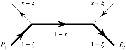
Figure 1: Longitudinal momentum flow corresponding to variables $x,\xi$ [in units of $(P_{1}^{+}+P_{2}^{+})/2$ ].

Let us insert Eq. (8) into the positivity condition (3) and turn to the impact parameter representation

$$\tilde{F}_{\sigma_{2}\sigma_{1}}(x,\xi,b^{\perp})=\int\frac{d^{2}\Delta^{\perp}}{(2\pi)^{2}}\exp\left[i(\Delta^{\perp}b^{\perp})\right]$$

$$\times F_{\sigma_{2}\sigma_{1}}(x,\xi,\Delta^{\perp})\,.$$ (10)

Using a factorized ansatz for the function $f_{i_{1}\alpha_{1}}(x_{1},P_{1})$ one can reduce inequality (3) to the following relatively simple form (technical details can be found in Appendix C)

$$\sum\limits_{\sigma_{1}\sigma_{2}}\,\int\limits_{-1}^{1}d\xi\int\limits_{|\xi|}^{1}dx\frac{1}{(1-x)^{5}}p_{\sigma_{2}}^{\ast}\left(\frac{1-x}{1-\xi}\right)p_{\sigma_{1}}\left(\frac{1-x}{1+\xi}\right)$$

$$\times\tilde{F}_{\sigma_{2}\sigma_{1}}\left(x,\xi,\frac{1-x}{1-\xi^{2}}b^{\perp}\right)\geq 0\,.$$ (11)

This inequality should be valid for any functions $p_{\sigma}$ (originating from the factorized ansatz for $f_{i_{1}\alpha_{1}}(x_{1},P_{1})$) and for any value of parameter $b^{\perp}$ if one wants the original inequality (3) to hold for arbitrary $f_{i_{1}\alpha_{1}}(x_{1},P_{1})$.

For hadrons with spin 0 (e.g. pions) we define the GPD as follows

$$q(x,\xi,t)=\int\frac{d\lambda}{2\pi}\exp\left(i\lambda x\right)$$

$$\times\langle P_{2}|\bar{\psi}\left(-\frac{\lambda n}{2}\right)(n\gamma)\psi\left(\frac{\lambda n}{2}\right)|P_{1}\rangle$$ (12)

and for hadrons with spin 1/2 we use the standard notation of X. Ji Ji-98

$$\int\frac{d\lambda}{2\pi}\exp(i\lambda x)\langle U(P_{2})|\bar{\psi}\left(-\frac{\lambda n}{2}\right)(n\gamma)\psi\left(\frac{\lambda n}{2}\right)|U(P_{1})\rangle$$

$$=H(x,\xi,t)\bar{U}(P_{2})(n\gamma)U(P_{1})$$

$$+\frac{1}{2M}E(x,\xi,t)\bar{U}(P_{2})i\sigma^{\mu\nu}n_{\mu}\Delta_{\nu}U(P_{1})$$ (13)

Here we assume the normalization condition $n(P_{1}+P_{2})=2$. Note that we could not impose this condition earlier since $P_{1}$ and $P_{2}$ were integration variables in Eq. (3). We also follow the standard convention that the transverse coordinates are orthogonal to both $n$ and $P_{1}+P_{2}$. The Lorentz invariant squared momentum transfer $t\equiv\Delta^{2}<0$ can be expressed in terms of the transverse part $|\Delta^{\perp}|^{2}$

$$t=-(1-\xi^{2})^{-1}\left(|\Delta^{\perp}|^{2}+4\xi^{2}M^{2}\right)\,.$$ (14)

In the case of spin-0 hadrons the function $F_{\sigma_{2}\sigma_{1}}$ appearing in inequality (11) can be expressed in terms of GPD $q$ (12) as follows

$$F(x,\xi,\Delta^{\perp})=q\left(x,\xi,-\frac{|\Delta^{\perp}|^{2}+4\xi^{2}M^{2}}{1-\xi^{2}}\right)\,.$$ (15)

For spin-1/2 hadrons we have

$$F_{\sigma_{2}\sigma_{1}}(x,\xi,\Delta^{\perp})=\sqrt{1-\xi^{2}}$$

$$\times\left(\begin{array}[]{cc}2H-\frac{2\xi^{2}}{1-\xi^{2}}E&\frac{-\Delta^{1}+i\Delta^{2}}{M(1-\xi^{2})}E\\ \frac{\Delta^{1}+i\Delta^{2}}{M(1-\xi^{2})}E&2H-\frac{2\xi^{2}}{1-\xi^{2}}E\end{array}\right)_{\sigma_{2}\sigma_{1}}$$ (16)

where the arguments $x,\xi$ and $t$ (14) are assumed for $H$ and $E$ in the RHS.

Inequality (11) is our main result. Combining the expressions for $F_{\sigma_{2}\sigma_{1}}$ in terms of GPDs (15), (16) with the impact parameter representation (10) and inserting the result into inequality (11) one can obtain the explicit form of the inequalities for GPDs $q,H,E$.

IV Positivity bounds on nucleon GPDs

From the practical point of view the most interesting case corresponds to the positivity bounds on nucleon GPDs. Let us rewrite our general inequality (11) for spin-1/2 hadrons in terms of the standard notations for nucleon GPDs $H,E$ (13).

Inserting Eqs. (10) and (16) into the general inequality (11) we find

$$\sum\limits_{\sigma_{1}\sigma_{2}}\,\int\limits_{-1}^{1}d\xi\int\limits_{|\xi|}^{1}dx\frac{\sqrt{1-\xi^{2}}}{(1-x)^{5}}p_{\sigma_{2}}^{\ast}\left(\frac{1-x}{1-\xi}\right)p_{\sigma_{1}}\left(\frac{1-x}{1+\xi}\right)$$

$$\times\int\frac{d^{2}\Delta^{\perp}}{(2\pi)^{2}}\exp\left[i\frac{1-x}{1-\xi^{2}}(\Delta^{\perp}b^{\perp})\right]$$

$$\times\left(\begin{array}[]{cc}2H-\frac{2\xi^{2}}{1-\xi^{2}}E&\frac{-\Delta^{1}+i\Delta^{2}}{M(1-\xi^{2})}E\\ \frac{\Delta^{1}+i\Delta^{2}}{M(1-\xi^{2})}E&2H-\frac{2\xi^{2}}{1-\xi^{2}}E\end{array}\right)_{\sigma_{2}\sigma_{1}}\geq 0\,.$$ (17)

The integration over $\Delta^{\perp}$ can be expressed in terms of the integration over variable $t$ (14). Since functions $p_{\sigma}(z)$ are arbitrary we can rescale them: $p_{\sigma}(z)\rightarrow z^{3/2}p_{\sigma}(z)$. Then inequality (17) takes the form

$$\int\limits_{-1}^{1}d\xi\int\limits_{|\xi|}^{1}\frac{dx}{(1-x)^{2}}\int\limits_{-\infty}^{t_{0}}dt\,J_{0}\left(\frac{1-x}{\sqrt{1-\xi^{2}}}|b^{\perp}|\sqrt{t_{0}-t}\right)$$

$$\times\left\{\left(p_{+,-}^{\ast}p_{+,+}+p_{-,-}^{\ast}p_{-,+}\right)\left(H-\frac{\xi^{2}}{1-\xi^{2}}E\right)\right.$$

$$\left.+\frac{p_{+,-}^{\ast}p_{-,+}+p_{-,-}^{\ast}p_{+,+}}{|b^{\perp}|M(1-x)}\frac{\partial}{\partial t}\left[(t_{0}-t)E\right]\right\}\geq 0\,.$$ (18)

Here $J_{0}$ is the Bessel function, parameter

$$t_{0}=-\frac{4\xi^{2}M^{2}}{1-\xi^{2}}$$ (19)

corresponds to the maximal kinematically allowed value of $t$ (14), functions $H,E$ are taken at their standard arguments $x,\xi,t,$ and $p_{\sigma,\pm}$ are the values of arbitrary functions $p_{\sigma}(z)$ at points $z=(1-x)/(1\pm\xi)$

$$p_{\sigma,\pm}=p_{\sigma}\left(\frac{1-x}{1\pm\xi}\right)\,.$$ (20)

V Special cases

The general positivity bound (11) imposes rather serious constraints on GPDs since it should hold for any functions $p_{\sigma}$ and for any values of the impact parameter $b^{\perp}$. Let us show how choosing various functions $p_{\sigma}$ one can reproduce most of the old positivity bounds and obtain new interesting results. For simplicity we consider the case of spinless hadrons (the generalization for spin-1/2 hadrons is straightforward).

1. Integrating inequality (11) over $b^{\perp}$ with the weight $|b^{\perp}|^{2n}$ and replacing $p(z)\to z^{n+2}p(z)$ we obtain the following inequality for GPD $q$ (15)

$$\int\limits_{-1}^{1}d\xi\int\limits_{|\xi|}^{1}dx\frac{1}{(1-x)^{3}}p^{\ast}\left(\frac{1-x}{1-\xi}\right)p\left(\frac{1-x}{1+\xi}\right)$$

$$\times\left.\frac{\partial^{n}}{\partial t^{n}}q\left(x,\xi,t\right)\right|_{t=-4\xi^{2}M^{2}/(1-\xi^{2})}\geq 0$$ (21)

which should hold for any integer $n=0,1,2,\ldots$ and for any function $p$.

2. Taking $p(z)=\delta(z-c)$ in (11) one arrives at

$$\int\frac{d^{2}\Delta^{\perp}}{(2\pi)^{2}}\exp\left[i(\Delta^{\perp}b^{\perp})\right]\left.q\left(x,0,t\right)\right|_{t=-|\Delta^{\perp}|^{2}}\geq 0\,.$$ (22)

This coincides with the inequality derived earlier in Ref. Burkardt-01 .

3. Using function

$$p\left(z\right)=c_{1}\delta\left(z-\frac{1-x}{1+\xi}\right)+c_{2}\delta\left(z-\frac{1-x}{1-\xi}\right)$$ (23)

in inequality (11) we obtain

$$|c_{1}|^{2}\left(\frac{1+\xi}{1-\xi}\right)^{3}\tilde{F}\left(\frac{x+\xi}{1+\xi},0,\frac{1-x}{1+\xi}b^{\perp}\right)$$

$$+|c_{2}|^{2}\left(\frac{1-\xi}{1+\xi}\right)^{3}\tilde{F}\left(\frac{x-\xi}{1-\xi},0,\frac{1-x}{1-\xi}b^{\perp}\right)$$

$$+\frac{c_{1}^{\ast}c_{2}+c_{2}^{\ast}c_{1}}{1-\xi^{2}}\tilde{F}\left(x,\xi,\frac{1-x}{1-\xi^{2}}b^{\perp}\right)\geq 0\,.$$ (24)

Taking into account that this inequality should hold for any $c_{1},c_{2}$ and rescaling $b^{\perp}\rightarrow(1-\xi^{2})(1-x)^{-1}b^{\perp}$ we find

$$(1-\xi^{2})^{-1}\tilde{F}\left(x,\xi,b^{\perp}\right)$$

$$\leq\sqrt{\tilde{F}(x_{1},0,(1-\xi)b^{\perp})\tilde{F}(x_{2},0,(1+\xi)b^{\perp})}$$ (25)

where

$$x_{1,2}=(x\pm\xi)/(1\pm\xi)\,.$$ (26)

This inequality was derived in Ref. Diehl-02 (with a different normalization used in the definitions of GPD $\tilde{F}$ and of the impact parameter $b^{\perp}$).

4. Taking $c_{k}=d_{k}\exp\left(-iP_{k}^{\perp}b^{\perp}\right)$ in inequality (24), integrating over $b^{\perp}$ and optimizing the resulting inequality with respect to arbitrary coefficients $d_{k}$ we obtain

$$q\left(x,\xi,t\right)\leq\sqrt{q\left(x_{1}\right)q\left(x_{2}\right)}$$ (27)

where $x_{1},x_{2}$ are given by Eq. (26) and $q\left(x_{1,2}\right)\equiv q(x_{1,2},0,0)$ is the usual forward parton distribution. This inequality was obtained earlier in Ref. PST-99 (the authors of PST-99 use a different normalization of GPD $q$).

5. Using the modification of the ansatz (23) corresponding to spin-1/2 hadrons one can derive from the general inequality (11)

$$\left.\left(H-\frac{\xi^{2}}{1-\xi^{2}}E\right)^{2}+\left(\frac{E}{2M(1-\xi^{2})}|\Delta^{\perp}|\right)^{2}\right|_{x,\xi,t}$$

$$\leq\frac{q(x_{1})q(x_{2})}{1-\xi^{2}}\,.$$ (28)

Again relation (26) is assumed between the arguments $x,\xi$ in the LHS and the variables $x_{1,2}$ in the RHS. This inequality was derived earlier in Ref. Pobylitsa-01 .

This short list of particular cases is only a small part of the bounds that can be extracted from the general inequality (11).

VI Positivity bounds and renormalization

GPDs are defined in terms of matrix elements (12), (13) of parton fields separated by a light-cone interval. Similarly to the case of the forward parton distributions (FPDs) this formal definition makes sense only in a combination with some renormalization procedure. Generally speaking the renormalization includes subtractions which can violate naive positivity bounds.

Working with the regularizations preserving the positivity of the norm in the Hilbert space of states (with all necessary comments concerning the color singlet sector, the insertion of the $P$ exponent between parton fields etc.) one seems to be on the safe ground, which gives an argument in favor of the validity of the positivity bounds at high normalization points. On the other hand, in the case of FPDs it is well known that only the cross sections associated with FPDs must be positive whereas the naive positivity bounds may be violated for FPDs at low normalization points in nonphysical renormalization schemes AFR-98 . One should keep in mind that starting from the general inequality (3) one can reproduce the standard positivity properties of FPDs. Therefore a violation of the positivity properties of FPDs at low normalization points would lead to the breakdown of the positivity bounds on GPDs (this can be directly seen in inequalities (27), (28) where the GPDs are constrained by FPDs).

In this paper we have shown that the validity of the positivity bounds on GPDs at high normalization points is compatible with the one-loop evolution. This self-consistency check is encouraging but certainly more serious analysis is needed in order to clarify the status of inequality (3) in the context of the renormalization.

VII Conclusions

Using the impact parameter representation we have derived positivity bound (11) on GPDs. This inequality should hold for any function $p_{\sigma}$ so that actually we deal with an infinite set of inequalities. These positivity bounds impose certain constraints on models of GPDs used in the phenomenological analysis of hard exclusive processes.

Acknowledgements. I appreciate discussions with A. Belitsky, V. Braun, J.C. Collins, M. Diehl, L. Frankfurt, D.S. Hwang, X. Ji, M. Kirch, N. Kivel, L.N. Lipatov, A. Manashov, D. Müller, V.Yu. Petrov, M.V. Polyakov, A.V. Radyushkin, M. Strikman and O. Teryaev. This work was supported by DFG and BMBF.

Appendix A Positivity properties of evolution kernels

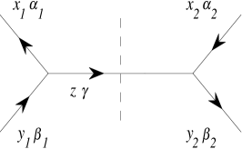
Figure 2: Diagram representing the evolution kernel $K_{\beta_{1}\beta_{2}}^{\alpha_{1}\alpha_{2}}(x_{1},y_{1};x_{2},y_{2})$ at $0<x_{k}<y_{k}$.

In this Appendix we show how the positivity property (7) of the evolution kernel $K_{\beta_{1}\beta_{2}}^{\alpha_{1}\alpha_{2}}(x_{1},x_{2};y_{1},y_{2})$ can be seen in the direct diagrammatic calculation of these kernels. Generally speaking, the leading order evolution kernel gets contributions from several diagrams BFKL-85 but in the region $0<x_{k}<y_{k}$ (6) which is interesting for us this kernel is given by the single cut diagram of Fig. 2. This diagram leads to the following structure of the evolution kernel

$$K_{\beta_{1}\beta_{2}}^{\alpha_{1}\alpha_{2}}(x_{1},x_{2};y_{1},y_{2})=\sum\limits_{\gamma}\delta(y_{1}-x_{1}-y_{2}+x_{2})$$

$$\times V_{\alpha_{1}\beta_{1}\gamma}(x_{1},y_{1})V_{\alpha_{2}\beta_{2}\gamma}^{\ast}(x_{2},y_{2})\,.$$ (29)

In the framework of Ref. BFKL-85 this contribution naturally appears from the pole integration over the light-like component of the momentum. In the case $x_{1},x_{2}>0$ the poles of the propagators associated with $x_{1}$ and $x_{2}$ lie on the same side of the real axis. Shifting the integration contour to the opposite side one can get a nonzero contribution only from the pole of the propagator corresponding to the intermediate parton in the diagram of Fig. 2. Functions $V_{\alpha_{k}\beta_{k}\gamma}(x_{k},y_{k})$ correspond to the two vertices of the diagram of Fig. 2. The kinematical and normalization factors associated with the cut propagator are obviously positive (this positivity is explicit in the light-cone gauge) and can be included into factors $V_{\alpha_{k}\beta_{k}\gamma}(x_{k},y_{k})$. In the RHS of Eq. (29) one sums over the polarization $\gamma$ of the intermediate parton. Using the light-cone gauge and the techniques of Ref. BFKL-85 it is easy to see that the summation over $\gamma$ is restricted to the physical polarizations of the intermediate parton. Note that we can rewrite (29) in the form

$$K_{\beta_{1}\beta_{2}}^{\alpha_{1}\alpha_{2}}(x_{1},x_{2};y_{1},y_{2})$$

$$=\int\limits_{0}^{\infty}dz\sum\limits_{\gamma}W_{\alpha_{1}\beta_{1}\gamma,z}(x_{1},y_{1})W_{\alpha_{2}\beta_{2}\gamma,z}^{\ast}(x_{2},y_{2})$$ (30)

where

$$W_{\alpha\beta\gamma,z}(x,y)=\delta(y-x-z)V_{\alpha\beta\gamma}(x,y)\,.$$ (31)

Obviously the form (30) of the evolution kernel $K$ automatically leads to the positivity property (7). Actually the general decomposition (30) is essentially equivalent to the inequality (7). It is decomposition (30) that is needed for the proof of the stability of the positivity bounds on GPDs with respect to the evolution to higher normalization points.

In order to illustrate the above general formulas with an explicit example let us consider the evolution kernel for the “helicity-independent” quark GPDs

$$\sum\limits_{\alpha}K^{\alpha\alpha}_{\beta_{1}\beta_{2}}(x_{1},x_{2};y_{1},y_{2})\equiv\delta_{\beta_{1}\beta_{2}}K(x_{1},x_{2};y_{1},y_{2})\,.$$ (32)

In the region (6), $0<x_{k}<y_{k}$, the kernel $K$ is given by the following expression BFKL-85

$$K(x_{1},x_{2};y_{1},y_{2})=\frac{C_{F}}{2\pi^{2}}$$

$$\times\frac{\delta(y_{1}-x_{1}-y_{2}+x_{2})}{y_{1}-x_{1}}\left(1+\frac{x_{1}x_{2}}{y_{1}y_{2}}\right)\,.$$ (33)

Obviously this kernel has the form (29)

$$K(x_{1},x_{2};y_{1},y_{2})=\frac{C_{F}}{2\pi^{2}}\delta(y_{1}-x_{1}-y_{2}+x_{2})$$

$$\times\left(\frac{1}{\sqrt{y_{1}-x_{1}}}\frac{1}{\sqrt{y_{2}-x_{2}}}+\frac{x_{1}}{y_{1}\sqrt{y_{1}-x_{1}}}\frac{x_{2}}{y_{2}\sqrt{y_{2}-x_{2}}}\right)\,.$$ (34)

This contribution comes from the diagram of Fig. 2 with a gluon playing the role of the intermediate parton. The two terms in the brackets in the RHS correspond to two possible polarizations of this gluon.

The above expression for the kernel $K$ is singular at the points $y_{k}=x_{k}$. The proper treatment of these singularities is described by the following expression for the convolution of the kernel $K$ with arbitrary functions $h(x,y)$ Ji-97 ; Radyushkin-97 ; BM-98

$$\int\limits_{0}^{\infty}dx_{1}\int\limits_{x_{1}}^{\infty}dy_{1}\int\limits_{0}^{\infty}dx_{2}\int\limits_{x_{2}}^{\infty}dy_{2}h(x_{1},y_{1})h^{\ast}(x_{1},y_{1})$$

$$\times K(x_{1},x_{2};y_{1},y_{2})=\frac{C_{F}}{2\pi^{2}}\lim_{\varepsilon\rightarrow 0}\int\limits_{0}^{\infty}dx_{1}\int\limits_{0}^{\infty}dx_{2}\left\{\int\limits_{\varepsilon}^{\infty}\frac{dz}{z}\right.$$

$$\times\left[1+\frac{x_{1}x_{2}}{(x_{1}+z)(x_{2}+z)}\right]h(x_{1},x_{1}+z)h^{\ast}(x_{2},x_{2}+z)$$

$$\left.+\left(\frac{3}{2}-\ln\frac{4x_{1}x_{2}}{\varepsilon^{2}}\right)h(x_{1},x_{1})h^{\ast}(x_{2},x_{2})\right\}\,.$$ (35)

The last term in the RHS proportional to $h(x_{1},x_{1})h^{\ast}(x_{2},x_{2})$ corresponds to the virtual $\delta(y_{1}-x_{1})\delta(y_{2}-x_{2})$ contributions to the evolution kernel $K$. In the limit $\varepsilon\rightarrow 0$ both integral and contact terms are divergent but these two divergences cancel each other.

Appendix B Stability of positivity bounds under evolution

In this Appendix we present a detailed derivation of the stability of the positivity bounds (3) under the one-loop evolution (5) to higher normalization points. We shall use compact Dirac notation for the integral appearing in the LHS of inequality (3)

$$\langle f|G|f\rangle\equiv\sum\limits_{i_{1}\alpha_{1}i_{2}\alpha_{2}}\int\frac{dP_{1}^{+}d^{2}P_{1}^{\perp}dx_{1}}{2P_{1}^{+}(2\pi)^{3}}\int\frac{dP_{2}^{+}d^{2}P_{2}^{\perp}dx_{2}}{2P_{2}^{+}(2\pi)^{3}}$$

$$\times\theta(x_{1})\theta(x_{2})\,f_{i_{2}\alpha_{2}}^{\ast}(x_{2},P_{2})f_{i_{1}\alpha_{1}}(x_{1},P_{1})G_{P_{1}i_{1},P_{2}i_{2}}^{\alpha_{1}\alpha_{2}}(x_{1},x_{2})$$ (36)

so that the positivity bound (3) can be written as follows

$$\langle f|G|f\rangle\geq 0\,.$$ (37)

Let us assume that at some normalization point inequality (3) holds for all functions $f_{i\alpha}(x,P)$. Imagine that during the evolution to higher $\mu$ this inequality breaks down at some point $\mu_{0}$ for some function $f^{(0)}$ so that at $\mu>\mu_{0}$

$$\langle f^{(0)}|G_{\mu}|f^{(0)}\rangle<0\quad(\mu>\mu_{0})$$ (38)

but at $\mu<\mu_{0}$ we still have for all functions $f$

$$\langle f|G_{\mu}|f\rangle\geq 0\quad(\mu\leq\mu_{0})\,.$$ (39)

Then at point $\mu_{0}$

$$\langle f^{(0)}|G_{\mu_{0}}|f^{(0)}\rangle=0\,.$$ (40)

The fate of this “matrix element” at $\mu>\mu_{0}$ is determined by the evolution equation (5)

$$\mu\frac{\partial}{\partial\mu}\langle f^{(0)}|G_{\mu}|f^{(0)}\rangle=\langle f^{(0)}|(K\otimes G_{\mu})|f^{(0)}\rangle\,.$$ (41)

Here we use short notation $K\otimes G_{\mu}$ for the convolution of the evolution kernel $K$ with GPD $G$. If one could show that at the point $\mu_{0}$ we have

$$\langle f^{(0)}|(K\otimes G_{\mu_{0}})|f^{(0)}\rangle\geq 0$$ (42)

then this would guarantee that the evolution from $\mu_{0}$ to higher $\mu$ would restore the positivity of $\langle f^{(0)}|G_{\mu}|f^{(0)}\rangle$. This would invalidate our assumption (38). Thus in order to prove the stability of the positivity bounds on GPD under the evolution to higher normalization points we need the following

Statement. If at some normalization point $\mu_{0}$ for all functions $f$

$$\langle f|G_{\mu_{0}}|f\rangle\geq 0$$ (43)

and for some $f^{(0)}$

$$\langle f^{(0)}|G_{\mu_{0}}|f^{(0)}\rangle=0$$ (44)

then

$$\langle f^{(0)}|(K\otimes G_{\mu_{0}})|f^{(0)}\rangle\geq 0\,.$$ (45)

To prove this statement we make use of the positivity property of the evolution kernels (7). As it is explained in Appendix A this positivity property is equivalent to the decomposition (30) of the evolution kernel. In our short Dirac-like notations Eq. (30) takes the following form

$$K=\int dz\sum\limits_{\gamma}|W_{\gamma,z}\rangle\langle W_{\gamma,z}|$$ (46)

Inserting representation (46) for $K$ into the LHS of inequality (45) we find

$$\langle f^{(0)}|(K\otimes G_{\mu_{0}})|f^{(0)}\rangle$$

$$=\int dz\sum\limits_{\gamma}\langle f^{(0)}\otimes W_{\gamma,z}|G_{\mu_{0}}|f^{(0)}\otimes W_{\gamma,z}\rangle\geq 0\,.$$ (47)

The RHS is positive according to Eq. (43). This completes the derivation of the inequality (45).

The above proof of the stability of the positivity bounds (3) under the evolution (5) ignored the problem of the negative terms proportional to $\delta(x_{1}-y_{1})\delta(x_{2}-y_{2})$ which are present in the evolution kernel $K$. Because of these terms it is allowed to use inequality (7) only for functions $h(x,y)$ which vanish at $x=y$. As a result instead of Eq. (46) one has to work with the following representation for the evolution kernel

$$K=\lim_{\varepsilon\rightarrow+0}\left(K_{\varepsilon}^{(1)}+K_{\varepsilon}^{(2)}\right)$$ (48)

where the first term is given by the $\varepsilon$ regularized integral decomposition (46)

$$K_{\varepsilon}^{(1)}(x_{1},x_{2},y_{1},y_{2})=\int\limits_{\varepsilon}^{\infty}dz\sum\limits_{\gamma}W_{\gamma,z}(x_{1},y_{1})W_{\gamma,z}^{\ast}(x_{2},y_{2})$$ (49)

and the second piece

$$K_{\varepsilon}^{(2)}(x_{1},x_{2},y_{1},y_{2})=C(\varepsilon,x_{1},x_{2})\delta(x_{1}-y_{1})\delta(x_{2}-y_{2})$$ (50)

comes from the virtual contribution to the evolution kernel which is proportional to $\delta(x_{1}-y_{1})\delta(x_{2}-y_{2})$ with a divergent coefficient $C(\varepsilon,x_{1},x_{2})$. This coefficient is regularized by the same small parameter $\varepsilon$ so that

$$C(\varepsilon,x_{1},x_{2})=c_{1}+c_{2}\ln\varepsilon+F_{1}(x_{1})+F_{2}(x_{2})\,.$$ (51)

The singular contribution $\ln\varepsilon$ compensates the divergence of the $z$ integral in the RHS of Eq. (49). Obviously representation (48) guarantees that $K$ obeys inequality (7) for arbitrary functions $h(x,y)$ vanishing at $x=y$. An example of the general structure (51) can be seen in the explicit expression (35) for the quark evolution kernel where the term $\ln((4x_{1}x_{2})/\varepsilon^{2})$ represents all terms appearing in the rhs of (51).

Now we have to show that the kernel $K$ (48) still has the property (45). For the first term in the RHS of Eq. (48) this can be done in the same way as in the inequality (47):

$$\langle f^{(0)}|(K_{\varepsilon}^{(1)}\otimes G_{\mu_{0}})|f^{(0)}\rangle\geq 0\,.$$ (52)

Next let us show that

$$\langle f^{(0)}|(K_{\varepsilon}^{(2)}\otimes G_{\mu_{0}})|f^{(0)}\rangle=0\,.$$ (53)

According to Eqs. (50), (51) we have

$$\langle f^{(0)}|(K_{\varepsilon}^{(2)}\otimes G_{\mu_{0}})|f^{(0)}\rangle=\langle f^{(0)}|[(c_{1}+c_{2}\ln\varepsilon)G_{\mu_{0}}$$

$$+G_{\mu_{0}}F_{1}+F_{2}G_{\mu_{0}}]|f^{(0)}\rangle\,.$$ (54)

Note that $|f^{(0)}\rangle$ is associated with $f^{(0)}(x_{1},y_{1})$ whereas $\langle f^{(0)}|$ corresponds to $f^{(0)}(x_{2},y_{2})$ in Eq. (36). This explains the ordering of “operators” $F_{1}$ and $F_{2}$ associated with functions $F_{1}(x_{1})$ and $F_{2}(x_{2})$ respectively in the RHS of Eq. (54). Taking into account Eq. (44) we get rid of the $c_{1}+c_{2}\ln\varepsilon$ contribution:

$$\langle f^{(0)}|(K_{\varepsilon}^{(2)}\otimes G_{\mu_{0}})|f^{(0)}\rangle$$

$$=\langle f^{(0)}|(G_{\mu_{0}}F_{1}+F_{2}G_{\mu_{0}})|f^{(0)}\rangle\,.$$ (55)

Since property of $G_{\mu_{0}}$ (43) holds for any $f$ we conclude from Eq. (44) that

$$G_{\mu_{0}}|f^{(0)}\rangle=0\,,\quad\langle f^{(0)}|G_{\mu_{0}}=0\,.$$ (56)

This means that

$$\langle f^{(0)}|(G_{\mu_{0}}F_{1}+F_{2}G_{\mu_{0}})|f^{(0)}\rangle=0\,.$$ (57)

Inserting this result into Eq. (55) we obtain Eq. (53). Combining Eqs. (52), (53) we derive inequality (45), which means that the virtual terms in the evolution kernel do not violate the stability of the positivity bounds on parton distributions under the evolution to higher normalization points.

Appendix C Derivation of positivity bounds in impact parameter representation

In this Appendix we show how inequality (3) containing a multidimensional integral can be reduced to the relatively simple form (11).

Using representation (8) for GPD $G$ we find from inequality (3)

$$\int\limits_{0}^{\infty}dk^{+}_{1}\int\limits_{0}^{\infty}\frac{dP_{1}^{+}}{P_{1}^{+}}\int d^{2}P_{1}^{\perp}\,\int\limits_{0}^{\infty}dk^{+}_{2}\int\limits_{0}^{\infty}\frac{dP_{2}^{+}}{P_{2}^{+}}\int d^{2}P_{2}^{\perp}$$

$$\times\delta\left[(P_{2}^{+}-k^{+}_{2})-(P_{1}^{+}-k^{+}_{1})\right]$$

$$\times F_{\sigma_{2}\sigma_{1}}\left[\frac{k^{+}_{1}+k^{+}_{2}}{P_{1}^{+}+P_{2}^{+}},\frac{P_{1}^{+}-P_{2}^{+}}{P_{1}^{+}+P_{2}^{+}},\frac{2(P_{1}^{+}P_{2}^{\perp}-P_{2}^{+}P_{1}^{\perp})}{P_{1}^{+}+P_{2}^{+}}\right]$$

$$\times f_{\sigma_{2}}^{\ast}(k^{+}_{2},P_{2}^{+},P_{2}^{\perp})f_{\sigma_{1}}(k^{+}_{1},P_{1}^{+},P_{1}^{\perp})\geq 0\,.$$ (58)

Taking functions $f_{\sigma}$ in the factorized form

$$f_{\sigma}(k^{+},P^{+},P^{\perp})=d_{\sigma}(k^{+},P^{+})\eta\left(\frac{P^{\perp}}{P^{+}}\right)$$ (59)

we derive from inequality (58)

$$\int\limits_{0}^{\infty}dk^{+}_{1}\int\limits_{0}^{\infty}dP_{1}^{+}\int\limits_{0}^{\infty}dk^{+}_{2}\int\limits_{0}^{\infty}dP_{2}^{+}d_{\sigma_{2}}^{\ast}(k^{+}_{2},P_{2}^{+})d_{\sigma_{1}}(k^{+}_{1},P_{1}^{+})$$

$$\times\tilde{F}_{\sigma_{2}\sigma_{1}}\left[\frac{k^{+}_{1}+k^{+}_{2}}{P_{1}^{+}+P_{2}^{+}},\frac{P_{1}^{+}-P_{2}^{+}}{P_{1}^{+}+P_{2}^{+}},\frac{P_{1}^{+}+P_{2}^{+}}{2P_{1}^{+}P_{2}^{+}}b^{\perp}\right]$$

$$\times\delta\left[(P_{2}^{+}-k^{+}_{2})-(P_{1}^{+}-k^{+}_{1})\right]\left(\frac{P_{1}^{+}+P_{2}^{+}}{2P_{1}^{+}P_{2}^{+}}\right)^{2}\geq 0$$ (60)

where $\tilde{F}_{\sigma_{2}\sigma_{1}}$ is defined by Eq. (10). This inequality should hold for any value of $b^{\perp}$ and for any function $d_{\sigma}(k^{+},P^{+})$. The next step is to take

$$d_{\sigma}(k^{+},P^{+})=g(P^{+}-k^{+})h_{\sigma}(P^{+})\,.$$ (61)

In the limit

$$\left|g(u)\right|^{2}\rightarrow\delta(u-\nu)$$ (62)

we find from inequality (60)

$$\int\limits_{-1}^{1}d\xi\int\limits_{|\xi|}^{1}dx\frac{1}{(1-x)(1-\xi^{2})^{2}}h_{\sigma_{2}}^{\ast}\left(\nu\frac{1-\xi}{1-x}\right)$$

$$\times h_{\sigma_{1}}\left(\nu\frac{1+\xi}{1-x}\right)\tilde{F}_{\sigma_{2}\sigma_{1}}\left(x,\xi,\frac{(1-x)b^{\perp}}{\nu(1-\xi^{2})}\right)\geq 0\,.$$ (63)

Since function $h_{\sigma}$ and parameter $b^{\perp}$ are arbitrary we can set $\nu=1$ without losing generality. Taking $h_{\sigma}(z)=z^{2}p_{\sigma}(z^{-1})$ we obtain inequality (11).

References

• (1) D. Müller, D. Robaschik, B. Geyer, F.-M. Dittes, and J. Hořejši, Fortschr. Phys. 42 (1994) 101.
• (2) A.V. Radyushkin, Phys. Lett. B385 (1996) 333.
• (3) X. Ji, Phys. Rev. Lett. 78 (1997) 610; Phys. Rev. D55 (1997) 7114.
• (4) J.C. Collins, L. Frankfurt, and M. Strikman, Phys. Rev. D56 (1997) 2982.
• (5) A.V. Radyushkin, Phys. Rev. D56 (1997) 5524.
• (6) A.V. Radyushkin, in Shifman M. (ed.): At the frontier of particle physics, vol. 2, pp. 1037-1099 (World Scientific, Singapore, 2001).
• (7) K. Goeke, M.V. Polyakov and M. Vanderhaeghen, Prog. Part. Nucl. Phys.  47 (2001) 401.
• (8) A.V. Belitsky, D. Müller and A. Kirchner, Nucl. Phys. B629 (2002) 323.
• (9) A.D. Martin and M.G. Ryskin, Phys. Rev. D57 (1998) 6692.
• (10) A.V. Radyushkin, Phys. Rev. D59 (1999) 014030.
• (11) B. Pire, J. Soffer, and O. Teryaev, Eur. Phys. J. C8 (1999) 103.
• (12) X. Ji, J. Phys. G24 (1998) 1181.
• (13) M. Diehl, T. Feldmann, R. Jakob, and P. Kroll, Nucl. Phys. B596 (2001) 33.
• (14) M. Burkardt, hep-ph/0105324.
• (15) P.V. Pobylitsa, Phys. Rev. D65 (2002) 077504.
• (16) P.V. Pobylitsa, Phys. Rev. D65 (2002) 114015.
• (17) M. Diehl, hep-ph/0205208.
• (18) M. Burkardt, hep-ph/0206269.
• (19) M. Burkardt, hep-ph/0207047.
• (20) V.N. Gribov and L.N. Lipatov, Sov. J. Nucl. Phys. 15 (1972) 438;
L.N. Lipatov, Sov. J. Nucl. Phys. 20 (1974) 94;
A.P. Bukhvostov, L.N. Lipatov and N.P. Popov, Sov. J. Nucl. Phys. 20 (1974) 287.
• (21) G. Altarelli and G. Parisi, Nucl. Phys. B126 (1977) 298.
• (22) Yu.L. Dokshitzer, Sov. Phys. JETP 46 (1977) 641.
• (23) G. Altarelli, S. Forte, G. Ridolfi, Nucl. Phys. B534 (1998) 277.
• (24) A.P. Bukhvostov, G.V. Frolov, L.N. Lipatov and E.A. Kuraev, Nucl. Phys. B258 (1985) 601.
• (25) A.V. Belitsky, D. Müller, Nucl. Phys. B527 (1998) 207.