Transport Coefficients and Ladder Summation
in Hot Gauge Theories

Abstract

We show how to compute transport coefficients in gauge theories by considering the expansion of the Kubo formulas in terms of ladder diagrams in the imaginary time formalism. All summations over Matsubara frequencies are performed and the analytical continuation to get the retarded correlators is done. As an illustration of the procedure, we present a derivation of the transport equation for the shear viscosity in the scalar theory. Assuming the Hard Thermal Loop approximation for the screening of distant collisions of the hard particles in the plasma, we derive a couple of integral equations for the effective vertices which, to logarithmic accuracy, are shown to be identical to the linearized Boltzmann equations previously found by Arnold, Moore and Yaffe.

I Introduction

The development of a transport theory for QCD in the regime of high temperature has turned out a valuable pursuit with the advent of heavy ion colliders which provide novel tools for the study of the properties of highly excited matter. From a purely theoretical point of view, the computation of transport coefficients amounts a challenge even in weakly coupled theories, because these quantities usually depend non-analytically on the coupling constant. In most previous computations Baym ; Heiselberg ; Baym2 , a kinetic approach based in the Boltzmann equation has been used. It is only recently within this framework that a reliable computation to logarithmic accuracy in gauge theories has been reported Arnold1 . The complete leading order is still unavailable except for the case of a gauge theory with a large number of fermionic species Moore .

However, there exists an alternative approach based on Kubo formulas for appropriate correlation functions, which has been largely used in the context of low energy many-body physics Mahan . For the electrical and thermal conductivities of ordinary metals and superconductors, the computation of the current correlators requires the resummation of an infinite class of ladder diagrams, a task that in the complete relativistic setting of gauge theories usually appears as a very hard issue, partly motivating the scant of this approach. In relativistic transport theory, the resummation of ladder diagrams has been performed for the scalar theory by Jeon Jeon , who proved the equivalence with the Boltzmann equation, and since repeated a few times Carrington ; Wang . Also, a simplified ladder summation has been performed for the computation of the leading-log order of the color conductivity Martinez . Recently, Arnold, Moore and Yaffe Arnold2 ; Arnold3 have performed a ladder summation in order to account for the effect of multiple scattering in the process of photon production from a QCD plasma.

The purpose of this paper is twofold. First, we wish to explicitly show how to perform the summation of a restricted set of ladder diagrams in gauge theories within the imaginary time formalism of thermal field theory. In contrast to the work of Jeon Jeon , we will not use the series of cut ladder diagrams. Rather, we closely follow a treatment due to Holstein Holstein who, a long time ago, performed a ladder summation in order to compute the transport properties of the low-energy electron-phonon gas. In this approach, one first identifies the required analytic continuation of the effective vertex function entering in the current correlator, and then writes the integral equation for this vertex, summing all ladders. As shown below, this approach exactly reproduces the correct transport equation for the shear viscosity in the scalar theory.

On the other hand, we will try to derive the logarithmic accuracy of the transport coefficients by only considering the role played by the soft degrees of freedom which are exchanged in the collisions between the plasma constituents. This requires the use of the Hard Thermal Loop (HTL) approximation HTL for the internal lines associated with the rungs of the diagrams, and the introduction of an arbitrary momentum scale $q_{c}$ separating the hard and soft ranges of the momentum transfer Yuan . An important step towards the complete computation of the hard contribution was already recently made by the authors of Ref. Arnold1 , who calculated the infrared logarithmic divergences of the collision terms of linearized Boltzmann equation written in terms of unscreened interactions.

Our main results are a couple of integral equations for the effective vertices, encoding the effects of distant collisions in the plasma coming from soft momentum transfer $q<q_{c}$. Although these equations are necessarily incomplete, they reproduce the required logarithmic dependence on $q_{c}$ which makes possible the eventual cancellation of the arbitrary scale $q_{c}$ in the final result. Hence, they reproduce the known results Arnold1 for the transport coefficients to logarithmic accuracy.

The plan of this paper is as follows. In Sec. II, we review some standard material on the imaginary time formalism of thermal field theory and Kubo formulas. Here, we include a useful summation formula over Matsubara frequencies and the procedure of analytic continuation. In Sec. III we show how to derive the shear viscosity of $\lambda\phi^{4}$ theory. Section IV deals with the simplifications which appear by summing the ladders when only the effect of soft momentum transfer is considered. Then, we derive the corresponding contribution to the transport equations for the electrical conductivity and the shear viscosity. Section V presents a brief derivation based on sum rules of the logarithmic terms in the transport coefficients, and Sec. VI closing the paper contains a summary and prospects. There are short appendixes with some details about spectral densities, sum rules and the relevant thermal widths to be included in the propagators of hard particles.

II Basic formalism

II.1 Single particle spectral densities

The basic element of a diagram in the Imaginary-Time Formalism is the Matsubara propagator depending on the purely imaginary frequencies $i\omega_{n}=i\pi n/\beta$ (with $n$ even for bosons and odd for fermions),

$$\Delta(i\omega_{n},{\mathbf{q}})=\int_{-\infty}^{\infty}\frac{dq^{0}}{2\pi}\frac{\rho(Q)}{q^{0}-i\omega_{n}},$$ (1)

where the real quantity $\rho(Q)$ (with $Q^{\mu}=(q^{0},{\mathbf{q}})$, $q^{0}$ real) is the single particle spectral density. The analytical continuation $i\omega_{n}\rightarrow z$ defines a function $\Delta(z,{\mathbf{q}})$ of a complex variable $z$ which is analytical off the real axis and the discontinuity through the branch cut along $\rm{Im}\,z=0$ is proportional to $\rho(Q)$. The different Green’s functions for real frequency can be constructed from the spectral density. For instance, the bosonic Wightman functions $\Delta^{>,\,<}(Q)$ are given by

$$\Delta^{>}(Q)=\left(1+n_{b}(q^{0})\right)\rho(Q),\qquad\Delta^{<}(Q)=n_{b}(q^{0})\rho(Q),$$ (2)

where $n_{b}(q^{0})=1/(e^{\beta q^{0}}-1)$ is the bosonic occupation number. The retarded and advanced Green’s functions, which will play an important role in our discussion, are

$$\Delta^{\rm{ret}}(Q)=\Delta(q^{0}+i0^{+},{\mathbf{q}}),\qquad\Delta^{\rm{adv}}(Q)=\Delta(q^{0}-i0^{+},{\mathbf{q}}),$$ (3)

and $\rho(Q)=2\,\rm{Im}\,\Delta^{\rm{ret}}(Q)$.

For a free particle, the spectral density is given by a superposition of delta functions, with support on the mass shell, $p_{0}^{2}=\varepsilon_{p}^{2}$. If the interactions are weak, a delta function can be replaced by a Lorentzian with a small width $\Gamma_{p}$, related to the imaginary part of the energy at the poles of the retarded propagator, $p^{0}=\pm\varepsilon_{p}-i\Gamma_{p}$,

$$2\pi\delta(p^{0}\mp\varepsilon_{p})\longmapsto\frac{2\Gamma_{p}}{(p^{0}\mp\varepsilon_{p})^{2}+\Gamma_{p}^{2}},$$ (4)

which gives rise to an analytical propagator

$$\Delta(z,{\mathbf{p}})=\int_{-\infty}^{\infty}\frac{dp^{0}}{2\pi}\frac{2\Gamma_{p}}{(p^{0}\mp\varepsilon_{p})^{2}+\Gamma_{p}^{2}}\,\frac{1}{p^{0}-z}=\frac{-1}{z\mp\varepsilon_{p}+i\Gamma_{p}\,\rm{sign}(\rm{Im}\,z)}.$$ (5)

Thus, for this case, the function $\Delta(z,{\mathbf{p}})$ has a branch cut at real axis in the complex $z$-plane and it has no poles.

At high temperature, the particles entering in the collision processes occurring in the plasma are mostly particles propagating nearly on-shell with hard momentum, $P\sim T$. Their spectral densities may be approximated by a combination of two Lorentzians

$$\rho_{b}(P) = \frac{1}{p}\left(\frac{\Gamma_{p}}{(p^{0}-p)^{2}+\Gamma_{p}^{2}}-\frac{\Gamma_{p}}{(p^{0}+p)^{2}+\Gamma_{p}^{2}}\right),$$ (6)

$$\rho_{f}(P) = \left(\frac{2\gamma_{p}}{(p^{0}-p)^{2}+\gamma_{p}^{2}}h_{+}(\hat{\mathbf{p}})+\frac{2\gamma_{p}}{(p^{0}+p)^{2}+\gamma_{p}^{2}}h_{-}(\hat{\mathbf{p}})\right),$$ (7)

where $h_{\pm}(\hat{\mathbf{p}})=(\gamma^{0}\mp{\bm{\gamma}}\cdot\hat{\mathbf{p}})/2$, and the thermal widths $\Gamma_{p}$ and $\gamma_{p}$ are the imaginary parts of the transverse piece of the on-shell gluon self-energy and the quark, respectively

$$\Gamma_{p} = -\frac{1}{2p}{\rm Im}\,\Pi_{\rm{T}}^{\rm{ret}}(p^{0}=p,\mathbf{p}),$$ (8)

$$\gamma_{p} = -\frac{1}{4p}{\rm{tr}}\left({\hbox to0.0pt{\hbox to5.03125pt{\hfil/\hfil}\hss}p}\,{\rm Im}\,\Sigma^{\rm{ret}}(p^{0}=p,\mathbf{p})\right).$$ (9)

The shift in the real part of the energy can be ignored since it is perturbatively small when the energy is $O(T)$.

In gauge theories, the imaginary part of the thermal self-energies receives contributions from various scattering processes which give a different dependence on the coupling constant. Generically, two body scattering processes in which a soft bosonic excitation is exchanged yield a parametric dependence at leading order as $\Gamma_{p},\gamma_{p}\propto g^{2}T\log(\Lambda_{\rm{max}}/\Lambda_{\rm{min}})$, whereas processes in which a soft fermionic excitation is exchanged yield a parametric dependence $\Gamma_{p},\gamma_{p}\propto g^{4}T^{2}\log(q_{c}/gT)/p$. The cutoff $q_{c}$ is a scale separating semihard and hard momentum transfers, restricted by $gT\ll q_{c}\ll T$ but otherwise arbitrary, and $\Lambda_{\rm{max}}$ can be chosen of order $gT$. As will be explicitly showed below, the infrared sensitivity to the lower cutoff $\Lambda_{\rm{min}}\sim g^{2}T$ entirely disappears from the transport coefficients to be computed.

On the other hand, the temperature Green’s functions for the soft bosonic and fermionic excitations are determined by the single particle spectral densities in the hard thermal loop approximation, ${}^{\ast}\rho_{\rm{L,T}}(\omega,{\mathbf{q}})$ and ${}^{\ast}\Delta_{\pm}(\omega,{\mathbf{q}})$, respectively HTL ; Blaizot ; Lebellac . These are presented in the appendices B and C. Already, let us note here that only the Landau damping piece of these will contribute to the screening of distant collisions.

II.2 Kubo formulas and the ladder approximation

Our starting point is the Kubo formula expressing a given transport coefficient in terms of the low frequency, zero momentum limit of the spectral density for the corresponding correlation function. For the electrical conductivity and the shear viscosity the formulas are Mahan ; Jeon

$$\sigma = \frac{1}{6}\lim_{\omega\rightarrow 0}\,\lim_{{\mathbf{q}}\rightarrow 0}\frac{\partial}{\partial\omega}\rho_{JJ}(\omega,{\mathbf{q}}),$$ (10)

$$\eta = \frac{1}{20}\lim_{\omega\rightarrow 0}\,\lim_{{\mathbf{q}}\rightarrow 0}\frac{\partial}{\partial\omega}\rho_{\pi\pi}(\omega,{\mathbf{q}}),$$ (11)

where, as usual, the spectral densities are related to the Fourier transform of the retarded correlators by

$$\rho_{JJ}(\omega,{\mathbf{q}}) = 2\,{\rm Im}\int_{-\infty}^{\infty}dt\int d^{3}x\,e^{i\omega t-i{\mathbf{q}}\cdot{\mathbf{x}}}\langle\left[J_{i}(t,{\mathbf{x}}),J_{k}(0)\right]\rangle\theta(t)\delta_{ik},$$ (12)

$$\rho_{\pi\pi}(\omega,{\mathbf{q}}) = 2\,{\rm Im}\int_{-\infty}^{\infty}dt\int d^{3}x\,e^{i\omega t-i{\mathbf{q}}\cdot{\mathbf{x}}}\langle\left[\pi_{ij}(t,{\mathbf{x}}),\pi_{ij}(0)\right]\rangle\theta(t),$$ (13)

and the averages are evaluated in the equilibrium grand canonical ensemble. An efficient way to compute a retarded correlator $\Pi_{AA}^{\rm{ret}}(\omega,{\mathbf{q}})$ (with $A$ denoting collectively the indices of the appropriate current) is to exploit the spectral representation for complex frequency $z$. This provides a direct connection with the temperature Green’s function $\Pi_{AA}(i\nu_{n},{\mathbf{q}})$, via analytic continuation $i\nu_{n}\rightarrow\omega+i0^{+}$. Thus, a first step in our basic task is to evaluate $\Pi_{AA}(i\nu_{n},{\mathbf{0}})$ within the imaginary time formalism.

After the laborious diagrammatic analysis explicitly performed for the scalar theory Jeon , the conclusion is that, in order to account for all leading-order contributions to the shear viscosity, a set of uncrossed ladder diagrams must be summed. On the other hand, for the processes of photon production from a QCD plasma, the authors of Refs. Arnold2 ; Arnold3 have developed detailed power counting arguments which enforce the resummation of the uncrossed ladder graphs made of gauge boson rungs.

A key point for understand the equal footing of this class of diagrams is the presence of pairs of propagators carrying nearly the same momenta, which leads to a dependence $1/\Gamma_{p}$ (or $1/\gamma_{p}$) by each such a propagator pair. Hence, it is clear that a $(n+1)$-loop diagram with $n$ uncrossed rungs leads to a dependence proportional to $\alpha^{2}(1/\Gamma_{p})^{n+1}(g^{2})^{n}$, where the first $\alpha^{2}$ comes from the two external insertions, and each rung introduces a factor $g^{2}$. The derived result in both cases Jeon and Arnold2 is a linear integral equation for an effective vertex function, which is completely equivalent to the linearized transport equation for the problem. Here, we will proceed by assuming the dominance of the same set of ladder diagrams, relying on a posteriori check of its consistency.

At this point, let us then to introduce an amputated effective vertex $\Lambda_{A}(i\omega_{m}+i\nu_{n},i\omega_{m};{\mathbf{p}})$, associated with two hard external bosonic or fermionic lines $(i\omega_{m}+i\nu_{n},{\mathbf{p}})$ , $(i\omega_{m},{\mathbf{p}})$ and with an insertion of zero external momentum but non-zero frequency $(i\nu_{n},{\mathbf{0}})$, corresponding to the appropriate current ($J_{i}$ or $\pi_{ij}$). This effective vertex (Fig. 1) is the sum of all vertices, each one of them with a number $n$ of rungs associated with the exchanged excitations, and presumably will encode all collision effects at leading order. The vertex having zero rungs, $\Lambda_{A}^{(0)}({\mathbf{p}})$, does not depend on the frequencies but can depend on the momentum ${\mathbf{p}}$.

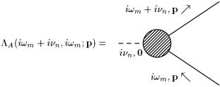
Figure 1: Labels of the effective vertex.

II.3 Summation over Matsubara frequencies and analytic continuation

Let us now to examine the summation over Matsubara frequencies, which generically is involved in the evaluation of a temperature correlator $\Pi_{AA}(i\nu_{n},{\mathbf{0}})$,

$$T\sum_{\omega_{m}}G(i\omega_{m}+i\nu_{n},{\mathbf{p}})\Lambda_{A}(i\omega_{m}+i\nu_{n},i\omega_{m};{\mathbf{p}})G(i\omega_{m},{\mathbf{p}})\Lambda_{A}^{(0)}({\mathbf{p}}),$$ (14)

where the Matsubara propagators have spectral densities of the form (6) or (7).

To one-loop order, the effective vertex reduces to $\Lambda_{A}^{(0)}$ and the above sum over frequencies becomes

$$H(i\nu_{n},{\mathbf{p}})=T\sum_{\omega_{m}}G(i\omega_{m}+i\nu_{n},{\mathbf{p}})G(i\omega_{m},{\mathbf{p}}),$$ (15)

with $\nu_{n}$ even in any case. Now, the function to be summed is a product of Green’s functions and one may proceed by expressing the Green’s functions in terms of their spectral representations given by Eq. (1). With this replacement, the resulting expression involves a double frequency integral of the product resulting of the spectral densities and the elementary sum

$$T\sum_{\rm{even,\,odd}\,m}\frac{1}{i\omega_{m}-\omega_{1}}\frac{1}{i\omega_{m}+i\nu_{n}-\omega_{2}}=\mp\,\frac{n_{b,f}(\omega_{1})-n_{b,f}(\omega_{2})}{i\nu_{n}+\omega_{1}-\omega_{2}},$$ (16)

where $n_{b,f}$ denote boson or fermion occupation factors. However, it is more convenient to use an alternative procedure based on contour integration in the $z$-plane of an appropriate function.

This procedure was used, a long time ago, by Holstein Holstein for to derive diagrammatically the transport properties of an electron-phonon gas. Here, we closely follow the treatment of Holstein. To perform the summation (15), we consider the function $G(z+i\nu_{n},{\mathbf{p}})G(z,{\mathbf{p}})n_{b,f}(z)$, and a contour integration $C_{0}$ made of three circuits enclosing the poles of $n_{b,f}(z)$ at the imaginary axis but avoiding the other possible poles of $GG$ (in this case there are absent), and the two branch cuts at ${\rm Im}\,z=0$ and ${\rm Im}(z+i\nu_{n})=0$. This contour may be deformed to $C$ and $\Gamma$ as shown in Fig. 2. The contributions from the large arcs $\Gamma$ vanish and we are left with the integrals along $C$. Then, Eq. (15) becomes after summation

$$H(i\nu_{n},{\mathbf{p}}) = \pm\frac{1}{2\pi i}\int_{C}dz\,G(z+i\nu_{n},{\mathbf{p}})G(z,{\mathbf{p}})n_{b,f}(z)$$ (17)

$$= \mp\int_{-\infty}^{\infty}\frac{d\xi}{2\pi i}n_{b,f}(\xi)\,\left\{\left[G(i\nu_{n}+\xi,{\mathbf{p}})+G(-i\nu_{n}+\xi,{\mathbf{p}})\right]G^{\rm adv}(\xi,{\mathbf{p}})\right.$$

$$-\left.G^{\rm ret}(\xi,{\mathbf{p}})\left[G(i\nu_{n}+\xi,{\mathbf{p}})+G(-i\nu_{n}+\xi,{\mathbf{p}})\right]\right\}$$

where $\xi$ is a variable specifying the position at the branch cuts. More generally, if the function $F(z)$ to be summed has poles in the complex $z$-plane, the summation formula which will be extensively used in what follows is

$$T\sum_{{\rm even,\,odd}\,m}F(i\omega_{m})=\mp\sum_{\rm poles}n_{b,f}(z_{i}){\rm Res}(F,z=z_{i})\pm\sum_{\rm cuts}\int_{-\infty}^{\infty}\frac{d\xi}{2\pi i}n_{b,f}(\xi){\rm Disc}F.$$ (18)

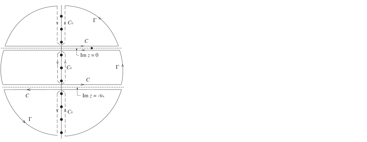
Figure 2: Integration contour for the sum $T\sum_{m}F(i\omega_{m})$. The original contour $C_{0}$ consists of three dashed circuits encircling the Matsubara frequencies. The deformed contour $C$ goes along both sides of the branch cuts. A possible pole of $F(z)$ at the real axis is depicted for its relevance in the summation of the vertex equation.

Application of this formula to the summation in Eq. (14) requires the determination of the singularities of $\Lambda_{A}(z+i\nu_{n},z;{\mathbf{p}})$. We argue that the only singularities are two branch cuts at the lines ${\rm Im}(z+i\nu_{n})=0$ and ${\rm Im}(z)=0$. This is a consequence of the recurrence relation for the vertex with $n$ rungs,

$$\Lambda_{A}^{(n)}(i\omega_{m}+i\nu_{n},i\omega_{m};{\mathbf{p}})=T\sum_{\nu_{q}}\int\frac{d^{4}Q}{(2\pi)^{4}}\,G(i\omega_{m}+i\nu_{n}+i\nu_{q},{\mathbf{p}}+{\mathbf{q}})$$

$$\qquad\times\Lambda_{A}^{(n-1)}(i\omega_{m}+i\nu_{n}+i\nu_{q},i\omega_{m}+i\nu_{q};{\mathbf{p}}+{\mathbf{q}})G(i\omega_{m}+i\nu_{q},{\mathbf{p}}+{\mathbf{q}})\frac{\rho(Q)}{q^{0}-i\nu_{q}}\,,$$ (19)

where $\rho(Q)$ is the spectral density corresponding to the added rung and $(i\nu_{q},{\mathbf{q}})$ label the momenta running through the loop. For $n=1$, it is clear that Eq. (18) implies that $\Lambda_{A}^{(1)}$ has only the singularities of the product of the Green’s functions. Then, it follows from mathematical induction that $\Lambda_{A}^{(n)}$, and hence $\Lambda_{A}$, inherits the same property.

Now, we are ready to perform the summation in Eq. (14) and the subsequent analytic continuation. Making use of Eq. (18) we may write

$$T\sum_{\omega_{m}}G(i\omega_{m}+i\nu_{n})\Lambda_{A}(i\omega_{m}+i\nu_{n},i\omega_{m})G(i\omega_{m})=\mp\int_{-\infty}^{\infty}\frac{d\xi}{2\pi i}n_{b,f}(\xi)$$

$$\quad\times\left\{\left[G(\xi+i\nu_{n})\Lambda_{A}(\xi+i\nu_{n},\xi-i0^{+})+G(\xi-i\nu_{n})\Lambda_{A}(\xi-i0^{+},\xi-i\nu_{n})\right]G^{\rm adv}(\xi)\right.$$

$$\quad-\left.G^{\rm ret}(\xi)\left[\Lambda_{A}(\xi+i\nu_{n},\xi+i0^{+})G(\xi+i\nu_{n})+\Lambda_{A}(\xi+i0^{+},\xi-i\nu_{n})G(\xi-i\nu_{n})\right]\right\},$$ (20)

where the dependence on $\mathbf{p}$ is not explicitly exhibited. Next, the analytical continuation $i\nu_{n}\rightarrow\omega+i0^{+}$ of the previous expression yields

$$\mp\int_{-\infty}^{\infty}\frac{d\xi}{2\pi i}\left\{n_{b,f}(\xi+\omega)G^{\rm adv}(\xi+\omega,{\mathbf{p}})\Lambda_{A}(\xi+\omega-i0^{+},\xi-i0^{+};{\mathbf{p}})G^{\rm adv}(\xi,{\mathbf{p}})\right.$$

$$\qquad\qquad-n_{b,f}(\xi)G^{\rm ret}(\xi+\omega,{\mathbf{p}})\Lambda_{A}(\xi+\omega+i0^{+},\xi+i0^{+};{\mathbf{p}})G^{\rm ret}(\xi,{\mathbf{p}})$$

$$-\left.\left[n_{b,f}(\xi+\omega)-n_{b,f}(\xi)\right]G^{\rm ret}(\xi+\omega,{\mathbf{p}})\Lambda_{A}(\xi+\omega+i0^{+},\xi-i0^{+};{\mathbf{p}})G^{\rm adv}(\xi,{\mathbf{p}})\right\},$$ (21)

where we have rearranged some terms by a shift of the integration variable. At this point, a simplification arises since the integrand of the above expression contains a large term coming from the product $G^{\rm ret}G^{\rm adv}$. This is due to the fact that the two pairs of poles of this product are located at both sides on real axis in the $\xi$-plane. Thus, in the limit $\omega\rightarrow 0$, the contribution of $G^{\rm ret}G^{\rm adv}$ to the integral is inversely proportional to the distance between the poles given by the thermal width. The other products $G^{\rm ret}G^{\rm ret}$ and $G^{\rm adv}G^{\rm adv}$ make a much smaller contribution, due to the cancellation between the residues at the poles.

Therefore, noting that the effective vertex $\Lambda_{A}(\xi+i0^{+},\xi-i0^{+};{\mathbf{p}})$ is a real quantity, and $n_{b,f}^{\prime}(\xi)=-\beta n_{b,f}(\xi)(1\pm n_{b,f}(\xi))$, the required zero frequency slope of the retarded correlator may be written as

$$\left.\frac{\partial}{\partial\omega}{\rm Im}\,\Pi_{AA}^{\rm ret}(\omega,{\mathbf{0}})\right|_{\omega=0} = \zeta\,\beta\int\frac{d^{3}{\mathbf{p}}}{(2\pi)^{3}}\Lambda_{A}^{(0)}({\mathbf{p}})\int_{-\infty}^{\infty}\frac{d\xi}{2\pi}n_{b,f}(\xi)\left(1\pm n_{b,f}(\xi)\right)$$ (22)

$$\times G^{\rm ret}(\xi,{\mathbf{p}})\Lambda_{A}(\xi+i0^{+},\xi-i0^{+};{\mathbf{p}})G^{\rm adv}(\xi,{\mathbf{p}}),$$

where the prefactor $\zeta$ accounts for the symmetric factor associated with the one-loop diagram corresponding to $\Pi_{AA}$. This factor is $1/2$ or $1$ depending on whether the $G$ functions correspond to a self-conjugate field or not. It is important to notice the correspondence between Eq. (22) and the expression for a transport coefficient in terms of $\delta n_{A,\pm}({\mathbf{p}})$, denoting the departure from equilibrium of the single particle (anti-particle) density function. Anticipating a contribution of $G^{\rm ret}G^{\rm adv}\propto\sum_{\pm}\delta(\xi\mp\left|{\mathbf{p}}\right|)/\Gamma_{p}$, such a correspondence is clear with the appropriate identification

$$\delta n_{A,\pm}({\mathbf{p}})\propto\frac{1}{\Gamma_{p}}\Lambda_{A}(\pm\left|{\mathbf{p}}\right|+i0^{+},\pm\left|{\mathbf{p}}\right|-i0^{+};{\mathbf{p}}).$$ (23)

III The transport equation for shear viscosity in $\lambda\phi^{4}$ theory

With the purpose of making clear the basic procedure to be used in gauge theories, we present a simple alternative derivation of the transport equation for the scalar theory in the form previously obtained by Jeon Jeon . The starting point is the linear integral equation for the effective vertex before analytic continuation

$$\Lambda_{ij}(i\omega_{m} + i\nu_{n},i\omega_{m};{\mathbf{p}})=\Lambda_{ij}^{(0)}({\mathbf{p}})+\frac{1}{2}T\sum_{\nu_{q}}\int\frac{d^{4}Q}{(2\pi)^{4}}\,G(i\omega_{m}+i\nu_{n}+i\nu_{q},{\mathbf{p}}+{\mathbf{q}})$$ (24)

$$\times\Lambda_{ij}(i\omega_{m}+i\nu_{n}+i\nu_{q},i\omega_{m}+i\nu_{q};{\mathbf{p}}+{\mathbf{q}})G(i\omega_{m}+i\nu_{q},{\mathbf{p}}+{\mathbf{q}})\frac{\rho(Q)}{q^{0}-i\nu_{q}}\,,$$

where the factor $1/2$ is due to combinatorics, and $\Lambda_{ij}^{(0)}({\mathbf{p}})=2p^{2}({\hat{p}}^{i}{\hat{p}}^{j}-\delta^{ij}/3)$. This equation is shown in Fig. 3. The spectral density $\rho(Q)$ associated with the bubble in the rung is given by

$$\rho(q^{0},{\mathbf{q}})=2\,{\rm Im}\,\left.\left\{\lambda^{2}T\sum_{\nu_{k}}\int\frac{d^{3}{\mathbf{k}}}{(2\pi)^{3}}\frac{1}{(\nu_{q}+\nu_{k})^{2}+\left|{\mathbf{k}}+{\mathbf{q}}\right|^{2}}\,\frac{1}{\nu_{k}^{2}+{\mathbf{k}}^{2}}\right\}\right|_{i\nu_{q}=q^{0}+i0^{+}}\,.$$ (25)

By performing the previous sum (see appendix A), and using the expression for the free Wightman function,

$$G_{0}^{>}(P)=\left(1+n_{b}(p^{0})\right)2\pi\,{\rm sgn}(p^{0})\,\delta(p_{0}^{2}-{\mathbf{p}}^{2}),$$ (26)

one may write the spectral density for the rung in a symmetric form

$$\rho(Q)=\frac{\lambda^{2}}{n_{b}(q^{0})}\int\frac{d^{4}K}{(2\pi)^{4}}\,G_{0}^{>}(-Q-K)G_{0}^{>}(K).$$ (27)

The relation of this spectral density with the kernel $L_{\rm Boltz}$ in the treatment of Jeon Jeon is therefore

$$\rho(Q)=\frac{2}{n_{b}(q^{0})}L_{\rm Boltz}(-Q).$$ (28)

Note that $\rho(Q)$ is odd in $q^{0}$.

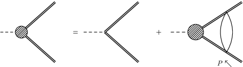
Figure 3: Equation for the effective vertex in the $\lambda\phi^{4}$ theory. The double lines represent the propagators of the hard particles including the $O(\lambda^{2})$ thermal width.

The formula (18) can be applied in order to perform the summation in the vertex equation (24). The term associated with the discontinuities gives (omitting the prefactor $1/2$ and $\rho(Q)$)

$$\int_{-\infty}^{\infty}\frac{d\xi}{2\pi i}\,n_{b}(\xi)\left\{\frac{G(\xi-i\nu_{n},{\mathbf{p}}+{\mathbf{q}})}{\xi-q^{0}-i\omega_{m}-i\nu_{n}}\right.$$

$$\quad\times\left[G^{\rm adv}(\xi,{\mathbf{p}}+{\mathbf{q}})\Lambda_{ij}(\xi-i0^{+},\xi-i\nu_{n})-G^{\rm ret}(\xi,{\mathbf{p}}+{\mathbf{q}})\Lambda_{ij}(\xi+i0^{+},\xi-i\nu_{n})\right]+$$

$$\qquad\qquad\frac{G(\xi+i\nu_{n},{\mathbf{p}}+{\mathbf{q}})}{\xi-q^{0}-i\omega_{m}}$$

$$\quad\times\left.\left[G^{\rm adv}(\xi,{\mathbf{p}}+{\mathbf{q}})\Lambda_{ij}(\xi+i\nu_{n},\xi-i0^{+})-G^{\rm ret}(\xi,{\mathbf{p}}+{\mathbf{q}})\Lambda_{ij}(\xi+i\nu_{n},\xi+i0^{+})\right]\right\},$$ (29)

and the pole term associated with the spectral representation of the rung gives

$$n_{b}(q^{0})G(q^{0}+i\omega_{m}+i\nu_{n},{\mathbf{p}}+{\mathbf{q}})\Lambda_{ij}(q^{0}+i\omega_{m}+i\nu_{n},q^{0}+i\omega_{m})G(q^{0}+i\omega_{m},{\mathbf{p}}+{\mathbf{q}}),$$ (30)

where we have omitted the dependence on ${\mathbf{p}}+{\mathbf{q}}$ in the vertex. After this summation, the analytic continuation $i\omega_{m}+i\nu_{n}\rightarrow p^{0}+\omega+i0^{+},\,i\omega_{m}\rightarrow p^{0}-i0^{+}$ can be explicitly performed

$$\Lambda_{ij}(\xi-i0^{+},\xi-i\nu_{n}) \rightarrow \Lambda_{ij}(\xi-i0^{+},\xi-\omega-i0^{+}),$$

$$\Lambda_{ij}(\xi+i0^{+},\xi-i\nu_{n}) \rightarrow \Lambda_{ij}(\xi+i0^{+},\xi-\omega-i0^{+}),$$

$$\Lambda_{ij}(\xi+i\nu_{n},\xi-i0^{+}) \rightarrow \Lambda_{ij}(\xi+\omega+i0^{+},\xi-i0^{+}),$$

$$\Lambda_{ij}(\xi+i\nu_{n},\xi+i0^{+}) \rightarrow \Lambda_{ij}(\omega+\xi+i0^{+},\xi+i0^{+}),$$

$$G(\xi-i\nu_{n},{\mathbf{p}}+{\mathbf{q}}) \rightarrow G^{\rm adv}(\xi-\omega,{\mathbf{p}}+{\mathbf{q}}),$$

$$G(\xi+i\nu_{n},{\mathbf{p}}+{\mathbf{q}}) \rightarrow G^{\rm ret}(\xi+\omega,{\mathbf{p}}+{\mathbf{q}}).$$

If we neglect the products $G^{\rm adv}G^{\rm adv}$ and $G^{\rm ret}G^{\rm ret}$ as argued before, the discontinuity contribution becomes

$$\int_{-\infty}^{\infty}\frac{d\xi}{2\pi i} G^{\rm ret}(\xi+\omega,{\mathbf{p}}+{\mathbf{q}})\Lambda_{ij}(\xi+\omega+i0^{+},\xi-i0^{+})G^{\rm adv}(\xi,{\mathbf{p}}+{\mathbf{q}})$$ (31)

$$\times\left[\frac{n_{b}(\xi)}{\xi-p^{0}-q^{0}+i0^{+}}-\frac{n_{b}(\xi+\omega)}{\xi-p^{0}-q^{0}-i0^{+}}\right],$$

and the required limit $\omega\rightarrow 0$, after the $\xi$ integration, reduces to

$$-n_{b}(p^{0}+q^{0})G^{\rm ret}(p^{0}+q^{0},{\mathbf{p}}+{\mathbf{q}})\Lambda_{ij}(p^{0}+q^{0}+i0^{+},p^{0}+q^{0}-i0^{+})G^{\rm adv}(p^{0}+q^{0},{\mathbf{p}}+{\mathbf{q}}).$$ (32)

Adding the pole contribution, one finds the integral equation satisfied by the effective vertex

$${\mathcal{D}}_{ij}(P) = \Lambda_{ij}^{(0)}({\mathbf{p}})+\frac{1}{2}\int\frac{d^{4}Q}{(2\pi)^{4}}\,G^{\rm ret}(P+Q){\mathcal{D}}_{ij}(P+Q)G^{\rm adv}(P+Q)$$ (33)

$$\times\rho(Q)\left[n_{b}(q^{0})-n_{b}(p^{0}+q^{0})\right],$$

where we have defined ${\mathcal{D}}_{ij}(p^{0},{\mathbf{p}})\equiv\Lambda_{ij}(p^{0}+i0^{+},p^{0}-i0^{+};{\mathbf{p}})$.

To present a more explicit form of the transport equation, it remains to analyze the product $G^{\rm ret}(P+Q)G^{\rm adv}(P+Q)$. If the momentum $P$ (or $P+Q$) is nearly on-shell, the contribution associated with the sum of the crossed products reduces to a product of two Lorentzians peaked at different values or $p^{0}$. In the limit $\lambda\rightarrow 0$, this fact enables us to neglecting the piece $G_{+}^{\rm ret}G_{-}^{\rm adv}+G_{-}^{\rm ret}G_{+}^{\rm adv}$, so we may write

$$G^{\rm ret}(P+Q)G^{\rm adv}(P+Q)=\sum_{\pm}\frac{1}{4|{\mathbf{p}}+{\mathbf{q}}|^{2}}\frac{1}{(p^{0}+q^{0}\mp|{\mathbf{p}}+{\mathbf{q}}|)^{2}+\Gamma_{{\mathbf{p}}+{\mathbf{q}}}^{2}}$$ (34)

which, for $\lambda\rightarrow 0$, behaves as

$$G^{\rm ret}(P+Q)G^{\rm adv}(P+Q) = \frac{\pi}{4|{\mathbf{p}}+{\mathbf{q}}|^{2}\,\Gamma_{{\mathbf{p}}+{\mathbf{q}}}}\left(\delta(p^{0}+q^{0}-\left|{\mathbf{p}}+{\mathbf{q}}\right|)+\delta(p^{0}+q^{0}+\left|{\mathbf{p}}+{\mathbf{q}}\right|)\right)$$ (35)

$$= \frac{1}{4|{\mathbf{p}}+{\mathbf{q}}|\Gamma_{{\mathbf{p}}+{\mathbf{q}}}}\,2\pi\,\delta\left((p^{0}+q^{0})^{2}-|{\mathbf{p}}+{\mathbf{q}}|^{2}\right)\,.$$

Since the imaginary part of the retarded self-energy is odd in the frequency, the thermal width can be replaced by $-{\rm sgn}(p^{0}+q^{0})\,{\rm Im}\,\Sigma^{\rm ret}(P+Q)/(2\left|{\mathbf{p}}+{\mathbf{q}}\right|)$, and Eq. (35) then becomes

$$G^{\rm ret}(P+Q)G^{\rm adv}(P+Q) = -\frac{1}{2\,{\rm Im}\,\Sigma^{\rm ret}(P+Q)}\,2\pi\,{\rm sgn}(p^{0}+q^{0})\delta\left((p^{0}+q^{0})^{2}-|{\mathbf{p}}+{\mathbf{q}}|^{2}\right)$$ (36)

$$= -\frac{1}{\left(1+n_{b}(p^{0}+q^{0})\right)}\frac{1}{2\,{\rm Im}\,\Sigma^{\rm ret}(P+Q)}G_{0}^{>}(P+Q)\,.$$

With the aid of the identity

$$n_{b}(q^{0})-n_{b}(p^{0}+q^{0})=n_{b}(q^{0})\left(1+n_{b}(p^{0}+q^{0})\right)\left(1-e^{-\beta p^{0}}\right),$$ (37)

one arrives to the final form of the transport equation

$${\mathcal{D}}_{ij}(P)=\Lambda_{ij}^{(0)}({\mathbf{p}})-\left(1-e^{-\beta p^{0}}\right)\int\frac{d^{4}Q}{(2\pi)^{4}}\,L_{\rm Boltz}(-Q)\,G_{0}^{>}(P+Q)\frac{{\mathcal{D}}_{ij}(P+Q)}{2\,{\rm Im}\,\Sigma^{\rm ret}(P+Q)}\,,$$ (38)

in complete agreement with the results of Ref. Jeon , where the equivalence to the linearized Boltzmann equation has been proven. The function ${\mathcal{D}}_{ij}(P)$ is real, even in $p^{0}$, provided that $\rho(Q)$ is odd in $q^{0}$.

The last step in the evaluation of shear viscosity is the computation of the integral (22) for which only the on-shell effective vertex ${\mathcal{D}}_{ij}(p^{0}=p,{\mathbf{p}})$ is required. The insertion of (36) with $P+Q$ replaced by $P$ into (22), and the multiplication by $1/10$ yields the shear viscosity compactly written as

$$\eta=-\frac{\beta}{20}\int\frac{d^{4}P}{(2\pi)^{4}}\,n_{b}(p^{0})\Lambda_{ij}^{(0)}({\mathbf{p}})G^{>}(P)\frac{{\mathcal{D}}_{ij}(P)}{2\,{\rm Im}\,\Sigma^{\rm ret}(P)}\,.$$ (39)

IV Soft contributions to the transport equations in gauge theories

In the derivation of the transport equations that we try, we want emphasize the role played by the screening effects in the regularization of some infrared divergences which arise in the small momentum transfer region. The importance of the dynamical screening in transport phenomena in gauge theories was first recognized in Ref. Baym , where a linearized collision integral free of infrared divergences was stated by using only screened interactions mediated by gauge bosons. Our aim here is to derive transport equations by means of the summation of a restricted set of ladder diagrams, which includes only a specific type of rungs. These rungs will consist of appropriate effective bosonic or fermionic propagators in the hard thermal loop approximation, thus accounting for the screening of distant collisions between all different plasma constituents. Obviously, this approximation does not include the effects due to close collisions and its use requires the imposition of an upper cutoff $q_{c}$ in the integrals over the momentum transfer Yuan . As a check of consistency, we will verify that the coefficients of the UV-logarithmic sensitivities to $q_{c}$ match to the IR-logarithmic divergences previously computed by Arnold, Moore and Yaffe Arnold1 in their treatment of the hard contributions to the collision integrals of the Boltzmann equation.

To elucidate more precisely what type of rungs dominate in the ladder summation which gives the logarithmic accuracy of transport coefficients, it is necessary to estimate the power counting size of the spectral densities which, in our treatment, are associated with the ladder rungs. For instance, consider the spectral density of the rung in the scalar theory of the previous section, Eq. (27). Clearly, it is $O(\lambda^{2})$ from the two vertices, and the contribution $O(\lambda^{-2})$ from the product $G^{\rm ret}G^{\rm adv}$ in Eq. (33) causes the integral term in the vertex equation to have a net $g^{0}$ contribution, as the zero order vertex.

In a gauge theory, there are two possible topologies with the same power counting which potentially contribute to the leading logarithmic order. They are illustrated in Fig. 4. The spectral density of the soft gauge boson exchange ladder, labeled as (a), is $O(1)$ because of the $g^{2}$ suppression from the two vertices, and a $g^{-2}T^{-2}$ contribution from the spectral density of the soft gauge boson. In the $Q$ integration of the vertex equation, similar to Eq. (33), there is a factor $n_{b}(q^{0})=O(g^{-1})$ and a factor $O(g^{-2})$ from the imaginary part of the self-energy in the denominator of the product $\Delta^{\rm ret}\Delta^{\rm adv}$. Finally there is a $g^{3}$ suppression from the soft integration $d^{3}{\mathbf{q}}$ (the contribution of the integration $dq^{0}$ is cancelled by a delta term from $\Delta^{\rm ret}\Delta^{\rm adv}$, see Eqs. (50) and (51) below). Hence, the net contribution of the integral term in the vertex equation is $O(1)$, the same as the zero order vertex, when the spectral density of the rung is also $O(1)$.

Similarly, when the horizontal internal lines are soft gauge boson propagators, the spectral density of the box type ladder rung, labeled as (b) in Fig. 4, is $O(1)$. To perform this estimation, it is helpful to write the general form of the spectral densities in terms of the squares of the $2\leftrightarrow 2$ scattering amplitudes $|\mathcal{M}|^{2}$. Such formulas are similar to Eq. (27)

$$\rho_{\mathrm{a}}(P^{\prime},P) \propto \frac{1}{n_{b}(p^{\prime 0}-p^{0})}\int d^{4}Kd^{4}K^{\prime}\delta^{(4)}(P+K-P^{\prime}-K^{\prime})|\mathcal{M}|^{2}\Delta^{>}(-K^{\prime})\Delta^{>}(K),$$ (40)

$$\rho_{\mathrm{b}}(K^{\prime},P) \propto \frac{1}{n_{b}(k^{\prime 0}-p^{0})}\int d^{4}Kd^{4}P^{\prime}\delta^{(4)}(P+K-P^{\prime}-K^{\prime})|\mathcal{M}|^{2}\Delta^{>}(-P^{\prime})\Delta^{>}(K),$$ (41)

where $P,K,P^{\prime},K^{\prime}$ are the on-shell hard momenta for the particle entering into the scattering processes, and the labels for momenta have been chosen with the aim to use the same $|\mathcal{M}(P,K,P^{\prime},K^{\prime})|^{2}$ within the integrations. For soft momentum transfer $Q=P^{\prime}-P=K-K^{\prime}$, this reduces to

$$|\mathcal{M}(P,K,P^{\prime},K^{\prime})|^{2}\propto g^{4}p^{2}k^{2}|{}^{\ast}\Delta_{\mathrm{L}}(Q)+(\hat{\mathbf{p}}\times\hat{\mathbf{q}})\cdot(\hat{\mathbf{k}}\times\hat{\mathbf{q}}){}^{\ast}\Delta_{\mathrm{T}}(Q)|^{2}\sim O(g^{0})\,,$$ (42)

where ${}^{\ast}\Delta_{\mathrm{L,T}}$ denotes the longitudinal or transverse retarded boson gauge propagator. Note that $P^{\prime}$ and $K$ are loop momenta associated with the integrations in the vertex equation, and $P$ corresponds to the fixed momentum of the effective vertex. In this language, it is easy to recover the power counting size of $\rho_{\mathrm{a}}(P^{\prime},P)$:

$$\rho_{\mathrm{a}}(P^{\prime},P) \propto q^{0}\int_{0}^{\infty}dk\,n_{b,f}^{\prime}(k)\int d\Omega_{\bf k}\delta(q^{0}-\hat{\mathbf{k}}\cdot{\mathbf{q}})|\mathcal{M}|^{2}\propto g^{4}p^{2}T^{2}\frac{q^{0}}{q}\left[|\Delta_{\mathrm{L}}(Q)|^{2}\right.$$ (43)

$$\left.+\frac{1}{2}\left(1-\frac{q_{0}^{2}}{q^{2}}\right)^{2}|\Delta_{\mathrm{T}}(Q)|^{2}\right]\propto g^{2}p^{2}\left[\beta_{\mathrm{L}}(Q)+\left(1-\frac{q_{0}^{2}}{q^{2}}\right)\beta_{\mathrm{T}}(Q)\right]\sim O(g^{0}).$$

For the estimation of $\rho_{\mathrm{b}}(K^{\prime},P)$, the denominator contributes as $g^{0}$ even though $k^{\prime 0}$ and $p^{0}$ are hard energies. The reason for this is that, in general, their difference does not correspond to a soft exchange of energy, as shown in Fig. 4(b). Consequently, $\rho_{\mathrm{b}}(K^{\prime},P)=O(1)$ also.

Figure 4: Two ladder rung topologies of the same power counting. The dashed lines correspond to the cuts giving the spectral densities $\rho_{\mathrm{a}}(P^{\prime},P)$ and $\rho_{\mathrm{b}}(K^{\prime},P)$.

However, in the case of the shear viscosity, the subsequent integration in the vertex equation over the directions of ${\mathbf{k}}^{\prime}$ and the $q^{0}$ integration cancels the contribution of this box type contribution. To understand this cancellation, we note that for small momentum transfer $q\ll p,k$, the energy $\delta$ function which remains after the three-momentum ${\bf p}^{\prime}$ integration in Eq. (41) may be expressed as $\delta(q^{0}-\hat{\mathbf{k}}^{\prime}\cdot{\mathbf{q}})$, and

$$\mathcal{M}(P,K,P^{\prime},K^{\prime})\propto g^{2}pk\left[{}^{\ast}\Delta_{\mathrm{L}}(Q)+{}^{\ast}\Delta_{\mathrm{T}}(Q)\,\left(1-\frac{q_{0}^{2}}{q^{2}}\right)\cos\phi\right]\,,$$ (44)

where $\phi$ is the angle between the planes $({\mathbf{p}},{\mathbf{q}})$ and $({\mathbf{k}}^{\prime},{\mathbf{q}})$. On the other hand, the angular dependence of $\Lambda_{\pi}(K^{\prime})$ within the integration over $K^{\prime}$ in the vertex equation is given by the contraction of $\Lambda_{\pi}(K^{\prime})$ with $\Lambda_{\pi}(P)$, which is proportional to $P_{2}(\cos\theta_{pk^{\prime}})$, with $P_{2}$ the second Legendre polynomial. For small $q$, the required cosine becomes Arnold1

$$\cos\theta_{pk^{\prime}}\simeq\frac{q_{0}^{2}}{q^{2}}+\left(1-\frac{q_{0}^{2}}{q^{2}}\right)\cos\phi\,.$$ (45)

Without screening effects, the boson propagators reduce to ${}^{\ast}\Delta_{L}(Q)=-1/q^{2}$ and ${}^{\ast}\Delta_{T}(Q)=-1/(q_{0}^{2}-q^{2})$. Thus, the angular integration over the azimuthal angle of ${\mathbf{k}}^{\prime}$ followed by the $k^{0}$ (or $q^{0}$) integration turns out to be proportional to

$$\int_{-q}^{q}dq^{0}\int_{0}^{2\pi}d\phi\,P_{2}(\cos\theta_{pk^{\prime}})(1-\cos\phi)^{2}=0\,.$$ (46)

Here, the integration over the spatial range $-q<q^{0}<q$ is enforced by the $\delta(q^{0}-\hat{\mathbf{k}}^{\prime}\cdot{\mathbf{q}})$. This means that the unscreened box rungs do not contribute to the leading logarithmic order and, consequently, box ladder rungs made of two soft gauge boson propagators are irrelevant in order to compute the soft contribution to the shear viscosity.

For the electrical conductivity at zero chemical potentials, the cancellation of these box ladder rungs comes from the charge-conjugation invariance. For each fixed $P$, we have two contributions to the integral term of the vertex equation, corresponding to the insertions of fermions and antifermions through the loop. These contributions are of opposite sign, so their sum vanishes.

Similarly, there are other box ladder rungs in which the horizontal lines are soft fermion propagators, which are comparable to the soft fermion exchange ladders. They do not contribute either to the leading logarithmic order because of the cancellation under angular integration of their unscreened counterparts. Now, the unscreened squared amplitudes are $|\mathcal{M}|^{2}\propto(1-\cos\phi)/q^{2}$ Arnold1 , and the relevant integration is

$$\int_{-q}^{q}dq^{0}\int_{0}^{2\pi}d\phi\,P_{l}(\cos\theta_{pk^{\prime}})(1-\cos\phi)=0\,,$$ (47)

with $l=1,2$ for the electrical conductivity and the shear viscosity, respectively.

Next, let us consider the equations for the effective vertex $\Lambda_{A}$ of a given fermionic species and the effective vertex $\Lambda_{A}^{jm}$ for a given boson gauge. Here, the superindices $(jm)$ denote spatial indices corresponding to the boson propagators in Coulomb gauge to be joined to the vertex, and $A$ collectively denotes the indices corresponding to the insertion of $j_{i}$ or $\pi_{ik}$. We still does not explicitly indicate any spin, color or flavor indices. The equations for the effective vertices are illustrated in Figs. 5 and 6. These equations sum all ladders consisting of rungs made of a HTL gauge boson propagator, and also a HTL fermion propagator. The exchange of a soft gauge boson takes place in scattering between fermions and gauge bosons in non-abelian theories, while the exchange of a soft fermion enters in an annihilation process into a fermionic pair, and the inverse process of creation.

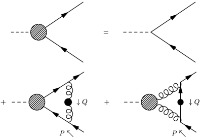
Figure 5: Equation for the soft contribution to the fermionic effective vertex. For the case of the electrical conductivity to leading order in $e$, the soft boson exchanged corresponds to a photon and the last graph is zero.

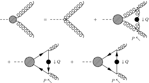
Figure 6: Equation for the soft contribution to the bosonic effective vertex. In the case of the electrical conductivity, all graphs are null.

By following a completely similar treatment to that we have presented for the scalar theory for the summation and analytical continuation to real frequencies, one arrives to the coupled equations for the effective vertices

$$\Lambda_{A}(P)=\Lambda_{A}^{(0)}({\mathbf{p}}) + g^{2}\int\frac{d^{4}Q}{(2\pi)^{4}}\,\gamma^{\mu}S^{\rm ret}(P+Q)\Lambda_{A}(P+Q)S^{\rm adv}(P+Q)\gamma^{\nu}$$ (48)

$$\times{}^{\ast}\rho_{\mu\nu}(Q)\left[n_{b}(q^{0})+n_{f}(p^{0}+q^{0})\right]$$

$$+ g^{2}\int\frac{d^{4}Q}{(2\pi)^{4}}\,G_{ij}^{\rm ret}(P+Q)\Lambda_{A}^{jm}(P+Q)G_{mn}^{\rm adv}(P+Q)\gamma^{i}$$

$$\times{}^{\ast}\rho(\omega,{\mathbf{q}})\gamma^{n}\left[n_{f}(q^{0})+n_{b}(p^{0}+q^{0})\right],$$

and

$$\Lambda_{A}^{jm}(P) = \Lambda_{A}^{(0)\,jm}({\mathbf{p}})+\int\frac{d^{4}Q}{(2\pi)^{4}}\,V^{j\mu k}(P,Q,-P-Q)V^{m\nu n}(-P,-Q,P+Q)$$

$$\times G_{ki}^{\rm ret}(P+Q)\Lambda_{A}^{il}(P+Q)G_{ln}^{\rm adv}(P+Q){}^{\ast}\rho_{\mu\nu}(Q)\left[n_{b}(q^{0})-n_{b}(p^{0}+q^{0})\right]$$

$$+g^{2}\int\frac{d^{4}Q}{(2\pi)^{4}}\,{\rm tr}\left\{\gamma^{j}S^{\rm ret}(P+Q)\Lambda_{A}(P+Q)S^{\rm adv}(P+Q)\gamma^{m}{}^{\ast}\rho(Q)\right.$$

$$-\left.\gamma^{m}S^{\rm ret}(-P-Q)\Lambda_{A}(-P-Q)S^{\rm adv}(-P-Q)\gamma^{j}{}^{\ast}\rho(Q)\right\}\left[n_{f}(q^{0})-n_{f}(p^{0}+q^{0})\right].$$

Here ${}^{\ast}\rho_{\mu\nu}(Q)$ and ${}^{\ast}\rho(Q)$ denote the spectral densities of the soft gauge boson and the fermion and, as usual, $\Lambda_{A}(P)\equiv\Lambda_{A}(p^{0}+i0^{+},p^{0}-i0^{+};{\mathbf{p}})$. Note that we have used the parity properties ${}^{\ast}\rho(Q)={}^{\ast}\rho(-Q)$ and $n_{f}(-q^{0})-n_{f}(-p^{0}-q^{0})=-\left[n_{f}(q^{0})-n_{f}(p^{0}+q^{0})\right]$. These equations are entirely similar to the transport equation for the scalar theory. As there, the occupation numbers $n_{b,f}(p^{0}+q^{0})$ arise from the branch cut contributions, and the identities $n_{b,f}(\xi+n\pi i)=-n_{f,b}(\xi)$ with $n$ odd have been used, if necessary. Further progress requires to examine in detail the explicit structure of the products $S^{\rm ret}\Lambda_{A}S^{\rm adv}$ and $G^{\rm ret}\Lambda_{A}G^{\rm adv}$.

The substitution of the two pieces of the Green’s functions in the product $S^{\rm{ret}}S^{\rm{adv}}$ or $G^{\rm{ret}}G^{\rm{adv}}$ yields four terms, two of them $\Delta_{\pm}^{\rm{ret}}\Delta_{\mp}^{\rm{adv}}$ or $G_{\pm}^{\rm{ret}}G_{\mp}^{\rm{adv}}$ can be directly dropped in the limit $g\rightarrow 0$. Now, by computing the soft contribution to the transport properties, we have only to consider one of the two terms, $++$ or $--$, depending on whether the external momentum corresponds to $p^{0}=p$ or $p^{0}=-p$. This important simplification is due to the fact that, when the external momentum $P$ is on-shell, let’s say $p^{0}=p$, the other sheet of the mass-shell can not be connected by a soft momentum transfer. Clearly, a hard momentum $Q$ is required in order to create two propagating on-shell particles both with hard momentum. In contrast, for the case of the scalar theory, we have retained both terms in Eq. (35) because there, we have not made distinction between soft and hard momentum transfers. Thus, when $P$ is on-shell and $Q\ll P$, we can make the approximations

$$\Delta_{\pm}^{\rm{ret}}(P+Q)\Delta_{\pm}^{\rm{adv}}(P+Q)=\frac{\pi}{\gamma_{{\mathbf{p}}+{\mathbf{q}}}}\,\delta(p^{0}+q^{0}\mp|{\mathbf{p}}+{\mathbf{q}}|)\simeq\frac{\pi}{\gamma_{{\mathbf{p}}+{\mathbf{q}}}}\,\delta(q^{0}\mp\hat{\mathbf{p}}\cdot{\mathbf{q}}),$$ (50)

and

$$G_{\pm}^{\rm{ret}}(P+Q)G_{\pm}^{\rm{adv}}(P+Q)\simeq\frac{\pi}{4p\,|{\mathbf{p}}+{\mathbf{q}}|\,\Gamma_{{\mathbf{p}}+{\mathbf{q}}}}\,\delta(q^{0}\mp\hat{\mathbf{p}}\cdot{\mathbf{q}}).$$ (51)

On the other hand, in the high temperature limit when all masses are negligible, the theory is chirally invariant. As a consequence, the projection operators $h_{\pm}({\hat{\mathbf{p}}})$ can be expressed in terms of simultaneous eigenspinors of chirality and helicity,

$$h_{+}({\hat{\mathbf{p}}}) = u({\hat{\mathbf{p}}},+)\overline{u}({\hat{\mathbf{p}}},+)+u({\hat{\mathbf{p}}},-)\overline{u}({\hat{\mathbf{p}}},-)\,,$$ (52)

$$h_{-}({\hat{\mathbf{p}}}) = v({\hat{\mathbf{p}}},+)\overline{v}({\hat{\mathbf{p}}},+)+v({\hat{\mathbf{p}}},-)\overline{v}({\hat{\mathbf{p}}},-)\,,$$ (53)

where the $u\,(v)$-spinors have the chirality equal (opposite) to the helicity. For example, in the chiral representation, with the momentum along the $3$-axis

$$u({\hat{\mathbf{p}}},+)=\left(\begin{array}[]{c}0\\ 0\\ 1\\ 0\end{array}\right),\quad u({\hat{\mathbf{p}}},-)=\left(\begin{array}[]{c}0\\ 1\\ 0\\ 0\end{array}\right)\quad v({\hat{\mathbf{p}}},+)=\left(\begin{array}[]{c}1\\ 0\\ 0\\ 0\end{array}\right),\quad v({\hat{\mathbf{p}}},-)=\left(\begin{array}[]{c}0\\ 0\\ 0\\ 1\end{array}\right).$$ (54)

In the case of the electrical conductivity, the zero-order effective vertices are

$$\Lambda_{i}^{(0),\,s} = q_{s}e\gamma^{i},$$ (55)

$$\Lambda_{i}^{(0)jm} = 0,$$ (56)

where $q_{s}$ is the charge of the fermionic constituent $s$ in units of $e$. For the shear viscosity, the insertion at zero momentum of a spatially transverse energy-momentum tensor yields the zero-order vertices

$$\Lambda_{ij}^{(0)}({\mathbf{p}}) = \frac{1}{2}\left(\gamma^{i}p^{j}+\gamma^{j}p^{i}-\frac{2}{3}\,{\bm{\gamma}}\cdot{\mathbf{p}}\delta^{ij}\right),$$ (57)

$$\Lambda_{ik}^{(0)jm}({\mathbf{p}}) = 2\left(p^{i}p^{k}-\frac{p^{2}}{3}\delta^{ik}\right)\delta^{jm}.$$ (58)

Both of the fermionic vertices are linear in the $\gamma$-matrices, and this linear dependence is preserved by summing ladder diagrams because each added rung does not introduce any extra dependence. Thus, the fermionic effective vertices, which appear sandwiched between the projection operators $h_{\pm}({\hat{\mathbf{p}}})$ and $h_{\pm}(\widehat{{\mathbf{p}}+{\mathbf{q}}})$ require to consider a $\gamma$-matrix between eigenspinors of all possible chiralities and helicities. Obviously, the combinations between spinors of different chirality, as $\overline{u}(\pm)\gamma^{\mu}u(\mp)$ or $\overline{v}(\pm)\gamma^{\mu}u(\pm)$, are zero. Moreover, the combinations mixing the particle and antiparticle mass shells, as $\overline{v}(\widehat{{\mathbf{p}}+{\mathbf{q}}},\pm)\gamma^{\mu}u({\hat{\mathbf{p}}},\mp)$ or $\overline{u}(\widehat{{\mathbf{p}}+{\mathbf{q}}},\pm)\gamma^{\mu}v({\hat{\mathbf{p}}},\mp)$, do not need to be retained since they can not be connected by a soft momentum transfer. Therefore, we are left with the chirality-independent combinations

$$\overline{u}(\widehat{{\mathbf{p}}+{\mathbf{q}}},\pm)\gamma^{0}u({\hat{\mathbf{p}}},\pm)=1+O(q/p),\qquad\overline{u}(\widehat{{\mathbf{p}}+{\mathbf{q}}},\pm)\gamma^{i}u({\hat{\mathbf{p}}},\pm)=\hat{p}^{i}+O(q/p),$$ (59)

$$\overline{v}(\widehat{{\mathbf{p}}+{\mathbf{q}}},\pm)\gamma^{0}v({\hat{\mathbf{p}}},\pm)=1+O(q/p),\qquad\overline{v}(\widehat{{\mathbf{p}}+{\mathbf{q}}},\pm)\gamma^{i}v({\hat{\mathbf{p}}},\pm)=-\hat{p}^{i}+O(q/p),$$ (60)

corresponding to the lepton (quark) and the anti-lepton (anti-quark), respectively.

IV.1 Soft contribution to the transport equation for the electrical conductivity

Now, we are ready to write more explicitly the transport equations (48) and (IV). For the case of the electrical conductivity, it is suggested to define the non-amputated on-shell vertices for a given charged fermionic species $s$

$${\mathcal{D}}_{i}^{s^{-}}({\mathbf{p}}) \equiv \overline{u}(\hat{{\mathbf{p}}},\pm)\Lambda_{i}^{s}(p^{0}=p,{\mathbf{p}})u({\hat{\mathbf{p}}},\pm),$$ (61)

$${\mathcal{D}}_{i}^{s^{+}}({\mathbf{p}}) \equiv \overline{v}(\hat{{\mathbf{p}}},\pm)\Lambda_{i}^{s}(p^{0}=-p,-{\mathbf{p}})v({\hat{\mathbf{p}}},\pm),$$ (62)

with the corresponding zero-order vertices which follow from Eqs. (59) and (60). Here, the factor $g^{2}$ in the front of the integral in Eq. (48) must be replaced by $q_{s}^{2}e^{2}$. At zero electrical charge, the bosonic effective vertex for electrical conductivity does not enter because its zero-order vanishes, and Furry’s theorem ensures the vanishing of the term within the trace in Eq. (IV). This leaves a single decoupled equation for the fermion vertex.

Next, we fix the external frequency $p^{0}=p$. After multiply both sides of the equation (48) by the $u$-eigenspinors, and expand the integrand using (52)and (50) with $++$, we obtain a term proportional to

$$\delta(q^{0} - \hat{{\mathbf{p}}}\cdot{\mathbf{q}})\overline{u}(\hat{{\mathbf{p}}},\pm)\gamma^{\mu}u(\widehat{{\mathbf{p}}+{\mathbf{q}}},\pm)\,\overline{u}(\widehat{{\mathbf{p}}+{\mathbf{q}}},\pm)\gamma^{\nu}u(\hat{{\mathbf{p}}},\pm)\,{}^{\ast}\rho_{\mu\nu}(Q)=$$ (63)

$$\delta(q^{0}-\hat{{\mathbf{p}}}\cdot{\mathbf{q}})\left[\beta_{\rm L}(Q)+\left(1-\frac{q_{0}^{2}}{q^{2}}\right)\beta_{\rm T}(Q)\right]+O[q/p],$$

where the delta function has enforced a space-like momentum transfer momentum corresponding to Landau damping, and we have used the approximations (59). Finally, the substitution $\Lambda^{i}(\left|{\mathbf{p}}\right|+\hat{{\mathbf{p}}}\cdot{\mathbf{q}},{\mathbf{p}}+{\mathbf{q}})=\Lambda^{i}(\left|{\mathbf{p}}+{\mathbf{q}}\right|,{\mathbf{p}}+{\mathbf{q}})$, valid at soft momentum gives the equation

$${\mathcal{D}}_{i}^{s^{-}}({\mathbf{p}}) = q_{s}e\,\hat{p}^{i}+q_{s}^{2}e^{2}\int\frac{d^{4}Q}{(2\pi)^{4}}\,\pi\delta(q^{0}-\hat{{\mathbf{p}}}\cdot{\mathbf{q}})\left(\frac{T}{q^{0}}-\frac{1}{2}+n_{f}(p)\right)$$ (64)

$$\times\left[\beta_{\rm L}(Q)+\left(1-\frac{q_{0}^{2}}{q^{2}}\right)\beta_{\rm T}(Q)\right]\frac{{\mathcal{D}}_{i}^{s^{-}}({\mathbf{p}}+{\mathbf{q}})}{\gamma_{{\mathbf{p}}+{\mathbf{q}}}^{s}},$$

where we have neglected the $O(q^{0}/p)$ terms in the occupation numbers. Using the parity properties of the zero-order vertex and noting that the spectral density ${}^{\ast}\rho_{\mu\nu}(Q)$ is odd in $q^{0}$, one may easily show from (IV) that ${\mathcal{D}}_{i}^{s^{-}}({\mathbf{p}})=-{\mathcal{D}}_{i}^{s^{+}}({\mathbf{p}})$. This equation is formally similar to the integral equation for the complete leading order of the photon emission rate from the quark-gluon plasma, which has been derived in Ref. Arnold2 .

Following a similar treatment to that used by Arnold, Moore and Yaffe Arnold2 , we may reduce a bit more the transport equation. This proceeds by insertion of the integral for the thermal width of a hard fermion. As we have already said, the thermal width receives the leading order contribution from two-body scattering between fermions by exchange of a soft photon. For a given fermionic species, it is given by the integral Blaizot

$$\gamma_{{\mathbf{p}}}^{(2),s}=q_{s}^{2}e^{2}\int\frac{d^{4}Q}{(2\pi)^{4}}\,\pi\delta(q^{0}-\hat{{\mathbf{p}}}\cdot{\mathbf{q}})\frac{T}{q^{0}}\left[\beta_{\rm L}(Q)+\left(1-\frac{q_{0}^{2}}{q^{2}}\right)\beta_{\rm T}(Q)\right].$$ (65)

Note that the value of this integral remains unaltered when the term $T/q^{0}$ of the integrand is replaced by $T/q^{0}-1/2+n_{f}(p)$. This is due to the fact that the added term $-1/2+n_{f}(p)$ is here multiplied by an odd function of $q^{0}$ and, consequently, is irrelevant. However, this is not true for the corresponding term in (64), since the vectorial dependence of ${\mathcal{D}}_{i}$ on ${\mathbf{p}}+{\mathbf{q}}$ can give odd contributions in ${\mathbf{p}}\cdot{\mathbf{q}}$.

Besides the dominant contribution, the thermal width receives another contribution coming from two-body conversion processes which also give rise to a leading-log term in the transport coefficients. This contribution to the thermal width corresponds to the imaginary part of the diagram of Fig. 7, and it is expressed by the integral

$$\gamma_{{\mathbf{p}}}^{(4),s} = q_{s}^{2}e^{2}\left(\frac{1}{2}+n_{b}(\left|{\mathbf{p}}\right|)\right)\frac{\pi}{2p}\int\frac{d^{4}Q}{(2\pi)^{4}}\,\delta(q^{0}-\hat{{\mathbf{p}}}\cdot{\mathbf{q}})$$ (66)

$$\times\left[\beta_{+}(Q)\left(1-\frac{q^{0}}{q}\right)+\beta_{-}(Q)\left(1+\frac{q^{0}}{q}\right)\right]$$

$$= \frac{q_{s}^{2}e^{2}\omega_{s}^{2}}{8\pi p}\left(1+2n_{b}(\left|{\mathbf{p}}\right|)\right)\left[\ln\left(\frac{q_{c}}{\sqrt{2}\omega_{s}}\right)-1+\ln 2\right],$$

where $q_{c}$ is the upper limit of integration which separates semihard and hard momentum transfers, and $\omega_{s}^{2}=q_{s}^{2}e^{2}T^{2}/8$ is the plasma frequency for the fermionic species $s$.

Figure 7: Subleading contributions to the self-energy of a hard quark (a) and a gluon (b).

By inserting the expression (65) into (64), after defining the quantities

$$\chi_{i}^{s^{-,+}}({\mathbf{p}})\equiv\frac{q_{s}e}{\gamma_{\mathbf{p}}^{s}}\,{\mathcal{D}}_{i}^{s^{-,+}}({\mathbf{p}}),$$ (67)

one obtains a more convenient expression

$$q_{s}^{2}e^{2}\hat{p}^{i} = \gamma_{{\mathbf{p}}}^{(4),s}\,\chi_{i}^{s^{-}}({\mathbf{p}})+q_{s}^{2}e^{2}\int\frac{d^{4}Q}{(2\pi)^{4}}\,\pi\delta(q^{0}-\hat{{\mathbf{p}}}\cdot{\mathbf{q}})\left(\frac{T}{q^{0}}-\frac{1}{2}+n_{f}(p)\right)$$ (68)

$$\times\left[\beta_{\rm L}(Q)+\left(1-\frac{q_{0}^{2}}{{\mathbf{q}}^{2}}\right)\beta_{\rm T}(Q)\right]\left[\chi_{i}^{s^{-}}({\mathbf{p}})-\chi_{i}^{s^{-}}({\mathbf{p}}+{\mathbf{q}})\right],$$

for the soft contribution to the transport equation in the case of electrical conductivity.

An important point to notice here concerns to the absence of some subleading corrections to the hard particle width, whose size is comparable to that included in Eq. (66). Such corrections of $O(g^{3})$ and $O(g^{4}\ln g^{-1})$ arise from the subleading part of the bosonic occupation number $n_{b}(q^{0})$ in the integrand of Eq. (65), and they are associated with

$$n_{b}(q^{0})-\frac{T}{q^{0}}+\frac{1}{2}=2T\sum_{n=1}^{\infty}\frac{q^{0}}{q_{0}^{2}+(2\pi nT)^{2}}.$$ (69)

To understand this absence, consider the transport equation (64) when $\mathcal{D}/\gamma$ has been replaced by $\chi$, as in Eq. (67), and the kernel still contains $n_{b}(q^{0})+n_{f}(p)$. Now, if in the product $\gamma_{\bf p}\chi({\bf p})$ one were to include the subleading terms from Eq. (69), the same terms would have to be included into the occupation number in the kernel of the integral. For small $q$, there is a cancellation between them, and the resulting transport equation would be the same as that in Eq. (68) with $T/q^{0}-1/2+n_{f}(p)$ replaced by $n_{b}(q^{0})+n_{f}(p)$. However, when the momentum $p$ is hard, $n_{f}(p)=O(1)$, and other pole terms different from zero in the occupation number are $O(g)$. Hence, they may be ignored.

IV.2 Soft contribution to the transport equations for shear viscosity

Next, we consider the shear viscosity in a $SU(N_{c})$ gauge theory with $N_{f}$ fermion fields in a given irreducible representation $r$ of dimension $d(r)$. The generator matrices are denoted by $t_{r}^{a}$, and the normalization for this representation is defined by the constant $C(r)$ in ${\rm tr}(t_{r}^{a}t_{r}^{b})=C(r)\delta^{ab}$. The quadratic Casimir operator is denoted by $C_{2}(r)$.

Since the gluon effective vertex $\Lambda_{ik}^{jm,ab}$ is always joined to a pair of transverse projectors of the gauge propagators, it is useful to define the non-amputated on-shell gluon vertex ${\mathcal{D}}_{ik}^{g}$ by

$$P_{T}^{rj}(\hat{\mathbf{p}})\Lambda_{ik}^{jm,ab}(p^{0}=\left|{\mathbf{p}}\right|,{\mathbf{p}})P_{T}^{ms}(\hat{\mathbf{p}})\equiv{\mathcal{D}}_{ik}^{g}({\mathbf{p}})P_{\rm T}^{rs}(\hat{\mathbf{p}})\delta^{ab},$$ (70)

and the zero-order vertex corresponding to Eq. (58), ${\mathcal{D}}_{ik}^{(0)\,g}({\mathbf{p}})=2(p^{i}p^{k}-\delta^{ik}{\mathbf{p}}^{2}/3)$. On the other hand, and as before, we define the the non-amputated on-shell quark vertex ${\mathcal{D}}_{ik}^{q}$ by

$${\mathcal{D}}_{ik}^{q}({\mathbf{p}})\equiv\overline{u}(\hat{\mathbf{p}},\pm)\Lambda_{ik}(p^{0}=p,{\mathbf{p}})u(\hat{\mathbf{p}},\pm),$$ (71)

and the zero-order vertex corresponding to Eq. (57), ${\mathcal{D}}_{ik}^{(0)\,q}({\mathbf{p}})=|{\mathbf{p}}|(\hat{p}^{i}\hat{p}^{k}-\delta^{ik}/3)$. We note that the similar vertex for anti-quarks, ${\mathcal{D}}^{\overline{q}}=\overline{v}\Lambda(-P)v$, turns out to be the same as for quarks, as it is easily checked by examining the corresponding zero-order vertices, and noting that each added rung in the iteration does not break this property.

Now, in order to derive the transport equations for ${\mathcal{D}}_{ik}^{q,\,g}$, it only remains to perform the appropriate contraction of Eqs. (48) and (IV) with a pair of $u$-spinors and a pair of transverse projectors, respectively. Using the approximations

$$\overline{u}(\hat{\mathbf{p}},\pm)\gamma^{m}\left[\beta_{+}(Q)h_{+}({\mathbf{q}})+\beta_{-}(Q)h_{-}({\mathbf{q}})\right]\gamma^{n}u(\hat{\mathbf{p}},\pm)P_{\rm T}^{mn}(\widehat{{\mathbf{p}}+{\mathbf{q}}})=$$

$$\qquad\qquad\beta_{+}(Q)\left(1-\hat{\mathbf{p}}\cdot\hat{\mathbf{q}}\right)+\beta_{-}(Q)\left(1+\hat{\mathbf{p}}\cdot\hat{\mathbf{q}}\right)+O(q/p),$$ (72)

$${\rm tr}\left\{\gamma^{m}h_{+}(\widehat{{\mathbf{p}}+{\mathbf{q}}})\gamma^{n}\left[\beta_{+}(Q)h_{+}({\mathbf{q}})+\beta_{-}(Q)h_{-}({\mathbf{q}})\right]\right\}P_{\rm T}^{mr}(\hat{\mathbf{p}})P_{\rm T}^{ns}(\hat{\mathbf{p}})=$$

$$\qquad\qquad\left[\beta_{+}(Q)\left(1-\hat{\mathbf{p}}\cdot\hat{\mathbf{q}}\right)+\beta_{-}(Q)\left(1+\hat{\mathbf{p}}\cdot\hat{\mathbf{q}}\right)\right]P_{\rm T}^{rs}(\hat{\mathbf{p}})+O(q/p),$$ (73)

and

$$f^{acd}f^{bcd}V^{j\mu k}(P,Q,-P-Q)V^{m\nu n}(-P,-Q,P+Q){}^{\ast}\rho_{\mu\nu}(Q)P_{\rm T}^{kn}(\widehat{{\mathbf{p}}+{\mathbf{q}}})P_{\rm T}^{jr}(\hat{\mathbf{p}})P_{\rm T}^{ms}(\hat{\mathbf{p}})=$$

$$\qquad\qquad 4g^{2}N_{c}\,{\mathbf{p}}^{2}\left[\beta_{\rm L}(Q)+\left(1-\hat{\mathbf{p}}\cdot\hat{\mathbf{q}}^{2}\right)\beta_{\rm T}(Q)\right]P_{\rm T}^{rs}(\hat{\mathbf{p}})\delta^{ab}+O(q/p),$$ (74)

one finds

$${\mathcal{D}}_{ik}^{q}({\mathbf{p}}) = {\mathcal{D}}_{ik}^{(0)\,q}({\mathbf{p}})+g^{2}C_{2}(r)\int\frac{d^{4}Q}{(2\pi)^{4}}\,\pi\delta(q^{0}-\hat{{\mathbf{p}}}\cdot{\mathbf{q}})\,{\mathcal{B}}(Q)\left(\frac{T}{q^{0}}-\frac{1}{2}+n_{f}(p)\right)\frac{{\mathcal{D}}_{ik}^{q}({\mathbf{p}}+{\mathbf{q}})}{\gamma_{{\mathbf{p}}+{\mathbf{q}}}}$$ (75)

$$+g^{2}C_{2}(r)\int\frac{d^{4}Q}{(2\pi)^{4}}\,\pi\delta(q^{0}-\hat{{\mathbf{p}}}\cdot{\mathbf{q}})\,{\mathcal{F}}(Q)\left(\frac{1}{2}+n_{b}(p)\right)\frac{{\mathcal{D}}_{ik}^{g}({\mathbf{p}}+{\mathbf{q}})}{4p\,\left|{\mathbf{p}}+{\mathbf{q}}\right|\Gamma_{{\mathbf{p}}+{\mathbf{q}}}},$$

and a completely similar for the gluon vertex

$${\mathcal{D}}_{ik}^{g}({\mathbf{p}}) = {\mathcal{D}}_{ik}^{(0)\,g}({\mathbf{p}})+g^{2}N_{c}\left|{\mathbf{p}}\right|\int\frac{d^{4}Q}{(2\pi)^{4}}\,\pi\delta(q^{0}-\hat{{\mathbf{p}}}\cdot{\mathbf{q}})\,{\mathcal{B}}(Q)\left(\frac{T}{q^{0}}-\frac{1}{2}-n_{b}(p)\right)\frac{{\mathcal{D}}_{ik}^{g}({\mathbf{p}}+{\mathbf{q}})}{\left|{\mathbf{p}}+{\mathbf{q}}\right|\Gamma_{{\mathbf{p}}+{\mathbf{q}}}}$$ (76)

$$+2g^{2}N_{f}C(r)\int\frac{d^{4}Q}{(2\pi)^{4}}\,\pi\delta(q^{0}-\hat{{\mathbf{p}}}\cdot{\mathbf{q}})\,{\mathcal{F}}(Q)\left(\frac{1}{2}-n_{f}(p)\right)\frac{{\mathcal{D}}_{ik}^{q}({\mathbf{p}}+{\mathbf{q}})}{\gamma_{{\mathbf{p}}+{\mathbf{q}}}},$$

where

$${\mathcal{B}}(Q) \equiv \beta_{\rm L}(Q)+\left(1-\frac{q_{0}^{2}}{{\mathbf{q}}^{2}}\right)\beta_{\rm T}(Q)\,,$$ (77)

$${\mathcal{F}}(Q) \equiv \beta_{+}(Q)\left(1-\frac{q^{0}}{q}\right)+\beta_{-}(Q)\left(1+\frac{q^{0}}{q}\right)\,.$$ (78)

Note that we have approximated the occupation numbers by their expansions up to $O(q^{0})$ corrections. The prefactor $2$ in front of the piece $g^{2}N_{f}C(r)$ in the last term of (76) is due to the two possible orientations for the momentum in the quark loop. The remainder of the previous equations is almost obvious, after performing the approximations (50) and (51).

Finally, as for the case of electrical conductivity, in order to make more clear the closed resemblance of these equations with Boltzmann-type equations, we may define the quantities which will turn to correspond to the deviations from the equilibrium distribution functions of quarks and gluons,

$$\chi_{ik}^{q}({\mathbf{p}}) \equiv \frac{{\mathcal{D}}_{ik}^{q}({\mathbf{p}})}{\gamma_{\mathbf{p}}}\,,$$ (79)

$$\chi_{ik}^{g}({\mathbf{p}}) \equiv \frac{{\mathcal{D}}_{ik}^{g}({\mathbf{p}})}{2|{\mathbf{p}}|\,\Gamma_{\mathbf{p}}}\,.$$ (80)

Then, the substitution of thermal widths by their integral representations yields the final form of the soft contribution to the coupled transport equations for these quantities. They become

$$|{\mathbf{p}}|(\hat{p}^{i}\hat{p}^{k}-\frac{1}{3}\delta^{ik})=$$

$$\qquad g^{2}C_{2}(r)\int\frac{d^{4}Q}{(2\pi)^{4}}\,\pi\delta(q^{0}-\hat{{\mathbf{p}}}\cdot{\mathbf{q}})\,{\mathcal{B}}(Q)\left(\frac{T}{q^{0}}-\frac{1}{2}+n_{f}(p)\right)\left[\chi_{ik}^{q}({\mathbf{p}})-\chi_{ik}^{q}({\mathbf{p}}+{\mathbf{q}})\right]$$

$$\quad+\frac{g^{2}C_{2}(r)}{2|{\mathbf{p}}|}\left(\frac{1}{2}+n_{b}(p)\right)\int\frac{d^{4}Q}{(2\pi)^{4}}\,\pi\delta(q^{0}-\hat{{\mathbf{p}}}\cdot{\mathbf{q}}){\mathcal{F}}(Q)\left[\chi_{ik}^{q}({\mathbf{p}})-\chi_{ik}^{g}({\mathbf{p}}+{\mathbf{q}})\right]\,,$$ (81)

and

$$|{\mathbf{p}}|(\hat{p}^{i}\hat{p}^{k}-\frac{1}{3}\delta^{ik})=$$

$$\qquad g^{2}N_{c}\int\frac{d^{4}Q}{(2\pi)^{4}}\,\pi\delta(q^{0}-\hat{{\mathbf{p}}}\cdot{\mathbf{q}})\,{\mathcal{B}}(Q)\left(\frac{T}{q^{0}}-\frac{1}{2}-n_{b}(p)\right)\left[\chi_{ik}^{g}({\mathbf{p}})-\chi_{ik}^{g}({\mathbf{p}}+{\mathbf{q}})\right]$$

$$\quad+\frac{g^{2}N_{f}C_{2}(r)}{|{\mathbf{p}}|}\left(\frac{1}{2}-n_{f}(p)\right)\int\frac{d^{4}Q}{(2\pi)^{4}}\pi\delta(q^{0}-\hat{{\mathbf{p}}}\cdot{\mathbf{q}})\,{\mathcal{F}}(Q)\left[\chi_{ik}^{g}({\mathbf{p}})-\chi_{ik}^{q}({\mathbf{p}}+{\mathbf{q}})\right]\,.$$ (82)

V Extracting the leading-log transport coefficients from the soft contribution

Rotational invariance fixes the form of the $\chi$-functions. In the case of electrical conductivity, they have the form

$$\chi_{i}^{s^{-}}({\mathbf{p}})=\hat{p}^{i}\chi^{s^{-}}(p),$$ (83)

and for shear viscosity,

$$\chi_{ik}^{q,\,g}({\mathbf{p}})=\left(\hat{p}^{i}\hat{p}^{k}-\frac{1}{3}\delta^{ik}\right)\chi^{q,\,g}(p).$$ (84)

When $|{\mathbf{q}}|\ll|{\mathbf{p}}|$, we may to approximate the integral collision terms in the transport equations by a derivative expansion of the $\chi$-functions, in a similar way to the procedure which leads to the derivation of Fokker-Planck equations in the context of classical plasmas Gasiorowicz ; Rosenbluth . With the aim to extract the leading-log terms for the transport coefficients, we only require the insertion into the transport equations of the second-order approximations for the quantities $\hat{p}^{i}\left[\chi_{i}^{s^{-}}({\mathbf{p}})-\chi_{i}^{s^{-}}({\mathbf{p}}+{\mathbf{q}})\right]$ and $\hat{p}^{i}\hat{p}^{k}\left[\chi_{ik}^{q,\,g}({\mathbf{p}})-\chi_{ik}^{q,\,g}({\mathbf{p}}+{\mathbf{q}})\right]$. At the same accuracy, terms of the type $\left[\chi_{ik}^{q,\,g}({\mathbf{p}})-\chi_{ik}^{g,\,q}({\mathbf{p}}+{\mathbf{q}})\right]$ are replaced by $\left[\chi_{ik}^{q,\,g}({\mathbf{p}})-\chi_{ik}^{g,\,q}({\mathbf{p}})\right]$. These substitutions produce a combination of derivatives of the $\chi$-functions, whose coefficients are integral expressions involving the Landau damping piece of soft spectral densities. Here, the leading-log terms will arise from to the logarithmic dependence on the upper limit $q_{c}$. Although the computation of the complete leading order in $g$ of these integrals can need numerical quadrature, the leading-log order is easily obtained analytically by means of the formulas based on sum rules given in the appendix B.

After the angular integration of the Eqs. (IV.2) and (IV.2), and the subsequent $q^{0}$ integration with the aid of Eqs. (114) and (118), the logarithmic terms finally combine to give the following expressions in the case of shear viscosity

$$p = -\frac{g^{2}C_{2}(r)m_{D}^{2}T}{16\pi}\ln g^{-1}\left\{\chi^{q}(p)^{\prime\prime}+\left[\frac{2}{p}-\frac{1}{T}(1-2n_{f}(p))\right]\chi^{q}(p)^{\prime}-\frac{6}{p^{2}}\chi^{q}(p)\right\}$$ (85)

$$+\frac{g^{2}C_{2}(r)\omega_{0}^{2}}{8\pi p}\ln g^{-1}\left(1+2n_{b}(p)\right)\left[\chi^{q}(p)-\chi^{g}(p)\right],$$

$$p = -\frac{g^{2}N_{c}m_{D}^{2}T}{16\pi}\ln g^{-1}\left\{\chi^{g}(p)^{\prime\prime}+\left[\frac{2}{p}-\frac{1}{T}(1+2n_{b}(p))\right]\chi^{g}(p)^{\prime}-\frac{6}{p^{2}}\chi^{g}(p)\right\}$$ (86)

$$+\frac{g^{2}N_{f}C(r)\omega_{0}^{2}}{4\pi p}\ln g^{-1}\left(1-2n_{f}(p)\right)\left[-\chi^{q}(p)+\chi^{g}(p)\right],$$

where $\ln g^{-1}$ is the term coming from either $\ln\left(\frac{q_{c}}{m_{D}}\right)$ or $\ln\left(\frac{q_{c}}{\omega_{0}}\right)$ with logarithmic accuracy, and

$$m_{D}^{2} = \frac{g^{2}T^{2}}{3}\left[N_{c}+N_{f}C(r)\right],$$ (87)

$$\omega_{0}^{2} = \frac{g^{2}T^{2}}{8}\,C_{2}(r).$$ (88)

Quite remarkably, the terms $(1\pm 2n_{b,\,f}(p))/T$ multiplying the first derivatives and generated by the zero-order in $q^{0}$ of $n_{b}(q^{0})\mp n_{b\,,f}(p+q^{0})$, allow us to write a single functional of $\chi^{q}(p)$ and $\chi^{g}(p)$ whose variation leads to above equations for shear viscosity in the leading-log approximation. This functional $\int_{0}^{\infty}dp\,{\mathcal{L}}(\chi,\chi^{\prime})$ turns out to be exactly the same as that previously found by Arnold, Moore and Yaffe Arnold1 in their derivation of the leading-log terms of the linearized collision integral of the Boltzmann equation. After multiplication of both sides of Eqs. (85) and (86) by $2d(r)N_{f}p^{2}n_{f}(p)(1-n_{f}(p))$ and $d(G)p^{2}n_{b}(p)(1+n_{b}(p))$ respectively, one finds

$${\mathcal{L}}(\chi,\chi^{\prime}) = -2d(r)N_{f}p^{3}n_{f}(p)(1-n_{f}(p))\chi^{q}(p)-d(G)p^{3}n_{b}(p)(1+n_{b}(p))\chi^{g}(p)$$ (89)

$$+\frac{g^{2}N_{f}\omega_{0}^{2}d(r)C_{2}(r)}{8\pi}\ln g^{-1}\,p\,n_{f}(p)(1+n_{b}(p))\left[\chi^{q}(p)-\chi^{g}(p)\right]^{2}$$

$$+\frac{g^{2}N_{f}m_{D}^{2}Td(r)C_{2}(r)}{16\pi}\ln g^{-1}\,n_{f}(p)(1-n_{f}(p))\left[p^{2}\chi^{q}(p)^{\prime 2}+6\chi^{q}(p)^{2}\right]$$

$$+\frac{g^{2}N_{c}m_{D}^{2}Td(G)}{32\pi}\ln g^{-1}\,n_{b}(p)(1+n_{b}(p))\left[p^{2}\chi^{g}(p)^{\prime 2}+6\chi^{g}(p)^{2}\right],$$

where we have used $d(r)C_{2}(r)=d(G)C(r)$ with $d(G)=N_{c}^{2}-1$.

Using the expressions (22) and (11), and noting that $({\hat{p}}^{i}{\hat{p}}^{k}-\delta^{ik}/3)({\hat{p}}^{i}{\hat{p}}^{k}-\delta^{ik}/3)=2/3$, we see that the contribution to the shear viscosity of each Dirac fermion is

$$\frac{\beta}{15\pi^{2}}\int_{0}^{\infty}dp\,p^{3}n_{f}(p)(1-n_{f}(p))\chi^{q}(p),$$ (90)

while each gauge boson contributes as

$$\frac{\beta}{30\pi^{2}}\int_{0}^{\infty}dp\,p^{3}n_{b}(p)(1+n_{b}(p))\chi^{g}(p).$$ (91)

Hence, the shear viscosity is exactly the value of the functional $-\beta/(15\pi^{2})\int_{0}^{\infty}dp\,{\mathcal{L}}$ for the values of $\chi$ solving the motion equations.

For the electrical conductivity, the above procedure applied to Eq. (68) yields the expression

$$1 = -\frac{m_{D}^{2}T}{16\pi}\ln e^{-1}\left\{\chi^{s^{-}}(p)^{\prime\prime}+\left[\frac{2}{p}-\frac{1}{T}(1-2n_{f}(p))\right]\chi^{s^{-}}(p)^{\prime}-\frac{2}{p^{2}}\chi^{s^{-}}(p)\right\}$$ (92)

$$+\frac{\omega_{s}^{2}}{8\pi p}\ln e^{-1}\left(1+2n_{b}(p)\right)\chi^{s^{-}}(p),$$

where the Debye mass for the photon and the plasma frequency for the charged fermionic species $s$ are given by

$$m_{D}^{2} = \frac{e^{2}T^{2}}{3}\left(N_{\rm leptons}+d(r)\sum_{\rm quarks}q_{s}^{2}\right)$$ (93)

$$\omega_{s}^{2} = \frac{q_{s}^{2}e^{2}T^{2}}{8}.$$ (94)

This equation may be retrieved by varying the functional $\int_{0}^{\infty}dp\,{\mathcal{L}}^{s}(\chi,\chi^{\prime})$, where ${\mathcal{L}}^{s}$ may be chosen as

$${\mathcal{L}}^{s} = -p^{2}n_{f}(p)(1-n_{f}(p))\chi^{s^{-}}(p)+\frac{\omega_{s}^{2}}{16\pi}\ln e^{-1}p\,n_{f}(p)(1+n_{b}(p))\chi^{s^{-}}(p)^{2}$$ (95)

$$+\frac{m_{D}^{2}T}{32\pi}\ln e^{-1}n_{f}(p)(1-n_{f}(p))\left[p^{2}\chi^{s^{-}}(p)^{\prime 2}+2\chi^{s^{-}}(p)^{2}\right].$$

Now, the contribution of each charged Dirac fermion to the electrical conductivity is

$$\frac{\beta}{3\pi^{2}}\int_{0}^{\infty}dp\,p^{2}n_{f}(p)(1-n_{f}(p))\chi^{s^{-}}(p),$$ (96)

which implies that this transport coefficient is given by $-2\beta/(3\pi^{2})\sum_{s}\int_{0}^{\infty}dp\,{\mathcal{L}}^{s}$ at the stationary values of $\chi^{s^{-}}$.

This completes the derivation of the leading-log terms for the transport coefficients. The agreement with the results of Ref. Arnold1 is complete when the conversions $\chi^{q,g}\rightarrow-2\beta\chi_{\rm AMY}^{q,g}$, $\chi^{s^{-}}\rightarrow-2\beta\chi_{\rm AMY}^{e^{+}}$ are performed, and the sum over charged species is restricted to leptons.

VI Conclusion and prospects

In this paper we have shown how to derive transport equations in some relativistic many body theories from the summation of uncrossed ladder diagrams within the imaginary time formalism. The procedure is similar to the one used in a quite remote past by Holstein Holstein and, for the case of the scalar field theory, yields the correct results previously derived by Jeon Jeon . In this treatment, one first identifies the analytic continuation to real frequencies for the effective vertex, and then writes the integral equation which it satisfies. The two relevant quantities in the vertex equation turn out to be the imaginary part of the self-energy and the spectral weight of the ladder rung.

For the case of gauge theories, we have derived a couple of transport equations (68), (IV.2) and (IV.2) by resummation of the ladder series, whose graphs are made of the rungs associated with resummed propagators in the HTL approximation. The kernels of the integral equations derived in this way are the same as the integrands of thermal widths for hard particles to leading and next to leading order. By extracting the logarithmic terms, the transport equations turn out to be differential equations similar to Fokker-Planck equations which appear as approximations to the collision integrals in Coulomb plasmas. The $O(g^{4}\ln 1/g)$ thermal widths in these equations are seen as damping terms, similar to those which arise when the Boltzmann equation is treated in the relaxation time approximation. These differential equations are the same as those recently found by Arnold, Moore and Yaffe Arnold1 by analyzing the infrared divergences of the linearized collision integrals without screened interactions. Thus, this fact constitutes a non trivial check of the formalism we have used and also of the HTL approximation, because of the correct matching of the UV-divergences in our approach with the infrared divergences in the approach of Ref. Arnold1 .

With respect to the computation of the complete leading order of the transport coefficients, we believe that, in analogy with the scalar theory, the introduction of all rungs made of the one-loop four-point functions may be of interest. Obviously, most of these rungs will lead to non divergent results, and only a few of them would yield the infrared divergences of the hard contribution matching with the logarithmic divergences we have found here. To carry out these computations within the framework we have presented, the classification of the four-point functions and the corresponding spectral densities would have to be studied.

Appendix A The spectral density of the rung in $\lambda\phi^{4}$ theory

In this appendix, the spectral density in Eq. (27) is calculated. The product of two free Matsubara propagators is conveniently written as the double spectral representation

$$G_{0}(i\nu_{q} + i\nu_{k},{\mathbf{q}}+{\mathbf{k}})G_{0}(i\nu_{k},{\mathbf{k}})=\int\int\frac{d\omega_{1}\,d\omega_{2}}{(2\pi)^{2}}\frac{1}{i\nu_{q}-\omega_{2}}$$ (97)

$$\times\left[\frac{\rho_{0}(\omega_{1}+\omega_{2},{\mathbf{q}}+{\mathbf{k}})\rho_{0}(\omega_{1},{\mathbf{k}})}{i\nu_{k}-\omega_{1}}-\frac{\rho_{0}(\omega_{1},{\mathbf{q}}+{\mathbf{k}})\rho_{0}(\omega_{1}-\omega_{2},{\mathbf{k}})}{i\nu_{q}+i\nu_{k}-\omega_{1}}\right],$$

where $\rho_{0}(p^{0},{\mathbf{p}})=2\pi\,{\rm sgn}(p^{0})\,\delta((p^{0})^{2}-p^{2})$. By performing the sum over $\nu_{k}$, and taking the imaginary part of the analytic continuation $i\nu_{q}\rightarrow q^{0}+i0^{+}$, one obtains

$$\rho(Q) = \int\frac{d^{3}{\mathbf{k}}\,d\omega_{1}}{(2\pi)^{4}}\,n_{b}(\omega_{1})$$ (98)

$$\times\left[\rho_{0}(\omega_{1}+q^{0},{\mathbf{q}}+{\mathbf{k}})\rho_{0}(\omega_{1},{\mathbf{k}})-\rho_{0}(\omega_{1},{\mathbf{q}}+{\mathbf{k}})\rho_{0}(\omega_{1}-q^{0},{\mathbf{k}})\right].$$

The second piece of this integral may be rearranged by a shift of the $\omega_{1}$ integration, $\omega_{1}\rightarrow\omega_{1}+q^{0}$. Thus, after the use of the parity property $\rho_{0}(\omega_{1}+q^{0},{\mathbf{q}}+{\mathbf{k}})=-\rho_{0}(-\omega_{1}-q^{0},-{\mathbf{q}}-{\mathbf{k}}))$, and the substitution

$$\rho_{0}(-k^{0}-q^{0},-{\mathbf{q}}-{\mathbf{k}})=\frac{1}{1+n_{b}(-k^{0}-q^{0})}\,G_{0}^{>}(-K-Q),$$ (99)

Eq. (98) yields the desired result

$$\rho(Q)=(e^{\beta q^{0}}-1)\int\frac{d^{4}K}{(2\pi)^{4}}G_{0}^{>}(-K-Q)G_{0}^{>}(K).$$ (100)

Appendix B Sum rules

The required integrals over the Landau damping range of the frequency follow from the sum rules Lebellac derived from the analytic properties of the effective propagators. With the notation of Ref. Blaizot , these sum rules are

$$\int_{-q}^{q}\frac{dq^{0}}{2\pi}\frac{1}{q^{0}}\,{}^{\ast}\beta_{\rm L}(Q) = \frac{m_{D}^{2}}{q^{2}\left(q^{2}+m_{D}^{2}\right)}-\frac{z_{\rm L}(q)}{\omega_{\rm L}(q)^{2}},$$ (101)

$$\int_{-q}^{q}\frac{dq^{0}}{2\pi}\,q^{0}\,{}^{\ast}\beta_{\rm L}(Q) = \frac{m_{D}^{2}}{3q^{2}}-z_{\rm L}(q),$$ (102)

$$\int_{-q}^{q}\frac{dq^{0}}{2\pi}(q^{0})^{3}\,{}^{\ast}\beta_{\rm L}(Q) = \frac{m_{D}^{2}}{5}+\frac{m_{D}^{4}}{9q^{2}}-z_{\rm L}(q)\omega_{\rm L}(q)^{2},$$ (103)

$$\int_{-q}^{q}\frac{dq^{0}}{2\pi}\frac{1}{q^{0}}\,{}^{\ast}\beta_{\rm T}(Q) = \frac{1}{q^{2}}-\frac{z_{\rm T}(q)}{\omega_{\rm T}(q)^{2}},$$ (104)

$$\int_{-q}^{q}\frac{dq^{0}}{2\pi}\,q^{0}\,{}^{\ast}\beta_{\rm T}(Q) = 1-z_{\rm T}(q),$$ (105)

$$\int_{-q}^{q}\frac{dq^{0}}{2\pi}(q^{0})^{3}\,{}^{\ast}\beta_{\rm T}(Q) = q^{2}+\frac{m_{D}^{2}}{3}-z_{\rm T}(q)\omega_{\rm T}(q)^{2},$$ (106)

where $z_{\rm L,T}(q)$ are the residues at the quasi-particle poles. With the aim to extract the logarithmic dependence of the transport equations on $q_{c}$, we use the the approximations valid at large $q$, $q\gg m_{D}$,

$$z_{\rm L}(q) = \frac{8q^{2}}{m_{D}^{2}}\,\exp\left(-2-\frac{2q^{2}}{m_{D}^{2}}\right),$$ (107)

$$z_{\rm T}(q) = 1+\frac{3m_{D}^{2}}{4q^{2}}\left[1+\frac{1}{3}\ln\left(\frac{m_{D}^{2}}{8q^{2}}\right)\right],$$ (108)

$$\omega_{\rm L}(q)^{2} = q^{2}\left[1+4\exp\left(-2-\frac{2q^{2}}{m_{D}^{2}}\right)\right],$$ (109)

$$\omega_{\rm T}(q)^{2} = q^{2}+\frac{m_{D}^{2}}{2}+\frac{m_{D}^{4}}{4q^{2}}\left[1+\frac{1}{2}\ln\left(\frac{m_{D}^{2}}{8q^{2}}\right)\right],$$ (110)

and we find the quadratic terms in $m_{D}^{2}$ which give rise to the logarithmic terms $\ln(q_{c}/m_{D})$ after the $q$ integration,

$$\int_{-q}^{q}\frac{dq^{0}}{2\pi}(q^{0})^{2n-1}{}^{\ast}\beta_{\rm L}(Q) \approx \frac{m_{D}^{2}}{q^{4-2n}}\times\left\{\begin{array}[]{ll}1&\quad n=0\\ 1/3&\quad n=1\\ 1/5&\quad n=2\end{array}\right.,$$ (114)

$$\int_{-q}^{q}\frac{dq^{0}}{2\pi}(q^{0})^{2n-1}{}^{\ast}\beta_{\rm T}(Q) \approx \frac{m_{D}^{2}}{q^{4-2n}}\times\left\{\begin{array}[]{ll}-1/4&\quad n=0\\ -3/4&\quad n=1\\ -11/12&\quad n=2\end{array}\right..$$ (118)

The explicit form of the functions $\beta_{\rm L}$ and $\beta_{\rm T}$ is

$$\beta_{\rm L}(q_{0},{\mathbf{q}}) = \frac{4\pi m_{D}^{2}\,q_{0}\,q\,\theta(q^{2}-q_{0}^{2})}{4q^{2}\left\{q^{2}+m_{D}^{2}[1-Q(q_{0}/q)]\right\}^{2}+\pi^{2}m_{D}^{4}q_{0}^{2}},$$ (119)

$$\beta_{\rm T}(q_{0},{\mathbf{q}}) = \frac{8\pi m_{D}^{2}\,q_{0}\,q^{3}(q^{2}-q_{0}^{2})\,\theta(q^{2}-q_{0}^{2})}{4q^{2}\left\{(q^{2}-q_{0}^{2})\left[2q^{2}+m_{D}^{2}Q(q_{0}/q)\right]+m_{D}^{2}q_{0}^{2}\right\}^{2}+\pi^{2}m_{D}^{4}q_{0}^{2}(q^{2}-q_{0}^{2})^{2}},$$ (120)

where the function $Q(x)$ is given by

$$Q(x)=\frac{x}{2}\ln\frac{1+x}{1-x}\,.$$ (121)

Appendix C Thermal widths

To leading order in $g$ ($e$), the thermal width of a hard particle is obtained by the insertion of one HTL gluon (photon) propagator into the skeleton graph for the one-loop self-energy. For a hard quark (or a charged fermionic species $s$), the resulting expression is Blaizot

$$\gamma_{p}^{(2)}=g^{2}C_{2}(r)\,T\int\frac{d^{4}Q}{(2\pi)^{4}}\,\pi\delta(q^{0}-\hat{{\mathbf{p}}}\cdot{\mathbf{q}})\frac{1}{q^{0}}\left[\beta_{\rm L}(Q)+\left(1-\frac{q_{0}^{2}}{q^{2}}\right)\beta_{\rm T}(Q)\right],$$ (122)

with $g^{2}C_{2}(r)$ replaced by $q_{s}^{2}e^{2}$ in the case of a charged fermion. For a hard gluon, the same expression is valid if $C_{2}(r)\rightarrow N_{c}$.

Next, we present the expressions for the thermal widths for hard particles to order $g^{4}\ln g^{-1}$. The fermion self-energy is showed in Fig. 7, and is written as

$$\Sigma(i\omega_{n},{\mathbf{p}})=-g^{2}C_{2}(r)\,T\sum_{\nu_{n}}\int\frac{d^{3}{\mathbf{q}}}{(2\pi)^{3}}\,\gamma^{\mu}\,{}^{\ast}S(i\nu_{n}+i\omega_{n},{\mathbf{p}}+{\mathbf{q}})\gamma^{\nu}G_{\mu\nu}(i\nu_{n},{\mathbf{q}}).$$ (123)

Making use of the spectral representation of the soft fermion in the HTL approximation,

$${}^{\ast}S(i\omega_{n},{\mathbf{q}})=\int_{-\infty}^{\infty}\frac{dq^{0}}{2\pi}\frac{{}^{\ast}\Delta_{+}(Q)h_{+}(\hat{{\mathbf{q}}})+{}^{\ast}\Delta_{-}(Q)h_{-}(\hat{{\mathbf{q}}})}{q^{0}-i\omega_{n}},$$ (124)

with ${}^{\ast}\Delta_{\pm}$ verifying the parity properties

$${}^{\ast}\Delta_{\pm}(q^{0},{\mathbf{q}})={}^{\ast}\Delta_{\mp}(-q^{0},{\mathbf{q}}),$$ (125)

we may perform the Matsubara sum. After, one may extract the imaginary part of the continuation $i\omega_{n}\rightarrow p^{0}+i0^{+}$. When $p^{0}=p$, the dominant contribution comes from the piece of the integrand which multiplies to $\delta(p^{0}-q^{0}-\left|{\mathbf{p}}-{\mathbf{k}}\right|)$. The replacement of this delta by $\delta(q^{0}-\hat{\mathbf{p}}\cdot{\mathbf{q}})$, valid for $q\ll p$, selects the Landau damping piece of ${}^{\ast}\Delta_{\pm}$, and the expansion of the remaining terms to lowest order in $q/p$ yields

$$\gamma_{p}^{(4)} = -\frac{1}{4p}\,{\rm{tr}}\left({\hbox to0.0pt{\hbox to5.03125pt{\hfil/\hfil}\hss}p}\,{\rm Im}\,\Sigma^{\rm ret}(p^{0}=p,{\mathbf{p}})\right)=-\overline{u}(\hat{\mathbf{p}},\pm)\Sigma^{\rm ret}(p^{0}=p,{\mathbf{p}})u(\hat{\mathbf{p}},\pm)$$ (126)

$$= \frac{g^{2}C_{2}(r)}{2p}\left(\frac{1}{2}+n_{b}(p)\right)\int\frac{d^{4}Q}{(2\pi)^{4}}\,\pi\delta(q^{0}-\hat{{\mathbf{p}}}\cdot{\mathbf{q}}){\mathcal{F}}(Q),$$

where

$${\mathcal{F}}(Q)\equiv\beta_{+}(Q)\left(1-\frac{q^{0}}{q}\right)+\beta_{-}(Q)\left(1+\frac{q^{0}}{q}\right).$$ (127)

The spectral functions $\beta_{\pm}(Q)$ are given by

$$\beta_{\pm}(q_{0},{\mathbf{q}})=\frac{\pi\omega_{0}^{2}q_{0}^{2}(q\mp q_{0})\theta(q^{2}-q_{0}^{2})}{\left[\pm q_{0}q(q\mp q_{0})+\omega_{0}^{2}\left\{\pm q_{0}[1-Q(q_{0}/q)]+q\,Q(q_{0}/q)\right\}\right]^{2}+\frac{\pi^{2}\omega_{0}^{4}q_{0}^{2}(q\mp q_{0})^{2}}{4q^{2}}},$$ (128)

where the frequency plasma for the fermion is $\omega_{0}^{2}=g^{2}C_{2}(r)T^{2}/8$ or $q_{s}^{2}e^{2}T^{2}/8$. The integral (126) has been treated in refs.  Arnold3 ; Kapusta ; Aurenche and, for $q_{c}\gg\omega_{s}$, gives

$$\int\frac{d^{4}Q}{(2\pi)^{4}}\,\pi\delta(q^{0}-\hat{{\mathbf{p}}}\cdot{\mathbf{q}}){\mathcal{F}}(Q)=\frac{\omega_{0}^{2}}{2\pi}\left[\ln\left(\frac{q_{c}}{\sqrt{2}\omega_{s}}\right)-1+\ln 2\right].$$ (129)

The $O(g^{4}\ln g^{-1})$ thermal width for a hard gauge boson is associated with the imaginary part of the self-energy of the diagram in Fig. 7. It reads

$$\Pi_{\mu\nu}(i\omega_{n},{\mathbf{p}})=2N_{f}\,g^{2}C(r)\,T\sum_{\nu_{n}}\int\frac{d^{3}{\mathbf{q}}}{(2\pi)^{3}}\,{\rm tr}\left\{\gamma_{\mu}\,S(i\nu_{n}+i\omega_{n},{\mathbf{p}}+{\mathbf{q}})\gamma_{\nu}{}^{\ast}S(i\nu_{n},{\mathbf{q}})\right\},$$ (130)

where the prefactor $2$ comes from the two possible ways to arrange a soft fermion propagator in the graph. A similar treatment to the fermionic case leads to the result

$$\Gamma_{p}^{(4)} = -\frac{1}{2p}\,{\rm Im}\,\Pi_{\rm T}^{\rm ret}(p^{0}=p,{\mathbf{p}})$$ (131)

$$= \frac{g^{2}N_{f}C(r)}{p}\left(\frac{1}{2}-n_{f}(p)\right)\int\frac{d^{4}Q}{(2\pi)^{4}}\,\pi\delta(q^{0}-\hat{{\mathbf{p}}}\cdot{\mathbf{q}}){\mathcal{F}}(Q),$$

where $\Pi_{\rm T}(P)=\Pi_{ij}(\delta^{ij}-\hat{p}^{i}\hat{p}^{j})/2$. For the case of a hard photon, the correct result is obtained with the substitutions $g^{2}N_{f}C(r)\rightarrow e^{2}\sum_{\rm charged\,species}q_{s}^{2}$ and $\omega_{0}\rightarrow\omega_{s}$.

References

- (1) G. Baym, H. Monien, C. J. Pethick and D. G. Ravenhall, Phys. Rev. Lett. 64, 1867 (1990).
- (2) H. Heiselberg, G. Baym, C. J. Pethick and J. Popp, Nucl. Phys. A 544, 569C (1992); H. Heiselberg, Phys. Rev. Lett. 72, 3013 (1994) [arXiv:hep-ph/9401317]; H. Heiselberg, Phys. Rev. D 49, 4739 (1994) [arXiv:hep-ph/9401309].
- (3) G. Baym and H. Heiselberg, Phys. Rev. D 56, 5254 (1997) [arXiv:astro-ph/9704214].
- (4) P. Arnold, G. D. Moore and L. G. Yaffe, JHEP 0011, 001 (2000) [arXiv:hep-ph/0010177].
- (5) G. D. Moore, JHEP 0105, 039 (2001) [arXiv:hep-ph/0104121].
- (6) G. D. Mahan, Many-Particle Physics, third edition, (Kluwer Academic/Plenum Publishers, New York, 2000), ISBN 0 306 46338 5.
- (7) S. Jeon, Phys. Rev. D 52, 3591 (1995) [arXiv:hep-ph/9409250].
- (8) M. E. Carrington, H. Defu and R. Kobes, Phys. Rev. D 62, 025010 (2000) [arXiv:hep-ph/9910344]; M. E. Carrington, H. Defu and R. Kobes, Phys. Lett. B 523, 221 (2001) [arXiv:hep-ph/0106292].
- (9) E. Wang and U. W. Heinz, Phys. Lett. B 471, 208 (1999) [arXiv:hep-ph/9910367]; E. Wang and U. W. Heinz, arXiv:hep-th/0201116.
- (10) J. M. Martínez Resco and M. A. Valle Basagoiti, Phys. Rev. D 63, 056008 (2001) [arXiv:hep-ph/0009331].
- (11) P. Arnold, G. D. Moore and L. G. Yaffe, JHEP 0111, 057 (2001) [arXiv:hep-ph/0109064].
- (12) P. Arnold, G. D. Moore and L. G. Yaffe, JHEP 0112, 009 (2001) [arXiv:hep-ph/0111107].
- (13) T. Holstein, Ann. Phys. (N.Y.) 29, 410 (1964).
- (14) E. Braaten and R. D. Pisarski, Nucl. Phys. B337, (1990) 569; J. Frenkel and J. Taylor, Nucl. Phys. B334, 199 (1990); J. Taylor and S. Wong, Nucl. Phys. B346, 115 (1990).
- (15) E. Braaten and T. C. Yuan, Phys. Rev. Lett. 66, 2183 (1991); E. Braaten and M. H. Thoma, Phys. Rev. D 44, 1298 (1991).
- (16) J. P. Blaizot and E. Iancu, Phys. Rept. 359, 355 (2002) [arXiv:hep-ph/0101103].
- (17) S. Gasiorowicz, M. Neumann and R. J. Ridell, Phys. Rev. 101, 922 (1956).
- (18) M. R. Rosenbluth, W. M. MacDonald and D. L. Judd, Phys. Rev. 107, 1 (1957).
- (19) J. Kapusta, P. Lichard and D. Seibert, Phys. Rev. D 44 (1991) 2774 [Erratum-ibid. D 47 (1991) 4171].
- (20) P. Aurenche, F. Gelis, R. Kobes and E. Petitgirard, Z. Phys. C 75, 315 (1997) [arXiv:hep-ph/9609256].
- (21) M. Le Bellac, Thermal Field Theory, (Cambridge University Press, Cambridge, England, 1996), ISBN 0 521 46040 9.