$K$-matrix analysis of the $(IJ^{PC}=00^{++})$-wave in the mass region below $1900$ MeV

Abstract

We present the results of the current analysis of the partial wave $IJ^{PC}=00^{++}$ based on the available data for meson spectra ($\pi\pi,K\bar{K},\eta\eta,\eta\eta^{\prime},\pi\pi\pi\pi$). In the framework of the $K$-matrix approach, the analytical amplitude has been restored in the mass region $280$ MeV$<\sqrt{s}<1900$ MeV. The following scalar-isoscalar states are seen: comparatively narrow resonances $f_{0}(980)$, $f_{0}(1300)$, $f_{0}(1500)$, $f_{0}(1750)$ and the broad state $f_{0}(1200-1600)$. The positions of the amplitude poles (masses and total widths of the resonances) are determined as well as pole residues (partial widths to meson channels $\pi\pi,K\bar{K},\eta\eta,\eta\eta^{\prime},\pi\pi\pi\pi$). The fitted amplitude gives us the positions of the $K$-matrix poles (bare states) and the values of bare-state couplings to meson channels thus allowing the quark-antiquark nonet classification of bare states. On the basis of the obtained partial widths to the channels $\pi\pi,K\bar{K},\eta\eta,\eta\eta^{\prime}$, we estimate the quark/gluonium content of $f_{0}(980)$, $f_{0}(1300)$, $f_{0}(1500)$, $f_{0}(1750)$, $f_{0}(1200-1600)$. For $f_{0}(980)$, $f_{0}(1300)$, $f_{0}(1500)$ and $f_{0}(1750)$, their partial widths testify the $q\bar{q}$ origin of these mesons though being unable to provide precise evaluation of the possible admixture of the gluonium component in these resonances. The ratios of the decay coupling constants for the $f_{0}(1200-1600)$ support the idea about gluonium nature of this broad state.

1 Introduction

The classification of meson states in the scalar-isoscalar sector is a key problem for understanding the strong QCD being a subject of intensive discussions in recent years, see, for example, [1, 2, 3, 4, 5, 6, 7] and references therein.

In this paper we present the results of the $K$-matrix analysis of the $00^{++}$ wave in the invariant mass range 280–1900 MeV. This analysis is a continuation of earlier work [5, 8, 9, 10, 11]. In the latter paper [11], the $00^{++}$ wave had been reconstructed on the basis of the following data set:
(1) GAMS data on the $S$-wave two-meson production in the reactions $\pi p\to\pi^{0}\pi^{0}n$, $\eta\eta n$ and $\eta\eta^{\prime}n$ at small nucleon momenta transferred, $|t|<0.2$ (GeV/$c$)² [12, 13];
(2) GAMS data on the $\pi\pi$ $S$-wave production in the reaction $\pi p\to\pi^{0}\pi^{0}n$ at large momenta transferred, $0.30<|t|<1.0$ (GeV/$c$)² [12];
(3) BNL data on $\pi p^{-}\to K\bar{K}n$ [14];
(4) CERN-Münich data on $\pi^{+}\pi^{-}\to\pi^{+}\pi^{-}$ [15];
(5) Crystal Barrel data on $p\bar{p}$(at rest, from liquid $H_{2}$)$\to\pi^{0}\pi^{0}\pi^{0}$, $\pi^{0}\pi^{0}\eta$, $\pi^{0}\eta\eta$ [16].

Now the experimental basis has been much broadened, and additional samples of data are included into present analysis of the $00^{++}$ wave, as follows:
(6) Crystal Barrel data on proton-antiproton annihilation in gas: $p\bar{p}$(at rest, from gaseous $H_{2}$)$\to\pi^{0}\pi^{0}\pi^{0}$, $\pi^{0}\pi^{0}\eta$ [17, 18],
(7) Crystal Barrel data on proton-antiproton annihilation in liquid: $p\bar{p}$(at rest, from liquid $H_{2}$)$\to\pi^{+}\pi^{-}\pi^{0}$, $K^{+}K^{-}\pi^{0}$, $K_{S}K_{S}\pi^{0}$, $K^{+}K_{S}\pi^{-}$ [17, 18];
(8) Crystal Barrel data on neutron-antiproton annihilation in the liquid deuterium: $n\bar{p}$(at rest, from liquid $D_{2}$)$\to\pi^{0}\pi^{0}\pi^{-}$, $\pi^{-}\pi^{-}\pi^{+}$, $K_{S}K^{-}\pi^{0}$, $K_{S}K_{S}\pi^{-}$ [17, 18];
(9) E852 Collaboration data on the $\pi\pi$ $S$-wave production in the reaction $\pi^{-}p\to\pi^{0}\pi^{0}n$ at the nucleon momentum transfers squared $0<|t|<1.5\;({\rm GeV/c})^{2}$ [19].

The production of resonances in the $00^{++}$ wave is accompanied by a considerable background. This circumstance forces us to carry out a simultaneous analysis of as much as possible number of spectra, for only in such an analysis one can single out resonance parameters reliably.

As compared to the paper [11], the reactions of the $p\bar{p}$ annihilation in gas have been included into the present analysis. One should keep in mind that, while in the liquid hydrogene the $p\bar{p}$ annihilation is going dominantly from the $S$-state, in the gas there is a large admixture of the $P$-wave, thus providing us an opportunity to analyse three-meson Dalitz plots in more detail.

New Crystal Barrel data allow us to study the two-kaon channel more reliably as compared to what had been done before. This is undoubtedly important for the conclusion about the quark-gluonium content of the $f_{0}$-mesons under investigation.

The data of the E852 Collaboration on the reaction $\pi^{-}p\to\pi^{0}\pi^{0}n$ at $p_{lab}=18$ GeV/c [19] together with GAMS data on the rection $\pi^{-}p\to\pi^{0}\pi^{0}n$ at $p_{lab}=38$ GeV/c [12] give us a good opportunity for the study the resonances $f_{0}(980)$ and $f_{0}(1300)$, for at large momenta transferred to the nucleon, $|t|\sim 0.5\sim 1.5$ (GeV/c)², the production of resonances goes with a small background thus allowing us to fix convincingly their masses and widths. This is especially important for $f_{0}(1300)$: in the compilation [20] this resonance is referred as $f_{0}(1370)$, with the mass in the interval $1200-1500$ MeV, though experimental data favour the mass near 1300 MeV.

In Section 2 we present a set of formulae for the analysed $K$-matrix amplitudes as follows:
(i) the $K$-matrix amplitudes of the mass-on-shell transitions into channels $\pi\pi,K\bar{K},\eta\eta,\eta\eta^{\prime},\pi\pi\pi\pi$;
(ii) the $K$-matrix amplitudes for the transitions $\pi\pi^{(R)}(t)\to\pi\pi$ and $\pi a^{(R)}_{1}(t)\to\pi\pi$, where $\pi^{(R)}(t)$ and $a^{(R)}_{1}(t)$ are reggeized pion and $a_{1}$-meson in the high energy reaction $\pi^{-}p\to(\pi\pi)_{S}\;n$;
(iii) the $K$-matrix three-meson production amplitudes in the $p\bar{p}$ and $n\bar{p}$ annihilations.

The $K$-matrix amplitude determines both the amplitude poles (masses and widths of resonances) and the $K$-matrix poles (masses of bare states). The $K$-matrix poles differ from the amplitude poles in two points:
(i) The states corresponding to the $K$-matrix poles do not contain any component associated with real mesons which are inherent in resonances. The absence of a cloud of real mesons allows us to refer conventionally to these states as bare ones [5, 9, 11].
(ii) Due to the transitions bare state(1) $\to$ real mesons $\to$ bare state(2) the observed resonances are the mixtures of bare states. So, for the quark systematics, bare states are the primary objects rather than resonances.

In Section 3, we present the main results of the present analysis. As in previous papers, we have had three solutions which are denoted, following [11], Solutions I, II-1 and II-2. In all Solutions, the characteristics of the resonances $f_{0}(980)$, $f_{0}(1300)$, $f_{0}(1500)$ and broad state $f_{0}(1200-1600)$ coincide with each other and coincide, with a reasonable accuracy, with what had been obtained in [11]. From this point of view, the performed analysis provided us with unambigously determined properties of physical states, with an exception for the resonance $f_{0}(1750)$, for which the channel $f_{0}(1750)\to\pi\pi\pi\pi$ is not well defined, that resulted in different full widths given by Solutions I and II. Solutions I, II-1 and II-2 differ by the characteristics of bare states and background terms in the $K$-matrix, just as it was the case in [11], though it must be particularly emphasized that the present analysis reveals a noticeable tendency for the parametrs from different Solutions to become closer to each other. In the present analysis the distinction in characteristics of bare states is not dramatic with an exception, again, for $f_{0}(1750)$, for which the coupling constant of the $K$-matrix pole to the channel $\pi\pi\pi\pi$ given by Solutions I and II have opposite sign.

The relations between coupling constants of the $q\bar{q}$ bare state, $f_{0}^{bare}$, to channels $\pi\pi$, $K\bar{K}$, $\eta\eta$, $\eta\eta^{\prime}$ provide us with an information on the relative weight of the components $n\bar{n}=(u\bar{u}+d\bar{d})/\sqrt{2}$ and $s\bar{s}$. For the gluoniun, the relations between coupling constants are nearly the same as for the flavour $q\bar{q}$ singlet, thus leading to the ambiguity in the definition of the glueball: Solutions I, II-1 and II-2 provided us with different possibilities for the glueball among bare states.

In Solution I, there are two bare states, every of them pretending to be the glueball: $f^{bare}_{0}(1220\pm 30)$ and $f^{bare}_{0}(1635\pm 25)$. In Solution II-1 only one state, $f^{bare}_{0}(1225\pm 25)$, satisfies the constraint inherent in the glueball. In Solution II-2, again there are two states whose coupling constants are appropriate to the glueball: $f^{bare}_{0}(1230\pm 30)$ and $f^{bare}_{0}(1560\pm 25)$ . The uncertainty in the classification of bare states, which is based on the value of a coupling to channels $f_{0}^{bare}\to\pi\pi,K\bar{K},\eta\eta,\eta\eta^{\prime}$, makes us to apply the other methods to single out the states which are extra ones for the $q\bar{q}$-systematics, namely, exotic states. The method based on the consideration of trajectories in the $(n,M^{2})$-plane ($n$ is radial quantum number of the $q\bar{q}$ state and $M$ its mass) is discussed in Section 5.

On the basis of the extracted partial widths for the channels $\pi\pi$, $K\bar{K}$, $\eta\eta$, $\eta\eta^{\prime}$, the following properties of resonances $f_{0}(980)$, $f_{0}(1300)$, $f_{0}(1500)$, $f_{0}(1750)$ and broad state $f_{0}(1200-1600)$ are to claim:

1. $f_{0}(980)$: This resonance is dominantly the $q\bar{q}$ state, $q\bar{q}=n\bar{n}\sin\varphi+s\bar{s}\cos\varphi$, with a large $s\bar{s}$ component. Under the assumption that the admixture of the glueball component is not greater than 15%, $W_{gluonium}\mathrel{\mathchoice{\lower 3.6pt\vbox{\halign{$\mathsurround=0pt\displaystyle\hfil#\hfil$\cr<\crcr\sim\crcr}}}{\lower 3.6pt\vbox{\halign{$\mathsurround=0pt\textstyle\hfil#\hfil$\cr<\crcr\sim\crcr}}}{\lower 3.6pt\vbox{\halign{$\mathsurround=0pt\scriptstyle\hfil#\hfil$\cr<\crcr\sim\crcr}}}{\lower 3.6pt\vbox{\halign{$\mathsurround=0pt\scriptscriptstyle\hfil#\hfil$\cr<\crcr\sim\crcr}}}}15\%$, the hadronic decays give us the following constraints: $-95^{\circ}\leq\varphi\mathrel{\mathchoice{\lower 3.6pt\vbox{\halign{$\mathsurround=0pt\displaystyle\hfil#\hfil$\cr<\crcr\sim\crcr}}}{\lower 3.6pt\vbox{\halign{$\mathsurround=0pt\textstyle\hfil#\hfil$\cr<\crcr\sim\crcr}}}{\lower 3.6pt\vbox{\halign{$\mathsurround=0pt\scriptstyle\hfil#\hfil$\cr<\crcr\sim\crcr}}}{\lower 3.6pt\vbox{\halign{$\mathsurround=0pt\scriptscriptstyle\hfil#\hfil$\cr<\crcr\sim\crcr}}}}-40^{\circ}$, that is in agreement with data on radiative decays $f_{0}(980)\to\gamma\gamma$ and $\phi(1020)\to\gamma f_{0}(980)$ [21, 22]. Rather large uncertainties in the determination of mixing angle are due to the sensitivity of coupling constants to plausible small admixtures of the gluonium. If the gluonium component is absent, hadronic decays provide $\varphi=-67^{\circ}\pm 10^{\circ}$.

As concern the characteristics of the $f_{0}(980)$, we cannot observe any special property which would single it out from a $q\bar{q}$ series: it belongs to linear $q\bar{q}$ trajectory on the $(n,M^{2})$ and $(J,M^{2})$ planes and its decay couplings to hadronic channels are of the same order as for the other $f_{0}$ resonances, see Table 5 in Section 4. Besides, this resonance is produced, without any suppression, in hard processes as well as in heavy-quark decays, e.g. in the reactions $\pi^{-}p\to(\pi\pi)_{S}\;n$ at large $|t|$ [12, 19] and $D^{+}_{s}\to\pi^{+}\pi^{+}\pi^{-}$ [23].

2. $f_{0}(1300)$: This resonance is the descendant of the bare $q\bar{q}$ state which is close to the flavour singlet. The resonance $f_{0}(1300)$ is formed due to a strong mixing with the primary gluonium and neighbouring $q\bar{q}$ states. The $q\bar{q}$ content, $q\bar{q}=n\bar{n}\cos\varphi+s\bar{s}\sin\varphi$, in the $f_{0}(1300)$ strongly depends on the admixture of the gluonium component. At $W_{gluonium}\mathrel{\mathchoice{\lower 3.6pt\vbox{\halign{$\mathsurround=0pt\displaystyle\hfil#\hfil$\cr<\crcr\sim\crcr}}}{\lower 3.6pt\vbox{\halign{$\mathsurround=0pt\textstyle\hfil#\hfil$\cr<\crcr\sim\crcr}}}{\lower 3.6pt\vbox{\halign{$\mathsurround=0pt\scriptstyle\hfil#\hfil$\cr<\crcr\sim\crcr}}}{\lower 3.6pt\vbox{\halign{$\mathsurround=0pt\scriptscriptstyle\hfil#\hfil$\cr<\crcr\sim\crcr}}}}30\%$ the mixing angle changes, depending on $W_{gluonium}$, in the interval $-45^{\circ}\mathrel{\mathchoice{\lower 3.6pt\vbox{\halign{$\mathsurround=0pt\displaystyle\hfil#\hfil$\cr<\crcr\sim\crcr}}}{\lower 3.6pt\vbox{\halign{$\mathsurround=0pt\textstyle\hfil#\hfil$\cr<\crcr\sim\crcr}}}{\lower 3.6pt\vbox{\halign{$\mathsurround=0pt\scriptstyle\hfil#\hfil$\cr<\crcr\sim\crcr}}}{\lower 3.6pt\vbox{\halign{$\mathsurround=0pt\scriptscriptstyle\hfil#\hfil$\cr<\crcr\sim\crcr}}}}\varphi[f_{0}(1300)]\mathrel{\mathchoice{\lower 3.6pt\vbox{\halign{$\mathsurround=0pt\displaystyle\hfil#\hfil$\cr<\crcr\sim\crcr}}}{\lower 3.6pt\vbox{\halign{$\mathsurround=0pt\textstyle\hfil#\hfil$\cr<\crcr\sim\crcr}}}{\lower 3.6pt\vbox{\halign{$\mathsurround=0pt\scriptstyle\hfil#\hfil$\cr<\crcr\sim\crcr}}}{\lower 3.6pt\vbox{\halign{$\mathsurround=0pt\scriptscriptstyle\hfil#\hfil$\cr<\crcr\sim\crcr}}}}25^{\circ}$; at $W_{gluonium}=0$ the hadronic decays provide $\varphi[f_{0}(1300)]=-7^{\circ}\pm 10^{\circ}$.

3. $f_{0}(1500)$: The resonance is the descendant of the bare state with a large $n\bar{n}$ component. Being similar to $f_{0}(1300)$, the resonance $f_{0}(1500)$ is formed by mixing with the gluonium as well as with neighbouring $q\bar{q}$ states. The $q\bar{q}$ content, $q\bar{q}=n\bar{n}\cos\varphi+s\bar{s}\sin\varphi$, depends on the admixture of the gluonium: at $W_{gluonium}\mathrel{\mathchoice{\lower 3.6pt\vbox{\halign{$\mathsurround=0pt\displaystyle\hfil#\hfil$\cr<\crcr\sim\crcr}}}{\lower 3.6pt\vbox{\halign{$\mathsurround=0pt\textstyle\hfil#\hfil$\cr<\crcr\sim\crcr}}}{\lower 3.6pt\vbox{\halign{$\mathsurround=0pt\scriptstyle\hfil#\hfil$\cr<\crcr\sim\crcr}}}{\lower 3.6pt\vbox{\halign{$\mathsurround=0pt\scriptscriptstyle\hfil#\hfil$\cr<\crcr\sim\crcr}}}}30\%$ the mixing angle changes, depending on $W_{gluonium}$, in the interval $-20^{\circ}\mathrel{\mathchoice{\lower 3.6pt\vbox{\halign{$\mathsurround=0pt\displaystyle\hfil#\hfil$\cr<\crcr\sim\crcr}}}{\lower 3.6pt\vbox{\halign{$\mathsurround=0pt\textstyle\hfil#\hfil$\cr<\crcr\sim\crcr}}}{\lower 3.6pt\vbox{\halign{$\mathsurround=0pt\scriptstyle\hfil#\hfil$\cr<\crcr\sim\crcr}}}{\lower 3.6pt\vbox{\halign{$\mathsurround=0pt\scriptscriptstyle\hfil#\hfil$\cr<\crcr\sim\crcr}}}}\varphi[f_{0}(1500)]\mathrel{\mathchoice{\lower 3.6pt\vbox{\halign{$\mathsurround=0pt\displaystyle\hfil#\hfil$\cr<\crcr\sim\crcr}}}{\lower 3.6pt\vbox{\halign{$\mathsurround=0pt\textstyle\hfil#\hfil$\cr<\crcr\sim\crcr}}}{\lower 3.6pt\vbox{\halign{$\mathsurround=0pt\scriptstyle\hfil#\hfil$\cr<\crcr\sim\crcr}}}{\lower 3.6pt\vbox{\halign{$\mathsurround=0pt\scriptscriptstyle\hfil#\hfil$\cr<\crcr\sim\crcr}}}}25^{\circ}$; at $W_{gluonium}=0$ one has $\varphi[f_{0}(1500)]=10^{\circ}\pm 10^{\circ}$.

4. $f_{0}(1750)$: This resonance is the descendant of the bare state of the radial excitation nonet $2^{3}P_{1}q\bar{q}$, which flavour wave function has large $s\bar{s}$ component. In Solutions I and II, the resonance $f_{0}(1750)$ has different values of the $s\bar{s}$ component. In Solution I, the $s\bar{s}$ component dominates: in the absence of gluonium component, $\varphi[f_{0}(1750)]=-72^{\circ}\pm 5^{\circ}$, and if the gluonium admixture is $W_{gluonium}\mathrel{\mathchoice{\lower 3.6pt\vbox{\halign{$\mathsurround=0pt\displaystyle\hfil#\hfil$\cr<\crcr\sim\crcr}}}{\lower 3.6pt\vbox{\halign{$\mathsurround=0pt\textstyle\hfil#\hfil$\cr<\crcr\sim\crcr}}}{\lower 3.6pt\vbox{\halign{$\mathsurround=0pt\scriptstyle\hfil#\hfil$\cr<\crcr\sim\crcr}}}{\lower 3.6pt\vbox{\halign{$\mathsurround=0pt\scriptscriptstyle\hfil#\hfil$\cr<\crcr\sim\crcr}}}}30\%$, then $-110^{\circ}\mathrel{\mathchoice{\lower 3.6pt\vbox{\halign{$\mathsurround=0pt\displaystyle\hfil#\hfil$\cr<\crcr\sim\crcr}}}{\lower 3.6pt\vbox{\halign{$\mathsurround=0pt\textstyle\hfil#\hfil$\cr<\crcr\sim\crcr}}}{\lower 3.6pt\vbox{\halign{$\mathsurround=0pt\scriptstyle\hfil#\hfil$\cr<\crcr\sim\crcr}}}{\lower 3.6pt\vbox{\halign{$\mathsurround=0pt\scriptscriptstyle\hfil#\hfil$\cr<\crcr\sim\crcr}}}}\varphi[f_{0}(1750)]\mathrel{\mathchoice{\lower 3.6pt\vbox{\halign{$\mathsurround=0pt\displaystyle\hfil#\hfil$\cr<\crcr\sim\crcr}}}{\lower 3.6pt\vbox{\halign{$\mathsurround=0pt\textstyle\hfil#\hfil$\cr<\crcr\sim\crcr}}}{\lower 3.6pt\vbox{\halign{$\mathsurround=0pt\scriptstyle\hfil#\hfil$\cr<\crcr\sim\crcr}}}{\lower 3.6pt\vbox{\halign{$\mathsurround=0pt\scriptscriptstyle\hfil#\hfil$\cr<\crcr\sim\crcr}}}}-35^{\circ}$. In Solution II, in the absence of gluonium component, $\varphi[f_{0}(1750)]=-27^{\circ}\pm 10^{\circ}$, and with gluonium admixture $W_{gluonium}\mathrel{\mathchoice{\lower 3.6pt\vbox{\halign{$\mathsurround=0pt\displaystyle\hfil#\hfil$\cr<\crcr\sim\crcr}}}{\lower 3.6pt\vbox{\halign{$\mathsurround=0pt\textstyle\hfil#\hfil$\cr<\crcr\sim\crcr}}}{\lower 3.6pt\vbox{\halign{$\mathsurround=0pt\scriptstyle\hfil#\hfil$\cr<\crcr\sim\crcr}}}{\lower 3.6pt\vbox{\halign{$\mathsurround=0pt\scriptscriptstyle\hfil#\hfil$\cr<\crcr\sim\crcr}}}}30\%$, $-50^{\circ}\mathrel{\mathchoice{\lower 3.6pt\vbox{\halign{$\mathsurround=0pt\displaystyle\hfil#\hfil$\cr<\crcr\sim\crcr}}}{\lower 3.6pt\vbox{\halign{$\mathsurround=0pt\textstyle\hfil#\hfil$\cr<\crcr\sim\crcr}}}{\lower 3.6pt\vbox{\halign{$\mathsurround=0pt\scriptstyle\hfil#\hfil$\cr<\crcr\sim\crcr}}}{\lower 3.6pt\vbox{\halign{$\mathsurround=0pt\scriptscriptstyle\hfil#\hfil$\cr<\crcr\sim\crcr}}}}\varphi[f_{0}(1750)]\mathrel{\mathchoice{\lower 3.6pt\vbox{\halign{$\mathsurround=0pt\displaystyle\hfil#\hfil$\cr<\crcr\sim\crcr}}}{\lower 3.6pt\vbox{\halign{$\mathsurround=0pt\textstyle\hfil#\hfil$\cr<\crcr\sim\crcr}}}{\lower 3.6pt\vbox{\halign{$\mathsurround=0pt\scriptstyle\hfil#\hfil$\cr<\crcr\sim\crcr}}}{\lower 3.6pt\vbox{\halign{$\mathsurround=0pt\scriptscriptstyle\hfil#\hfil$\cr<\crcr\sim\crcr}}}}10^{\circ}$.

5. $f_{0}(1200-1600)$: The broad state is the descendant of a primary glueball. The analysis of hadronic decays of this resonance confirms its glueball nature, for the $q\bar{q}$ component is allowed to be in a state produced by the glueball: $(q\bar{q})_{glueball}=(\sqrt{2}n\bar{n}+\sqrt{\lambda}\;s\bar{s})/\sqrt{2+\lambda}$ [24], where $\lambda$ defines relative probability to produce the $s\bar{s}$ pair by gluon field, $u\bar{u}:d\bar{d}:s\bar{s}=1:1:\lambda$. Different estimations give $\lambda\simeq 0.5-0.8$ [5, 25] thus leading to $\varphi[f_{0}(1200-1600)]\simeq 27^{\circ}-32^{\circ}$. Just such a magnitude appears in hadronic decays of the broad state, though the value of a possible admixture of the $(q\bar{q})_{glueball}$ cannot be fixed by hadronic decays. The impossibility to determine the quark-antiquark component is due to the fact that the relations between decay coupling constants are exactly the same for the gluonium and $(q\bar{q})_{glueball}$.

Determination of the $f_{0}(1200-1600)$ and its characteristics needs additional comments. The spectra in the channels $\pi\pi$, $K\bar{K}$, $\eta\eta$, $\eta\eta^{\prime}$ require the introduction of a broad bump, and this bump occures to be universal in different reactions thus making it possible to describe it as a broad resonance. One of a distinct characteristics of resonances is a factorization of the resonance amplitudes: the amplitude, $g_{in}(s-M^{2})^{-1}g_{out}$, may be factorized with universal couplings ($g_{in}$, $g_{out}$) for a variety of reactions. The fitting to a large number of reactions studied here gets along with the factorization of the broad state. Large width of the braod state does not allow us to fix reliably the mass of $f_{0}(1200-1600)$, but its strong production in a variety of reactions under investigation makes it possible to assuredly determine the ratios of couplings to the channels $\pi\pi$, $K\bar{K}$, $\eta\eta$, $\eta\eta^{\prime}$ thus determining reliably the $q\bar{q}$/gluonium content of $f_{0}(1200-1600)$.

The present $K$-matrix analysis does not point to the existence of a light $\sigma$-meson which is actively discussed now (see e.g. [1] and references therein), in particular in connection with the recently reported signals in $D^{+}\to\pi^{+}\pi^{+}\pi^{-}$ with the amplitude pole at $M=(480\pm 40)\;-i(160\pm 30)$ MeV [23], in $J/\Psi\to\pi\pi\omega$ with the pole at $M=(390\;^{+60}_{-36})\;-i(141\;^{+38}_{-25})$ MeV [26], and in $\tau\to\pi\pi\pi\nu$ with the pole at $M\simeq 555-i270$ MeV [27]. Possible explanation of this contradiction may lay in a strong suppression of the light $\sigma$-meson production in the annihilation process $p\bar{p}\to\pi\pi\pi$, though there is no visible reason for this suppression (recall that the statistics for the Crystal Barrel reactions is by two orders of magnitude larger than in [23, 26, 27]). Alternative explanation can be related to a restricted validity of the $K$-matrix approach at small invariant energy squared $s$: due to the left-hand cuts in the partial amplitude, which were not properly taken into account in the $K$-matrix approach, one may believe that the analysis does not reconstruct anlytical amplitude in due course at ${\rm Re\,}s\mathrel{\mathchoice{\lower 3.6pt\vbox{\halign{$\mathsurround=0pt\displaystyle\hfil#\hfil$\cr<\crcr\sim\crcr}}}{\lower 3.6pt\vbox{\halign{$\mathsurround=0pt\textstyle\hfil#\hfil$\cr<\crcr\sim\crcr}}}{\lower 3.6pt\vbox{\halign{$\mathsurround=0pt\scriptstyle\hfil#\hfil$\cr<\crcr\sim\crcr}}}{\lower 3.6pt\vbox{\halign{$\mathsurround=0pt\scriptscriptstyle\hfil#\hfil$\cr<\crcr\sim\crcr}}}}4m^{2}_{\pi}$, i.e. at $({\rm Re\,}M)-({\rm Im\,}M)^{2}\mathrel{\mathchoice{\lower 3.6pt\vbox{\halign{$\mathsurround=0pt\displaystyle\hfil#\hfil$\cr<\crcr\sim\crcr}}}{\lower 3.6pt\vbox{\halign{$\mathsurround=0pt\textstyle\hfil#\hfil$\cr<\crcr\sim\crcr}}}{\lower 3.6pt\vbox{\halign{$\mathsurround=0pt\scriptstyle\hfil#\hfil$\cr<\crcr\sim\crcr}}}{\lower 3.6pt\vbox{\halign{$\mathsurround=0pt\scriptscriptstyle\hfil#\hfil$\cr<\crcr\sim\crcr}}}}4m^{2}_{\pi}$. In a number of analyses, including those performed in the dispersion relation technique where the left-hand cut can be accounted for in one way or another, the pole ascribed to the $\sigma$-meson had been obtained just at ${\rm Re\,}s\mathrel{\mathchoice{\lower 3.6pt\vbox{\halign{$\mathsurround=0pt\displaystyle\hfil#\hfil$\cr<\crcr\sim\crcr}}}{\lower 3.6pt\vbox{\halign{$\mathsurround=0pt\textstyle\hfil#\hfil$\cr<\crcr\sim\crcr}}}{\lower 3.6pt\vbox{\halign{$\mathsurround=0pt\scriptstyle\hfil#\hfil$\cr<\crcr\sim\crcr}}}{\lower 3.6pt\vbox{\halign{$\mathsurround=0pt\scriptscriptstyle\hfil#\hfil$\cr<\crcr\sim\crcr}}}}4m^{2}_{\pi}$, see e.g. [28, 29, 30, 31].

In Section 3, to illustrate the level of accuracy for the Dalitz-plot description in the reactions $p\bar{p}\to three\,mesons$ and $n\bar{p}\to three\,mesons$ we demonstrate experimental spectra in various reactions versus fitted curves of Solution II-2. We also show the $\pi\pi$ spectra in the reactions $\pi^{-}p\to(\pi\pi)_{S}\,n$ measured by GAMS [12] and E852 [19] and their description in one of the fits (a detailed discussion of these spectra is presented in a separate article [32]). One important statement of this analysis is worth being stressed here: for a combined description of the GAMS and E852 data, one needs to introduce the $t$-channel exchanges by the leading and daughter Regge trajectories: $\pi_{leading}$, $a_{1(leading)}$ and $\pi_{daughter}$, $a_{1(daughter)}$.

The parameters of the $K$-matrix amplitude obtained directly from the fit (they are given in Tables 2, 3, 4 for Solutions I, II-1 and II-2) serve us as characteristics of bare states. To define coupling constants of the $f_{0}$-resonances to channels $\pi\pi$, $K\bar{K}$, $\eta\eta$, $\eta\eta^{\prime}$, $\pi\pi\pi\pi$ one needs to calculate the amplitude residues, see Section 4. In this Section, on the basis of calculated couplings, we give partial widths of resonsnces $f_{0}(980)$, $f_{0}(1300)$, $f_{0}(1500)$ and $f_{0}(1750)$.

In Section 5, the calculated couplings are analysed in terms of quark combinatorics rules to define the quark-antiquark and gluonium content of resonances.

The analysis performed here does not give us a precise correlation between the $n\bar{n}$, $s\bar{s}$ and gluonium components. The reason of this is not a possible insufficient accuracy of data but the structure of $f_{0}$-mesons themselves in the presence of gluonium admixtures — this problem is emphasized in Conclusion.

In Appendices A, B, C we present, in more detail, the formulae used in this analysis.

2 $(IJ^{PC}=00^{++})$-wave: the $K$-matrix amplitude and quark-combinatorics relations for the decay couplings

Here we set out the $K$-matrix formulae for the analysis of the $(IJ^{PC}=00^{++})$-wave and present the quark-combinatorics relations for the $K$-matrix couplings which are used for the study the $q\bar{q}$/gluonium content of the states under consideration.

2.1 $K$-matrix amplitude

The $K$-matrix technique is used for the description of the two-meson coupled channels:

$$\hat{A}=\hat{K}(\hat{I}-i\hat{\rho}\hat{K})^{-1},$$ (1)

where $\hat{K}$ is $n\times n$ matrix (here $n$ is the number of channels under consideration) and $\hat{I}$ is unit matrix. The phase space matrix is diagonal: $\hat{\rho}_{ab}=\delta_{ab}\rho_{a}$. The phase space factor $\rho_{a}$ is responsible for the threshold singularities of the amplitude: to keep the amplitude analytical in the physical region under consideration we use analytical continuation for $\rho_{a}$ below threshold. For example, the $\eta\eta$ phase space factor $\rho_{\eta\eta}=(1-4m_{\eta}^{2}/s)^{1/2}$ is equal to $i(4m_{\eta}^{2}/s-1)^{1/2}$ below the $\eta\eta$ threshold ($s$ is the two-meson invariant energy squared). To avoid false singularity in the physical region, we use for the $\eta\eta^{\prime}$ channel the following phase space factor $\rho_{\eta\eta^{\prime}}=(1-(m_{\eta}+m_{\eta^{\prime}})^{2}/s)^{1/2}$.

For the multi-meson phase volume, we use the four-pion phase space defined as phase space of either $\rho\rho$ or $\sigma\sigma$, where $\sigma$ denotes the $S$-wave $\pi\pi$ amplitude below 1.2 GeV. The result does not depend practicaly on whether we use $\rho\rho$ or $\sigma\sigma$ state for the description of multi-meson channel: below we write formulae and the values of obtained parameters for the $\rho\rho$ case, for which the fitted expressions are less cumbersome.

2.1.1 Scattering amplitude

For the $S$-wave scattering amplitude in the scalar-isoscalar sector, we use the parametrization similar to that of [5, 10, 11]:

$$K_{ab}^{00}(s)=\left(\sum_{\alpha}\frac{g^{(\alpha)}_{a}g^{(\alpha)}_{b}}{M^{2}_{\alpha}-s}+f_{ab}\frac{1\;\mbox{GeV}^{2}+s_{0}}{s+s_{0}}\right)\;\frac{s-s_{A}}{s+s_{A0}}\;\;,$$ (2)

where $K_{ab}^{IJ}$ is a 5$\times$5 matrix ($a,b$ = 1,2,3,4,5), with the following notations for meson states: 1 = $\pi\pi$, 2 = $K\bar{K}$, 3 = $\eta\eta$, 4 = $\eta\eta^{\prime}$ and 5 = multimeson states (four-pion state mainly at $\sqrt{s}<1.6\;\mbox{GeV}$). The $g^{(\alpha)}_{a}$ is the coupling constant of the bare state $\alpha$ to meson channel; the parameters $f_{ab}$ and $s_{0}$ describe a smooth part of the $K$-matrix elements ($1\leq s_{0}\leq 5$ GeV²). We use the factor $(s-s_{A})/(s+s_{A0})$ to suppress false kinematical singularity at $s=0$ in the physical region near the $\pi\pi$ threshold. The parameters $s_{A}$ and $s_{A0}$ are kept to be of the order of $s_{A}\sim(0.1-0.5)m^{2}_{\pi}$ and $s_{A0}\sim(0.1-0.5)$ GeV²; for these intervals, the results do not depend practically on precise values of $s_{A}$ and $s_{A0}$.

For the two pseudoscalar-particle states, $\pi\pi$, $K\bar{K}$, $\eta\eta$, $\eta\eta^{\prime}$, the phase space matrix elements are equal to:

$$\rho_{a}(s)=\sqrt{\frac{s-(m_{1a}+m_{2a})^{2}}{s}}\qquad,\qquad a=1,2,3,4$$ (3)

where $m_{1a}$ and $m_{2a}$ are the masses of pseudoscalars. The multi-meson phase-space factor is determined as follows:

$$\rho_{5}(s)=\left\{\begin{array}[]{cl}\rho_{51}\;\;\mbox{at}\;\;s<1\;\mbox{GeV}^{2},\\ \rho_{52}\;\;\mbox{at}\;\;s>1\;\mbox{GeV}^{2},\end{array}\right.$$ (4)

$$\rho_{51}=\rho_{0}\int\frac{ds_{1}}{\pi}\int\frac{ds_{2}}{\pi}M^{2}\Gamma(s_{1})\Gamma(s_{2})\sqrt{(s+s_{1}-s_{2})^{2}-4ss_{1}}$$

$$\times s^{-1}[(M^{2}-s_{1})^{2}+M^{2}\Gamma^{2}(s_{1})]^{-1}[(M^{2}-s_{2})^{2}+M^{2}\Gamma^{2}(s_{2})]^{-1},$$

$$\rho_{52}=\left(\frac{s-16m_{\pi}^{2}}{s}\right)^{n}\ .$$

Here $s_{1}$ and $s_{2}$ are the two-pion energies squared, $M$ is the $\rho$-meson mass and $\Gamma(s)$ its energy-dependent width, $\Gamma(s)=\gamma\rho_{1}^{3}(s)$. The factor $\rho_{0}$ provides the continuity of $\rho_{5}(s)$ at $s=1$ GeV². The power parameter $n$ is taken to be 1, 3, 5 for different variants of the fitting; the results are weakly dependent on these values (in our previous analysis [11] the value $n=5$ was used).

2.1.2 High-energy production of the $S$-wave mesons $\pi\pi$, $K\bar{K}$, $\eta\eta$ and $\eta\eta^{\prime}$ in the $\pi p$ collisions

Here we present the formulae for the high-energy $S$-wave production of $\pi\pi$, $K\bar{K}$, $\eta\eta$, $\eta\eta^{\prime}$ at small and moderate momenta transferred to the nucleon. In [12, 13, 14, 19], the $\pi p$ collisions were studied at $p_{beam}\sim(15-40)$ GeV/c (or $s_{\pi N}\simeq 2m_{N}p_{beam}\sim 30-80$ GeV²). At such energies, two pseudoscalar mesons are produced due to the $t$-channel exchange by reggeized mesons belonging to the $\pi$ and $a_{1}$ trajectories, leading and daughter ones.

The $\pi$ and $a_{1}$ reggeons have different signatures, $\xi_{\pi}=+1$ and $\xi_{a1}=-1$. Accordingly, we write the $\pi$ and $a_{1}$ reggeon propagators as

$$e^{i\frac{\pi}{2}\alpha_{\pi}(t)}\frac{s^{\alpha_{\pi}(t)}_{\pi N}}{\sin(\frac{\pi}{2}\alpha_{\pi}(t))}\quad,\qquad ie^{-i\frac{\pi}{2}\alpha_{a1}(t)}\frac{s^{\alpha_{a1}(t)}_{\pi N}}{\cos(\frac{\pi}{2}\alpha_{a1}(t))}\quad\ .$$ (5)

Following [33], we use for leading trajectories:

$$\alpha_{\pi(leading)}(t)\simeq-0.015+0.72t,\quad\alpha_{a1(leading)}(t)\simeq-0.10+0.72t,$$ (6)

and for daughter ones:

$$\alpha_{\pi(daughter)}(t)\simeq-1.10+0.72t,\quad\alpha_{a1(daughter)}(t)\simeq-1.10+0.72t\ .$$ (7)

Here the slope parameters are in (GeV/c)^-2. In the centre-of-mass frame, which is the most convenient for the consideration of reggeon exchanges, the incoming particles move along the $z$-axis with a large momentum $p$. In the leading order of the $1/p$ expansion, the spin factors for $\pi$ and $a_{1}$ trajectories read:

$$\pi-{\rm trajectory}:\qquad(\vec{\sigma}\vec{q}_{\perp})\ ,$$ (8)

$$a_{1}-{\rm trajectory}:\qquad i(\vec{\sigma}\vec{n}_{z})\ ,$$

where $\vec{n}_{z}=\vec{p}/p$ and $\vec{q}_{\perp}$ is the momentum transferred to the nucleon ($t\simeq-q^{2}_{\perp}$). The Pauli matrices $\vec{\sigma}$ work in the two-component spinor space for the incoming and outgoing nucleons: $(\varphi_{out}^{*}\vec{\sigma}\varphi_{in})$ (for more detail see, e.g., [34, 35]). Consistent removal from the vertices (8) of terms decreasing with $p\to\infty$ is necessary for the correct account for daughter trajectories which should obey, similarly to leading ones, the constraints imposed by the $t$-channel unitarity.

In our calculations, we modify reggeon propagators in (5) conventionally by replacing

$$s_{\pi N}\to\frac{s_{\pi N}}{s_{\pi N0}}\ ,$$ (9)

where the normalization parameter $s_{\pi N0}$ is of the order of 2–20 GeV². To eliminate the poles at $t<0$ we introduce additional factors (Gamma-functions) into reggeon propagators by substituting in (5) as follows:

$$\sin\left(\frac{\pi}{2}\alpha_{\pi}(t)\right)\to\sin\left(\frac{\pi}{2}\alpha_{\pi}(t)\right)\;\Gamma\left(\frac{\alpha_{\pi}(t)}{2}+1\right)\ ,$$ (10)

$$\cos\left(\frac{\pi}{2}\alpha_{a1}(t)\right)\to\cos\left(\frac{\pi}{2}\alpha_{a1}(t)\right)\;\Gamma\left(\frac{\alpha_{a1}(t)}{2}+\frac{1}{2}\right)\,.$$

The $K$-matrix amplitude for the transitions $\pi R(t)\to\pi\pi$, $K\bar{K}$, $\eta\eta$, $\eta\eta^{\prime}$, $\pi\pi\pi\pi$, where $R(t)$ refers to reggeon, reads:

$$\hat{A}_{\pi R}=\hat{K}_{\pi R}(\hat{I}-i\hat{\rho}\hat{K})^{-1},$$ (11)

where $\hat{K}_{\pi R}$ is the following vector:

$$K_{\pi R,b}^{00}=\left(\sum_{\alpha}\frac{G^{(\alpha)}_{\pi R}(t)g^{(\alpha)}_{b}}{M^{2}_{\alpha}-s}+F_{\pi R,b}(t)\frac{1\;\mbox{GeV}^{2}+s_{R0}}{s+s_{R0}}\right)\;\frac{s-s_{A}}{s+s_{A0}}\;\;.$$ (12)

Here $G^{(\alpha)}_{\pi R}(t)$ and $F_{\pi R,b}(t)$ are the reggeon $t$-dependent form factors. The following limits are imposed on the form factors:

$$G_{\pi\pi}^{(\alpha)}(t\to m^{2}_{\pi})=g^{(\alpha)}_{\pi\pi}\,,\qquad F_{\pi\pi,b}(t\to m^{2}_{\pi})=f_{\pi\pi,b}\ ,$$ (13)

where $g^{(\alpha)}_{\pi\pi}$ and $f_{\pi\pi,b}$ enter the matrix element (2).

2.2 Three-meson production amplitudes

In this Section we present the formulae for the reactions $p\bar{p}\to\pi^{0}\pi^{0}\pi^{0}$, $\pi^{0}\pi^{0}\eta$, $\pi^{0}\eta\eta$ from the liquid $H_{2}$, when annihilation occurs from the ${}^{1}S_{0}p\bar{p}$ state and scalar resonances, $f_{0}$ and $a_{0}$, are formed in the final state only. Of course, this is only one sub-process from a number of reactions considered here; still, it is rather representative with respect to the applied technique of the three-meson production reaction. A full set of amplitude terms taken into account in the present analysis (production of vector and tensor resonances, $p\bar{p}$ annihilation from the $P$-wave states ${}^{3}P_{1}$, ${}^{3}P_{2}$, ${}^{1}P_{1}$) is given in Appendices A and B.

For the transition $p\bar{p}\;(^{1}S_{0})\to\pi^{0}\pi^{0}\pi^{0}$, the amplitude has the following structure:

$$A_{p\bar{p}\;(^{1}S_{0})\to\pi^{0}\pi^{0}\pi^{0}}=\left(\bar{\psi}(-q_{2})\frac{i\gamma_{5}}{2\sqrt{2}m_{N}}\psi(q_{1})\right)\cdot$$ (14)

$$\left[A_{p\bar{p}\;(^{1}S_{0})\pi^{0},\pi^{0}\pi^{0}}(s_{23})+A_{p\bar{p}\;(^{1}S_{0})\pi^{0},\pi^{0}\pi^{0}}(s_{13})+A_{p\bar{p}\;(^{1}S_{0})\pi^{0},\pi^{0}\pi^{0}}(s_{12})\right]\;.$$

The amplitude $A_{p\bar{p}\;(^{1}S_{0})\pi^{0},\pi^{0}\pi^{0}}(s_{ij})$ describes the diagrams with interacting mesons, with the last interaction for the particles $i$ and $j$. In the initial state, the four-spinors $\bar{\psi}(-q_{2})$ and $\psi(q_{1})$ refer to antiproton and proton, respectively.

The amplitudes for the transitions $p\bar{p}\;(^{1}S_{0})\to\eta\pi^{0}\pi^{0},\pi^{0}\eta\eta$ have similar form:

$$A_{p\bar{p}\;(^{1}S_{0})\to\eta\pi^{0}\pi^{0}}=\left(\bar{\psi}(-q_{2})\frac{i\gamma_{5}}{2\sqrt{2}m_{N}}\psi(q_{1})\right)$$ (15)

$$\times\left[A_{p\bar{p}\;(^{1}S_{0})\eta,\pi^{0}\pi^{0}}(s_{23})+A_{p\bar{p}\;(^{1}S_{0})\pi^{0},\eta\pi^{0}}(s_{13})+A_{p\bar{p}\;(^{1}S_{0})\pi^{0},\eta\pi^{0}}(s_{12})\right]\;,$$

and

$$A_{p\bar{p}\;(^{1}S_{0})\to\pi^{0}\eta\eta}=\left(\bar{\psi}(-q_{2})\frac{i\gamma_{5}}{2\sqrt{2}m_{N}}\psi(q_{1})\right)$$ (16)

$$\times\left[A_{p\bar{p}\;(^{1}S_{0})\pi^{0},\eta\eta}(s_{23})+A_{p\bar{p}\;(^{1}S_{0})\eta,\eta\pi^{0}}(s_{13})+A_{p\bar{p}\;(^{1}S_{0})\eta,\eta\pi^{0}}(s_{12})\right]\;.$$

The following amplitude is used for the two-meson interaction block in the scalar-isoscalar state $(IJ=00)$ in the reactions $p\bar{p}\to\pi^{0}\pi^{0}\pi^{0}$ and $p\bar{p}\to\pi^{0}\eta\eta$:

$$A_{p\bar{p}\;(^{1}S_{0})\pi^{0},b}(s_{23})=\sum\limits_{a}\widetilde{K}_{p\bar{p}(^{1}S_{0})\pi^{0},a}^{00}(s_{23})\left[\hat{I}-i\hat{\rho}\hat{K}^{00}(s_{23})\right]^{-1}_{ab}\;.$$ (17)

Here $b=\pi^{0}\pi^{0}$ stands for the $\pi^{0}\pi^{0}\pi^{0}$ production, and $b=\eta\eta$ for $\pi^{0}\eta\eta$. The $\widetilde{K}$-matrix terms which describe the prompt $f_{0}$-production in the $p\bar{p}$ annihilation have the following form:

$$\widetilde{K}_{p\bar{p}(^{1}S_{0})\pi^{0},a}^{00}(s_{23})=\left(\sum_{\alpha}\frac{\Lambda^{(\alpha)}_{p\bar{p}(^{1}S_{0})\pi^{0}}[00]g^{(\alpha)}_{a}}{M^{2}_{\alpha}-s_{23}}+\phi_{p\bar{p}(^{1}S_{0})\pi^{0},a}[00]\;\frac{1\;\mbox{GeV}^{2}+s_{0}}{s_{23}+s_{0}}\right)\left(\frac{s_{23}-s_{A}}{s_{23}+s_{A0}}\right)\;,$$ (18)

The parameters $\Lambda^{\alpha}_{p\bar{p}(^{1}S_{0})\pi^{0}}[00]$ and $\phi_{p\bar{p}(^{1}S_{0})\pi^{0}}[00]$ (or $\Lambda^{\alpha}_{p\bar{p}(^{1}S_{0})\eta}[00]$ and $\phi_{p\bar{p}(^{1}S_{0})\eta}[00]$) can be complex-valued, with different phases due to three-particle interactions. The matter is that in the final state interaction term (18) we take into account the leading (pole) singularities only. The next-to-leading singularities are accounted for effectively, by considering the vertices $p\bar{p}\to mesons$ as complex factors, for more detail see [36].

Here the formulae are written for the production of two mesons in the $(IJ^{PC}=00^{++})$-state: this very wave has been fitted in the present analysis. In the final state of reactions under consideration, vector and tensor mesons are produced. As was said above, the parameters for vector and tensor resonances have not been fitted in this analysis; we have used those found in [11]. The formulae for vector and tensor resonances used in fitting procedure are given in Appendices A and B together with formulae for the annihilation from higher states.

2.3 Quark-combinatorics rules for the decay couplings

The decay couplings of the $q\bar{q}$-meson and glueball to a pair of mesons are determined by the planar diagrams with $q\bar{q}$-pairs produced by gluons: these diagrams provide the leading terms in the 1/N expansion [37], while non-planar diagrams give the next-to-leading contribution.

The production of soft $q\bar{q}$ pairs by gluons violates flavour symmetry, with the following ratios of the production probabilities:

$$u\bar{u}:d\bar{d}:s\bar{s}=1:1:\lambda\;.$$ (19)

Suppression parameter $\lambda$ for the production of strange quarks varies in the interval $0\leq\lambda\leq 1$. An estimate performed for the high energy collisions gives $\lambda=0.4-0.6$ [38], in hadron decays it was evaluated as $\lambda\simeq 0.8$ [25].

We impose for the decay couplings of bare states, $g^{(\alpha)}_{a}$, the quark-combinatorics relations. The rules of quark combinatorics were previously suggested for the high energy hadron production [39] and then extended for hadronic $J/\Psi$ decays [40]. The quark combinatoric relations were used for the decay couplings of the scalar-isoscalar states in the analysis of the quark-gluonium content of resonances in [41] and later on in a set of papers [8, 9, 10, 11, 42, 43, 44, 45]. We present the decay couplings for scalar mesons, which are a subject of our analysis, in Appendix C.

The wave function of the $f_{0}$-state is supposed to be a mixture of the quark-antiquark and gluonium componets as follows:

$$q\bar{q}\cos\alpha+gg\sin\alpha\ ,$$ (20)

where the $q\bar{q}$-state is a mixture of non-strange and strange quarks, $n\bar{n}=(u\bar{u}+d\bar{d})/\sqrt{2}$ and $s\bar{s}$:

$$q\bar{q}=n\bar{n}\cos\varphi+s\bar{s}\sin\varphi\;.$$ (21)

Using formulae given in Appendix C for the vertices $q\bar{q}\to\pi\pi$, $K\bar{K}$, $\eta\eta$, $\eta\eta^{\prime}$ together with analogous couplings for the transition gluonium$\to$two-meson state, we obtain the following coupling constants squared for the decays $f_{0}\to\pi\pi$, $K\bar{K}$, $\eta\eta$, $\eta\eta^{\prime}$:

$$g^{2}_{\pi\pi}=\frac{3}{2}\left(\frac{g}{\sqrt{2}}\cos\varphi+\frac{G}{\sqrt{2+\lambda}}\right)^{2},$$ (22)

$$g^{2}_{K\bar{K}}=2\left(\frac{g}{2}(\sin\varphi+\sqrt{\frac{\lambda}{2}}\cos\varphi)+G\sqrt{\frac{\lambda}{2+\lambda}}\;\right)^{2}\ ,$$

$$g^{2}_{\eta\eta}=\frac{1}{2}\left(g\;(\frac{\cos^{2}\Theta}{\sqrt{2}}\cos\varphi+\sqrt{\lambda}\;\sin\varphi\;\sin^{2}\Theta\;)+\frac{G}{\sqrt{2+\lambda}}\;(\cos^{2}\Theta+\lambda\sin^{2}\Theta\ )\right)^{2}\ ,$$

$$g^{2}_{\eta\eta^{\prime}}=\sin^{2}\Theta\;\cos^{2}\Theta\;\left(g\;(\frac{1}{\sqrt{2}}\cos\varphi-\sqrt{\lambda}\;\sin\varphi)+G\;\frac{1-\lambda}{\sqrt{2+\lambda}}\right)^{2}\ .$$

Here $g=g_{0}\cos\alpha$ and $G=G_{0}\sin\alpha$, where $g_{0}$ is universal constant for all nonet members and $G_{0}$ is universal decay constant for the gluonium state. The value $g^{2}_{\pi\pi}$ is determined as a sum of couplings squared for the transitions to $\pi^{+}\pi^{-}$ and $\pi^{0}\pi^{0}$, when the identity factor for $\pi^{0}\pi^{0}$ is taken into account. Likewise, $g^{2}_{K\bar{K}}$ is the sum of coupling constants squared for the transitions to $K\bar{K}$ and $K^{0}\bar{K}^{0}$. The angle $\Theta$ stands for the mixing of $n\bar{n}$ and $s\bar{s}$ components in the $\eta$ and $\eta^{\prime}$ mesons (see Appendix C).

The quark combinatorics make it possible to perform the nonet classification of bare states. In doing that we refer to $f^{(bare)}_{0}$’s as pure states, either $q\bar{q}$ or glueball. For the $q\bar{q}$ states that means:

(1)

The angle difference between isoscalar nonet partners should be $90^{\circ}$:

$$\varphi[f^{(bare)}_{0}(1)]-\varphi[f^{(bare)}_{0}(2)]=90^{\circ}\pm 5^{\circ}\;.$$ (23)

(2)

Coupling constants $g_{0}$ presented in Appendix C should be roughly equal to each other for all nonet partners:

$$g_{0}[f^{(bare)}_{0}(1)]\simeq g_{0}[f^{(bare)}_{0}(2)]\simeq g_{0}[a^{(bare)}_{0}]\simeq g_{0}[K^{(bare)}_{0}]\;.$$ (24)

(3)

Decay couplings for bare gluonium should obey relations for glueball (see Appendix C).

Conventional quark model requires exact coincidence of the couplings $g_{0}$ but the energy dependence of the decay loop diagram, $B(s)$, may violate the coupling-constant balance because of the mass splitting inside a nonet. The $K$-matrix coupling constant contains additional $s$-dependent factor as compared to the coupling of the N/D-amplitude [42]: $g^{2}(K)=g^{2}(N/D)/[1+B^{\prime}(s)]$. The factor $[1+B^{\prime}(s)]^{-1}$ mostly affects the low-$s$ region due to the threshold and left-hand side singularities of the partial amplitude. Therefore, the coupling constant equality is mostly violated for the lightest $00^{++}$ nonet, $1^{3}P_{0}$ $q\bar{q}$. We allow for the members of this nonet $1\leq g[f_{0}(1)]/g[f_{0}(2)]\leq 1.3$. For the $2^{3}P_{0}$ $q\bar{q}$ nonet members, we set the two-meson couplings to be equal both for isoscalar and isovector mesons.

3 Description of data and the results for the $00^{++}$-wave

Table 1 demonstrates the data sets which have been fitted in the present analysis; here the number of fitted points for each reaction is also shown.

For the description of the $00^{++}$ wave in the mass region below 1900 MeV, five $K$-matrix poles are needed (a four-pole amplitude fails to describe well the data set under consideration). Accordingly, five bare states are introduced. As in the previous analysis we have found three solutions. All Solutions, which we denoted, following [11], Solutions I, II-1 and II-2, are similar in the pricipal points to that found in [11].

The $\chi^{2}$ values for each reaction in every solution are given in Table 1.

Table 1:

List of reactions and $\chi^{2}$ values for the $K$-matrix solutions.
Solution I Solution II-1 Solution II-2 Number of points The Crystal Barrel data from liquid $H_{2}$: $\bar{p}p\to\pi^{0}\pi^{0}\pi^{0}$ 1.30 1.39 1.32 7110 $\bar{p}p\to\pi^{0}\eta\eta$ 1.32 1.30 1.32 3595 $\bar{p}p\to\pi^{0}\pi^{0}\eta$ 1.22 1.31 1.34 3475 from gaseous $H_{2}$: $\bar{p}p\to\pi^{0}\pi^{0}\pi^{0}$ 1.38 1.35 1.39 4891 $\bar{p}p\to\pi^{0}\eta\eta$ 1.25 1.24 1.26 1182 $\bar{p}p\to\pi^{0}\pi^{0}\eta$ 1.17 1.18 1.20 3631 with charge pions, from liquid $H_{2}$: $\bar{p}p\to\pi^{+}\pi^{0}\pi^{-}$ 1.38 1.42 1.46 1334 from liquid $D_{2}$: $\bar{p}n\to\pi^{0}\pi^{0}\pi^{-}$ 1.46 1.43 1.48 825 $\bar{p}n\to\pi^{-}\pi^{-}\pi^{+}$ 1.51 1.57 1.58 823 with kaons, from liquid $H_{2}$: $\bar{p}p\to K_{S}K_{S}\pi^{0}$ 1.08 1.08 1.10 394 $\bar{p}p\to K^{+}K^{-}\pi^{0}$ 0.94 0.91 0.99 521 $\bar{p}p\to K_{L}K^{\pm}\pi^{\mp}$ 0.79 0.81 0.80 737 from liquid $D_{2}$: $\bar{p}n\to K_{S}K_{S}\pi^{-}$ 1.73 1.61 1.69 396 $\bar{p}n\to K_{S}K^{-}\pi^{0}$ 1.33 1.40 1.22 378 CERN-Münich data $\pi^{+}\pi^{-}\to\pi^{+}\pi^{-}$ (all waves) 1.82 1.70 1.68 705 GAMS data $\pi\pi\to\pi^{0}\pi^{0}$ (S-wave) 1.15 1.13 1.28 16 $\pi\pi\to\eta\eta$    (S-wave) 1.16 1.35 0.92 16 $\pi\pi\to\eta\eta^{\prime}$   (S-wave) 0.54 1.76 0.67 8 BNL data $\pi\pi\to K\bar{K}$ (S-wave) 1.15 0.75 1.10 35 SLAC-NAGO-CINC-INUS data $K^{-}\pi^{+}\to K^{-}\pi^{+}$ (S-wave) 2.80 2.80 2.80 46

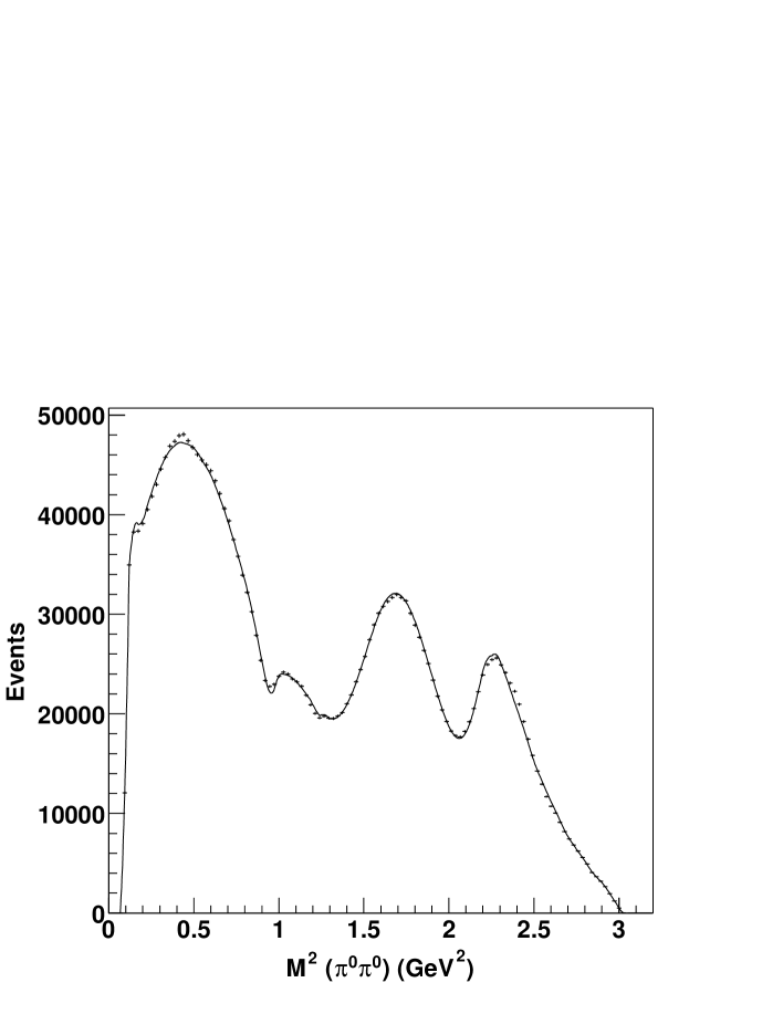
Figure 1: A mass projection of the acceptance-corrected Dalitz plot for the $p\bar{p}$ annihilation into $\pi^{0}\pi^{0}\pi^{0}$ in liquid $H_{2}$. The curve corresponds to the fit in Solution II-2.

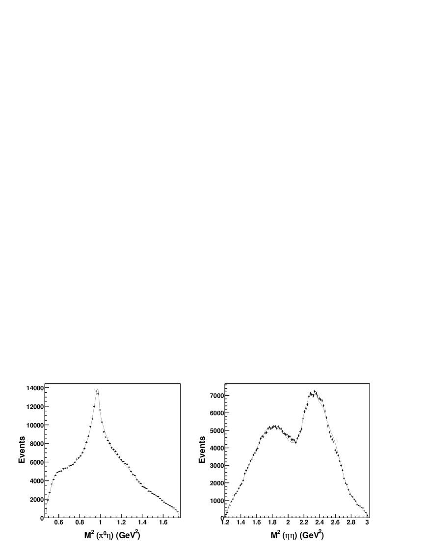
Figure 2: Mass projections of the acceptance-corrected Dalitz plot for the $p\bar{p}$ annihilation into $\pi^{0}\eta\eta$ in liquid $H_{2}$. Curves correspond to the fit in Solution II-2.

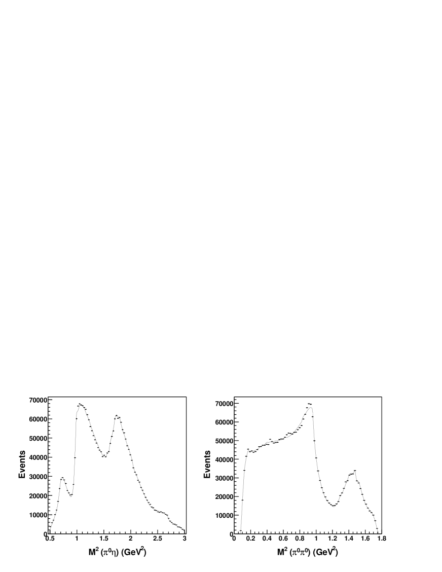
Figure 3: Mass projections of the acceptance-corrected Dalitz plot for the $p\bar{p}$ annihilation into $\pi^{0}\pi^{0}\eta$ in liquid $H_{2}$. Curves correspond to the fit in Solution II-2.

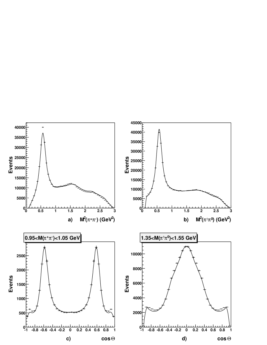
Figure 4: a,b) Mass projections of the acceptance-corrected Dalitz plot for the $p\bar{p}$ annihilation into $\pi^{+}\pi^{0}\pi^{-}$ in liquid $H_{2}$, c) the angle distribution between charged and neutral pions in c.m.s. of $\pi^{+}\pi^{-}$ system taken at masses between 0.95 and 1.05 GeV, d) the angle distribution between charged pions in c.m.s. of $\pi^{\pm}\pi^{0}$ system taken at masses between 1.35 and 1.55 GeV. Figure 4d shows the event distribution along the band with the production of $\rho(1450)$.

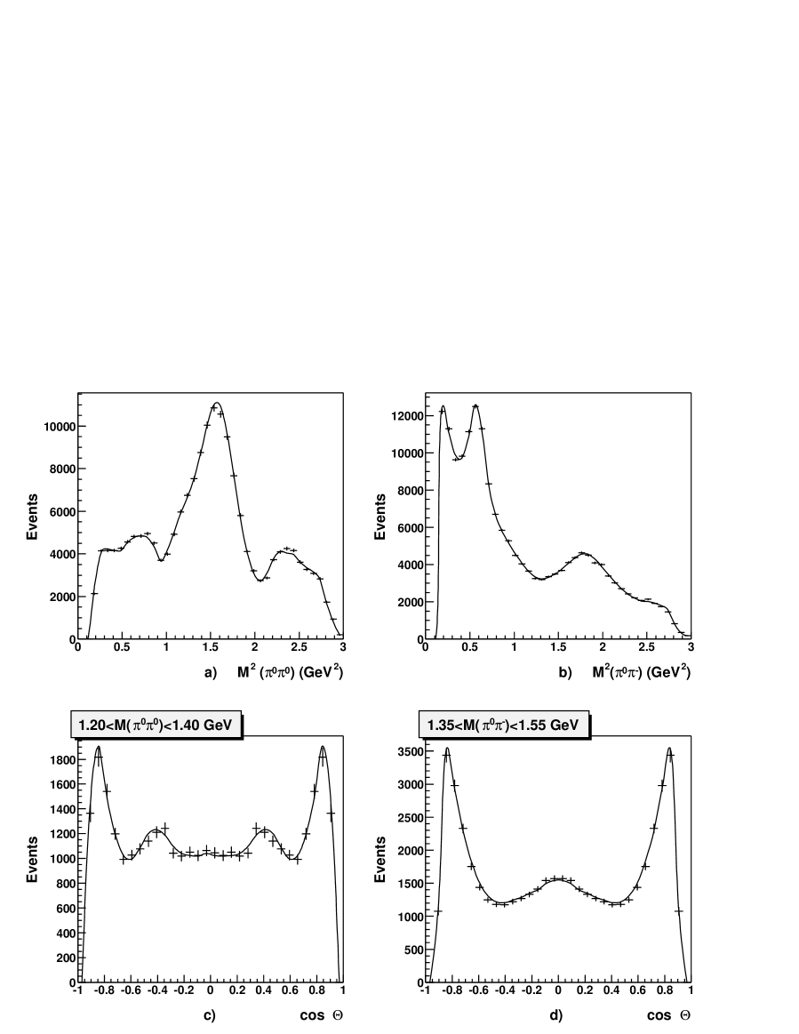
Figure 5: a,b) Mass projections of the acceptance-corrected Dalitz plot for the $p\bar{p}$ annihilation into $\pi^{0}\pi^{0}\pi^{-}$ in liquid $D_{2}$, c) the angle distribution between charged and neutral pions in c.m.s. of $\pi^{0}\pi^{0}$ system taken at masses between 1.20 and 1.40 GeV, d) the angle distribution between neutral pions in c.m.s. of $\pi^{0}\pi^{-}$ system taken at masses between 1.35 and 1.55 GeV

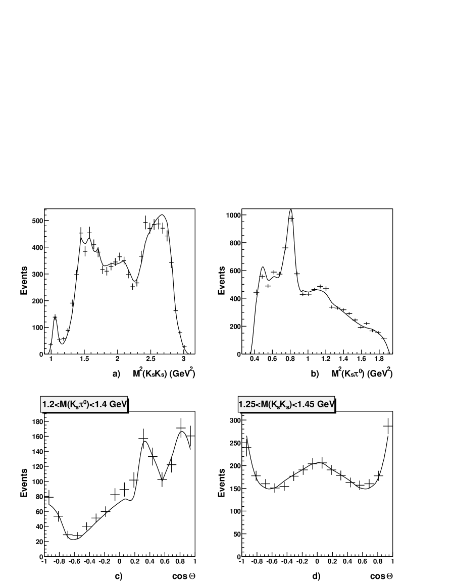
Figure 7: a,b) Mass projections of the acceptance-corrected Dalitz plot for the $p\bar{p}$ annihilation into $K_{S}K_{S}\pi^{0}$ in liquid $H_{2}$, c) the angle distribution between kaons in c.m.s. of $K_{S}\pi^{0}$ system taken at masses between 1.20 and 1.40 GeV, d) an angle distribution between kaon pion in c.m.s. of $K_{S}K_{S}$ system taken at masses between 1.25 and 1.45 GeV.

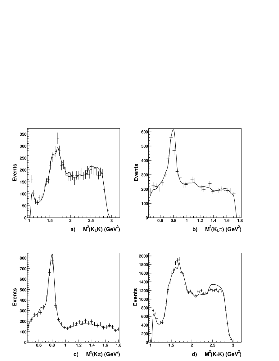
Figure 9: a,b,c) Mass projections of the acceptance-corrected Dalitz plot for the $p\bar{p}$ annihilation into $K_{L}K^{-}\pi^{+}$ ($K_{L}K^{+}\pi^{-}$) in liquid $H_{2}$, d) $K_{S}K$ mass projection of the acceptance corrected Dalitz plot for the $p\bar{p}$ annihilation into $K_{S}K^{-}\pi^{+}$. This reaction has some problems with acceptance correction and was not used in the analysis. The full curve corresponds to the fit of $\bar{p}p\to K_{L}K^{-}\pi^{+}$ reaction normalized to the number of $K_{S}K^{-}\pi^{+}$ events.

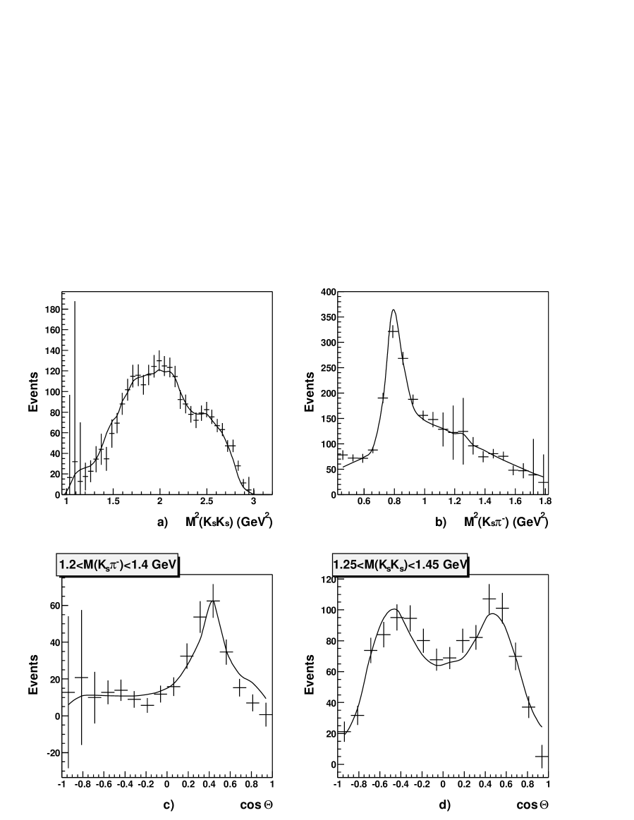
Figure 10: a,b) Mass projections of the acceptance-corrected Dalitz plot for the $p\bar{p}$ annihilation into $K_{S}K_{S}\pi^{-}$ in liquid $D_{2}$, c) the angle distribution between kaons in c.m.s. of $K_{S}\pi^{-}$ system taken at masses between 1.20 and 1.40 GeV, d) the angle distribution between kaon and pion in c.m.s. of $K_{S}K_{S}$ system taken at masses between 1.25 and 1.45 GeV.

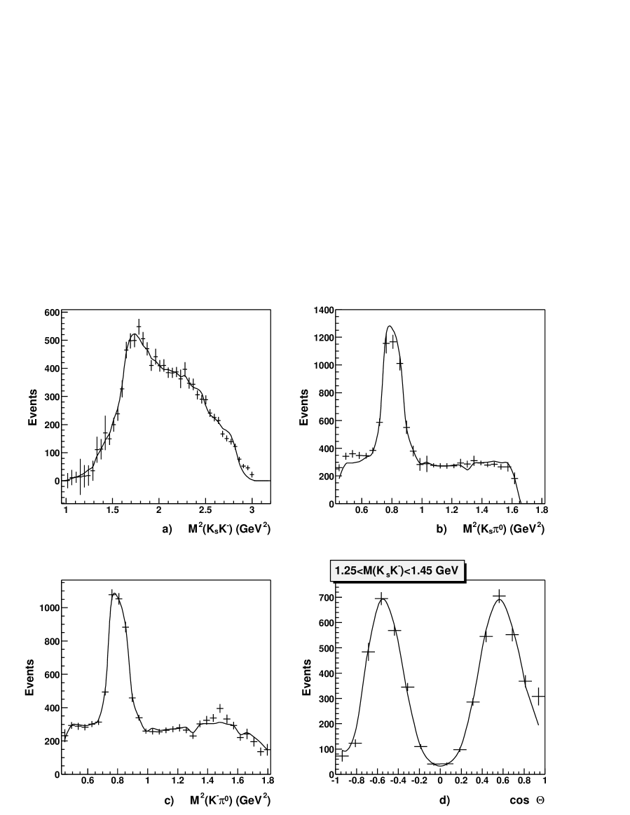
Figure 11: a,b,c) Mass projections of the acceptance-corrected Dalitz plot for the $p\bar{p}$ annihilation into $K_{S}K^{-}\pi^{0}$ in liquid $D_{2}$, d) the angle distribution between $K_{S}$ and $\pi^{0}$ in c.m.s. of $K_{S}K^{-}$ system taken at masses between 1.25 and 1.45 GeV.

Figures 1-11 demonstrate the two-meson spectra and angle distributions for the reactions $p\bar{p}\to three\;mesons$ and $n\bar{p}\to three\;mesons$. The scattering amplitudes $\pi\pi\to\pi\pi$, $\pi\pi\to\eta\eta$, and so on, are restored on the same level of accuracy as in [11], and we do not show them.

In Figs. 1, 2, 3 one can see the $M^{2}_{\pi^{0}\pi^{0}}$, $M^{2}_{\eta\pi^{0}}$, $M^{2}_{\eta\eta}$ distributions in the reactions $p\bar{p}(liquid\,H_{2})\to\pi^{0}\pi^{0}\pi^{0}\;\pi^{0}\eta\eta,\;\pi^{0}\pi^{0}\eta$. The Dalitz-plots for these reactions were the corner-stones for the $K$-matrix fits to the $00^{++}$ wave at the early stage of our study [8, 9]: Figs 1, 2, 3 demonstrate the level of accuracy of the present fit. Figure 4 shows similar mass distributions in the reaction $p\bar{p}(liquid\,H_{2})\to\pi^{+}\pi^{0}\pi^{-}$.

Figures 5 and 6 demonstrate the distributions for the reactions $n\bar{p}(liquid\,D_{2})\to\pi^{0}\pi^{0}\pi^{-}$, $\pi^{-}\pi^{-}\pi^{+}$. The angle distributions stand for bands with the production of $f_{2}(1285)+f_{0}(1300)$ (Fig. 5c) and $\rho(1450)$ (Figs. 5d, 6d). In connection with the discussion of a possible resonance structure in the $I=2$ channel, we show in Fig. 6c the angle distribution along the band $M_{\pi^{-}\pi^{-}}\sim 1300$ MeV (recall that resonance states with $I=2$ are not included into our fit).

In Figs. 7 and 8, one can see the mass and angle distributions in the reactions $p\bar{p}(liquid\,H_{2})\to K_{S}K_{S}\pi^{0},K^{+}K^{-}\pi^{0}$ (parameters for $a_{0}^{(bare)}$ and $K_{0}^{(bare)}$ have been fixed, correspondingly, in [11] and [43] ($K$-matrix re-analysys of the SLAC-NAGO-CINC-INUS data [46] for $K\pi\to K\pi$). Angle distributions in Figs. 7d and 8d are selected for the demonstration, in connection with the discussed possibility for the $a_{0}$-resonance to exist in the region $\sim 1300$ MeV (in the fit performed in [11], the $a_{0}$-state had not been found in the mass region $\sim 1300$ MeV).

In Fig. 9, the distributions in the reactions $p\bar{p}(liquid\,H_{2})\to K_{L}K^{+}\pi^{-}(K_{L}K^{-}\pi^{+}),K_{S}K^{-}\pi^{+}$ are shown. The distributions in the channel $K_{S}K^{-}\pi^{+}$ have not been fitted because of the acceptance-correction problem: the curve is the result of the fit carried out without taking account of this channel data; nevertheless, as is seen from the figure, the description is rather good.

In Figs. 10 and 11, we show distributions in the reactions $n\bar{p}(liquid\,D_{2})\to K_{S}K_{S}\pi^{-},K_{S}K^{-}\pi^{0}$. The angle distributions (Figs. 10d, 11d) are presented for the band where the production of $a_{0}(1300)$ can be seen; yet, we do not see any signal from $a_{0}(1300)$.

3.1 Bare $f_{0}$-states and resonances

In the $K$-matrix analysis of the $00^{++}$-wave, five bare states have been found, see Tables 2, 3 and 4. The bare states can be classified as nonet partners of the $q\bar{q}$ multiplets $1^{3}P_{0}$ and $2^{3}P_{0}$ or a scalar glueball. The $K$-matrix solutions give us two variants for the glueball definition: either it is a bare state with the mass near 1250 MeV, or it is located near 1600 MeV.

After having imposed the constrains (23) and (24), we found the following variants for the nonet classification.

Solution I:

$f_{0}^{\rm bare}(700\pm 100)$ and $f_{0}^{\rm bare}(1245\pm 40)$ are $1^{3}P_{0}$ nonet partners with $\varphi[f_{0}^{\rm bare}(700)]=-70^{\circ}\pm 10^{\circ}$ and $\varphi[f_{0}^{\rm bare}(1245)]=20^{\circ}\pm 10^{\circ}$.
For members of the $2^{3}P_{0}$ nonet, there are two variants:
1) either $f_{0}^{\rm bare}(1220\pm 40)$ and $f_{0}^{\rm bare}(1750\pm 30)$ are $2^{3}P_{0}$ nonet partners, with $\varphi[f_{0}^{\rm bare}(1220)]=33^{\circ}\pm 8^{\circ}$ and $\varphi[f_{0}^{\rm bare}(1750)]=60^{\circ}\pm 10^{\circ}$, while $f_{0}^{\rm bare}(1630\pm 40)$ is the glueball, with $\varphi[f_{0}^{\rm bare}(1630)]=27^{\circ}\pm 10^{\circ}$; or
2) $f_{0}^{\rm bare}(1630\pm 40)$ and $f_{0}^{\rm bare}(1750\pm 30)$ are $2^{3}P_{0}$ nonet partners, and $f_{0}^{\rm bare}(1220\pm 40)$ is the glueball.

Solution II-1:

$f_{0}^{\rm bare}(670\pm 100)$ and $f_{0}^{\rm bare}(1215\pm 40)$ are $1^{3}P_{0}$ nonet partners with $\varphi[f_{0}^{\rm bare}(670)]=-65^{\circ}\pm 10^{\circ}$ and $\varphi[f_{0}^{\rm bare}(1215)]=15^{\circ}\pm 10^{\circ}$;
$f_{0}^{\rm bare}(1560\pm 40)$ and $f_{0}^{\rm bare}(1830\pm 40)$ are $2^{3}P_{0}$ nonet partners with $\varphi[f_{0}^{\rm bare}(1560)]=15^{\circ}\pm 10^{\circ}$ and $\varphi[f_{0}^{\rm bare}(1830)]=-80^{\circ}\pm 10^{\circ}$,
$f_{0}^{\rm bare}(1220)$ is the glueball, $\varphi[f_{0}^{\rm bare}(1220)]=40^{\circ}\pm 10^{\circ}$.

Solution II-2:

$f_{0}^{\rm bare}(700\pm 100)$ and $f_{0}^{\rm bare}(1220\pm 40)$ are $1^{3}P_{0}$ nonet partners with $\varphi[f_{0}^{\rm bare}(700)]=-70^{\circ}\pm 10^{\circ}$ and $\varphi[f_{0}^{\rm bare}(1220)]=15^{\circ}\pm 10^{\circ}$.
In this Solution there are two variants for the $2^{3}P_{0}$ nonet:
1) either $f_{0}^{\rm bare}(1230\pm 30)$ and $f_{0}^{\rm bare}(1830\pm 40)$ are $2^{3}P_{0}$ nonet partners with $\varphi[f_{0}^{\rm bare}(1230)]=43^{\circ}\pm 8^{\circ}$ and $\varphi[f_{0}^{\rm bare}(1830)]=-60^{\circ}\pm 10^{\circ}$,
$f_{0}^{\rm bare}(1560\pm 30)$ is the glueball, with $\varphi[f_{0}^{\rm bare}(1560)]=15^{\circ}\pm 10^{\circ}$, or
2) $f_{0}^{\rm bare}(1560\pm 30)$ and $f_{0}^{\rm bare}(1830\pm 40)$ are nonet partners and $f_{0}^{\rm bare}(1230)$ is the glueball.

Tables 2, 3 and 4 present parameters which correspond to these three Solutions.

Table 2:

Masses, coupling constants (in GeV) and mixing angles (in degrees) for the $f_{0}^{\rm bare}$-resonances for Solution I. The errors reflect the boundaries for a satisfactory description of the data. The sheet II is under the $\pi\pi$ and $4\pi$ cuts; the sheet IV is under the $\pi\pi$, $4\pi$, $K\bar{K}$ and $\eta\eta$ cuts; the sheet V is under the $\pi\pi$, $4\pi$, $K\bar{K}$, $\eta\eta$ and $\eta\eta^{\prime}$ cuts.
 
Solution I $\alpha=1$ $\alpha=2$ $\alpha=3$ $\alpha=4$ $\alpha=5$ M $0.650^{+.120}_{-.050}$ $1.245^{+.040}_{-.030}$ $1.220^{+.030}_{-.030}$ $1.630^{+.030}_{-.020}$ $1.750^{+.040}_{-.040}$ $g^{(\alpha)}$ $0.940^{+.80}_{-.100}$ $1.050^{+.080}_{-.080}$ $0.680^{+.060}_{-.060}$ $0.680^{+.060}_{-.060}$ $0.790^{+.080}_{-.080}$ $g_{5}^{(\alpha)}$ 0 0 $0.960^{+.100}_{-.150}$ $0.900^{+.070}_{-.150}$ $0.280^{+.100}_{-.100}$ $\varphi_{\alpha}(deg)$ -(72${}^{+5}_{-10}$) 18.0${}^{+8}_{-8}$ 33${}^{+8}_{-8}$ 27${}^{+10}_{-10}$ -59${}^{+10}_{-10}$ $a=\pi\pi$ $a=K\bar{K}$ $a=\eta\eta$ $a=\eta\eta^{\prime}$ $a=4\pi$ $f_{1a}$ $-0.050^{+.100}_{-.100}$ $0.250^{+.100}_{-.100}$ $0.440^{+.100}_{-.100}$ $0.320^{+.100}_{-.100}$ $-0.540^{+.100}_{-.100}$ $f_{ba}=0$ $b=2,3,4,5$ Pole position sheet II $1.031^{+.008}_{-.008}$ $-i(0.032^{+.008}_{-.008})$ sheet IV $1.306^{+.020}_{-.020}$ $1.489^{+.008}_{-.004}$ $1.480^{+.100}_{-.150}$ $-i(0.147^{+.015}_{-.025})$ $-i(0.051^{+.005}_{-.005})$ $-i(1.030^{+.080}_{-.170})$ sheet V $1.732^{+.015}_{-.015}$ $-i(0.072^{+.015}_{-.015})$

Table 3:

Masses, coupling constants (in GeV) and mixing angles (in degrees) for the $f_{0}^{\rm bare}$-resonances for Solution II-1. The errors reflect the boundaries for a satisfactory description of the data. The sheet II is under the $\pi\pi$ and $4\pi$ cuts; the sheet IV is under the $\pi\pi$, $4\pi$, $K\bar{K}$ and $\eta\eta$ cuts; the sheet V is under the $\pi\pi$, $4\pi$, $K\bar{K}$, $\eta\eta$ and $\eta\eta^{\prime}$ cuts.
 
Solution II-1 $\alpha=1$ $\alpha=2$ $\alpha=3$ $\alpha=4$ $\alpha=5$ M $0.670^{+.100}_{-.100}$ $1.215^{+.40}_{-.040}$ $1.220^{+.015}_{-.030}$ $1.560^{+.030}_{-.040}$ $1.830^{+.030}_{-.050}$ $g^{(\alpha)}$ $0.990^{+.080}_{-.120}$ $1.100^{+.080}_{-.100}$ $0.670^{+.100}_{-.120}$ $0.500^{+.060}_{-.060}$ $0.410^{+.060}_{-.060}$ $g_{5}^{(\alpha)}$ 0 0 $0.870^{+.100}_{-.100}$ $0.600^{+.100}_{-.100}$ $-0.850^{+.080}_{-.080}$ $\varphi_{\alpha}(deg)$ -(66${}^{+8}_{-10}$) 13${}^{+8}_{-5}$ 40${}^{+12}_{-12}$ 15${}^{+08}_{-15}$ -80${}^{+10}_{-10}$ $a=\pi\pi$ $a=K\bar{K}$ $a=\eta\eta$ $a=\eta\eta^{\prime}$ $a=4\pi$ $f_{1a}$ $0.050^{+.100}_{-.100}$ $0.100^{+.080}_{-.080}$ $0.360^{+.100}_{-.100}$ $0.320^{+.100}_{-.100}$ $-0.350^{+.060}_{-.060}$ $f_{ba}=0$ $b=2,3,4,5$ Pole position sheet II $1.020^{+.008}_{-.008}$ $-i(0.035^{+.008}_{-.008})$ sheet IV $1.320^{+.020}_{-.020}$ $1.485^{+.005}_{-.006}$ $1.530^{+.150}_{-.100}$ $-i(0.130^{+.015}_{-.025})$ $-i(0.055^{+.008}_{-.008})$ $-i(0.900^{+.100}_{-.200})$ sheet V $1.785^{+.015}_{-.015}$ $-i(0.135^{+.025}_{-.010})$

Table 4:

Masses, coupling constants (in GeV) and mixing angles (in degrees) for the $f_{0}^{\rm bare}$-resonances for Solution II-2. The errors reflect the boundaries for a satisfactory description of the data. The sheet II is under the $\pi\pi$ and $4\pi$ cuts; the sheet IV is under the $\pi\pi$, $4\pi$, $K\bar{K}$ and $\eta\eta$ cuts; the sheet V is under the $\pi\pi$, $4\pi$, $K\bar{K}$, $\eta\eta$ and $\eta\eta^{\prime}$ cuts.
 
Solution II-2 $\alpha=1$ $\alpha=2$ $\alpha=3$ $\alpha=4$ $\alpha=5$ M $0.650^{+.120}_{-.050}$ $1.220^{+.040}_{-.030}$ $1.230^{+.030}_{-.030}$ $1.560^{+.030}_{-.020}$ $1.830^{+.040}_{-.040}$ $g^{(\alpha)}$ $1.050^{+.80}_{-.100}$ $0.980^{+.080}_{-.080}$ $0.470^{+.050}_{-.050}$ $0.420^{+.040}_{-.040}$ $0.420^{+.050}_{-.050}$ $g_{5}^{(\alpha)}$ 0 0 $0.870^{+.100}_{-.100}$ $0.560^{+.070}_{-.070}$ $-0.780^{+.070}_{-.070}$ $\varphi_{\alpha}(deg)$ -(68${}^{+3}_{-15}$) 14${}^{+8}_{-8}$ 43${}^{+8}_{-8}$ 15${}^{+10}_{-10}$ -55${}^{+10}_{-10}$ $a=\pi\pi$ $a=K\bar{K}$ $a=\eta\eta$ $a=\eta\eta^{\prime}$ $a=4\pi$ $f_{1a}$ $0.260^{+.100}_{-.100}$ $0.100^{+.100}_{-.100}$ $0.260^{+.100}_{-.100}$ $0.260^{+.100}_{-.100}$ $-0.140^{+.060}_{-.060}$ $f_{ba}=0$ $b=2,3,4,5$ Pole position sheet II $1.020^{+.008}_{-.008}$ $-i(0.035^{+.008}_{-.008})$ sheet IV $1.325^{+.020}_{-.030}$ $1.490^{+.010}_{-.010}$ $1.450^{+.150}_{-.100}$ $-i(0.170^{+.020}_{-.040})$ $-i(0.060^{+.005}_{-.005})$ $-i(0.800^{+.100}_{-.150})$ sheet V $1.740^{+.020}_{-.020}$ $-i(0.160^{+.025}_{-.010})$

3.2 GAMS and E852 data on the $\pi\pi$ $S$-wave production $\pi^{-}p\to(\pi\pi)_{S}\;n$ at moderate momenta transferred to nucleon, $0<|t|<1.5$ (GeV/$c$)²

The formulae of Section 2.2 allow one to describe simultaneously the $\pi\pi$ spectra in the reaction $\pi^{-}p\to(\pi\pi)_{S}\,n$ at $p_{lab}=18$ GeV/c [19] and $p_{lab}=38$ GeV/c [12].

The leading $\pi$ and $a_{1}$ trajectories have rather close intercepts and slopes [33], so corresponding reggeon exchanges do not cause a change of $t$-distributions with energy. However, the experimental data definitely point to a break of similarity of the spectra: in Fig. 12 the difference of the $M_{\pi\pi}$-distributions is shown for $|t|\sim(0.3-0.4)$ (GeV/c)² where one can trace differences in spectra related to E852 and GAMS experiments. This fact definetely points to a significant contribution of daughter trajectories.

We have fitted to data [12] and [19] under a variety of assumptions on the $|t|$-exchange structure; these versions of fitting are discussed in a separate publication [32]. Here, in Figs. 13 and 14, we demonstrate typical description of the data. Figure 13 represents the $M_{\pi\pi}$ spectra of E852 Collaboration for different $|t|$-intervals, and figure 14 shows the same for GAMS group (calculated spectra refer to Solution II-2).

In Fig. 15, we show form factors for $\pi$ and $a_{1}$ exchanges, which at large $|t|$ describe effectively the multi-reggeon interactions. We show the form factors which correspond to the so-called Orear behaviour of the scattering amplitude [47] at large $|t|$ (see also [48] and references therein):

$$G^{(\alpha)}_{\pi\pi}(t)=g_{\pi\pi}\left[\exp\left(\beta_{1}^{(\alpha)}(t-m^{2}_{\pi})\right)+\Lambda(t-m^{2}_{\pi})\exp\left(-\beta_{2}^{(\alpha)}\sqrt{|t-m^{2}_{\pi}|}\right)\right]\ .$$ (25)

Another types of the behaviour of $G^{(\alpha)}_{\pi\pi}(t)$ were analysed in [32].

4 $f_{0}$-resonances: masses, decay couplings and
partial widths

The resonance masses and decay couplings are not determined directly in the fitting procedure. To calculate these quantities one needs to perform analytical continuation of the $K$-matrix amplitude into lower half-plane of the complex plane $s$. One is allowed to do it, for the $K$-matrix amplitude correctly takes into account the threshold singularities related to the $\pi\pi$, $\pi\pi\pi\pi$, $K\bar{K}$, $\eta\eta$, $\eta\eta^{\prime}$ channels which are important in the $00^{++}$-wave.

4.1 Masses of resonances

The complex masses of the resonances $f_{0}(980)$, $f_{0}(1300)$, $f_{0}(1500)$, $f_{0}(1200-1600)$ obtained in Solutions I, II-1 and II-2 do not differ strongly. Solutions I and II are essentially different in the characteristics of the $f_{0}(1750)$

For the pole positions the following values, in MeV, have been found:

$${\rm Solution\;I:} f_{0}(980) \to 1031-i\;32$$

$$f_{0}(1300) \to 1306-i\;147$$

$$f_{0}(1500) \to 1489-i\;51$$

$$f_{0}(1750) \to 1732-i\;72$$

$$f_{0}(1200-1600) \to 1480-i\;1030$$

$${\rm Solution\;II-1:} f_{0}(980) \to 1020-i\;34$$

$$f_{0}(1300) \to 1320-i\;130$$

$$f_{0}(1500) \to 1485-i\;55$$

$$f_{0}(1750) \to 1785-i\;135$$

$$f_{0}(1200-1600) \to 1530-i\;930$$

$${\rm Solution\;II-2:} f_{0}(980) \to 1020-i\;35$$

$$f_{0}(1300) \to 1325-i\;170$$

$$f_{0}(1500) \to 1490-i\;60$$

$$f_{0}(1750) \to 1740-i\;160$$

$$f_{0}(1200-1600) \to 1450-i\;800$$

We see that Solutions I and II give different magnitudes for total width of the $f_{0}(1750)$.

4.2 Decay couplings and partial widths

We determine the coupling constants and partial decay widths using the following procedure. The $00^{++}$-amplitude for the transition $a\to b$,

$$A_{a\to b}(s)\;,\qquad a,b=\pi\pi,K\bar{K},\eta\eta,\eta\eta^{\prime},\pi\pi\pi\pi,$$ (29)

is considered as a function of the invariant energy squared $s$ in the complex-$s$ plane near the pole related to the resonance $n$. In the vicinity of the pole the amplitude reads:

$$A_{a\to b}(s)=\frac{g^{(n)}_{a}g^{(n)}_{b}}{\mu^{2}_{n}-s}\;e^{i(\theta^{(n)}_{a}+\theta^{(n)}_{b})}+{\rm non-pole\;terms}\ .$$ (30)

Here $\mu_{n}$ is the resonance complex mass $\mu_{n}=M_{n}-i\Gamma_{n}/2\;$; $g^{(n)}_{a}$ and $g^{(n)}_{b}$ are the couplings for the transitions $f_{0}\to a$ and $f_{0}\to b$. In (30), the non-pole background terms are omitted.

The decay coupling constants squared, $g^{(n)\;2}_{a}$, are shown in Table 5 for $a=\pi\pi$, $K\bar{K}$, $\eta\eta$, $\eta\eta^{\prime}$, $\pi\pi\pi\pi$. The couplings are determined with the normalization of the amplitude used in Section 2: for example, we write the $\pi\pi$ scattering amplitude (30) as

$$A_{\pi\pi\to\pi\pi}(s)=(\eta^{0}_{0}\exp{(2i\delta^{0}_{0})}-1)/2i\rho_{\pi\pi}(s)\ ,$$

where $\eta^{0}_{0}$ and $\delta^{0}_{0}$ are the inelasticity parameter and phase shift for the $00^{++}$ $\pi\pi$-wave, reprectively. The coupling constants $g^{(n)\;}_{a}$ are found by calculating the residues of the amplitudes $\pi\pi\to\pi\pi$, $K\bar{K}$, $\eta\eta$, $\eta\eta^{\prime}$, $\pi\pi\pi\pi$. Also we check the factorization property for the pole terms by calculating residues for other reactions, such as $K\bar{K}\to K\bar{K}$, and so on.

The resonance $f_{0}(980)$ is located near the strong $K\bar{K}$ threshold, therefore two poles are related to $f_{0}(980)$: for example, in Solution II-2 the nearest one is on the 3rd sheet (under $\pi\pi$ and $\pi\pi\pi\pi$ cuts, at $M\simeq 1020-i35$ MeV) and a remote pole on the 4th sheet (under $\pi\pi$, $\pi\pi\pi\pi$ and $K\bar{K}$ cuts, at $M\simeq 940-i240$ MeV). Coupling constants for $f_{0}(980)$ are determined as residues of the nearest pole which is located on the 3rd sheet.

Table 5: Coupling constants squared (in GeV²) of scalar-isoscalar resonances to hadronic channels $\pi\pi$, $K\bar{K}$, $\eta\eta$, $\eta\eta^{\prime}$ and $\pi\pi\pi\pi$ for different $K$-matrix solutions.

Pole position	$\pi\pi$	$K\bar{K}$	$\eta\eta$	$\eta\eta^{\prime}$	$\pi\pi\pi\pi$	Solution
$f_{0}(980)$
$1031-i32$	0.056	0.130	0.067	–	0.004	I
$1020-i35$	0.051	0.115	0.051	–	0.003	II-1
$1020-i35$	0.054	0.117	0.139	–	0.004	II-2
$f_{0}(1300)$
$1306-i147$	0.036	0.009	0.006	0.004	0.093	I
$1320-i130$	0.038	0.003	0.005	0.012	0.109	II-1
$1325-i170$	0.053	0.003	0.007	0.013	0.226	II-2
$f_{0}(1500)$
$1489-i51$	0.014	0.006	0.003	0.001	0.038	I
$1485-i55$	0.020	0.007	0.004	0.003	0.049	II-1
$1490-i60$	0.018	0.007	0.003	0.003	0.076	II-2
$f_{0}(1750)$
$1732-i72$	0.013	0.062	0.002	0.032	0.002	I
$1785-i135$	0.066	0.003	0.007	0.033	0.080	II-1
$1740-i160$	0.089	0.002	0.009	0.035	0.168	II-2
$f_{0}(1200-1600)$
$\;1480-i1000$	0.364	0.265	0.150	0.052	0.524	I
$1530-i900$	0.325	0.235	0.086	0.015	0.474	II-1
$1450-i800$	0.179	0.204	0.046	0.005	0.686	II-2

The partial width for the decay $f_{0}\to a$ is determined as a product of the coupling constant squared, $g^{(n)\;2}_{a}$, and phase space, $\rho_{a}(s)$, averaged over the resonance density:

$$\Gamma_{a}(n)=C_{n}\int\limits_{s>s_{th}}\frac{ds}{\pi}\,\frac{g^{(n)\;2}_{a}\;\rho_{a}(s)}{(Re\;\mu^{2}_{n}-s)^{2}+({\rm Im}\,\mu^{2}_{n})^{2}}\ .$$ (31)

The resonance density factor, $\left[(Re\;\mu^{2}_{n}-s)^{2}+({\rm Im}\,\mu^{2}_{n})^{2}\right]^{-1}$, guarantees rapid convergence of the integral (31). The normalization constant $C_{n}$ is determined by the requirement that the sum of all hadronic partial widths is equal to the total width of the resonance:

$$\Gamma(n)=\sum\limits_{a}\Gamma_{a}(n)\ .$$ (32)

In Table 6 we show the values of partial widths for the resonances $f_{0}(980)$, $f_{0}(1300)$, $f_{0}(1500)$, $f_{0}(1750)$. Partial widths for $f_{0}(1300)$, $f_{0}(1500)$, $f_{0}(1750)$ are calculated within standard formulae for the Breit-Wigner resonances (31).

Table 6: Partial widths of scalar-isoscalar resonances (in MeV) in hadronic channels $\pi\pi$, $K\bar{K}$, $\eta\eta$, $\eta\eta^{\prime}$ and $\pi\pi\pi\pi$ for different $K$-matrix solutions.

	$\pi\pi$	$K\bar{K}$	$\eta\eta$	$\eta\eta^{\prime}$	$\pi\pi\pi\pi$	$\Gamma_{tot}/2$	Solution
$f_{0}(980)$	52	10	–	–	2	32	I
	57	9	–	–	2	34	II-1
	58	10	–	–	2	35	II-2
$f_{0}(1300)$	77	14	7	–	196	147	I
	66	4	4	–	186	130	II-1
	63	3	5	–	269	170	II-2
$f_{0}(1500)$	23	6	3	0.0	70	51	I
	25	7	3	0.1	75	55	II-1
	22	6	2	0.1	88	59	II-2
$f_{0}(1750)$	31	96	5	7	5	72	I
	114	3	8	7	138	135	II-1
	103	1	8	4	204	160	II-2

Because of a strong $K\bar{K}$ threshold near the pole, the resonance term for $f_{0}(980)$ should be used not as the Breit-Wigner amplitude but in a more complicated form. Instead of the Breit-Wigner pole term $R^{(ab)}_{n}=g^{(n)}_{a}g^{(n)}_{b}/(\mu^{2}_{n}-s)$ entering equation (30), the following resonance amplitudes can be written for the $\pi\pi\to\pi\pi$ and $K\bar{K}\to K\bar{K}$ transitions near $f_{0}(980)$ [49]:

$$R^{(\pi\pi,\pi\pi)}_{f_{0}(980)}=\left[G^{2}+i\frac{\sqrt{s-4m^{2}_{K}}}{m_{0}}(2GG_{K\bar{K}}f+f^{2}(m^{2}_{0}-s))\right]\,\frac{1}{D}\ ,$$ (33)

$$R^{(K\bar{K},K\bar{K})}_{f_{0}(980)}=\left[G^{2}_{K\bar{K}}+i(2GG_{K\bar{K}}f+f^{2}(m^{2}_{0}-s))\right]\,\frac{1}{D}\ ,$$

where

$$D=m^{2}_{0}-s-iG^{2}-i\frac{\sqrt{s-4m^{2}_{K}}}{m_{0}}\left[G^{2}_{K\bar{K}}+i(2GG_{K\bar{K}}f+f^{2}(m^{2}_{0}-s))\right]\ .$$ (34)

Here $m_{0}$ is the input mass of $f_{0}(980)$; $G$ and $G_{K\bar{K}}$ are coupling constants to pion and kaon channels. The dimensionless constant $f$ stands for the prompt transition $K\bar{K}\to\pi\pi$: the value $f/m_{0}$ is the ”transition length” which is analogous to the scattering length of the low-energy hadronic interaction. The constants $m_{0}$, $G$, $G_{K\bar{K}}$, $f$ are parameters which are to be chosen to reproduce the $f_{0}(980)$ charactristics. Equations (33) and (34) are written for $s>4m^{2}_{K}$, at $s<4m^{2}_{K}$ one needs to replace $\sqrt{s-4m^{2}_{K}}\to i\sqrt{4m^{2}_{K}-s}$.

In [49], two sets of parameters were obtained, with sufficiently correct values for the $f_{0}(980)$ pole position and couplings. They are equal (in GeV) to:

$$Solution\,A:\quad m_{0}=1.000\ ,\,f=0.516\ ,\,G=0.386\ ,\,G_{K\bar{K}}=0.447\ ,$$

$$Solution\,B:\quad m_{0}=0.952\ ,\,f=-0.478\ ,\,G=0.257\ ,\,G_{K\bar{K}}=0.388\ .$$ (35)

Partial widths of $f_{0}(980)$ are calculated with the expression similar to (31), with the replacement of the integrand denominator as follows:

$$({\rm Re}\,\mu_{n}^{2}-s)^{2}+({\rm Im}\,\mu_{n}^{2})^{2}\to|D|^{2}.$$ (36)

For both sets of parameters (35) the calculated partial widths are close to each other. The values of partial widths for $f_{0}(980)$ averaged over Solutions $A$ and $B$ are presented in Table 6.

The total hadron width of $f_{0}(980)$ is defined in the same way as for the other $f_{0}$-mesons, namely, by using the position of pole in the complex-$M$ plane: the imaginary part of the mass is equal to a half-width of the resonance. For the Breit–Wigner resonance this definition is in accordance with what is observed from resonance spectrum (provided there is no interference with the background). If the resonance is located in the vicinity of a strong threshold, the visible resonance width differs significantly from that given by pole position.

The results of our calculations of partial decay widths are presented below, the magnitudes are in MeV. In the brackets we demonstrate the values obtained in [49] on the basis of previous analysis [11]:

Resonance	$\Gamma_{\pi\pi}$	$\Gamma_{K\bar{K}}$	$\Gamma_{\eta\eta}$	$\Gamma_{\eta\eta^{\prime}}$	$\Gamma_{\pi\pi\pi\pi}$	$\Gamma_{tot}/2$	Solution
$f_{0}(980):$	$55\pm 5$	$10\pm 1$	–	–	$2\pm 1$	$34\pm 5$	I,II
	$(64\pm 8)$	$(12\pm 1)$	–	–	$(4\pm 2)$	$(40\pm 5)$	[11, 49]
$f_{0}(1300):$	$66\pm 10$	$6\pm 4$	$5\pm 2$	–	$230\pm 50$	$150\pm 20$	I,II
	$(46\pm 12)$	$(5\pm 3)$	$(4\pm 2)$	–	$(171\pm 10)$	$(113\pm 10)$	[11, 49]
$f_{0}(1500):$	$23\pm 5$	$6\pm 2$	$3\pm 1$	$0.1\pm 0.1$	$80\pm 10$	$55\pm 5$	I,II
	$(37\pm 2)$	$(7\pm 2)$	$(4\pm 1)$	$(0.2\pm 0.1)$	$(79\pm 6)$	$(62\pm 3)$	[11, 49]
$f_{0}(1750):$	$30\pm 5$	$100\pm 10$	$5\pm 3$	$7\pm 3$	$5\pm 5$	$70\pm 20$	I
	$105\pm 10$	$2\pm 1$	$8\pm 1$	$5\pm 3$	$170\pm 40$	$150\pm 25$	II
	$(74^{+15}_{-30})$	$(11^{+17}_{-9})$	$(7\pm 1)$	$(3\pm 1)$	$(91^{+30}_{-60})$	$(93^{+20}_{-40})$	[11, 49]

(37)

In Solutions I and II, partial widths for $f_{0}(980)$, $f_{0}(1300)$, $f_{0}(1500)$ are agreeably coincide but for $f_{0}(1750)$ the decay characteristics are different. So we present separately the $f_{0}(1750)$ partial widths for both Solutions, I and II.

5 Classification of scalar resonances

The $K$-matrix approach works ingenuously with the bare states thus directly providing the $q\bar{q}$-classification for these states. Concerning the resonances, the classifications of the $a_{0}$ and $K_{0}$ mesons in terms of bare states and real resonances are similar, while $f_{0}$ mesons give us an opposite case: the matter is that there is an exotic state, gluonium, in the region under consideration, whose mixing with $q\bar{q}$ state is not forbidden by the $1/N$ expansion rules (for more detail see [5, 42]).

In the present Section, on the basis of the values for couplings to channels $\pi\pi$, $K\bar{K}$, $\eta\eta$, $\eta\eta^{\prime}$ calculated in Section 4, we analyse the quark-gluonium content of resonances $f_{0}(980)$, $f_{0}(1300)$, $f_{0}(1500)$, $f_{0}(1750)$ and the broad state $f_{0}(1200-1600)$.

5.1 Overlapping of the $f_{0}$-resonances in the mass region 1200–1700 MeV: accumulation of widths of the $q\bar{q}$ states by the glueball

The existence of the broad resonance is not an eventual phenomenon: it originated due to the mixing of states in the decay processes, namely, transitions $f_{0}(m_{1})\to real\;mesons\;\to f_{0}(m_{2})$. These transitions result in a specific phenomenon, that is, when several resonances overlap, one of them accumulates the widths of neighbouring resonances and transforms into the broad state.

This phenomenon had been observed in [8, 9] for scalar-isoscalar states, and the following scheme has been suggested in [42, 50]: the broad state $f_{0}(1200-1600)$ is the descendant of the pure glueball which being in the neighbourhood of $q\bar{q}$ states accumulated their widths and transformed into the mixture of gluonium and $q\bar{q}$ states. In [42], this idea had been modelled for four resonances $f_{0}(1300)$, $f_{0}(1500)$, $f_{0}(1200-1600)$ and $f_{0}(1750)$, by using the language of the quark-antiquark and two-gluon states, $q\bar{q}$ and $gg$: the decay processes were considered as the transitions $f_{0}\to q\bar{q},gg$, correspondingly; the same processes are responsible for the mixing of resonances. In this model, the gluonium component is mainly dispersed over three resonances, $f_{0}(1300)$, $f_{0}(1500)$, $f_{0}(1200-1600)$, so every state is a mixture of $q\bar{q}$ and $gg$ components, with roughly equal percentage of gluonium (about 30-40%).

Accumulation of widths of overlapping resonances by one of them is a well-known effect in nuclear physics [51, 52, 53]. In meson physics this phenomenon can play rather important role, in particular for exotic states which are beyond the $q\bar{q}$ systematics. Indeed, being among $q\bar{q}$ resonances, the exotic state creates a group of overlapping resonances. The exotic state, which is not orthogonal to its neighbours, after accumulating the ”excess” of widths turns into the broad one. This broad resonance should be accompanied by narrow states which are the descendants of states from which the widths have been taken off. In this way, the existence of a broad resonance accompanied by narrow ones may be a signature of exotics. This possibility, in context of searching for exotic states, was discussed in [10, 54].

The broad state may be one of the components which form the confinement barrier: the broad states, after accumulating the widths of neighbouring resonances, play for these latter the role of locking states. Evaluation of the mean radii squared of the broad state $f_{0}(1200-1600)$ and its neighbouring resonances argues in favour of this idea, for the radius of $f_{0}(1200-1600)$ is significantly larger than that of $f_{0}(980)$ and $f_{0}(1300)$ [10, 55], thus making $f_{0}(1200-1600)$ to be the locking state. The data on the $t$-dependence in the reaction $\pi^{-}p\to(\pi\pi)_{S}\,n$ at $p_{beam}=18$ (GeV/c)² [19] also support this idea, for the signal from the broad state (background in the spectra) falls with the increase of $|t|$ much quicker than that of the $f_{0}(980)$ and $f_{0}(1300)$.

The $K$-matrix solutions obtained here (Section 3.1) give us two variants for the transformation of bare states into real resonances coming after the onset of the decay channels. They are as follows:

$$\begin{array}[]{cl}f_{0}^{bare}(700)\pm 100)&\to\;f_{0}(980)\ ,\\ f_{0}^{bare}(1220\pm 40)&\to\;f_{0}(1300)\ ,\\ f_{0}^{bare}(1230\pm 40)&\to\;{\rm broad\,state}\,f_{0}(1200-1600)\ ,\\ f_{0}^{bare}(1580\pm 40)&\to\;f_{0}(1500)\ ,\\ f_{0}^{bare}(1800\pm 40)&\to\;f_{0}(1750)\ .\end{array}$$ (43)

and

$$\begin{array}[]{cl}f_{0}^{bare}(700)\pm 100)&\to\;f_{0}(980)\ ,\\ f_{0}^{bare}(1220\pm 40)&\to\;f_{0}(1300)\ ,\\ f_{0}^{bare}(1230\pm 40)&\to\;f_{0}(1500)\ ,\\ f_{0}^{bare}(1580\pm 40)&\to\;{\rm broad\,state}\,f_{0}(1200-1600)\ ,\\ f_{0}^{bare}(1800\pm 40)&\to\;f_{0}(1750)\ .\end{array}$$ (49)

The evolution of bare states into real resonances is illustrated by Fig. 16: the shifts of amplitude poles in the complex-$M$ plane correspond to a gradual onset of the decay channels. Technically it is done by replacing the phase spaces $\rho_{a}$ for $a=\pi\pi$, $\pi\pi\pi\pi$, $K\bar{K}$, $\eta\eta$, $\eta\eta^{\prime}$ in the $K$-matrix amplitude as follows: $\rho_{a}\to\xi\rho_{a}$, where the parameter $\xi$ runs in the interval $0\leq\xi\leq 1$. At $\xi\to 0$ one has bare states, while the limit $\xi\to 1$ gives us the positions of real resonances.

5.2 Hadronic decays and evaluation of the quark-gluonium content of scalar-isoscalar resonances

Here, on the basis of the quark combinatorics for the decay coupling constants, we analyse quark-gluonium content of resonances $f_{0}(980),f_{0}(1300),f_{0}(1500),f_{0}(1750)$ and the broad state $f_{0}(1200-1600)$.

The comparison of Tables 2, 3, 4 with Table 5 demonstrates a strong change of couplings during the evolution from bare states to real resonances; the same type of strong deviation of couplings has been observed before, for previous $K$-matrix solutions, see [56]. Note that the change occurs not only in absolute values of couplings but in relative magnitudes as well that means the change of the quark-antiquark content of states in the evolution caused by the decay onset.

Let us look at the proportion of $s\bar{s}$, $n\bar{n}$ and gluonium components given by quark-combinatorics relations (22) for the studied resonances. The coupling constants squared for $f_{0}\to\pi\pi$, $K\bar{K}$, $\eta\eta$, $\eta\eta^{\prime}$ in (22) are expressed as a sum of two terms which correspond to transitions of quarkonium and gluonium components into two pseudoscalar mesons.

First, let us find the mean value of mixing angle, $\langle\varphi\rangle$, for the $n\bar{n}$/$s\bar{s}$ components in the intermediate state. Because of the two-stage mechanism of the gluonium decay $gluonium\to quark-antiquark\;pair\to two\;mesons$ (see [5] and Appendix C), we determine $\langle\varphi\rangle$ in the intermediate state as follows:

$$f_{0}\to{\rm gluonium}+q\bar{q}\to n\bar{n}\cos\langle\varphi\rangle+s\bar{s}\sin\langle\varphi\rangle\to{\rm two\;mesons}.$$ (50)

So, $\langle\varphi\rangle$ is the angle corresponding to the coupling constants squared (22) at $G=0$.

Based on the values of couplings given in Table 5, we have found the following values of $\langle\varphi\rangle$ and $\lambda$.
Solution I:

$$f_{0}(980): \quad\langle\varphi\rangle\simeq-68^{\circ}\ , \lambda\simeq 0.5-1.0\ ,$$ (51)

$$f_{0}(1300): \quad\langle\varphi\rangle\simeq(-3^{\circ})-4^{\circ}\ , \lambda\simeq 0.5-0.9\ ,$$

$${\rm Broad\;\;state\;\;}f_{0}(1200-1600): \quad\langle\varphi\rangle\simeq 27^{\circ}\ , \lambda\simeq 0.54\ ,$$

$$f_{0}(1500): \quad\langle\varphi\rangle\simeq 12^{\circ}-19^{\circ}\ , \lambda\simeq 0.5-1.0\ ,$$

$$f_{0}(1750): \quad\langle\varphi\rangle\simeq-72^{\circ}\ , \lambda\simeq 0.5-0.7\ ,$$

Solution II-1:

$$f_{0}(980): \quad\langle\varphi\rangle\simeq-67^{\circ}\ , \lambda\simeq 0.5-1.0\ ,$$ (52)

$$f_{0}(1300): \quad\langle\varphi\rangle\simeq(-21^{\circ})-(-10^{\circ})\ , \lambda\simeq 0.5-1.0\ ,$$

$${\rm Broad\;\;state\;\;}f_{0}(1200-1600): \quad\langle\varphi\rangle\simeq 28^{\circ}\ , \lambda\simeq 0.55\ ,$$

$$f_{0}(1500): \quad\langle\varphi\rangle\simeq 0^{\circ}-11^{\circ}\ , \lambda\simeq 0.5-1.0\ ,$$

$$f_{0}(1750): \quad\langle\varphi\rangle\simeq-37^{\circ}\ , \lambda\simeq 0.45-0.55\ ,$$

Solution II-2:

$$f_{0}(980): \quad\langle\varphi\rangle\simeq-67^{\circ}\ , \lambda\simeq 0.6-1.0\ ,$$ (53)

$$f_{0}(1300): \quad\langle\varphi\rangle\simeq(-16^{\circ})-(-13^{\circ})\ , \lambda\simeq 0.5-0.6\ ,$$

$${\rm Broad\;\;state\;\;}f_{0}(1200-1600): \quad\langle\varphi\rangle\simeq 33^{\circ}\ , \lambda\simeq 0.85\ ,$$

$$f_{0}(1500): \quad\langle\varphi\rangle\simeq 2^{\circ}-11^{\circ}\ , \lambda\simeq 0.6-1.0\ ,$$

$$f_{0}(1750): \quad\langle\varphi\rangle\simeq-18^{\circ}\ , \lambda\simeq 0.5\ ,$$

Note that the relations (22) provide one more solution for $f_{0}(980)$, with $\langle\varphi\rangle\simeq 40^{\circ}$. However this solution contradicts to $\varphi[f_{0}^{bare}(700)]\simeq-67^{\circ}$ obtained within the $K$-matrix fit (Tables 3, 4, 5): for details see [56], where the transformation of bare poles into resonances after the onset of the decay channels, was traced.

When the resonance $f_{0}$ is considered as a system $gluonium+q\bar{q}$, where $q\bar{q}=u\bar{u}\cos\varphi+s\bar{s}\sin\varphi$, the coupling constants given in Table 5 determine $\varphi$ as a function of the ratio $G/g$. The results of fitting to coupling constants for comparatively narrow resonances $f_{0}(980)$, $f_{0}(1300)$, $f_{0}(1500)$, $f_{0}(1750)$ and the broad state $f_{0}(1200-1600)$ are presented in Fig. 17. In Fig. 17a,c,e, the curves present $\varphi$ as a function of $G/g$, with different $\lambda$’s from the intervals given by Eqs. (41)–(43) for the resonances $f_{0}(980)$, $f_{0}(1300)$, $f_{0}(1500)$, $f_{0}(1750)$: a bunch of curves provides us the values $(\varphi,G/g)$ which describe well the couplings squared of Table 5. One can see that the correlation curves for all resonances $f_{0}(980)$, $f_{0}(1300)$, $f_{0}(1500)$, $f_{0}(1750)$ are, with a good accuracy, the straight band. As is stressed below, such a behaviour of correlation curves is a signature of the $q\bar{q}$ origin of the resonances.

The magnitudes $g^{2}$ and $G^{2}$ are proportional to $W_{q\bar{q}}$ and $W_{gluonium}$ which are the probabilities for quark and gluonium components to be present in the considered resonance:

$$g^{2}=g^{2}_{q\bar{q}}W_{q\bar{q}}\;,\qquad G^{2}=G^{2}_{gluonium}W_{gluonium}\ .$$ (54)

According to the rules of $1/N$ expansion [37], the coupling constants, $g^{2}_{q\bar{q}}$ and $G^{2}_{gluonium}$, are of the same order (for more detail see [5, 57]), therefore we accept as a rough estimation:

$$G^{2}/g^{2}\simeq W_{gluonium}/W_{q\bar{q}}\ .$$ (55)

Varying $G/g$ in the interval $-0.8\leq G/g\leq 0.8$ corresponds to a plausible admixture of the gluonium component up to 40%, $W_{gluonium}\mathrel{\mathchoice{\lower 3.6pt\vbox{\halign{$\mathsurround=0pt\displaystyle\hfil#\hfil$\cr<\crcr\sim\crcr}}}{\lower 3.6pt\vbox{\halign{$\mathsurround=0pt\textstyle\hfil#\hfil$\cr<\crcr\sim\crcr}}}{\lower 3.6pt\vbox{\halign{$\mathsurround=0pt\scriptstyle\hfil#\hfil$\cr<\crcr\sim\crcr}}}{\lower 3.6pt\vbox{\halign{$\mathsurround=0pt\scriptscriptstyle\hfil#\hfil$\cr<\crcr\sim\crcr}}}}0.40$.

Figures 17a,c,e provide the following intervals $\varphi$ in the resonances $f_{0}(980)$, $f_{0}(1300)$, $f_{0}(1500)$, $f_{0}(1750)$, after the admixture of the gluonium component.

Solution I:

$$W_{gluonium}[f_{0}(980)]\mathrel{\mathchoice{\lower 3.6pt\vbox{\halign{$\mathsurround=0pt\displaystyle\hfil#\hfil$\cr<\crcr\sim\crcr}}}{\lower 3.6pt\vbox{\halign{$\mathsurround=0pt\textstyle\hfil#\hfil$\cr<\crcr\sim\crcr}}}{\lower 3.6pt\vbox{\halign{$\mathsurround=0pt\scriptstyle\hfil#\hfil$\cr<\crcr\sim\crcr}}}{\lower 3.6pt\vbox{\halign{$\mathsurround=0pt\scriptscriptstyle\hfil#\hfil$\cr<\crcr\sim\crcr}}}}15\%\;: \quad-93^{\circ}\mathrel{\mathchoice{\lower 3.6pt\vbox{\halign{$\mathsurround=0pt\displaystyle\hfil#\hfil$\cr<\crcr\sim\crcr}}}{\lower 3.6pt\vbox{\halign{$\mathsurround=0pt\textstyle\hfil#\hfil$\cr<\crcr\sim\crcr}}}{\lower 3.6pt\vbox{\halign{$\mathsurround=0pt\scriptstyle\hfil#\hfil$\cr<\crcr\sim\crcr}}}{\lower 3.6pt\vbox{\halign{$\mathsurround=0pt\scriptscriptstyle\hfil#\hfil$\cr<\crcr\sim\crcr}}}}\varphi[f_{0}(980)]\mathrel{\mathchoice{\lower 3.6pt\vbox{\halign{$\mathsurround=0pt\displaystyle\hfil#\hfil$\cr<\crcr\sim\crcr}}}{\lower 3.6pt\vbox{\halign{$\mathsurround=0pt\textstyle\hfil#\hfil$\cr<\crcr\sim\crcr}}}{\lower 3.6pt\vbox{\halign{$\mathsurround=0pt\scriptstyle\hfil#\hfil$\cr<\crcr\sim\crcr}}}{\lower 3.6pt\vbox{\halign{$\mathsurround=0pt\scriptscriptstyle\hfil#\hfil$\cr<\crcr\sim\crcr}}}}-42^{\circ},$$ (80)

$$W_{gluonium}[f_{0}(1300)]\mathrel{\mathchoice{\lower 3.6pt\vbox{\halign{$\mathsurround=0pt\displaystyle\hfil#\hfil$\cr<\crcr\sim\crcr}}}{\lower 3.6pt\vbox{\halign{$\mathsurround=0pt\textstyle\hfil#\hfil$\cr<\crcr\sim\crcr}}}{\lower 3.6pt\vbox{\halign{$\mathsurround=0pt\scriptstyle\hfil#\hfil$\cr<\crcr\sim\crcr}}}{\lower 3.6pt\vbox{\halign{$\mathsurround=0pt\scriptscriptstyle\hfil#\hfil$\cr<\crcr\sim\crcr}}}}30\%\;: \quad-25^{\circ}\mathrel{\mathchoice{\lower 3.6pt\vbox{\halign{$\mathsurround=0pt\displaystyle\hfil#\hfil$\cr<\crcr\sim\crcr}}}{\lower 3.6pt\vbox{\halign{$\mathsurround=0pt\textstyle\hfil#\hfil$\cr<\crcr\sim\crcr}}}{\lower 3.6pt\vbox{\halign{$\mathsurround=0pt\scriptstyle\hfil#\hfil$\cr<\crcr\sim\crcr}}}{\lower 3.6pt\vbox{\halign{$\mathsurround=0pt\scriptscriptstyle\hfil#\hfil$\cr<\crcr\sim\crcr}}}}\varphi[f_{0}(1300)]\mathrel{\mathchoice{\lower 3.6pt\vbox{\halign{$\mathsurround=0pt\displaystyle\hfil#\hfil$\cr<\crcr\sim\crcr}}}{\lower 3.6pt\vbox{\halign{$\mathsurround=0pt\textstyle\hfil#\hfil$\cr<\crcr\sim\crcr}}}{\lower 3.6pt\vbox{\halign{$\mathsurround=0pt\scriptstyle\hfil#\hfil$\cr<\crcr\sim\crcr}}}{\lower 3.6pt\vbox{\halign{$\mathsurround=0pt\scriptscriptstyle\hfil#\hfil$\cr<\crcr\sim\crcr}}}}25^{\circ}\ ,$$ (105)

$$W_{gluonium}[f_{0}(1500)]\mathrel{\mathchoice{\lower 3.6pt\vbox{\halign{$\mathsurround=0pt\displaystyle\hfil#\hfil$\cr<\crcr\sim\crcr}}}{\lower 3.6pt\vbox{\halign{$\mathsurround=0pt\textstyle\hfil#\hfil$\cr<\crcr\sim\crcr}}}{\lower 3.6pt\vbox{\halign{$\mathsurround=0pt\scriptstyle\hfil#\hfil$\cr<\crcr\sim\crcr}}}{\lower 3.6pt\vbox{\halign{$\mathsurround=0pt\scriptscriptstyle\hfil#\hfil$\cr<\crcr\sim\crcr}}}}30\%\;: \quad-2^{\circ}\mathrel{\mathchoice{\lower 3.6pt\vbox{\halign{$\mathsurround=0pt\displaystyle\hfil#\hfil$\cr<\crcr\sim\crcr}}}{\lower 3.6pt\vbox{\halign{$\mathsurround=0pt\textstyle\hfil#\hfil$\cr<\crcr\sim\crcr}}}{\lower 3.6pt\vbox{\halign{$\mathsurround=0pt\scriptstyle\hfil#\hfil$\cr<\crcr\sim\crcr}}}{\lower 3.6pt\vbox{\halign{$\mathsurround=0pt\scriptscriptstyle\hfil#\hfil$\cr<\crcr\sim\crcr}}}}\varphi[f_{0}(1500)]\mathrel{\mathchoice{\lower 3.6pt\vbox{\halign{$\mathsurround=0pt\displaystyle\hfil#\hfil$\cr<\crcr\sim\crcr}}}{\lower 3.6pt\vbox{\halign{$\mathsurround=0pt\textstyle\hfil#\hfil$\cr<\crcr\sim\crcr}}}{\lower 3.6pt\vbox{\halign{$\mathsurround=0pt\scriptstyle\hfil#\hfil$\cr<\crcr\sim\crcr}}}{\lower 3.6pt\vbox{\halign{$\mathsurround=0pt\scriptscriptstyle\hfil#\hfil$\cr<\crcr\sim\crcr}}}}25^{\circ}\ ,$$ (130)

$$W_{gluonium}[f_{0}(1750)]\mathrel{\mathchoice{\lower 3.6pt\vbox{\halign{$\mathsurround=0pt\displaystyle\hfil#\hfil$\cr<\crcr\sim\crcr}}}{\lower 3.6pt\vbox{\halign{$\mathsurround=0pt\textstyle\hfil#\hfil$\cr<\crcr\sim\crcr}}}{\lower 3.6pt\vbox{\halign{$\mathsurround=0pt\scriptstyle\hfil#\hfil$\cr<\crcr\sim\crcr}}}{\lower 3.6pt\vbox{\halign{$\mathsurround=0pt\scriptscriptstyle\hfil#\hfil$\cr<\crcr\sim\crcr}}}}30\%\;: \quad-112^{\circ}\mathrel{\mathchoice{\lower 3.6pt\vbox{\halign{$\mathsurround=0pt\displaystyle\hfil#\hfil$\cr<\crcr\sim\crcr}}}{\lower 3.6pt\vbox{\halign{$\mathsurround=0pt\textstyle\hfil#\hfil$\cr<\crcr\sim\crcr}}}{\lower 3.6pt\vbox{\halign{$\mathsurround=0pt\scriptstyle\hfil#\hfil$\cr<\crcr\sim\crcr}}}{\lower 3.6pt\vbox{\halign{$\mathsurround=0pt\scriptscriptstyle\hfil#\hfil$\cr<\crcr\sim\crcr}}}}\varphi[f_{0}(1750)]\mathrel{\mathchoice{\lower 3.6pt\vbox{\halign{$\mathsurround=0pt\displaystyle\hfil#\hfil$\cr<\crcr\sim\crcr}}}{\lower 3.6pt\vbox{\halign{$\mathsurround=0pt\textstyle\hfil#\hfil$\cr<\crcr\sim\crcr}}}{\lower 3.6pt\vbox{\halign{$\mathsurround=0pt\scriptstyle\hfil#\hfil$\cr<\crcr\sim\crcr}}}{\lower 3.6pt\vbox{\halign{$\mathsurround=0pt\scriptscriptstyle\hfil#\hfil$\cr<\crcr\sim\crcr}}}}-32^{\circ}\ .$$ (155)

Solution II-1:

$$W_{gluonium}[f_{0}(980)]\mathrel{\mathchoice{\lower 3.6pt\vbox{\halign{$\mathsurround=0pt\displaystyle\hfil#\hfil$\cr<\crcr\sim\crcr}}}{\lower 3.6pt\vbox{\halign{$\mathsurround=0pt\textstyle\hfil#\hfil$\cr<\crcr\sim\crcr}}}{\lower 3.6pt\vbox{\halign{$\mathsurround=0pt\scriptstyle\hfil#\hfil$\cr<\crcr\sim\crcr}}}{\lower 3.6pt\vbox{\halign{$\mathsurround=0pt\scriptscriptstyle\hfil#\hfil$\cr<\crcr\sim\crcr}}}}15\%\;: \quad-92^{\circ}\mathrel{\mathchoice{\lower 3.6pt\vbox{\halign{$\mathsurround=0pt\displaystyle\hfil#\hfil$\cr<\crcr\sim\crcr}}}{\lower 3.6pt\vbox{\halign{$\mathsurround=0pt\textstyle\hfil#\hfil$\cr<\crcr\sim\crcr}}}{\lower 3.6pt\vbox{\halign{$\mathsurround=0pt\scriptstyle\hfil#\hfil$\cr<\crcr\sim\crcr}}}{\lower 3.6pt\vbox{\halign{$\mathsurround=0pt\scriptscriptstyle\hfil#\hfil$\cr<\crcr\sim\crcr}}}}\varphi[f_{0}(980)]\mathrel{\mathchoice{\lower 3.6pt\vbox{\halign{$\mathsurround=0pt\displaystyle\hfil#\hfil$\cr<\crcr\sim\crcr}}}{\lower 3.6pt\vbox{\halign{$\mathsurround=0pt\textstyle\hfil#\hfil$\cr<\crcr\sim\crcr}}}{\lower 3.6pt\vbox{\halign{$\mathsurround=0pt\scriptstyle\hfil#\hfil$\cr<\crcr\sim\crcr}}}{\lower 3.6pt\vbox{\halign{$\mathsurround=0pt\scriptscriptstyle\hfil#\hfil$\cr<\crcr\sim\crcr}}}}-42^{\circ},$$ (180)

$$W_{gluonium}[f_{0}(1300)]\mathrel{\mathchoice{\lower 3.6pt\vbox{\halign{$\mathsurround=0pt\displaystyle\hfil#\hfil$\cr<\crcr\sim\crcr}}}{\lower 3.6pt\vbox{\halign{$\mathsurround=0pt\textstyle\hfil#\hfil$\cr<\crcr\sim\crcr}}}{\lower 3.6pt\vbox{\halign{$\mathsurround=0pt\scriptstyle\hfil#\hfil$\cr<\crcr\sim\crcr}}}{\lower 3.6pt\vbox{\halign{$\mathsurround=0pt\scriptscriptstyle\hfil#\hfil$\cr<\crcr\sim\crcr}}}}30\%\;: \quad-54^{\circ}\mathrel{\mathchoice{\lower 3.6pt\vbox{\halign{$\mathsurround=0pt\displaystyle\hfil#\hfil$\cr<\crcr\sim\crcr}}}{\lower 3.6pt\vbox{\halign{$\mathsurround=0pt\textstyle\hfil#\hfil$\cr<\crcr\sim\crcr}}}{\lower 3.6pt\vbox{\halign{$\mathsurround=0pt\scriptstyle\hfil#\hfil$\cr<\crcr\sim\crcr}}}{\lower 3.6pt\vbox{\halign{$\mathsurround=0pt\scriptscriptstyle\hfil#\hfil$\cr<\crcr\sim\crcr}}}}\varphi[f_{0}(1300)]\mathrel{\mathchoice{\lower 3.6pt\vbox{\halign{$\mathsurround=0pt\displaystyle\hfil#\hfil$\cr<\crcr\sim\crcr}}}{\lower 3.6pt\vbox{\halign{$\mathsurround=0pt\textstyle\hfil#\hfil$\cr<\crcr\sim\crcr}}}{\lower 3.6pt\vbox{\halign{$\mathsurround=0pt\scriptstyle\hfil#\hfil$\cr<\crcr\sim\crcr}}}{\lower 3.6pt\vbox{\halign{$\mathsurround=0pt\scriptscriptstyle\hfil#\hfil$\cr<\crcr\sim\crcr}}}}13^{\circ}\ ,$$ (205)

$$W_{gluonium}[f_{0}(1500)]\mathrel{\mathchoice{\lower 3.6pt\vbox{\halign{$\mathsurround=0pt\displaystyle\hfil#\hfil$\cr<\crcr\sim\crcr}}}{\lower 3.6pt\vbox{\halign{$\mathsurround=0pt\textstyle\hfil#\hfil$\cr<\crcr\sim\crcr}}}{\lower 3.6pt\vbox{\halign{$\mathsurround=0pt\scriptstyle\hfil#\hfil$\cr<\crcr\sim\crcr}}}{\lower 3.6pt\vbox{\halign{$\mathsurround=0pt\scriptscriptstyle\hfil#\hfil$\cr<\crcr\sim\crcr}}}}30\%\;: \quad-19^{\circ}\mathrel{\mathchoice{\lower 3.6pt\vbox{\halign{$\mathsurround=0pt\displaystyle\hfil#\hfil$\cr<\crcr\sim\crcr}}}{\lower 3.6pt\vbox{\halign{$\mathsurround=0pt\textstyle\hfil#\hfil$\cr<\crcr\sim\crcr}}}{\lower 3.6pt\vbox{\halign{$\mathsurround=0pt\scriptstyle\hfil#\hfil$\cr<\crcr\sim\crcr}}}{\lower 3.6pt\vbox{\halign{$\mathsurround=0pt\scriptscriptstyle\hfil#\hfil$\cr<\crcr\sim\crcr}}}}\varphi[f_{0}(1500)]\mathrel{\mathchoice{\lower 3.6pt\vbox{\halign{$\mathsurround=0pt\displaystyle\hfil#\hfil$\cr<\crcr\sim\crcr}}}{\lower 3.6pt\vbox{\halign{$\mathsurround=0pt\textstyle\hfil#\hfil$\cr<\crcr\sim\crcr}}}{\lower 3.6pt\vbox{\halign{$\mathsurround=0pt\scriptstyle\hfil#\hfil$\cr<\crcr\sim\crcr}}}{\lower 3.6pt\vbox{\halign{$\mathsurround=0pt\scriptscriptstyle\hfil#\hfil$\cr<\crcr\sim\crcr}}}}21^{\circ}\ ,$$ (230)

$$W_{gluonium}[f_{0}(1750)]\mathrel{\mathchoice{\lower 3.6pt\vbox{\halign{$\mathsurround=0pt\displaystyle\hfil#\hfil$\cr<\crcr\sim\crcr}}}{\lower 3.6pt\vbox{\halign{$\mathsurround=0pt\textstyle\hfil#\hfil$\cr<\crcr\sim\crcr}}}{\lower 3.6pt\vbox{\halign{$\mathsurround=0pt\scriptstyle\hfil#\hfil$\cr<\crcr\sim\crcr}}}{\lower 3.6pt\vbox{\halign{$\mathsurround=0pt\scriptscriptstyle\hfil#\hfil$\cr<\crcr\sim\crcr}}}}30\%\;: \quad-73^{\circ}\mathrel{\mathchoice{\lower 3.6pt\vbox{\halign{$\mathsurround=0pt\displaystyle\hfil#\hfil$\cr<\crcr\sim\crcr}}}{\lower 3.6pt\vbox{\halign{$\mathsurround=0pt\textstyle\hfil#\hfil$\cr<\crcr\sim\crcr}}}{\lower 3.6pt\vbox{\halign{$\mathsurround=0pt\scriptstyle\hfil#\hfil$\cr<\crcr\sim\crcr}}}{\lower 3.6pt\vbox{\halign{$\mathsurround=0pt\scriptscriptstyle\hfil#\hfil$\cr<\crcr\sim\crcr}}}}\varphi[f_{0}(1750)]\mathrel{\mathchoice{\lower 3.6pt\vbox{\halign{$\mathsurround=0pt\displaystyle\hfil#\hfil$\cr<\crcr\sim\crcr}}}{\lower 3.6pt\vbox{\halign{$\mathsurround=0pt\textstyle\hfil#\hfil$\cr<\crcr\sim\crcr}}}{\lower 3.6pt\vbox{\halign{$\mathsurround=0pt\scriptstyle\hfil#\hfil$\cr<\crcr\sim\crcr}}}{\lower 3.6pt\vbox{\halign{$\mathsurround=0pt\scriptscriptstyle\hfil#\hfil$\cr<\crcr\sim\crcr}}}}-2^{\circ}\ .$$ (255)

Solution II-2:

$$W_{gluonium}[f_{0}(980)]\mathrel{\mathchoice{\lower 3.6pt\vbox{\halign{$\mathsurround=0pt\displaystyle\hfil#\hfil$\cr<\crcr\sim\crcr}}}{\lower 3.6pt\vbox{\halign{$\mathsurround=0pt\textstyle\hfil#\hfil$\cr<\crcr\sim\crcr}}}{\lower 3.6pt\vbox{\halign{$\mathsurround=0pt\scriptstyle\hfil#\hfil$\cr<\crcr\sim\crcr}}}{\lower 3.6pt\vbox{\halign{$\mathsurround=0pt\scriptscriptstyle\hfil#\hfil$\cr<\crcr\sim\crcr}}}}15\%\;: \quad-90^{\circ}\mathrel{\mathchoice{\lower 3.6pt\vbox{\halign{$\mathsurround=0pt\displaystyle\hfil#\hfil$\cr<\crcr\sim\crcr}}}{\lower 3.6pt\vbox{\halign{$\mathsurround=0pt\textstyle\hfil#\hfil$\cr<\crcr\sim\crcr}}}{\lower 3.6pt\vbox{\halign{$\mathsurround=0pt\scriptstyle\hfil#\hfil$\cr<\crcr\sim\crcr}}}{\lower 3.6pt\vbox{\halign{$\mathsurround=0pt\scriptscriptstyle\hfil#\hfil$\cr<\crcr\sim\crcr}}}}\varphi[f_{0}(980)]\mathrel{\mathchoice{\lower 3.6pt\vbox{\halign{$\mathsurround=0pt\displaystyle\hfil#\hfil$\cr<\crcr\sim\crcr}}}{\lower 3.6pt\vbox{\halign{$\mathsurround=0pt\textstyle\hfil#\hfil$\cr<\crcr\sim\crcr}}}{\lower 3.6pt\vbox{\halign{$\mathsurround=0pt\scriptstyle\hfil#\hfil$\cr<\crcr\sim\crcr}}}{\lower 3.6pt\vbox{\halign{$\mathsurround=0pt\scriptscriptstyle\hfil#\hfil$\cr<\crcr\sim\crcr}}}}-43^{\circ},$$ (280)

$$W_{gluonium}[f_{0}(1300)]\mathrel{\mathchoice{\lower 3.6pt\vbox{\halign{$\mathsurround=0pt\displaystyle\hfil#\hfil$\cr<\crcr\sim\crcr}}}{\lower 3.6pt\vbox{\halign{$\mathsurround=0pt\textstyle\hfil#\hfil$\cr<\crcr\sim\crcr}}}{\lower 3.6pt\vbox{\halign{$\mathsurround=0pt\scriptstyle\hfil#\hfil$\cr<\crcr\sim\crcr}}}{\lower 3.6pt\vbox{\halign{$\mathsurround=0pt\scriptscriptstyle\hfil#\hfil$\cr<\crcr\sim\crcr}}}}30\%\;: \quad-42^{\circ}\mathrel{\mathchoice{\lower 3.6pt\vbox{\halign{$\mathsurround=0pt\displaystyle\hfil#\hfil$\cr<\crcr\sim\crcr}}}{\lower 3.6pt\vbox{\halign{$\mathsurround=0pt\textstyle\hfil#\hfil$\cr<\crcr\sim\crcr}}}{\lower 3.6pt\vbox{\halign{$\mathsurround=0pt\scriptstyle\hfil#\hfil$\cr<\crcr\sim\crcr}}}{\lower 3.6pt\vbox{\halign{$\mathsurround=0pt\scriptscriptstyle\hfil#\hfil$\cr<\crcr\sim\crcr}}}}\varphi[f_{0}(1300)]\mathrel{\mathchoice{\lower 3.6pt\vbox{\halign{$\mathsurround=0pt\displaystyle\hfil#\hfil$\cr<\crcr\sim\crcr}}}{\lower 3.6pt\vbox{\halign{$\mathsurround=0pt\textstyle\hfil#\hfil$\cr<\crcr\sim\crcr}}}{\lower 3.6pt\vbox{\halign{$\mathsurround=0pt\scriptstyle\hfil#\hfil$\cr<\crcr\sim\crcr}}}{\lower 3.6pt\vbox{\halign{$\mathsurround=0pt\scriptscriptstyle\hfil#\hfil$\cr<\crcr\sim\crcr}}}}10^{\circ}\ ,$$ (305)

$$W_{gluonium}[f_{0}(1500)]\mathrel{\mathchoice{\lower 3.6pt\vbox{\halign{$\mathsurround=0pt\displaystyle\hfil#\hfil$\cr<\crcr\sim\crcr}}}{\lower 3.6pt\vbox{\halign{$\mathsurround=0pt\textstyle\hfil#\hfil$\cr<\crcr\sim\crcr}}}{\lower 3.6pt\vbox{\halign{$\mathsurround=0pt\scriptstyle\hfil#\hfil$\cr<\crcr\sim\crcr}}}{\lower 3.6pt\vbox{\halign{$\mathsurround=0pt\scriptscriptstyle\hfil#\hfil$\cr<\crcr\sim\crcr}}}}30\%\;: \quad-18^{\circ}\mathrel{\mathchoice{\lower 3.6pt\vbox{\halign{$\mathsurround=0pt\displaystyle\hfil#\hfil$\cr<\crcr\sim\crcr}}}{\lower 3.6pt\vbox{\halign{$\mathsurround=0pt\textstyle\hfil#\hfil$\cr<\crcr\sim\crcr}}}{\lower 3.6pt\vbox{\halign{$\mathsurround=0pt\scriptstyle\hfil#\hfil$\cr<\crcr\sim\crcr}}}{\lower 3.6pt\vbox{\halign{$\mathsurround=0pt\scriptscriptstyle\hfil#\hfil$\cr<\crcr\sim\crcr}}}}\varphi[f_{0}(1500)]\mathrel{\mathchoice{\lower 3.6pt\vbox{\halign{$\mathsurround=0pt\displaystyle\hfil#\hfil$\cr<\crcr\sim\crcr}}}{\lower 3.6pt\vbox{\halign{$\mathsurround=0pt\textstyle\hfil#\hfil$\cr<\crcr\sim\crcr}}}{\lower 3.6pt\vbox{\halign{$\mathsurround=0pt\scriptstyle\hfil#\hfil$\cr<\crcr\sim\crcr}}}{\lower 3.6pt\vbox{\halign{$\mathsurround=0pt\scriptscriptstyle\hfil#\hfil$\cr<\crcr\sim\crcr}}}}23^{\circ}\ ,$$ (330)

$$W_{gluonium}[f_{0}(1750)]\mathrel{\mathchoice{\lower 3.6pt\vbox{\halign{$\mathsurround=0pt\displaystyle\hfil#\hfil$\cr<\crcr\sim\crcr}}}{\lower 3.6pt\vbox{\halign{$\mathsurround=0pt\textstyle\hfil#\hfil$\cr<\crcr\sim\crcr}}}{\lower 3.6pt\vbox{\halign{$\mathsurround=0pt\scriptstyle\hfil#\hfil$\cr<\crcr\sim\crcr}}}{\lower 3.6pt\vbox{\halign{$\mathsurround=0pt\scriptscriptstyle\hfil#\hfil$\cr<\crcr\sim\crcr}}}}30\%\;: \quad-46^{\circ}\mathrel{\mathchoice{\lower 3.6pt\vbox{\halign{$\mathsurround=0pt\displaystyle\hfil#\hfil$\cr<\crcr\sim\crcr}}}{\lower 3.6pt\vbox{\halign{$\mathsurround=0pt\textstyle\hfil#\hfil$\cr<\crcr\sim\crcr}}}{\lower 3.6pt\vbox{\halign{$\mathsurround=0pt\scriptstyle\hfil#\hfil$\cr<\crcr\sim\crcr}}}{\lower 3.6pt\vbox{\halign{$\mathsurround=0pt\scriptscriptstyle\hfil#\hfil$\cr<\crcr\sim\crcr}}}}\varphi[f_{0}(1750)]\mathrel{\mathchoice{\lower 3.6pt\vbox{\halign{$\mathsurround=0pt\displaystyle\hfil#\hfil$\cr<\crcr\sim\crcr}}}{\lower 3.6pt\vbox{\halign{$\mathsurround=0pt\textstyle\hfil#\hfil$\cr<\crcr\sim\crcr}}}{\lower 3.6pt\vbox{\halign{$\mathsurround=0pt\scriptstyle\hfil#\hfil$\cr<\crcr\sim\crcr}}}{\lower 3.6pt\vbox{\halign{$\mathsurround=0pt\scriptscriptstyle\hfil#\hfil$\cr<\crcr\sim\crcr}}}}7^{\circ}\ .$$ (355)

The broad state $f_{0}(1200-1600)$ demonstrates another type of the $(\varphi,G/g)$ correlation, for all Solutions I, II-1, II-2, when the constraints (22) are imposed on the coupling constants of Table 5 (see Fig. 17b,d,f). The correlation curves form a typical cross which, as is seen from the explanation given below, is the glueball signature. Indeed, the glueball can mix with the $q\bar{q}$ state because of the transition $glueball\to(q\bar{q})_{glueball}\to glueball$. The state $(q\bar{q})_{glueball}$ is close to the the SU(3) flavour singlet $(q\bar{q})_{singlet}=(u\bar{u}+d\bar{d}+s\bar{s})/\sqrt{3}$ but is slightly different. In the transition $glueball\to(q\bar{q})_{glueball}\to glueball$ the production of the $s\bar{s}$ pair can be suppressed, and it looks reasonable to assume that this suppression is of the same order as it is in meson $q\bar{q}$ decays, where the the new $q\bar{q}$ pair is created by the gluon field: $u\bar{u}:d\bar{d}:s\bar{s}=1:1:\lambda$, with $\lambda\simeq 0.5-0.8$. Then $(q\bar{q})_{glueball}=(u\bar{u}+d\bar{d}+\sqrt{\lambda}\;s\bar{s})/\sqrt{2+\lambda}$ [24]. In terms of the $n\bar{n}$ and $s\bar{s}$ states,

$$(q\bar{q})_{glueball}=n\bar{n}\cos\varphi_{glueball}+s\bar{s}\sin\varphi_{glueball}\;,$$ (356)

where $\varphi_{glueball}={\rm tg}^{-1}\sqrt{\lambda/2}\simeq 27^{\circ}-33^{\circ}$ for $\lambda\simeq 0.5-0.8$. The glueball descendant is a mixture of the gluonium $(gg)$ and quarkonium $(q\bar{q})_{glueball}$ components:

$$gg\cos\gamma+(q\bar{q})_{glueball}\sin\gamma$$ (357)

Since the ratios of couplings for the transitions $(gg)\to\pi\pi$, $K\bar{K}$, $\eta\eta$, $\eta\eta^{\prime}$ and $(q\bar{q})_{glueball}\to\pi\pi$, $K\bar{K}$, $\eta\eta$, $\eta\eta^{\prime}$ are quite the same, one cannot find out the mixing angle $\gamma$. But this very property – the similarity of ratios of coupling constants for the gluonium and quarkonium component – gives rise to special form of correlation curves on the $(\varphi,g/G)$-plot, the cross in Fig. 17b,d,f. Vertical part of the line means that the glueball descendant may have any noticeable proportion of the $(q\bar{q})_{glueball}$ state. Horizontal part of the curve corresponds to the dominantly gluonium component.

The couplings from Table 5 for $f_{0}(1200-1600)$ allow certain deviation in the $q\bar{q}$ component from the state $(q\bar{q})_{glueball}$: the couplings may be described by the values $(g/G)$ and $\varphi$ belonging to hyperboles of the type shown in Fig. 17b,d,f by dashed and dot-dashed lines. We have a bunch of such hyperboles which go off the centre of the cross, when $\lambda$ deviates from its central value ($\lambda=0.55$ for Solution I, $\lambda=0.54$ for Solution II-1 and $\lambda=0.85$ for Solution II-2).

An appearence of the gluonium cross on the $(\varphi,g/G)$-plot, when the formula (22) is used to determine coupling constants, is the glueball (or glueball descendant) signature in case of a strong mixing of the gluonium and quarkonium components. On the contrary, the absence of the gluonium cross in the correlation curves should point to a $q\bar{q}$ origin of the considered $f_{0}$ state.

Therefore, the broad state $f_{0}(1200-1600)$ in all Solutions is the glueball descendant, for the transition couplings $f_{0}(1200-1600)\to\pi\pi$, $K\bar{K}$, $\eta\eta$, $\eta\eta^{\prime}$ point directly to this fact.

The states $f_{0}(980)$, $f_{0}(1300)$, $f_{0}(1500)$, $f_{0}(1750)$ cannot pretend to be the glueball descendants.

The states $f_{0}(1300)$ and $f_{0}(1500)$ are dominantly the $n\bar{n}$ states. Though, in Solution II-1, the resonance $f_{0}(1300)$ is allowed to have a large $s\bar{s}$ component: with a noticeable admixture of the gluonium component, the angle $\varphi[f_{0}(1300)]$ may achieve the value $\simeq-50^{\circ}$. As to $f_{0}(1500)$, $\varphi[f_{0}(1300)]$ may reach $25^{\circ}$ at $G/g\simeq-0.6$ (Solution I). The description of couplings squared, $g^{2}_{a}$, in this case owes a strong destructive interference of the decay amplitudes $(q\bar{q})\to two\;pseudoscalars$ and $(gg)\to two\;pseudoscalars$. So in this case we should not be tempted by the proximity of $\varphi[f_{0}(1500)]$ and $\varphi_{glueball}$ to identify $f_{0}(1500)$ as the glueball or its descendant.

5.3 Systematics of scalar states on the $(n,M^{2})$-plane

The systematics of resonances carried out in [33] demonstates that all resonances can be plotted on linear trajectories at the $(n,M^{2})$-plane, $M^{2}=M^{2}_{0}+(n-1)\mu^{2}$, with a universal slope $\mu^{2}\simeq 1.3$ GeV².

This empirical property of $q\bar{q}$ states may serve as an additional signature for the $q\bar{q}$ origin of resonances $f_{0}(980)$, $f_{0}(1300)$, $f_{0}(1500)$, $f_{0}(1750)$. These resonances fit well to linear trajectories, with the slope $\mu^{2}\sim 1.3$ GeV². The figure 18a demonstrates the $(n,M^{2})$-trajectories for resonance states with $00^{++}$, $10^{++}$ and $\frac{1}{2}0^{++}$, if the $f_{0}(1200-1600)$ is accepted to be of the glueball origin (recall that a doubling of the $f_{0}$-trajectories occurs, due to the existence of two components, $n\bar{n}$ and $s\bar{s}$). Similar trajectories for bare states are shown in Fig. 18b, if the $f_{0}^{bare}(1580)$ is the gluonium. The trajectory slopes for real and bare states almost coinside.

In Fig. 18, we present the variant where $f_{0}^{bare}(1580)$ is the gluonium and the broad state $f_{0}(1200-1600)$ is its descendant; in this way it is natural that there is no room for these states to be on linear trajectories on the $(n,M^{2})$-plane.

For bare states of Solution II-1, the linearity of trajectories is completely broken, see Section 3.1, because the linearity exists for bare states only when $f_{0}^{bare}(1580)$ is the glueball. This is an argument against Solution II-1 as physical solution.

6 Conclusion

The $K$-matrix analysis of the $00^{++}$-wave based on the use of the spectra $\pi\pi,K\bar{K},\eta\eta,\eta\eta^{\prime}$ in a broad variety of reactions (Table 1) provided us with three solutions: Solution I and Solutions II-1, II-2 (Tables 2, 3, 4). All these Solutions, despite a significant increase of the used experimental information, occurred to be similar to Solutions obtained in the previous analysis [11]. In all Solutions, five poles have been found for the $00^{++}$ amplitude at complex masses in the studied mass region, $280\leq M\leq 1900$ MeV; they correspond to five scalar-isoscalar resonances, four of them being comparatively narrow resonances, $f_{0}(980)$, $f_{0}(1300)$, $f_{0}(1500)$, $f_{0}(1750)$, and a broad state $f_{0}(1200-1600)$.

All Solution prove that comparatively narrow resonances $f_{0}(980)$, $f_{0}(1300)$, $f_{0}(1500)$, $f_{0}(1750)$ are of the $q\bar{q}$ origin. Both the ratios of the decay couplings for $f_{0}\to\pi\pi$, $K\bar{K}$, $\eta\eta$, $\eta\eta^{\prime}$, which result in linear behaviour of the correlation function $(\varphi,G/g)$ (see Section 5.2), and the creation of linear trajectories in the $(n,M^{2})$-plane by resonances (Section 5.3) point to this fact.

The broad state $f_{0}(1200-1600)$ has a gluonium origin: this is testified by
(i) a specific behaviour of the correlation curve — glueball cross — in the $(\varphi,g/G)$ plot (Section 5.2), and
(ii) the absence of a room for the broad state on linear trajectories in the $(n,M^{2})$-plane (Section 5.3).

Solutions II-1 and II-2 provide us with proximate properties for all resonances $f_{0}(980)$, $f_{0}(1300)$, $f_{0}(1500)$, $f_{0}(1750)$, and a broad state $f_{0}(1200-1600)$ but they differ by the classification of bare states, i.e. by the ”formation history” of these resonances. In Solution II-1, a pure glueball state is located around $1200-1250$ MeV, that results in the fact that bare $q\bar{q}$-states do not form linear $(n,M^{2})$-trajectories. As to Solutions I and II-2, the pure gluonium state can be located around $1500-1600$ MeV, so the bare $q\bar{q}$ states are reliably set on linear trajectories. The criterion of linearity for bare $q\bar{q}$ states allows us to consider as physical Solutions I and II-2.

Solution I differs from Solution II by the content of $f_{0}(1750)$ which is dominantly $s\bar{s}$ state for Solution I and dominantly $n\bar{n}$ state for Solution II.

The $K$-matrix amplitudes reconstructed in our analysis do not contain the pole associated with a comparatively narrow sigma-meson. However, one should keep in mind that the $K$-matrix technique does not allow one to restore analytical amplitude in the region neighbouring left-hand cuts; this region is evaluated as ${\rm Re}\,s\mathrel{\mathchoice{\lower 3.6pt\vbox{\halign{$\mathsurround=0pt\displaystyle\hfil#\hfil$\cr<\crcr\sim\crcr}}}{\lower 3.6pt\vbox{\halign{$\mathsurround=0pt\textstyle\hfil#\hfil$\cr<\crcr\sim\crcr}}}{\lower 3.6pt\vbox{\halign{$\mathsurround=0pt\scriptstyle\hfil#\hfil$\cr<\crcr\sim\crcr}}}{\lower 3.6pt\vbox{\halign{$\mathsurround=0pt\scriptscriptstyle\hfil#\hfil$\cr<\crcr\sim\crcr}}}}4m^{2}_{\pi}$ or, in terms of the invariant mass $M$, as $({\rm Re}\,M)^{2}-({\rm Im}\,M)^{2}\mathrel{\mathchoice{\lower 3.6pt\vbox{\halign{$\mathsurround=0pt\displaystyle\hfil#\hfil$\cr<\crcr\sim\crcr}}}{\lower 3.6pt\vbox{\halign{$\mathsurround=0pt\textstyle\hfil#\hfil$\cr<\crcr\sim\crcr}}}{\lower 3.6pt\vbox{\halign{$\mathsurround=0pt\scriptstyle\hfil#\hfil$\cr<\crcr\sim\crcr}}}{\lower 3.6pt\vbox{\halign{$\mathsurround=0pt\scriptscriptstyle\hfil#\hfil$\cr<\crcr\sim\crcr}}}}4m^{2}_{\pi}$. Because of that our $K$-matrix analysis is unable to provide definite conclusion about the existence of the $\sigma$-meson with a large width. Nevertheless, let us stress that in some variants of the fit the restored $K$-matrix amplitudes have poles which might be considered as a light and broad $\sigma$-meson. For example, in Solution I such a pole is located at $M^{2}\simeq 0.25-i\,1.00$ GeV², while we do not see similar pole around $Im\,M^{2}\sim 0.5-1.5$ GeV² in Solution II. But, underline once again, this region cannot be treated as reliable in reconstructing analytical amplitude.

We have analysed rich experimental information, yet it allowed us qualitative evaluation only of the percentage of the $n\bar{n}$, $s\bar{s}$ and gluonium component in studied $f_{0}$-mesons. In this sense, the information provided by hadronic decays of $f_{0}$-mesons is exausted: the increase of data accuracy or of a number of studied reactions cannot help us to attain a considerable progress in understanding of $f_{0}$-mesons in the region under investigation. A qualitative and precise reconstruction of the content of $f_{0}$-mesons can be done after analysing a broad variety of non-hadronic reactions. It looks like the study of reactions such as $\gamma\gamma\to\pi\pi,K\bar{K},\eta\eta,\eta\eta^{\prime}$ as well as $J/\Psi\to\gamma\pi\pi,\gamma K\bar{K},\gamma\eta\eta,\gamma\eta\eta^{\prime}$ (on the ground of relevant statistics) could provide the reliable and final magnitudes for the $n\bar{n}$, $s\bar{s}$ and gluonium component in $f_{0}$-mesons, for the production of hadrons in these reactions is initiated by the $q\bar{q}$ and gluonium components, correspondingly.

Appendix A: Amplitudes for the partial waves $02^{++}$, $10^{++}$, $12^{++}$

Here we present the amplitudes for the waves which have not been fitted in the present analysis. The parameters of the resonances in these waves were found in [11], and they are used as fixed valyes.

Scattering amplitudes

Scattering amplitudes for the partial waves $02^{++}$, $10^{++}$, $12^{++}$ are written as:

$$\hat{A}^{(IJ)}=\hat{K}^{(IJ)}\left(\hat{1}-i\hat{\rho}\hat{K}^{(IJ)}\right)^{-1}\ .$$ (358)

Isoscalar-tensor, $02^{++}$, partial wave

The $D$-wave interaction in isoscalar sector is parametrized by the 4$\times$4 $K$-matrix where $1=\pi\pi$, $2=K\bar{K}$, $3=\eta\eta$ and $4={\rm multimeson\;states}$:

$$K_{ab}^{02}(s)=D_{a}(s)\left(\sum_{\alpha}\frac{g^{(\alpha)}_{a}g^{(\alpha)}_{b}}{M^{2}_{\alpha}-s}+f^{(02)}_{ab}\frac{1\,\mbox{GeV}^{2}+s_{2}}{s+s_{2}}\right)D_{b}(s)\;.$$ (359)

Factor $D_{a}(s)$ stands for the $D$-wave centrifugal barrier. We take this factor in the following form:

$$D_{a}(s)=\frac{k_{a}^{2}}{k_{a}^{2}+3/r_{a}^{2}},\quad a=1,2,3\ ,$$ (360)

where $k_{a}=\sqrt{s/4-m_{a}^{2}}$ is the momentum of the decaying meson in the centre-of-mass frame of the resonance. For the multi-meson decay, the factor $D_{4}(s)$ is taken to be 1. The used phase space factors are the same as those for the isoscalar $S$-wave channel.

Isovector-scalar, $10^{++}$, and isovector-tensor, $12^{++}$, partial waves

For the amplitude in the isovector-scalar and isovector-tensor channels, we use the 4$\times$4 $K$-matrix with 1 = $\pi\eta$, 2 = $K\bar{K}$, 3 = $\pi\eta^{\prime}$ and 4 = multi-meson states:

$$K_{ab}^{1J}(s)=D_{a}(s)\left(\sum_{\alpha}\frac{g^{(\alpha)}_{a}g^{(\alpha)}_{b}}{M^{2}_{\alpha}-s}+f_{ab}\frac{1.5\;\mbox{GeV}^{2}+s_{1}}{s+s_{1}}\right)D_{b}(s)\;.$$ (361)

Here $J=0,2$; the factors $D_{a}(s)$ are equal to 1 for the $10^{++}$ amplitude, while for the $D$-wave partial amplitude the factor $D_{a}(s)$ is taken in the form:

$$D_{a}(s)= \frac{k_{a}^{2}}{k_{a}^{2}+3/r_{3}^{2}},\;\;a=1,2,3,$$

$$D_{4}(s)= 1\;.$$ (362)

Three-meson production amplitudes

The partial waves $02^{++}$, $10^{++}$, $12^{++}$ are taken into account in the three-meson production processes.

Invariant production amplitude $A_{p\bar{p}\;(^{2S+1}L_{J}1,b)}^{Ij}(23)$ for the transition $p\bar{p}\;(^{2S+1}L_{J})\to 1+(2+3)_{Ij}$ where the indices $Ij$ refer the isospin and total angular momentum of the mesons $b=2+3$ ($Ij=02$ $10$, $12$) reads:

$$A_{p\bar{p}\;(^{2S+1}L_{J})1,b}^{Ij}(23)=\sum\limits_{a}\widetilde{K}_{p\bar{p}\;(^{2S+1}L_{J})1,b}^{Ij}(s_{23})\left[\hat{1}-i\hat{\rho}\hat{K}^{Ij}(s_{23})\right]^{-1}_{ab}\;.$$ (363)

Here

$$\widetilde{K}_{p\bar{p}\;(^{2S+1}L_{J})1,a}^{Ij}(s_{23})=\left(\sum_{\alpha}\frac{\Lambda_{p\bar{p}\;(^{2S+1}L_{J})1}^{(\alpha)}[Ij]g^{(\alpha)}_{a}}{M^{2}_{\alpha}-s_{23}}+\phi_{p\bar{p}\;(^{2S+1}L_{J})1,a}[Ij]\frac{1\;\mbox{GeV}^{2}+s_{0}}{s_{23}+s_{0}}\right)D_{a}(s_{23})\,,$$ (364)

and parameters $\Lambda_{p\bar{p}\;(^{2S+1}L_{J})1}^{(\alpha)}[Ij]$ $\phi_{p\bar{p}\;(^{2S+1}L_{J})1,a}[Ij]$ may be complex magnitudes with different phases due to three-particle interactions.

Equations (363) and (364) give us invariant parts of the final-state interaction block. The factors related to the angular-momentum expansion are presented in Appendix B.

Appendix B: Moment-operator expansion for the processes $p\bar{p}\to three\;mesons$

We analyse the processes $p\bar{p}\to three\;mesons$ by using the technique of moment-operator expansion; in this way our work is grounded upon the papers [8, 9, 10, 11]. Below the necessary formulae are given for the reaction $p\bar{p}\to three\;mesons$ in the liquid and gas, when the $p\bar{p}$ annihilation is going from the lowest waves, $S$ and $P$ and the meson pair is in the $S$-, $P$- and $D$-states. In [58], this technique is presented in its general form, one may address this paper for more detail.

The amplitude for the cascade transition $p\bar{p}\to resonance+meson\to three\;mesons$ has the following structure:

$$\bar{\psi}(-q_{2})Q^{(S,L,J)}_{\mu_{1}\mu_{2}\ldots\mu_{J-1}\mu_{J}}(q)\psi(q_{1})Q^{(j,J)}_{\mu_{1}\mu_{2}\ldots\mu_{J-1}\mu_{J}}(k_{12},k_{3})\ .$$ (365)

The operator $\bar{\psi}(-q_{2})Q^{(S,L,J)}_{\mu_{1}\mu_{2}\ldots\mu_{J-1}\mu_{J}}\psi(q_{1})$ refers to the $p\bar{p}$ state with the total angular momentum $J$: here $S$ is the total spin of fermions, $S=0,1$, and $L$ is the angular momentum; $q_{1}$ and $q_{2}$ are the momenta of fermions and $q=(q_{1}-q_{2})/2$. The operator $Q^{(j,J)}_{\mu_{1}\mu_{2}\ldots\mu_{J-1}\mu_{J}}(k_{12},k_{3})$ stands for the three-meson operator with the production of particles $1$ and $2$ in the resonance $j$-wave; this operator depends on relative momentum, $k_{12}$, of mesons $1$ and $2$, $k_{12}=(k_{1}-k_{2})/2$, and $k_{3}$. Partial–wave amplitude is a function of the invariant energy squared $s=P^{2}$, where $P=k_{1}+k_{2}+k_{3}=q_{1}+q_{2}$, and $s_{12}=(k_{1}+k_{2})^{2}$.

Angular-momentum operator for two particles, $X^{(L)}_{\mu_{1}\mu_{2}\ldots\mu_{L-1}\mu_{L}}(q)$

Let us introduce the operator of angular momentum of two particles, $X^{(L)}_{\mu_{1}\mu_{2}\ldots\mu_{L-1}\mu_{L}}(q)$, which is constructed by using relative momentum of mesons in the space orthogonal to the total momentum $P$:

$$q^{\perp}_{\mu}=q_{\nu}g^{\perp}_{\nu\mu},\qquad g^{\perp}_{\nu\mu}=g_{\nu\mu}-\frac{P_{\nu}P_{\mu}}{s}.$$ (366)

In the centre-of-mass system, where $P=(P_{0},\vec{P})=(\sqrt{s},0)$, the vector $q^{\perp}$ is space-like: $q^{\perp}=(0,\vec{q})$. We determine the operator $X^{(L)}_{\mu_{1}\mu_{2}\ldots\mu_{L-1}\mu_{L}}(q)$ to be symmetrical and traceless. It is easy to construct it for the lowest values of $L$, $L=0,1,2$:

$$X^{(0)}=1\ ,\qquad X^{(1)}_{\mu}=q^{\perp}_{\mu}\ ,\qquad X^{(2)}_{\mu_{1}\mu_{2}}=\frac{3}{2}\left(q^{\perp}_{\mu_{1}}q^{\perp}_{\mu_{2}}-\frac{1}{3}\,q^{2}_{\perp}g^{\perp}_{\mu_{1}\mu_{2}}\right),$$ (367)

Correspondingly, the generalization of $X^{(L)}_{\mu_{1}\ldots\mu_{L}}$ for $L>1$ reads:

$$X^{(L)}_{\mu_{1}\ldots\mu_{L}} = q^{\perp}_{\alpha}Z^{(L-1)}_{\mu_{1}\ldots\mu_{L},\alpha}\ ,$$ (368)

$$Z^{(L-1)}_{\mu_{1}\ldots\mu_{L},\alpha} = \frac{2L-1}{L^{2}}\left(\sum^{L}_{i=1}X^{{(L-1)}}_{\mu_{1}\ldots\mu_{i-1}\mu_{i+1}\ldots\mu_{L}}g^{\perp}_{\mu_{i}\alpha}\right.$$

$$\left.-\frac{2}{2L-1}\sum^{L}_{i,j=1\atop i<j}g^{\perp}_{\mu_{i}\mu_{j}}X^{{(L-1)}}_{\mu_{1}\ldots\mu_{i-1}\mu_{i+1}\ldots\mu_{j-1}\mu_{j+1}\ldots\mu_{L}\alpha}\right)\ .$$

It is seen that the operator $X^{(L)}_{\mu_{1}\mu_{2}\ldots\mu_{L-1}\mu_{L}}(q)$ constructed in accordance with (368) is symmetrical,

$$X^{(L)}_{\mu_{1}\ldots\mu_{i}\ldots\mu_{j}\ldots\mu_{L}}\;=\;X^{(L)}_{\mu_{1}\ldots\mu_{j}\ldots\mu_{i}\ldots\mu_{L}},$$ (369)

and it works in the space orthogonal to $P$:

$$P_{\mu_{i}}X^{(L)}_{\mu_{1}\ldots\mu_{i}\ldots\mu_{L}}\ =\ 0\ .$$ (370)

The angular-momentum operator $X^{(L)}_{\mu_{1}\ldots\mu_{L}}$ is traceless over any two indices:

$$g_{\mu_{i}\mu_{j}}X^{(L)}_{\mu_{1}\ldots\mu_{i}\ldots\mu_{j}\ldots\mu_{L}}\ =\ g^{\perp}_{\mu_{i}\mu_{j}}X^{(L)}_{\mu_{1}\ldots\mu_{i}\ldots\mu_{j}\ldots\mu_{L}}\ =\ 0.$$ (371)

Three-particle production amplitude with resonance in the intermediate state

The moment-operator for the production of three spinless particles in the cascade process $resonance(j^{PC})+meson$, can be written in terms of operators $X^{(L)}_{\mu_{1}\ldots\mu_{L}}$. To be definite, we consider the simplest case of vector resonance $(j=1)$ and give a generalization for $j=2$.

For the two-stage reaction of the type $p\bar{p}\to VP\to PPP$, we denote the particle momenta of pseudoscalars $(P)$ in the final states as $k_{1},k_{2},k_{3}$; the vector resonance $(V)$ is produced in the channel $1+2$ with the total momentum $p=k_{1}+k_{2}$ and relative momentum for the decay products $k_{12}=\frac{1}{2}(k_{1}-k_{2})$. Then the final-state moment operator in (365) reads:

$$Q^{(j=1,J)}_{\mu_{1}\mu_{2}\ldots\mu_{J-1}\mu_{J}}(k_{12},k_{3})=A^{(J,l=J+1)}(s,s_{12})X^{(J+1)}_{\mu_{1}\ldots\mu_{J}\alpha}(k^{\perp}_{3})X^{(1)}_{\alpha}(k^{\perp}_{12})$$ (372)

$$+A^{(J,l=J-1)}(s,s_{12})X^{(J-1)}_{\mu_{1}\ldots\mu_{J-1}}(k^{\perp}_{3})X^{(1)}_{\mu_{J}}(k^{\perp}_{12})\,,$$

where $k^{\perp}_{12\mu}$ is orthogonal to $p=k_{1}+k_{2}$,

$$k^{\perp}_{12\mu}=\left(g_{\mu\mu^{\prime}}-\frac{p_{\mu}p_{\mu^{\prime}}}{s_{12}}\right)k_{12\mu^{\prime}}\ .$$ (373)

Here $p^{2}=s_{12}$, and the momentum $k^{\perp}_{3}$ is orthogonal to the total momentum $P=k_{1}+k_{2}+k_{3}$,

$$k^{\perp}_{3\mu}=\left(g_{\mu\mu^{\prime}}-\frac{P_{\mu}P_{\mu^{\prime}}}{P^{2}}\right)k_{3\mu^{\prime}}\,.$$ (374)

One has for the state with $l=L$:

$$A^{(J,l=J)}(s,s_{12})X^{(J)}_{\mu_{1}\ldots\mu_{J-1}\alpha}(k^{\perp}_{3})X^{(1)}_{\beta}(k^{\perp}_{12})P_{\gamma}\epsilon_{\alpha\beta\gamma\mu_{J}}\ ,$$ (375)

where $\epsilon_{\alpha\beta\gamma\mu_{J}}$ is the totally antisymmetrical four-tensor.

The generalization for a higher resonance is obvious: for the tensor resonance, $j=2$, in the reaction $p\bar{p}\to TS\to PPP$, instead of two terms in (372) one has three terms for the partial-wave amplitude:

$$A^{(J,l=J+2)}(s,s_{12})X^{(J+2)}_{\mu_{1}\ldots\mu_{J}\alpha_{1}\alpha_{2}}(k^{\perp}_{3})X^{(2)}_{\alpha_{1}\alpha_{2}}(k^{\perp}_{12})$$ (376)

$$+A^{(J,l=J)}(s,s_{12})X^{(J)}_{\mu_{1}\ldots\mu_{J-1}\alpha}(k^{\perp}_{3})X^{(2)}_{\alpha\mu_{J}}(k^{\perp}_{12})$$

$$+A^{(J,l=J-2)}(s,s_{12})X^{(J-2)}_{\mu_{1}\ldots\mu_{J-2}}(k^{\perp}_{3})X^{(2)}_{\mu_{J-1}\mu_{J}}(k^{\perp}_{12})\ .$$

Moment operator for proton-antiproton system, $(\bar{\psi}(-q_{2})Q^{(S,L,J)}_{\mu_{1}\ldots\mu_{J}}\psi(q_{1}))$

The partial-wave vertex for this system with the total angular momentum $J$, orbital momentum $L$ and total spin $S$ is determined by bilinear form $\bar{\psi}(-q_{2})Q^{(S,L,J)}_{\mu_{1}\mu_{2}\ldots\mu_{J-1}\mu_{J}}\psi(q_{1})$ where $(\bar{\psi}(-q_{2})$ and $\psi(q_{1}))$ are bispinors and $Q^{(S,L,J)}_{\mu_{1}\mu_{2}\ldots\mu_{J-1}\mu_{J}}$ is the fermion partial-wave operator. This latter operator should be constructed with the use of the orbital-momentum operator $X^{(L)}$ and spin operator for fermion-antifermion system.

We have two fermion spin states, $S=0$ and $S=1$. For the spin-0 state, $J=L$, and for the spin-1 state, one has $J=L-1,L,L+1$.

For fermion operator $Q^{(S,L,J)}_{\mu_{1}\mu_{2}\ldots\mu_{J-1}\mu_{J}}$, one implies the same constraints as for the boson one: the fermion operator should be symmetrical, $P$-orthogonal and traceless:

$$Q^{(S,L,J)}_{\mu_{1}\mu_{2}\ldots\mu_{J-1}\mu_{J}}=Q^{(S,L,J)}_{\mu_{2}\mu_{1}\ldots\mu_{J-1}\mu_{J}}\ ,\qquad P_{\mu}Q^{(S,L,J)}_{\mu\mu_{2}\ldots\mu_{J-1}\mu_{J}}=0\ ,\qquad g_{\mu_{i}\mu_{k}}Q^{(S,L,J)}_{\mu_{1}\ldots\mu_{J}}=0\ .$$ (377)

The spin-0 operator for proton-antiproton system, $\Gamma^{(0)}$, is proportional to the $\gamma_{5}$-matrix. We normalize $\Gamma^{(0)}$ by the condition:

$${\rm Sp}\ \left(\Gamma^{(0)}(m+\hat{q}_{1})\Gamma^{(0)}(m-\hat{q}_{2})\right)=1\ ,$$ (378)

that gives

$$\Gamma^{(0)}=\frac{i\ \gamma_{5}}{\sqrt{2s}}\ .$$ (379)

The angular-momentum operator for the spin-0 state is a product of $\Gamma^{(0)}$ and the angular-momentum operator $X^{(J)}_{\mu_{1}\ldots\mu_{J}}(q)$:

$$Q^{(0,L,J)}_{\mu_{1}\mu_{2}\ldots\mu_{J-1}\mu_{J}}(q)=\Gamma^{(0)}X^{(J)}_{\mu_{1}\ldots\mu_{J}}(q)\ .$$ (380)

The spin-1 operator is constructed as follows:

$$\Gamma_{\alpha}^{(1)}=\frac{1}{\sqrt{2s}}\left(\gamma^{\perp}_{\alpha}-\frac{\hat{q}q^{\perp}_{\alpha}}{m(m+\frac{\sqrt{s}}{2})}\right)=\frac{1}{\sqrt{2s}}\left(\gamma^{\perp}_{\alpha}-\frac{q^{\perp}_{\alpha}}{m+\frac{\sqrt{s}}{2}}\right)\ .$$ (381)

Here we have used that $\hat{q}=(\hat{k}_{1}-\hat{k}_{2})/2=m$. The operator $\Gamma^{(1)}_{\alpha}$ is orthogonal to the total momentum $P$ ($P_{\alpha}\Gamma_{\alpha}^{(1)}=0$) and normalized as follows:

$${\rm Sp}\;\left(\Gamma_{\alpha}^{(1)}(m+\hat{q}_{1})\Gamma_{\beta}^{(1)}(m-\hat{q}_{2})\right)=g^{\perp}_{\alpha\beta}\ .$$ (382)

The operators $\Gamma_{\alpha}^{(1)}$ and $\Gamma^{(0)}$ are orthogonal to one another in the spin space: it means that, if initial fermions are not polarized, the spin-0 and spin-1 states do not interfere with each other in the differential cross section.

The spin-1 state with $J=L-1$ is constructed from the operator $\Gamma_{\alpha}^{(1)}$ and angular–momentum operator $X^{(J+1)}_{\mu_{1}\ldots\mu_{J}\mu_{J+1}}$. It carries $J$ indices, so two indices, one from $\Gamma_{\alpha}^{(1)}$ and another from $X^{(J+1)}_{\mu_{1}\ldots\mu_{J}\mu_{J+1}}$, are to be absorbed, that can be done with the help of the metric tensor $g_{\alpha\mu_{J+1}}$:

$$Q^{(1,L,J=L-1)}_{\mu_{1}\ldots\mu_{J}}(q)=\Gamma_{\alpha}^{(1)}X^{(L)}_{\mu_{1}\ldots\mu_{L-1}\alpha}(q)\ .$$ (383)

For $J=L$, the construction of the operator $Q^{(1,L,J=L)}_{\mu_{1}\ldots\mu_{J}}$ is performed by using antisymmetrical tensor $\varepsilon_{\mu\nu_{1}\nu_{2}\nu_{3}}$: the operator $\Gamma_{\nu}X^{(J)}_{\mu_{1}\mu_{2}\ldots\mu_{J}}$ must have the same number of indices as the angular–momentum operator. The only possible non-zero combination of antisymmetrical tensor, the $X^{(J)}$ and $\Gamma^{(1)}$ operators, is given by the following convolution:

$$\varepsilon_{\mu_{1}\nu_{1}\nu_{2}\nu_{3}}P_{\nu_{1}}\Gamma_{\nu_{2}}^{(1)}X^{(J)}_{\nu_{3}\mu_{2}\ldots\mu_{J}}(q)\ .$$ (384)

However, the operator entering equation (384), being $P$-orthogonal and traceless, is not symmetrical. The symmetrization can be performed by using the tensor $Z^{(J-1)}_{\nu\mu_{2}\ldots\mu_{J},\alpha}$ instead of $X^{(J)}_{\nu\mu_{2}\ldots\mu_{J}}$. In this way, we get:

$$Q^{(1,L,J=L)}_{\mu_{1}\ldots\mu_{J}}(q)=\varepsilon_{\alpha\nu_{1}\nu_{2}\nu_{3}}P_{\nu_{1}}\Gamma_{\nu_{2}}^{(1)}Z^{(J)}_{\nu_{3}\mu_{1}\ldots\mu_{J},\alpha}(q)\ .$$ (385)

Following the same procedure, we can easily construct the operator for the total angular momentum $J=L+1$. One has:

$$Q^{(1,L,J=L+1)}_{\mu_{1}\ldots\mu_{J}}(q)=\Gamma_{\alpha}^{(1)}Z^{(J-1)}_{\mu_{1}\ldots\mu_{J},\alpha}(q)\ .$$ (386)

After putting $L=1$ in (383), (385) and (386), we have the $P$-wave operators which are used in the analysis of the $p\bar{p}$ and $n\bar{p}$ annihilations.

The moment-operator expansion presented above was used in analysis of the meson spectra in a number of papers [8, 9, 11].

Sometimes this technique is misleadingly referred as the Zemach expansion method. Comparing the operators of Eqs. (367) (or (368)) and (372), one can see the common and different features of the three-dimensional approach of Zemach [59] and covariant method applied here and in [8, 9, 11]. For the operator (368) used in the centre-of-mass frame, the expressions used in both approaches coincide. Indeed, the four-momentum $q^{\perp}_{\mu}$ has space-like components only, $q^{\perp}_{\mu}=(0,\vec{q})$, so the operator $X^{(L)}_{\mu_{1}\ldots\mu_{L}}(q)$ turns into Zemach’s operator. However, for the amplitude (372) a simultaneous equality to zero of operators with zero components is impossible. In [59] a special procedure was suggested for such cases, namely, the operator is treated in its own centre-of-mass frame, with subsequent Lorentz boost to a needed frame. But in the procedure developed in [8, 9, 11] and summarized in [58], these additional manipulations are unnecessary.

The Lorentz boost should be also carried out upon the three-particle production amplitude considered in terms of spherical wave functions as well as in its version suggested by [60].

Appendix C: Quark-combinatorics relation for the decay couplings

In Table 7, we give the decay constants for the transition

$$q\bar{q}=n\bar{n}\cos\varphi+s\bar{s}\sin\varphi\to{\rm two\,pseudoscalar\,mesons}\ ,$$ (387)

where $n\bar{n}=(u\bar{u}+d\bar{d})/\sqrt{2}$, while the angle $\Theta$ defines the quark content of $\eta$ and $\eta^{\prime}$ mesons assuming them pure $q\bar{q}$ states: $\eta=n\bar{n}\cos\Theta-s\bar{s}\sin\Theta$ and $\eta^{\prime}=n\bar{n}\sin\Theta+s\bar{s}\cos\Theta$, with $\cos\Theta\simeq 0.8$ and $\sin\Theta\simeq 0.6$.

The relations for the decay constants are given for planar diagrams which are the leading ones, in terms of the $1/N$ expansion [37], see also [5, 57] for details.

The gluball decay is the two-stage process: $glueball\to(q\bar{q})_{glueball}\to mesons$. The transition $glueball\to(q\bar{q})_{glueball}$ is not suppressed in the framework of $1/N$ expansion rule, see [5, 57], hence the transition constants

$$glueball\to{\rm two\,pseudoscalar\,mesons}$$ (388)

are of the same order as the decay constants of the $q\bar{q}$-state. The constants for the transition (388) obey the same relations as Eq. (75), with a special fixation of $\varphi$. By substituting

$$\varphi\to\varphi_{glueball}\ ,\quad g_{0}\to G_{0}\ ,$$ (389)

we have $\tan\varphi_{glueball}=\sqrt{\lambda/2}$. Such a definition of the $\varphi_{glueball}$ is due to the equality $(q\bar{q})_{glueball}=(u\bar{u}+d\bar{d}+\sqrt{\lambda}s\bar{s})/\sqrt{2+\lambda}$: recall that we assume the new $q\bar{q}$-pairs to be produced in the proportion $u\bar{u}:d\bar{d}:s\bar{s}=1:1:\lambda$.

The coupling constants given in Table 7 satisfy the sum rule:

$$\sum\limits_{c=\pi\pi,K\bar{K},\eta\eta,\eta\eta^{\prime},\eta^{\prime}\eta^{\prime}}g^{2}_{0}\left(n\bar{n}\to c\right)I_{c}+\sum\limits_{c=K\bar{K},\eta\eta,\eta\eta^{\prime},\eta^{\prime}\eta^{\prime}}g^{2}_{0}\left(s\bar{s}\to c\right)I_{c}=\frac{3}{4}g^{2}_{0}(2+\lambda).$$ (390)

The factor $(2+\lambda)$ is due to the production of one additional $q\bar{q}$-pair in the decay of the $q\bar{q}$-meson; $I_{c}$ is the identity factor, see Table 7.

For the glueball decay the sum of couplings squared over all channels is proportional to the probability $(2+\lambda)^{2}$ to produce two $q\bar{q}$ pairs. So

$$\sum\limits_{c=\pi\pi,K\bar{K},\eta\eta,\eta\eta^{\prime},\eta^{\prime}\eta^{\prime}}G^{2}_{0}(c)I(c)=\frac{1}{2}G^{2}_{0}(2+\lambda)^{2}\,.$$ (391)

The relations for the decay coupling constants in case of non-planar diagrams may be found in [5, 11]. The analysis [11] proved that the non-planar diagram contribution is suppressed — just as it should be within the rules of $1/N$ expansion, so we do not use such type of terms in this analysis.

Table 7:

Coupling constants given by quark combinatorics for a $q\bar{q}$-meson decaying into a pair of pseudoscalar mesons in the leading terms of the $1/N_{c}$ expansion. $\varphi$ is the mixing angle for $n\bar{n}$ and $s\bar{s}$ states, and $\Theta$ is the mixing angle for $\eta-\eta^{\prime}$ mesons: $\eta=n\bar{n}\cos\Theta-s\bar{s}\sin\Theta$ and $\eta^{\prime}=n\bar{n}\sin\Theta+s\bar{s}\cos\Theta$. Glueball decay couplings in the leading terms of $1/N$ expansion are obtained by the replacements $g_{0}\cos\varphi\to\sqrt{2}G_{0}$, $g_{0}\sin\varphi\to\sqrt{\lambda}G_{0}$.

	The $q\bar{q}$-meson decay	Identity
	couplings in the	factor in
Channel	leading terms of $1/N$	phase space
	expansion
$\pi^{0}\pi^{0}$	$g_{0}\cos\varphi/\sqrt{2}$	1/2
$\pi^{+}\pi^{-}$	$g_{0}\cos\varphi/\sqrt{2}$	1
$K^{+}K^{-}$	$g_{0}(\sqrt{2}\sin\varphi+\sqrt{\lambda}\cos\varphi)/\sqrt{8}$	1
$K^{0}K^{0}$	$g_{0}(\sqrt{2}\sin\varphi+\sqrt{\lambda}\cos\varphi)/\sqrt{8}$	1
$\eta\eta$	$g_{0}\left(\cos^{2}\Theta\;\cos\varphi/\sqrt{2}+\sqrt{\lambda}\;\sin\varphi\;\sin^{2}\Theta\right)$	1/2
$\eta\eta^{\prime}$	$g_{0}\sin\Theta\;\cos\Theta\left(\cos\varphi/\sqrt{2}-\sqrt{\lambda}\;\sin\varphi\right)$	1
$\eta^{\prime}\eta^{\prime}$	$g_{0}\left(\sin^{2}\Theta\;\cos\varphi/\sqrt{2}+\sqrt{\lambda}\;\sin\varphi\;\cos^{2}\Theta\right)$	1/2

Figure 6: a,b) Mass projections of the acceptance-corrected Dalitz plot for the $p\bar{p}$ annihilation into $\pi^{-}\pi^{-}\pi^{+}$ in liquid $D_{2}$, c) the angle distribution between charged and neutral pions in c.m.s. of $\pi^{-}\pi^{-}$ system taken at masses between 1.20 and 1.40 GeV, d) the angle distribution between charged pions in c.m.s. of $\pi^{-}\pi^{0}$ system taken at masses between 1.35 and 1.55 GeV.

Figure 8: a,b) Mass projections of the acceptance-corrected Dalitz plot for the $p\bar{p}$ annihilation into $K^{+}K^{-}\pi^{0}$ in liquid $H_{2}$, c) the angle distribution between kaons in c.m.s. of $K\pi^{0}$ system taken at masses between 1.20 and 1.40 GeV, d) the angle distribution between kaon pion in c.m.s. of $K^{+}K^{-}$ system taken at masses between 1.25 and 1.45 GeV.

Figure 12: Comparison of the GAMS and E852 data in the $|t|$-interval $0.3\leq|t|\leq 0.4$ GeV². Full circles are E852 data and open circles correspond to the substruction of the two sets of GAMS data: $N[0.3<|t|<1.0$ GeV${}^{2}]$/(20 MeV) – $N[0.4<|t|<1.0$ GeV${}^{2}]$/(20 MeV).

Figure 13: Description of the E852 data at different $t$-intervals. Dashed curve shows the contribution from $a_{1}$-trajectory and dotted curve from $\pi_{daughter}$-trajectory.

Figure 14: Description of the GAMS data at different $t$-intervals. The dashed curves refer to the solution in the previous analysis [11].

Figure 15: The $t$-dependence of the K-matrix couplings. a) $\pi$-exchanges: full curve is for $f_{0}^{bare}(720)$ and dashed one for $f_{0}^{bare}(1250)$, b) $\pi$-exchanges: full curve is for $f_{0}^{bare}(1230)$ and dashed curve for $f_{0}^{bare}(1600)$. c,d) $a_{1}$-exchanges: $t$-dependence for the same states as in figures $a$ and $b$.

Figure 16: Complex $M$-plane: trajectories of the poles for $f_{0}(980)$, $f_{0}(1300)$, $f_{0}(1500)$, $f_{0}(1750)$, $f_{0}(1200-1600)$ during gradual onset of the decay processes.

     

     

     

Figure 17: Correlation curves on the $(\varphi,G/g)$ and $(\varphi,g/G)$ plots for the description of the decay couplings of resonances (Table 5) in terms of quark-combinatorics relations (22). a,c,e) Correlation curves for the $q\bar{q}$-originated resonances: the curves with appropriate $\lambda$’s cover strips on the $(\varphi,G/g)$ plane. b,d,f) Correlation curves for the glueball descendant: the curves at appropriate $\lambda$’s form a cross on the $(\varphi,g/G)$ plane with the center near $\varphi\sim 30^{\circ}$, $g/G\sim 0$.

Figure 18: Linear trajectoties on the $(n,M^{2})$-plot for scalar resonances (a) and bare scalar states (b). Open points stand for the predicted states.

References

- [1] E. van Beveren and G. Rupp, ”Scalar mesons within a model for all non-exotic mesons”, hep-ph/0201006 (2002).
- [2] E. Klempt, ”Meson Spectroscopy”, hep-ph/0101031 (2001).
- [3] L. Montanet, Nucl. Phys. Proc. Suppl. 86, 381 (2000).
- [4] P. Minkowski, W. Ochs, Eur. Phys. J. C 9, 283, (1999).
- [5] V.V. Anisovich, UFN 168, 481 (1998), [Physics-Uspekhi 41, 419 (1998)].
- [6] R. Ricken, M. Koll, D. Merten, B.C. Metsch, and H.R. Petry, Eur. Phys. J. A 9, 221 (2000).
- [7] R. Kamenski, L. Lesniak, and K. Rubicki, hep-ph/0109268 (2001).
- [8] V.V. Anisovich and A.V. Sarantsev, Phys. Lett. B382, 429 (1996).
- [9] V.V. Anisovich, Yu.D. Prokoshkin, and A.V. Sarantsev, Phys. Lett. B389, 388 (1996).
- [10] V.V. Anisovich, D.V. Bugg, and A.V. Sarantsev, Yad. Fiz. 62, 1322 (1999) [Phys. Atom. Nuclei 62, 1247 (1999).
- [11] V.V. Anisovich, A.A. Kondashov, Yu.D. Prokoshkin, S.A. Sadovsky, and A.V. Sarantsev, Yad. Fiz. 60, 1489 (2000) [Physics of Atomic Nuclei 60, 1410 (2000)].
-
[12]
D. Alde et al., Zeit. Phys. C66, 375 (1995);
A.A. Kondashov et al., in it Proc. 27th Intern. Conf. on High Energy Physics, Glasgow, 1994, p. 1407;
Yu.D. Prokoshkin et al., Physics-Doklady 342, 473 (1995);
A.A. Kondashov et al, Preprint IHEP 95-137, Protvino, 1995. - [13] F. Binon et al., Nuovo Cim. A78, 313 (1983); ibid, A80, 363 (1984).
-
[14]
S. J. Lindenbaum and R. S. Longacre, Phys. Lett.
B274, 492 (1992);
A. Etkin et al., Phys. Rev. D 25, 1786 (1982). -
[15]
G. Grayer et al., Nucl. Phys. B75, 189 (1974);
W. Ochs, PhD Thesis, Münich University, (1974). -
[16]
V.V. Anisovich et al. Phys. Lett. B323, 233
(1994);
C. Amsler et al., Phys. Lett. B342, 433 (1995); B355, 425 (1995). -
[17]
A. Abele et al.,
Phys. Rev. D57, 3860 (1998);
Phys. Lett. B391, 191 (1997);
B411, 354 (1997);
B450, 275 (1999);
B468, 178 (1999);
B469, 269 (1999);
K. Wittmack, PhD Thesis, Bonn University, (2001). - [18] E. Klempt and A.V. Sarantsev, private comminication.
- [19] J. Gunter et al. (E582 Collaboration), Phys. Rev. D 64,07003 (2001).
- [20] D.E. Groom et al. (Particle Data Group), Eur. Phys. J. C 15, 1 (2000).
- [21] A.V. Anisovich, V.V. Anisovich, D.V. Bugg, and V.A. Nikonov, Phys. Lett. B456, 80 (1999).
- [22] A.V. Anisovich, V.V. Anisovich, and V.A. Nikonov, Eur. Phys. J. A 12, 103 (2001).
- [23] E.M. Aitala et al. (E791 Collaboration), Phys. Rev. Lett. 86, 770 (2001); 86 779 (2001).
- [24] A.V. Anisovich, ”Quark/gluonium content of and ”, hep-ph/0104005 (2001).
- [25] K. Peters and E. Klempt, Phys. Lett. B352, 467 (1995).
- [26] N. Wu et al. (BES Collaboration), hep-ex/0104050 (2001).
- [27] D.M. Asner et al. (CLEO Collaboration), Phys. Rev. D 61,0120002 (1999).
-
[28]
J.L. Basdevant, C.D. Frogatt, J.L. Petersen,
Phys. Lett. B41, 178 (1972);
D. Iagolnitzer, J. Justin, J.B. Zuber, Nucl. Phys. B60, 233 (1973). - [29] E. van Beveren et al., Phys. Rev. C 30, 615 (1986).
-
[30]
B.S. Zou, D.V. Bugg, Phys. Rev. D 48, R3942 (1994);
50, 591 (1994);
G. Janssen, B.C. Pearce, K. Holinde, J. Speth, Phys. Rev. D 52, 2690 (1995);
N.A. Törnquist and M. Roos, Phys. Rev. Lett. 76, 1575 (1996);
A. Dobado and J.R. Peláez, Phys. Rev. D 56, 3057 (1997);
M.P. Locher, V.E. Markushin and H.Q. Zheng, Eur. Phys. J. C 4, 317 (1998);
J.A. Oller, E. Oset and J.R. Peláez, Phys. Rev. D 59,074001 (1999);
Z. Xiao and H.Q. Zheng, Nucl. Phys. A695, 273 (2001). - [31] V.V. Anisovich and V.A. Nikonov, Eur. Phys. J. A 8, 401 (2000).
- [32] V.V. Anisovich and A.V. Sarantsev, ”Process at high energies and moderate momenta transferred to the nucleon and the determination of parameters of the and ”, hep-ph/0203129, Yad. Fiz., to be published.
-
[33]
A.V. Anisovich, V.V.Anisovich, and A.V. Sarantsev,
Phys. Rev. D 62:051502 (2000);
A.V. Anisovich, V.V. Anisovich, V.A. Nikonov and A.V. Sarantsev, ”Meson spectrum from analysis of the Crystal Barrel data”, in: ”PNPI XXX, Scientific Highlights, Theoretical Physics Division”, p. 58, Gatchina (2001);
V.V. Anisovich, ”Systematics of states, scalar mesons and glueball”, hep-ph/0110326 (2001). - [34] A.B. Kaidalov and B.M. Karnakov, Yad. Fiz. 11, 216 (1970).
- [35] G.D. Alkhazov, V.V. Anisovich and P.E. Volkovitsky, ”Diffractive interaction of high energy hadrons on nuclei”, Chapter I, ”Science”, Leningrad, 1991.
-
[36]
V.V. Anisovich, D.V. Bugg, A.V. Sarantsev, B.S. Zou, Phys. Rev.
D 50, 1972 (1994);
Yad. Fiz. 57, 1666 (1994), [Phys. Atom. Nucl. 57 (1994) 1595]. -
[37]
G. t’Hooft, Nucl. Phys. B72, 161 (1974);
G. Veneziano, Nucl. Phys. B117, 519 (1976). - [38] V.V. Anisovich, M.G. Huber, M.N. Kobrinsky, and B.Ch. Metch, Phys. Rev. D 42, 3045 (1990).
-
[39]
V.V. Anisovich and V.M. Shekhter, Nucl.
Phys. B55, 455 (1973);
J.D. Bjorken and G.E. Farrar, Phys. Rev. D 9, 1449 (1974). - [40] M.A. Voloshin, Yu.P. Nikitin, and P.I. Porfirov, Sov. J. Nucl. Phys. 35, 586 (1982).
-
[41]
S.S. Gershtein, A.K. Likhoded, Yu.D. Prokoshkin, Zeit.
Phys. C24, 305 (1984);
C. Amsler and F.E. Close, Phys. Rev. D 53, 295 (1996); Phys. Lett. B353, 385 (1995);
V.V. Anisovich, Phys. Lett. B364, 195 (1995). - [42] A.V. Anisovich, V.V. Anisovich, and A.V. Sarantsev, Zeit. Phys. A359, 173 (1997).
- [43] A.V. Anisovich and A.V. Sarantsev, Phys. Lett. B413, 137 (1997).
- [44] A.V. Anisovich, V.V. Anisovich, Yu.D. Prokoshkin and A.V. Sarantsev, Zeit. Phys. A357, 123 (1997).
- [45] A.V. Anisovich, V.V. Anisovich and A.V. Sarantsev, Phys. Lett. B395, 123 (1997).
- [46] D. Aston et al., Nucl. Phys. B296, 493 (1988).
-
[47]
J. Orear, Phys. Lett. 13, 190 (1964);
S.P. Alliluev, S.S. Gershtein and A.A. Logunov, Phys. Lett. 118, 195 (1965). - [48] V.V. Anisovich and O.A. Khrustalev, Yad. Fiz. 9, 1258 (1969); 12, 1262 (1970).
- [49] V.V. Anisovich, V.A. Nikonov, and A.V. Sarantsev, ”Determination of hadronic partial widths for scalar-isoscalar resonances , , , and the broad state ”, hep-ph/0102338, Yad. Fiz., in press.
- [50] A.V. Anisovich, V.V. Anisovich, Yu.D. Prokoshkin and A.V. Sarantsev, Zeit. Phys. A357, 123 (1997).
- [51] I.S. Shapiro, Nucl. Phys. A122, 645 (1968).
- [52] I.Yu. Kobzarev, N.N. Nikolaev, and L.B. Okun, Sov. J. Nucl. Phys. 10, 499 (1970).
- [53] L. Stodolsky, Phys. Rev. D 1, 2683 (1970).
- [54] V.V. Anisovich, D.V. Bugg, and A.V. Sarantsev, Phys. Rev. D 58,111503 (1998).
- [55] V.V.Anisovich, D.V.Bugg, and A.V. Sarantsev, Phys. Lett. B437, 209 (1998).
- [56] V.V. Anisovich, V.A. Nikonov, and A.V. Sarantsev, ”Quark-gluonium content of the scalar-isoscalar states , , , , from hadronic decays”, hep-ph/0108188; to be published in Yad. Fiz.
- [57] V.V. Anisovich, UFN 165, 1225 (1995) [Physics-Uspekhi 38, 1179 (1995)].
- [58] A.V. Anisovich, V.V. Anisovich, V.N. Markov, M.A. Matveev and A.V. Sarantsev, J. Phys. G: Nucl. Part. Phys. 28, 15 (2002).
- [59] C. Zemach, Phys. Rev. 140, B97 (1965); 140, B109 (1965).
- [60] S.U. Chung, Phys. Rev. D 57, 431 (1998).