Abstract

We describe a method for estimation of the discovery potential on new physics in planned experiments. The effective significance of signal for given probability of observation is proposed for planned experiments instead of the usual significances $\displaystyle S_{1}=\frac{n_{s}}{\sqrt{n_{b}}}$ and $\displaystyle S_{2}=\frac{n_{s}}{\sqrt{n_{s}+n_{b}}}$, where $n_{s}$ and $n_{b}$ are the average numbers of signal and background events. Application of the test of equal-probability allows to estimate the exclusion limits on new physics. We also estimate the influence of systematic uncertainty related to nonexact knowledge of signal and background cross sections on the discovery probability of new physics in planned experiments. An account of such systematics is very essential in the search for supersymmetry at LHC.

Keywords: Poisson Distribition, uncertainties, hypotheses testing, significance.

 
¹Institute for Nuclear Research RAS, Moscow, Russia
²Email addresses: bityukov@mx.ihep.su, Serguei.Bitioukov@cern.ch

1 Introduction

One of the common goals in the forthcoming experiments is the search for new phenomena. In the forthcoming high energy physics experiments (LHC, TEV22, NLC, …) the main goal is the search for physics beyond the Standard Model (supersymmetry, $Z^{\prime}$-, $W^{\prime}$-bosons, …) and the Higgs boson discovery as a final confirmation of the Standard Model. In estimation of the discovery potential of the planned experiments (to be specific in this paper we shall use as an example CMS experiment at LHC [1]) the background cross section (the Standard Model cross section) is calculated and for the given integrated luminosity $L$ the average number of background events is $n_{b}=\sigma_{b}\cdot L$. Suppose the existence of a new physics leads to additional nonzero signal cross section $\sigma_{s}$ with the same signature as for the background cross section that results in the prediction of the additional average number of signal events $n_{s}=\sigma_{s}\cdot L$ for the integrated luminosity $L$.

The total average number of the events is $<n>=n_{s}+n_{b}=(\sigma_{s}+\sigma_{b})\cdot L$. So, as a result of new physics existence, we expect an excess of the average number of events. In real experiments the probability of the realization of $n$ events is described by Poisson distribution [2, 3]

$$f(n;\lambda)=\frac{{\lambda}^{n}}{n!}e^{-\lambda}.$$ (1)

Here $\lambda=<n>$ is the average number of events. Remember that the Poisson distribution $f(n;\lambda)$ gives [2] the probability of finding exactly $n$ events in the given interval of (e.g. space and time) when the events occur independently of one another at an average rate of $\lambda$ per the given interval. For the Poisson distribution the variance $\sigma^{2}$ equals to $\lambda$. So, to estimate the probability of the new physics discovery we have to compare the Poisson statistics with $\lambda=n_{b}$ and $\lambda=n_{b}+n_{s}$. Usually, high energy physicists use the following “significances” for testing the possibility to discover new physics in an experiment:

• “significance” $S_{1}=\displaystyle\frac{n_{s}}{\sqrt{n_{b}}}$ [1, 4],

• “significance” $S_{2}=\displaystyle\frac{n_{s}}{\sqrt{n_{s}+n_{b}}}$ [5],

• “significance” $2\cdot S_{12}=2(\displaystyle\sqrt{n_{s}+n_{b}}-\sqrt{n_{b}})$ [6, 7].

A conventional claim is that for $S_{1}~{}(S_{2})\geq 5$ we shall discover new physics (here, of course, the systematic uncertainties are ignored). For $n_{b}\gg n_{s}$ the significances $S_{1}$ and $S_{2}$ coincide (the search for Higgs boson through the $h\rightarrow\gamma\gamma$ signature). For the case when $n_{s}\sim n_{b}$,  $S_{1}$ and $S_{2}$ differ. Therefore, a natural question arises: what is the correct definition for the significance $S_{1}$, $S_{2}$ or anything else ?

It should be noted that there is a crucial difference between the planned experiment and the real experiment. In the real experiment the total number of events $n_{obs}$ is a given number (already has been measured) and we compare it with $n_{b}$ when we test the validity of the standard physics. So, the number of possible signal events is determined as $n_{s}=n_{obs}-n_{b}$ and it is compared with the average number of background events $n_{b}$. The fluctuation of the background is $\sigma_{fb}=\sqrt{n_{b}}$, therefore, we come to the $S_{1}$ significance as the measure of the distinction from the standard physics. In the conditions of the planned experiment when we want to search for new physics, we know only the average number of the background events and the average number of the signal events, so we have to compare the Poisson distributions $f(n;n_{b})$ and $f(n;n_{s}+n_{b})$ to determine the probability to find new physics in planned experiment.

In this paper we describe a method for estimation of the discovery potential and exclusion limits on new physics in planned experiments. The effective significance of signal for given probability of observation is proposed for planned experiments instead of the usual significances $\displaystyle S_{1}=\frac{n_{s}}{\sqrt{n_{b}}}$ and $\displaystyle S_{2}=\frac{n_{s}}{\sqrt{n_{s}+n_{b}}}$, where $n_{s}$ and $n_{b}$ are the average numbers of signal and background events. We also estimate the influence of systematic uncertainties related to nonexact knowledge of signal and background cross sections on the probability to discover new physics in planned experiments. An account of such systematics is very essential in the search for supersymmetry at LHC.

The organization of the paper is the following. In the next Section mainly due to completeness we discuss the case of real experiment. In Section 3 we describe a method for the estimation of new physics discovery potential in planned experiment. Section 4 deals with estimation of exclusion limit. In Section 5 we estimate the influence of the systematics related to nonexact knowledge of the signal and background cross sections on the probability to discover new physics and set up exclusion limits on new physics in planned experiments. Section 6 contains concluding remarks.

2 New physics discovery in real experiment

In this section well known situation with real experiment is reminded to pedagogical reasons. Consider the case when the average number $\lambda$ of the events in the Poisson distribution (1) is big $\lambda\gg 1$. In this case the Poisson distribution (1) approaches the Gaussian distribution

$$f_{G}(n;\mu,\sigma)=\int_{n-0.5}^{n+0.5}{P_{G}(x;\mu,\sigma^{2})dx},$$ (2)

with $P_{G}(x;\mu,\sigma^{2})=\frac{1}{\sigma\sqrt{2\pi}}\cdot e^{-\frac{(x-\mu)^{2}}{2\sigma^{2}}}$, $\mu=\sigma^{2}$, $\mu=\lambda$ and $n\geq 0$. Note that for the Poisson distribution the mean equals to the variance. According to common definition [3] new physics discovery corresponds to the case when the probability that background can imitate signal is less than $5\sigma$ (here of course we neglect any possible systematic uncertainties). Suppose we have observed some excess of events $n_{obs}>n_{b}$. The probability that for the background $n_{b}$ we shall observe events with $n\geq n_{obs}$ is determined by standard formula

$$P(n\geq n_{obs})=\int^{\infty}_{n_{obs}}P_{G}(x;n_{b},n_{b})dx=\frac{1}{\sqrt{2\pi}}\int^{\infty}_{S_{1}}exp(-x^{2}/2)dx,$$ (3)

where

$$S_{1}=\frac{n_{obs}-n_{b}}{\sqrt{n_{b}}}\equiv\frac{n_{s}}{\sqrt{n_{b}}}$$ (4)

According to common definition for $S_{1}\geq 5$ the Standard Model is excluded (the probability that background can imitate signal is less than $2.85\cdot 10^{-7}$) and we have new physics discovery .

Suppose some model with new physics predicts $\lambda=n_{s}+n_{b}$ and

$$|n_{obs}-n_{s}-n_{b}|\leq k_{1}\cdot\sigma_{s+b},$$ (5)

then for $k_{1}=1.64$ ($k_{1}=1.96$) the model with “new physics” agrees with experimental data at 90% C.L. ( 95% C.L.). Here $\sigma^{2}_{s+b}=n_{s}+n_{b}$.

For $S_{1}\geq 2$ ($S_{1}\geq 3$ ) in formula (3) the probability that background can imitate signal is less than 2.28% ( 0.14%) and according to our definition we have weak (strong) evidence in favor of new physics.

Suppose that the measured number of events is such that

$$|n_{obs}-n_{b}|\leq(k_{1}=1.96)\cdot(\sigma_{b}=\sqrt{n_{b}})$$ (6)

It means that the Standard Model agrees at 95 % C.L. with experimental measurement. In this case we can also obtain exclusion limit on new physics (limit on the average number of signal events $n_{s}$) . Namely, for $\lambda~{}=~{}n_{s}~{}+~{}n_{b}$ we require that

$$|n_{obs}-n_{s}-n_{b}|\leq(k_{1}=1.96)\cdot(\sigma_{s+b}={\sqrt{n_{s}+n_{b}}})$$ (7)

From the equation (7) we obtain 95% C.L. upper bound on the average number $n_{s}$ of signal events.

Consider now the case of the Poisson distribution (1). Suppose we have measured the number of events $n_{obs}>n_{b}$ (an excess of events). We define the statistical significance $s$ of a signal [8] in the Standard Model by

$$\frac{1}{\sqrt{2\pi}}\int_{s}^{\infty}exp(-x^{2}/2)dx=\sum_{k=n_{obs}}^{\infty}f(k;n_{b}).$$ (8)

The formula (8) is nothing but the probability to observe $n\geq n_{obs}$ of background events in an identical independent experiments. Note that $s$ is a function on $n_{obs}$ and $n_{b}$,  $s=s(n_{obs},n_{b})$. If $s\geq 5$ then by common definition we have new physics discovery. For $s\geq 2$ ($s\geq 3$) according to our definition we have weak(strong) evidence in favor of new physics. If the model with additional $n_{s}$ signal events obeys the inequality

$$|s(n_{obs},n_{s}+n_{b})|\leq(k_{1}=1.96)$$ (9)

then the model with new physics agrees at 95% C.L. with an experiment.

Suppose that we have observed the number of events compatible at 95% C.L. with the Standard Model, i.e.

$$s(n_{obs},n_{b})\leq(k_{1}=1.96).$$ (10)

In this case one can obtain at 95% C.L. exclusion limit on the average number of signal events $n_{s}$ from the inequality

$$s(n_{obs},n_{s}+n_{b})\leq(k_{1}=1.96).$$ (11)

3 Planned experiments.

As it has been mentioned in the introduction the crucial difference between planned experiment and real experiment is that in real experiment we know the number of observed events, therefore we can compare the Standard Model with experimental data directly, whereas in the case of planned experiment we know only the average number of background events $n_{b}$ and the average number of signal events (for the case when we have new physics in addition to the Standard Model). Therefore in the case of planned experiment an additional “input” parameter is the probability of the discovery. Suppose we test two models: the Standard Model with the average number of events $\lambda=n_{b}$ and the model with new physics and the average number of events $\lambda=n_{s}+n_{b}$.

To discover new physics we have to require that the probability $\beta(\Delta)$ of the background fluctuations for $n>n_{0}(\Delta)$ is less than $\Delta$, namely

$$\beta(\Delta)=\sum^{\infty}_{n=n_{0}({\Delta})+1}f(n;n_{b})\leq\Delta$$ (12)

The probability $1-\alpha(\Delta)$ that the number of events in a model with new physics will be bigger than $n_{0}(\Delta)$ is equal to

$$1-\alpha(\Delta)=\sum^{\infty}_{n=n_{0}(\Delta)+1}f(n;n_{s}+n_{b})$$ (13)

It should be stressed that if $\Delta$ is a given number then $\alpha(\Delta)$ is a function of $\Delta$ or vice versa we can fix the value of $\alpha$ in formula (13) then $\Delta$ is a function of $\alpha$. The meaning of the probability of the discovery $1-\alpha$ is the probability that in the case of new physics an experiment will measure the number of events bigger than $n_{0}$ such that the probability that the Standard Model can reproduce such number of events is rather small ($\beta$).

In other words we choose the critical value $n_{0}$ for hypotheses testing about observability of new physics requiring that Type II error $\beta\leq\Delta$. Then we calculate the Type I error $\alpha$ and the probability of discovery (or evidence) $1-\alpha$.

For fixed value of $\alpha$ and known values of $n_{s}$, $n_{b}$ we can calculate $\beta$ using formulae (12,13). In our numerical calculations we take $\alpha=0.5;~{}0.25;~{}0.1;~{}0.05$. Consider now the limiting case $n_{b}\gg 1$ when Poisson distribution approaches Gaussian distribution. The equations (12,13) take the form

$$\beta\approx\int_{n_{0}}^{\infty}{P_{G}(x;n_{b},n_{b})dx}$$ (14)

$$1-\alpha\approx\int_{n_{0}}^{\infty}{P_{G}(x;n_{s}+n_{b},n_{s}+n_{b})dx}$$ (15)

Consider at first the most simple case when $\alpha=0.5$ (see Figs.1-2 for an illustration). For $\alpha=0.5$ parameter $n_{0}$ in formula (15) is equal to $n_{0}=n_{s}+n_{b}$. The equation (14) takes the form

$$\beta\approx\int_{S_{1}}^{\infty}{P_{G}(x;0,1)dx},$$ (16)

where

$$S_{1}=\frac{n_{s}}{\sqrt{n_{b}}}$$ (17)

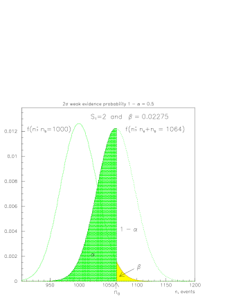
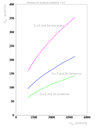
Figure 1: The case $n_{b}\gg 1$. Poisson distributions with parameters $\lambda=1000$ (left) and $\lambda=1064$ (right). Here $1-\alpha=0.5$ and $\beta=0.02275$ (i.e. $S_{1}=2$).

Figure 2: The case $n_{b}\gg 1$. Dependences $n_{s}$ versus $n_{b}$ for $S_{1}=5$, $S_{1}=3$ and $S_{1}=2$ coincide with $5\sigma$ discovery, $3\sigma$ strong evidence, and $2\sigma$ weak evidence curves, correspondingly. The probability of discovery $1-\alpha=0.5$.

The significance $S_{1}$ is determined by the formula (17) and it is often used in experiment proposals [1, 4].

For $1-\alpha>0.5$ (see Fig.3 for an illustration) the parameter $n_{0}$ in formula (14) is equal to

$$n_{0}=n_{s}+n_{b}-k(\alpha)\sqrt{n_{s}+n_{b}},$$ (18)

where $k(\alpha)$: $k(0.5)=0$; $k(0.25)=0.66$; $k(0.1)=1.28$; $k(0.05)=1.64$ (as an example, Tab.28.1 [3]). The effective significance $s$ in the equation (8) (i.e. corrected significance $S_{1}$, corresponding the discovery probability $1-\alpha$) has the form

$$s=\frac{n_{s}}{\sqrt{n_{b}}}-k({\alpha})\sqrt{1+\frac{n_{s}}{n_{b}}}$$ (19)

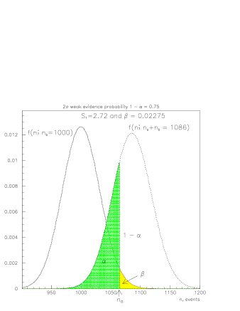
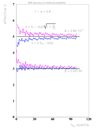
Figure 3: The case $n_{b}\gg 1$ and $S_{1}=2.72$. Poisson distributions with parameters $\lambda=1000$ (left) and $\lambda=1086$ (right). Here $1-\alpha=0.75$ and $\beta=0.02275$ (i.e. effective $s=2$).

Figure 4: The estimation of effective significance $s$ for given $\beta$ and $1-\alpha$.

So, we see that the asymptotic formula (17) for the significance $s$ is valid only for $1-\alpha=0.5$.

As it has been shown in refs. [9, 10] the more proper of the significance in planned experiments is $2\cdot S_{12}$. The generalization of this significance to the case of $1-\alpha>0.5$ looks very attractive for approximate estimation of discovery potential

$$s=2\cdot(\sqrt{n_{s}+n_{b}}-\sqrt{n_{b}})-k({\alpha}).$$ (20)

The comparison of formulae (19,20) is shown in Fig.4.

It should be stressed that very often in the conditions of planned experiment the average numbers of background and real events are not very big and we have to solve the equations (12, 13) directly to construct $5\sigma$ discovery, $3\sigma$ strong evidence and $2\sigma$ weak evidence curves. Our numerical results are presented in Figs. (5 - 10).

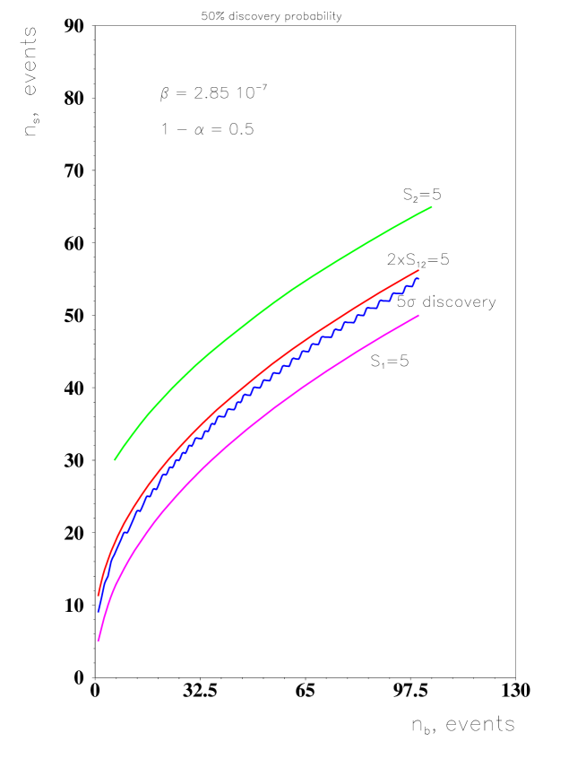
Figure 5: The $5\sigma$ discovery curve and dependences $n_{s}$ versus $n_{b}$ for $S_{1}=5$, $S_{2}=5$, $~{}2\cdot S_{12}=5$. Here $1-\alpha=0.5$ and $\beta=2.85\cdot 10^{-7}$.

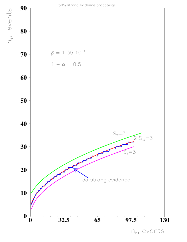
Figure 6: The $3\sigma$ strong evidence curve and dependences $n_{s}$ versus $n_{b}$ for $S_{1}=3$, $S_{2}=3$, $~{}2\cdot S_{12}=3$. Here $1-\alpha=0.5$ and $\beta=0.00135$.

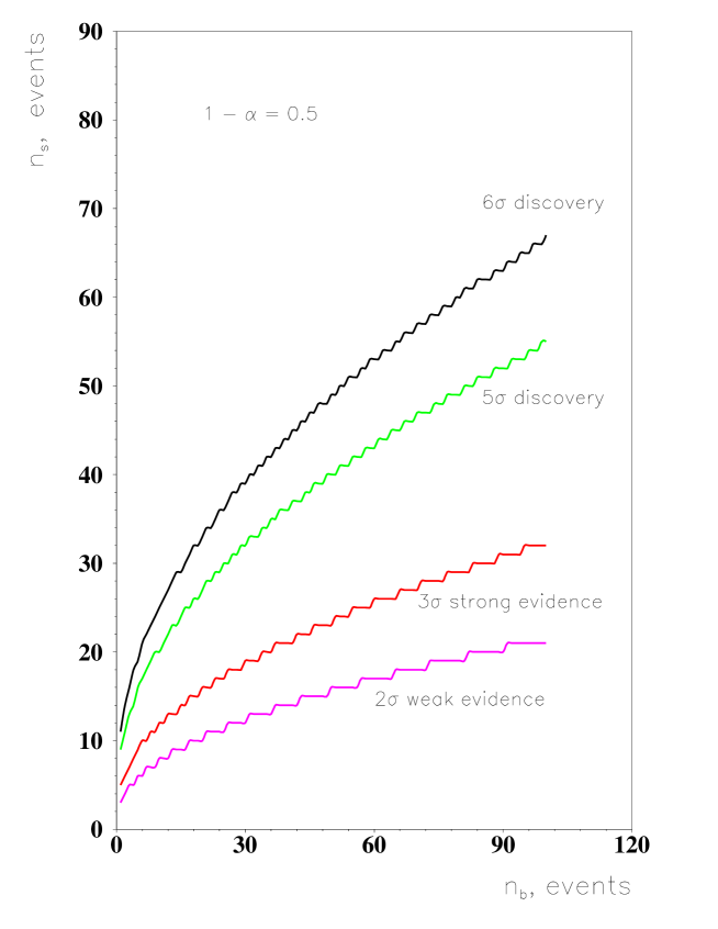
Figure 7: Dependences $n_{s}$ versus $n_{b}$ for $1-\alpha=0.5$ and for different values of $\beta$.

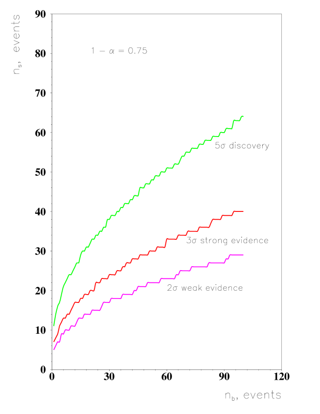
Figure 8: Dependences $n_{s}$ versus $n_{b}$ for $1-\alpha=0.75$ and for different values of $\beta$.

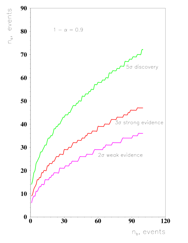
Figure 9: Dependences $n_{s}$ versus $n_{b}$ for $1-\alpha=0.9$ and for different values of $\beta$.

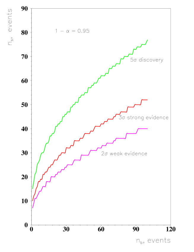
Figure 10: Dependences $n_{s}$ versus $n_{b}$ for $1-\alpha=0.95$ and for different values of $\beta$.

As an example consider the search for standard Higgs boson with a mass $m_{h}=110~{}GeV$ using the $h\rightarrow\gamma\gamma$ decay mode at the CMS detector. For total luminosity $L=3\cdot 10^{4}pb^{-1}(2\cdot 10^{4}pb^{-1})$ one can find [1] that $n_{b}=2893(1929),n_{s}=357(238)$, $\displaystyle S_{1}=\frac{n_{s}}{\sqrt{n_{b}}}=6.6(5.4)$. Using the formula (19) and Table of the standard normal probability density function [2] we find that $1-\alpha(\Delta_{dis})=0.93(0.60)$. It means that for total luminosity $L=3\cdot 10^{4}pb^{-1}(2\cdot 10^{4}pb^{-1})$ the CMS experiment will discover at $\geq 5\sigma$ level standard Higgs boson with a mass $m_{h}~{}=~{}110~{}GeV$ with a probability 93(60) percents .

For the case when we are interested in estimation of the lower bound on number $n_{s}$ of signal events (bound on new physics) we can use the equations

$$1-\alpha(\Delta)=\sum^{\infty}_{n=n_{0}(\Delta)+1}f(n;n_{b}+n_{s})$$ (21)

$$\beta(\Delta)=\sum^{\infty}_{n=n_{0}({\Delta})+1}f(n;n_{b})\geq\Delta$$ (22)

4 Exclusion limits.

It is important to know the range in which the planned experiment can exclude the presence of signal at the given confidence level ($1-\epsilon$). It means that we will have uncertainty in future hypotheses testing about non observation of signal equals to or less than $\epsilon$. In refs.[11, 12] different methods to derive exclusion limits in prospective studies have been suggested. As is seen from Fig.11 the essential differences in values of the exclusion limits take place. Let us compare these methods by the use of the equal probability test [9]. In order to estimate the various approaches of the exclusion limit determination we suppose that new physics exists, i.e. the value $n_{s}$ equals to one of the exclusion limits from Fig.11 and the value $n_{b}$ equals to the corresponding value of expected background. Then we apply the equal probability test ($f(n_{0};n_{s}+n_{b})=f(n_{0};n_{b})$) to find critical value $n_{0}$ for hypotheses testing in planned measurements (Fig.12). Here a zero hypothesis $H_{0}$ is the statement that new physics exists and an alternative hypothesis $H_{1}$ is the statement that new physics is absent. After the calculation of the Type I error $\alpha$ (the probability that the number of the observed events will be equal or less than the critical value $n_{0}$) and the Type II error $\beta$ (the probability that the number of the observed events will bigger than the critical value $n_{0}$ in the case of the absence of new physics) we can compare the methods. For this purpose the relative uncertainty [9]   $\tilde{\kappa}=\displaystyle\frac{\alpha+\beta}{2-(\alpha+\beta)}$ which will take place under hypotheses testing $H_{0}$ versus $H_{1}$ is calculated. This relative uncertainty $\tilde{\kappa}$ in case of applying the equal-probability test is a minimal relative value of the number of wrong decisions in the future hypotheses testing for Poisson distributions. It is the uncertainty in the observability of the new phenomenon. Note the $1-\tilde{\kappa}$ (the relative number of correct decisions) is a distance between two distributions (the measure of distinguishability of two Poisson processes) in frequentist sense.

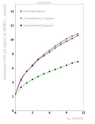
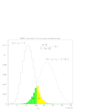
Figure 11: Estimations of the 90% CL exclusion limit on the signal in a future experiment as a function of the expected background. The method proposed in ref. [12] gives the values of exclusion limit close to ”Typical experiment” approach.

Figure 12: Equal probability test for the case $n_{b}=11$ and $n_{s}=10.61$ gives the critical value $n_{0}=16$ and, correspondingly, the relative uncertainty $\tilde{\kappa}=0.1$. It means if we observed $n_{obs}\leq n_{0}$ events in planned experiment we exclude the signal with average $n_{s}=10.61$ and above at 90%CL.

In Table 1 the result of the comparison is shown. As is seen from this Table the ”Typical experiment” approach [12] gives too small values of the exclusion limit. The difference in the 90% CL definition is the main reason of the difference between our results and the results from ref. [11]. We require that $\tilde{\kappa}$ equals to $\epsilon$, i.e. we use only one parameter ($\epsilon$) as measure of uncertainty in the hypotheses testing. In ref [11] the criterion $\beta<\Delta$ and $\displaystyle\frac{\alpha}{1-\beta}<\epsilon$ for determination of the exclusion limits has been applied. It means the experiment will observe with probability at least $1-\Delta$ at most a number of events such that the limit obtained at the $1-\epsilon$ confidence level excludes the corresponding signal. In this case two parameters ($\epsilon,~{}\Delta$) are required to construct exclusion limits. Nevertheless, we have got results close to [11] .

5 An account of systematic uncertainties related to nonexact knowledge of background and signal cross sections

In the previous sections we took into account only statistical fluctuation in the number of signal and background events and did not take into account other uncertainties. There is considered the systematic uncertainties  due to imperfect knowledge of the background and signal cross sections.

In this section we investigate the influence of the systematic uncertainties related to nonexact knowledge of the background and signal cross sections on the discovery potential in planned experiments. Denote the Born background and signal cross sections as $\sigma^{0}_{b}$ and $\sigma^{0}_{s}$. An account of one loop corrections leads to $\sigma^{0}_{b}\rightarrow\sigma^{0}_{b}(1+\delta_{1b})$ and $\sigma^{0}_{s}\rightarrow\sigma^{0}_{s}(1+\delta_{1s})$, where typically $\delta_{1b}$ and $\delta_{1s}$ are $O(0.5)$ for the LHC. Two loop corrections for most reactions at present are not known. So, we can assume that the uncertainty related with nonexact knowledge of cross sections is around $\delta_{1s}$ and $\delta_{1b}$ correspondingly. In other words we assume that exact cross sections lie in the intervals $(\sigma_{b},\sigma_{b}(1+\delta_{b}))$ and $(\sigma_{s},\sigma_{s}(1+\delta_{s}))$, where $\sigma_{b}$ and $\sigma_{s}$ are calculated at Born or one loop level of the accuracy. The average number of background and signal events lie in the intervals $(n_{b},n_{b}(1+\delta_{b}))$, $(n_{s},n_{s}(1+\delta_{s}))$, where $n_{b}=\sigma_{b}\cdot L$, $n_{s}=\sigma_{s}\cdot L$.

To determine the new physics discovery potential we again have to compare two Poisson distributions with and without new physics. Contrary to the Section 3 we have to compare the Poisson distributions in which the average numbers lie in some intervals. It means that we have to find the critical value $n_{0}$ and to estimate the influence of systematic uncertainty on the discovery probability. A priori the only thing we know is that the average number of background and signal events lie in some intervals but we do not know the exact values of the average background and signal events. Moreover we can not say anything about probability distributions of possible values $n_{b}$ and $n_{s}$ in this interval. Such distribution is absent.

An account of uncertainties related to nonexact knowledge of background and signal cross sections is straightforward and it is based on the results of Section 3. Suppose uncertainty in the calculation of exact background cross section is determined by parameter $\delta$, i.e. the exact cross section lies in the interval $(\sigma_{b},\sigma_{b}(1+\delta))$ and the exact value of average number of background events lies in the interval $(n_{b},n_{b}(1+\delta))$. Let us suppose $n_{b}\gg n_{s}$. In this instance the discovery potential most sensitive to the systematic uncertainties. Because we know nothing about possible values of average number of background events, we consider the worst case. Taking into account formulae (12) and (13) we have the formulae

$$\beta(\Delta)=\sum^{\infty}_{n=n_{0}({\Delta})+1}f(n;n_{b}(1+\delta))\leq\Delta$$ (23)

$$1-\alpha(\Delta)=\sum^{\infty}_{n=n_{0}(\Delta)+1}f(n;n_{b}+n_{s})$$ (24)

This approach allows estimate the scale of influence of background uncertainty to observability of signal. As an application of formulae (23,24) consider the case $n_{b}=n_{s}=100$ (typical case for the search for supersymmetry at LHC). For such values of $n_{s}$ and $n_{b}$ and for $\delta$= 0., 0.1, 0.25, 0.5 we find that $1-\alpha(\Delta_{dis})$ = 0.9996, 0.9924, 0.8476, 0.137, correspondingly. So, we see that the uncertainty in the calculations of background cross section is extremely essential for the determination of the LHC discovery potential. Some other examples are presented in Tables 2-7 and in Figs.13-14.

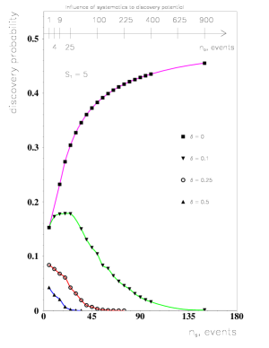
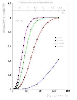
Figure 13: Discovery probability versus $n_{s}$ for different values of systematic uncertainty $\delta$ for the case $S_{1}=5$.

Figure 14: Discovery probability versus $n_{s}$ for different values of systematic uncertainty $\delta$ for the case $n_{s}=n_{b}$.

6 Conclusions

In this paper we have described a method to estimate the discovery potential and exclusion limits on new physics in planned experiments where only the average number of background $n_{b}$ and signal events $n_{s}$ is known. We have found that in this case the more proper definition of the significance (for $\alpha=0.5$) is $2\cdot S_{12}=2(\sqrt{n_{s}+n_{b}}-\sqrt{n_{b})}$ in comparison with often used expressions for the significances $S_{1}=\displaystyle\frac{n_{s}}{\sqrt{n_{b}}}$ and $S_{2}=\displaystyle\frac{n_{s}}{\sqrt{n_{s}+n_{b}}}$. For $1-\alpha>0.5$ we have additional additive contribution to the significance (see approximate formulae 19-20 of estimation of discovery potential for given discovery probability). As a result, the effective significance $s$ of signal for given probability of observation is proposed. The results of direct calculations of dependences $n_{s}$ versus $n_{b}$ for different discovery probabilities and significances are presented. We estimate the influence of systematic uncertainty related to nonexact knowledge of signal and background cross sections on the probability to discover new physics in planned experiments. An account of such kind of systematics is very essential in the search for supersymmetry and leads to an essential decrease in the probability to discover new physics in future experiments. The texts of programs can be found in http://home.cern.ch/bityukov.

We are grateful to Fred James, V.A.Matveev and V.F.Obraztsov for the interest and useful comments. S.B. thanks Bob Cousins, George Kahrimanis, James Linnemann, Louis Lyons, Tony Vaiciulis, Alex Read, Byron Roy and Pekka Sinervo for very useful discussions. S.B. would like to thank James Stirling, Mike Whalley and Linda Wilkinson for having organized this interesting Conference which is the wonderful opportunity for exchange of ideas. This work has been supported by CERN-INTAS 99-0377. The work of S.B. is also supported by CERN-INTAS 00-0440.

Table 1: The comparison of the different approaches to determination of the exclusion limits. The $\alpha$ and the $\beta$ are the Type I and the Type II errors under the equal probability test. The $\tilde{\kappa}$ equals to $\displaystyle\frac{\alpha+\beta}{2-(\alpha+\beta)}$.

		this	paper			ref.	[11]			ref.	[12]
$n_{b}$	$n_{s}$	$\alpha$	$\beta$	$\tilde{\kappa}$	$n_{s}$	$\alpha$	$\beta$	$\tilde{\kappa}$	$n_{s}$	$\alpha$	$\beta$	$\tilde{\kappa}$
1	4.31	0.10	0.08	0.10	4.45	0.09	0.08	0.09	3.30	0.20	0.08	0.16
2	5.54	0.13	0.05	0.10	5.50	0.13	0.05	0.10	3.90	0.16	0.14	0.18
3	6.32	0.10	0.08	0.10	6.40	0.09	0.08	0.10	4.40	0.14	0.18	0.19
4	7.19	0.13	0.05	0.10	7.25	0.13	0.05	0.10	4.80	0.23	0.11	0.20
5	7.71	0.11	0.07	0.10	7.90	0.10	0.07	0.09	5.20	0.20	0.13	0.20
6	8.26	0.10	0.08	0.10	8.41	0.09	0.08	0.10	5.50	0.19	0.15	0.20
7	8.83	0.08	0.10	0.10	9.00	0.08	0.10	0.10	5.90	0.17	0.17	0.20
8	9.36	0.12	0.06	0.10	9.70	0.10	0.06	0.09	6.10	0.17	0.18	0.21
9	9.76	0.11	0.07	0.10	10.16	0.09	0.07	0.09	6.40	0.16	0.20	0.22
10	10.17	0.10	0.08	0.10	10.50	0.09	0.08	0.09	6.70	0.22	0.14	0.22
11	10.61	0.08	0.11	0.10	10.80	0.08	0.09	0.10	6.90	0.21	0.15	0.22

Table 2: The dependence of $1-\alpha(\Delta_{dis})$ on $n_{s}$ and $n_{b}$ for $S_{1}=5$ and different values of $\delta$. $\Delta_{dis}=2.85\cdot 10^{-7}$.

$n_{s}$	$n_{b}$	$\delta=0.0$	$\delta=0.1$	$\delta=0.25$	$\delta=0.5$
5	1	0.1528	0.1528	0.0839	0.0426
10	4	0.2441	0.1728	0.0765	0.0288
15	9	0.2323	0.1775	0.0678	0.0206
20	16	0.2737	0.1783	0.0609	0.0071
25	25	0.3041	0.1779	0.0424	0.0020
30	36	0.3273	0.1480	0.0315	0.0005
35	49	0.3456	0.1502	0.0192	0.0001
40	64	0.3603	0.1305	0.0098
45	81	0.3725	0.1157	0.0068
50	100	0.3828	0.1042	0.0032
55	121	0.3915	0.0833	0.0015
60	144	0.3990	0.0773	0.0008
65	169	0.4055	0.0640	0.0004
70	196	0.4113	0.0538	0.0002
75	225	0.4163	0.0459	0.0001
80	256	0.4209	0.0397
85	289	0.4249	0.0310
90	324	0.4286	0.0246
95	361	0.4319	0.0197
100	400	0.4350	0.0161
150	900	0.4550	0.0011

Table 3: The dependence of $1-\alpha(\Delta_{dis})$ on $n_{s}$ and $n_{b}$ for $S_{2}\approx 5$ and different values of $\delta$.

$n_{s}$	$n_{b}$	$\delta=0.$	$\delta=0.1$	$\delta=0.25$	$\delta=0.5$
26	1	1.0000	1.0000	0.9999	0.9998
29	4	0.9992	0.9983	0.9940	0.9825
33	9	0.9909	0.9856	0.9524	0.8786
37	16	0.9725	0.9473	0.8491	0.5730
41	25	0.9418	0.8806	0.6606	0.2457
45	36	0.9016	0.7622	0.4705	0.0696
50	49	0.8774	0.7058	0.3208	0.0222
55	64	0.8546	0.6206	0.1909	0.0044
100	300	0.6803	0.1110	0.0001
150	750	0.6224	0.0084

Table 4: $n_{s}=\frac{1}{5}\cdot n_{b}$. The dependence of $1-\alpha(\Delta_{dis})$ on $n_{s}$ and $n_{b}$ for different values of $\delta$.

$n_{s}$	$n_{b}$	$\delta=0.$	$\delta=0.1$
50	250	0.0319	0.0003
100	500	0.2621	0.0023
150	750	0.6224	0.0084
200	1000	0.8671	0.0232
250	1250	0.9644	0.0513
300	1500	0.9926	0.0920
350	1750	0.9988	0.1500
400	2000	0.9998	0.2156

Table 5: $n_{s}=\frac{1}{10}\cdot n_{b}$. The dependence of $1-\alpha(\Delta_{dis})$ on $n_{s}$ and $n_{b}$.

$n_{s}$	$n_{b}$	$\delta=0.$
50	500	0.0030
100	1000	0.0327
150	1500	0.1214
200	2000	0.2781
250	2500	0.4721
300	3000	0.6514
350	3500	0.7919
400	4000	0.8878

Table 6: $n_{s}$ = $n_{b}$. The dependence of $1-\alpha(\Delta_{dis})$ on $n_{s}$ and $n_{b}$ for different values of $\delta$.

$n_{s}$	$n_{b}$	$\delta=0.$	$\delta=0.1$	$\delta=0.25$	$\delta=0.5$
2	2	0.0009	0.0003	0.0001	0.00002
4	4	0.0037	0.0016	0.0003	0.00003
6	6	0.0061	0.0030	0.0007	0.00006
8	8	0.0131	0.0075	0.0022	0.00013
10	10	0.0343	0.0135	0.0027	0.0002
12	12	0.0467	0.0206	0.0050	0.0003
14	14	0.0822	0.0283	0.0080	0.0004
16	16	0.0956	0.0512	0.0116	0.0007
18	18	0.1401	0.0609	0.0156	0.0007
20	20	0.1904	0.0925	0.0200	0.0012
24	24	0.3005	0.1402	0.0395	0.0017
28	28	0.4122	0.2280	0.0655	0.0031
32	32	0.5166	0.2821	0.0969	0.0050
36	36	0.6089	0.3773	0.1323	0.0054
40	40	0.7268	0.4703	0.1704	0.0076
50	50	0.8762	0.6688	0.2872	0.0181
60	60	0.9477	0.8309	0.4397	0.0332
70	70	0.9831	0.9067	0.5784	0.0520
80	80	0.9949	0.9575	0.6929	0.0737
100	100	0.9997	0.9938	0.8641	0.1527
150	150	1.0000	1.0000	0.9914	0.4163

Table 7: $n_{s}~{}=~{}0.5\cdot n_{b}$. The dependence of $1-\alpha(\Delta_{dis})$ on $n_{s}$ and $n_{b}$ for different values of $\delta$.

$n_{s}$	$n_{b}$	$\delta=0.$	$\delta=0.1$	$\delta=0.25$
2	4	0.0002	0.0001	0.0000
4	8	0.0003	0.0001	0.0000
6	12	0.0010	0.0002	0.0000
8	16	0.0017	0.0005	0.0000
10	20	0.0040	0.0009	0.0001
12	24	0.0071	0.0012	0.0001
14	28	0.0111	0.0023	0.0001
16	32	0.0156	0.0025	0.0002
18	36	0.0206	0.0039	0.0002
20	40	0.0341	0.0056	0.0003
24	48	0.0589	0.0099	0.0003
28	56	0.0885	0.0149	0.0005
32	64	0.1107	0.0259	0.0008
36	72	0.1796	0.0329	0.0013
40	80	0.2171	0.0482	0.0016
50	100	0.3828	0.1042	0.0032
60	120	0.5396	0.1753	0.0061
70	140	0.6947	0.2539	0.0099
80	160	0.8076	0.3578	0.0144
100	200	0.9311	0.5537	0.0319
150	300	0.9979	0.8861	0.1153

References

- [1] The Compact Muon Solenoid. Technical Proposal, CERN/LHCC 94 -38, 1994.
- [2] W.T.Eadie, D.Drijard, F.E.James, M.Roos, and B.Sadoulet, Statistical Methods in Experimental Physics, North Holland, Amsterdam, 1971. A.G.Frodesen, O.Skjeggestad, H.Tft, Probability and Statistics in Particle Physics, UNIVERSITETSFORLAGET, Bergen-Oslo-Troms, 1979.
- [3] Particle Data Group, D.E. Groom et al., Eur.Phys.J. C15 (2000) 1 (Section 28).
- [4] ATLAS Detector and Physics Performance, TDR, CERN/LHCC/99-15, p.467, CERN, May, 1999.
- [5] See as an example: D.Denegri, L.Rurua and N.Stepanov, Detection of Sleptons in CMS, Mass Reach, CMS Note CMS TN/96-059, October 1996. F.Charles, Inclusive Search for Light Gravitino with the CMS Detector, CMS Note 97/079, September 1997. S.Abdullin, Search for SUSY at LHC: Discovery and Inclusive Studies, Presented at International Europhysics Conference on High Energy Physics, Jerusalem, Israel, August 19-26, 1997, CMS Conference Report 97/019, November 1997.
- [6] N.Brown, Degenerate Higgs and Z Boson at LEP200, Z.Phys., C49, 1991, p.657. H.Baer, M.Bisset, C.Kao and X.Tata, Observability of decays of Higgs bosons from supersymmetry at hadron supercolliders, Phys.Rev., D46, 1992, p.1067.
- [7] S.I.Bityukov and N.V.Krasnikov, Towards the observation of signal over background in future experiments, Preprint INR 0945a/98, Moscow, 1998, also S.I.Bityukov and N.V.Krasnikov, New physics discovery potential in future experiments, Modern Physics Letters A13(1998)3235.
- [8] As an example: I.Narsky, Estimation of Upper Limits Using a Poisson Statistic, Nucl.Instrum.Meth. A450 (2000) 444.
- [9] S.I.Bityukov and N.V.Krasnikov, On observability of signal over background, Proceedings of Workshop on Confidence limits, YR, CERN-2000-005, 17-18 Jan., 2000, pp. 219-235 by James, F ed., Lyons, L ed., Perrin, Y ed.; S.I.Bityukov and N.V.Krasnikov, On the observability of a signal above background, Nucl.Instr.&Meth. A452 (2000) 518.
- [10] S.I.Bityukov and N.V.Krasnikov, Some problems of statistical analysis in experiment proposals, Proceedings of CHEP’01 International Conference on Computing in High Energy and Nuclear Physics, September 3-7, 2001, Beijing, P.R. China, Ed. H.S. Chen, Science Press, Beijing New York, p.134. http://www.ihep.ac.cn/chep01/
- [11] J.J.Hernandez, S.Navas and P.Rebecchi, Estimating exclusion limits in prospective studies of searches, Nucl.Instr.Meth. A 378, 1996, p.301, also J.J.Hernandez and S.Navas, JASP: a program to estimate discovery and exclusion limits in prospective studies of searches, Comp.Phys.Comm. 100, 1997 p.119.
- [12] T.Tabarelli de Fatis and A.Tonazzo, Expectation values of exclusion limits in future experiments (Comment), Nucl.Instr.Meth. A403, 1998, p.151.
- [13] R.D. Cousins and V.L. Highland, Incorporating systematic uncertainties into an upper limit, Nucl.Instr.Meth. A320 (1992) 331-335.
- [14] G.D’Agostini and M.Raso, Uncertainties due to imperfect knowledge of systematic effects: general considerations and approximate formulae. CERN-EP/2000-026, 1 February, 2000; also, hep-ex/0002056. 22 Feb. 2000.