Continuity of generalized parton distributions for the pion virtual Compton scattering

Abstract

We discuss a consistent treatment of the light-front gauge-boson and meson wave functions in the analyses of the generalized parton distributions(GPDs) and the scattering amplitudes in deeply virtual Compton scattering(DVCS) for the pion. The continuity of the GPDs at the crossover, where the longitudinal momentum fraction of the probed quark is same with the skewedness parameter, and the finiteness of the DVCS amplitude are ensured if the same light-front radial wave function as that of the meson bound state wave function is used for the gauge boson bound state arising from the pair-creation(or nonvalence) diagram. The frame-independence of our model calculation is also guaranteed by the constraint from the sum rule between the GPDs and the form factors.

PACS number(s): 13.40.Gp, 12.39.Ki, 13.60.Fz

I Introduction

Compton scattering provides a unique tool for studying hadronic structure. The Compton amplitude probes the hadrons through a coupling of two electromagnetic currents and thus can be regarded as a generalization of hadron form factors. For the Compton amplitude, when the initial photon is highly virtual but the final one is real, one arrives at the kinematics of deeply virtual Compton scattering(DVCS). According to the Quantum ChromoDynamics(QCD), the amplitudes at large momentum transfer factorize in the form of a convolution of a hard scattering amplitude which can be computed perturbatively from quark-gluon subprocesses multiplied by process-independent distribution amplitudes containing the bound-state nonperturbative dynamics for each of the interacting hadrons. Thus, the most important contribution to DVCS amplitude is given by the convolution of a hard quark propagator and a nonperturbative function describing long-distance dynamics which is known as “generalized parton distributions(GPDs)” and also known as “skewed parton distributions(SPDs)” [1, 2, 3]. The latter has been studied extensively in searching for possible new physics(see, for example, Ref. [4] and references therein).

The GPDs serve as a generalization of the ordinary (forward) parton distributions and provide much more direct and sensitive information on the light-front(LF) wave function of a target hadron than the hadron form factors. In particular, the momentum of the “probed quark” in GPDs is not integrated over, but rather kept fixed at longitudinal momentum fraction $x$, while for the form factor it is integrated out (due to the nonlocal current operator $\bar{\psi}(0)\gamma^{\mu}\psi(z)$ for the GPDs in contrast to the local vertex $\bar{\psi}(0)\gamma^{\mu}\psi(0)$ for the form factor). The form factors are then just moments of the GPDs. At the expense of being generalized amplitudes, the GPDs always involve the nonvalence contributions due to the nature of longitudinal asymmetry $\zeta=(P-P^{\prime})^{+}/P^{+}$(so called “skewedness” parameter) between initial($P$) and final($P^{\prime}$) hadron state momenta. While the kinematic region where the longitudinal momentum fraction $x$ of the probed quark is greater than the skewedness parameter $\zeta$ (i.e. $1>x>\zeta$) is called “DGLAP region”[5], the rest of the longitudinal momentum region $0<x<\zeta$ is called “ERBL region”[6]. The DGLAP and ERBL regions have also been denoted as the valence and nonvalence regions in the LF dynamics, respectively, because the parton-number-changing nonvalence Fock-state contributions cannot be avoided for $0<x<\zeta$ while only the parton-number-conserving valence Fock-state contributions are needed for $1>x>\zeta$. Thus, it has been a great challenge to calculate the nonvalence contributions to the GPDs in the framework of LF quantization.

Although many recent theoretical endeavors [7, 8, 9, 10, 11, 12] have been made in describing the GPDs in terms of LF wave functions, the task has not yet been satisfactory enough for practical calculations. In Refs. [8] and [9], the nonvalence contributions to the GPDs have been rewritten in terms of LF wave functions with different parton configurations. However, the representation given in Refs. [8] and [9] requires to find all the higher Fock-state wave functions while there has been relatively little progress in computing the basic wave functions of hadrons from first principles. In Refs. [10] and [11], the GPDs were expressed in terms of LF wave function but only within toy models such as the ’t Hooft model of $(1+1)$-dimensional QCD [10] and the scalar Wick-Cutkosky model [11], respectively. While these toy model analyses are helpful to gain some physical insight on the properties of the GPDs (especially, the time reversal invariance, the continuity at the crossover between the DGLAP and ERBL regions, and the sum rule constrained by the electromagnetic form factor), the real $(3+1)$-dimensional QCD motivates us to come up with the more realistic model for the application to the analysis of GPDs.

In an effort toward this direction, we have presented an effective treatment of handling the nonvalence contributions to the GPDs of the pion [12] using our LF constituent quark model(LFQM), which has been phenomenologically quite successful in describing the spacelike form factors for the electromagnetic and radiative decays of pseudoscalar and vector mesons [13, 14, 15] and the timelike weak form factors for exclusive semileptonic and rare decays of pseudoscalar mesons [16, 17, 18]. Our effective treatment of handling the nonvalence contributions is based on the covariant Bethe-Salpeter(BS) approach formulated in the LF quantization[16] which we call LFBS approach and has been previously applied to the exclusive semileptonic and rare decays of pseudoscalar mesons [17, 18] providing reasonable results compared to the data.

However, an artifact of discontinuity at $x=\zeta$ occured in our previous calculation of GPDs[12]. As we provided the reasoning[12], the discontinuity is caused by the different $x=\zeta$ behavior between the gauge boson vertex and the hadronic vertex if the wave function for the gauge boson vertex is taken differently from that for the hadronic vertex. The similar observation was made recently in Ref.[11] using a different model(scalar Wick-Cutkosky model). Such discontinuity at $x=\zeta$ may cause a divergence in the DVCS amplitude.

In this work, we improve our previous analysis[12] by taking the same LFBS approach for both vertices of meson and gauge boson and explicitly show that our reasoning presented in Ref.[12] is correct; i.e. the continuity of GPDs at the crossover($x=\zeta$) is ensured by this consistent treatment of vertices. We also discuss the value of GPDs at $x=\zeta$ in conjunction with the single spin asymmetry (SSA)[19, 20] and calculate the scattering amplitude contributing dominantly to the Compton scattering of the pion in the deeply virtual region. The paper is organized as follows. In Section II, we derive the GPDs as a nonperturbative formulation of the light-front dominated deeply virtual Compton scattering(DVCS) $\gamma^{*}\pi\to\gamma\pi$ of the pion and introduce the necessary kinematics following the notation employed by Radyushkin [3]. In Section III, we discuss the LFBS approach and present the consistent treatment of the gauge boson and hadron vertex functions in handling the nonvalence contributions to the GPDs. The implication of the vector meson dominance(VMD) at the gauge boson vertex in this improved analysis and the GPD value at $x=\zeta$ are also discussed. In Section IV, we show our numerical results for the GPDs of the pion that satisfy the continuity at the crossover and in turn give the finite scattering amplitude for DVCS of the pion. The frame-independence of our model is checked by the sum rule between the GPDs and the pion form factor. We also comment on the polynomiality conditions associated with the D-term contribution[21, 19] in ERBL region. Conclusions follow in Section V.

II Scattering Amplitude in DVCS

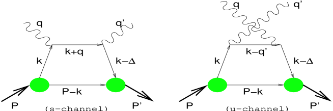
FIG. 1.: Handbag diagrams contributing dominantly to Compton scattering in the deeply virtual region. The lower soft part consists of a hadronic matrix element which is parametrized in the form of generalized parton distribution functions.

We begin with the kinematics of the virtual Compton scattering (see Fig. 1) of the pion

$$\gamma^{*}(q)+\pi(P)\to\gamma(q^{\prime})+\pi(P^{\prime}),$$ (1)

where the initial (final) hadron state is characterized by the momentum $P\;(P^{\prime})$ and the incoming spacelike virtual and outgoing real photon momenta by $q$ and $q^{\prime}$, respectively. We shall use the component notation $V=(V^{+},V^{-},{\bf V}_{\perp})$ and our metric is specified by $V^{\pm}=(V^{0}\pm V^{3})$ and $V\cdot V=V^{+}V^{-}-{\bf V}^{2}_{\perp}$.

Defining the four momentum transfer $\Delta=P-P^{\prime}$, one has $P=[P^{+},M^{2}/P^{+},0_{\perp}]$, $P^{\prime}=[(1-\zeta)P^{+},(M^{2}+\Delta^{2}_{\perp})/(1-\zeta)P^{+},-\Delta_{\perp}]$, and $\Delta=P-P^{\prime}=[\zeta P^{+},(\Delta^{2}+\Delta^{2}_{\perp})/\zeta P^{+},\Delta_{\perp}]$, where $M$ is the pion mass and $\zeta=\Delta^{+}/P^{+}$ is the skewedness parameter describing the asymmetry in plus momentum. The squared momentum transfer then reads

$$t=\Delta^{2}=2P\cdot\Delta=-\frac{\zeta^{2}M^{2}+\Delta^{2}_{\perp}}{1-\zeta}.$$ (2)

Since $\Delta^{2}_{\perp}\geq 0$, $t$ has a minimum value $-t_{\min}=\zeta^{2}M^{2}/(1-\zeta)$ at given $\zeta$. As shown in Fig. 1, the parton emitted by the pion has the momentum $k$, and the one absorbed has the momentum $k^{\prime}=k-\Delta$. As in the case of spacelike form factors, we choose a frame where the incident spacelike photon carries $q^{+}=0$: $q=[0,({\bf q}_{\perp}+\Delta_{\perp})^{2}/\zeta P^{+}+(\zeta M^{2}+\Delta^{2}_{\perp})/(1-\zeta)P^{+},{\bf q}_{\perp}$] and $q^{\prime}=[\zeta P^{+},({\bf q}_{\perp}+\Delta_{\perp})^{2}/\zeta P^{+},{\bf q}_{\perp}+\Delta_{\perp}]$.

In deeply virtual Compton scattering (DVCS) where $Q^{2}=-q^{2}$ is large compared to the mass $M$ and $-t$, one obtains $Q^{2}/(2P\cdot q)=\zeta$, i.e. $\zeta$ plays the role of the Bjorken variable in DVCS. For a fixed value of $-t$, the allowed range of $\zeta$ is given by

$$0\leq\zeta\leq\frac{(-t)}{2M^{2}}\biggl{(}\sqrt{1+\frac{4M^{2}}{(-t)}}-1\biggr{)}.$$ (3)

In the leading twist ignoring interactions at the quark-gauge boson(photon in this case) vertex, the amplitude contributing dominantly to Compton scattering in the deeply virtual region is given by

$$M^{\mu\nu}=M^{\mu\nu}_{s}+M^{\mu\nu}_{u},$$ (4)

where $M^{\mu\nu}_{s}$ and $M^{\mu\nu}_{u}$ are the $s(=(P+q)^{2})$- and $u(=(P-q^{\prime})^{2})$-channel amplitudes(see Fig. 1), respectively. The $s$-channel amplitude is given by

$$M^{\mu\nu}_{s} = -iN_{c}e^{2}_{q}\int\frac{d^{4}k}{(2\pi)^{4}}{\rm Tr}[\gamma_{5}(\not\!k+m)\gamma^{\mu}(\not\!k+\not\!q+m)\gamma^{\nu}(\not\!k-\not\!\Delta+m)\gamma_{5}(-\not\!P+\not\!k+m)]$$ (5)

$$\times \frac{H_{\rm cov}(k,P)H^{\prime}_{\rm cov}(k-\Delta,P-\Delta)}{[k^{2}-m^{2}+i\varepsilon][(k+q)^{2}-m^{2}+i\varepsilon][(k-\Delta)^{2}-m^{2}+i\varepsilon][(P-k)^{2}-m^{2}+i\varepsilon]},$$ (6)

where $N_{c}$ is the color factor and $H_{\rm cov}(k,P)[H^{\prime}_{\rm cov}(k-\Delta,P-\Delta)]$ is the covariant initial[final] state meson-quark vertex function that satisfies the BS equation. As usual in the LFBS formalism, we assume that the covariant vertex function $H_{\rm cov}(k)$ does not alter the $k^{-}$ pole structure in Eq.(5). The $u$-channel amplitude can be easily obtained by $M^{\mu\nu}_{u}=M^{\mu\nu}_{s}(q\to-q^{\prime})$.

In deeply virtual $q^{-}\simeq Q^{2}/\zeta P^{+}$ limit, one obtains $(\not\!k+\not\!q+m)\simeq\not\!q\simeq\gamma^{+}q^{-}/2$ in the trace term of Eq. (5). Consequently, combining this with the 2nd term of the denominator in Eq. (5) leads to $q^{-}/[(k+q)^{2}-m^{2}+i\varepsilon]\simeq 1/[P^{+}(x-\zeta+i\varepsilon)]$, where $x=k^{+}/P^{+}$. Similarly, one can obtain $(-q^{\prime})^{-}/[(k-q^{\prime})^{2}-m^{2}+i\varepsilon]\simeq 1/[P^{+}(x-i\varepsilon)]$ from the $u$-channel amplitude.

Adding these two $s$- and $u$-channel amplitudes, we obtain the Compton scattering amplitude in DVCS limit as follows

$$M^{IJ}=\epsilon^{I}_{\mu}\epsilon^{*J}_{\nu}M^{\mu\nu} = -\frac{iN_{c}}{2P^{+}}e^{2}_{q}\int\frac{d^{4}k}{(2\pi)^{4}}\biggl{(}\frac{1}{x-\zeta+i\varepsilon}+\frac{1}{x-i\varepsilon}\biggr{)}H_{\rm cov}(k,P)H^{\prime}_{\rm cov}(k-\Delta,P-\Delta)$$ (7)

$$\times \frac{{\rm Tr}[\gamma_{5}(\not\!k+m)\not\!\epsilon^{I}\gamma^{+}\not\!\epsilon^{*J}(\not\!k-\not\!\Delta+m)\gamma_{5}(-\not\!P+\not\!k+m)]}{[k^{2}-m^{2}+i\varepsilon][(k-\Delta)^{2}-m^{2}+i\varepsilon][(P-k)^{2}-m^{2}+i\varepsilon]}.$$ (8)

For circularly polarized($\epsilon^{+}=0$) initial and final photons($I,J$ are $\uparrow$ or $\downarrow$), we obtain from Eq. (7)

$$\not\!\epsilon^{I}\gamma^{+}\not\!\epsilon^{*J} = (\epsilon^{I}_{\perp}\cdot\epsilon^{*J}_{\perp})\gamma^{+}+i(\epsilon^{I}_{\perp}\times\epsilon^{*J}_{\perp})_{3}\gamma^{+}\gamma_{5},$$ (9)

where we use the identities $(\gamma^{+})^{2}=0$, $\gamma^{1}\gamma^{+}\gamma^{1}=\gamma^{2}\gamma^{+}\gamma^{2}=\gamma^{+}$ and $\gamma^{1}\gamma^{+}\gamma^{2}=-\gamma^{2}\gamma^{+}\gamma^{1}=i\gamma^{+}\gamma_{5}$. Equation (9) reduces to $\gamma^{+}(1\pm\gamma_{5})$ for the parallel helicities(i.e. $+$ for $\uparrow\uparrow$ and $-$ for $\downarrow\downarrow$) and zero otherwise. Since the axial current $\gamma^{+}\gamma_{5}$ does not contribute to the integral, i.e. $\sim({\bf k}_{\perp}\times\Delta_{\perp})$ after the trace calculation, we shall omit this term from now on.

Then, the DVCS amplitude(i.e. photon helicity amplitude) can be rewritten as the factorized form of hard and soft amplitude

$$M^{\uparrow\uparrow}(P,q,P^{\prime})=M^{\downarrow\downarrow}(P,q,P^{\prime}) = -e^{2}_{q}\int\;dx\biggl{(}\frac{1}{x-\zeta+i\varepsilon}+\frac{1}{x-i\varepsilon}\biggr{)}{\cal F}_{\pi}(\zeta,x,t),$$ (10)

where

$${\cal F}_{\pi}(\zeta,x,t)= = \frac{iN_{c}}{2}\int\frac{dk^{-}d^{2}{\bf k}_{\perp}}{2(2\pi)^{4}}H_{\rm cov}(k,P)H^{\prime}_{\rm cov}(k-\Delta,P-\Delta)$$ (11)

$$\times \frac{{\rm Tr}[\gamma_{5}(\not\!k+m)\gamma^{+}(\not\!k-\not\!\Delta+m)\gamma_{5}(-\not\!P+\not\!k+m)]}{[k^{2}-m^{2}+i\varepsilon][(k-\Delta)^{2}-m^{2}+i\varepsilon][(P-k)^{2}-m^{2}+i\varepsilon]}.$$ (12)

The function ${\cal F}_{\pi}(\zeta,x,t)$ is so called “generalized parton distributions” and it manifests characteristics of the ordinary(forward) quark distribution in the limit of $\zeta\to 0$ and $t\to 0$. On the other hand, the first moment of the ${\cal F}_{\pi}(\zeta,x,t)$ is related to the form factor by the following sum rules [2, 3]:

$$\int^{1}_{0}\frac{dx}{1-\frac{\zeta}{2}}{\cal F}_{\pi}(\zeta,x,t)=F_{\pi}(t).$$ (13)

In general, the polynomiality conditions for the moments of the GPDs[23, 24] defined by

$$\int^{1}_{0}\frac{dx}{1-\frac{\zeta}{2}}x^{n-1}{\cal F}_{\pi}(\zeta,x,t)=F_{n}(\zeta,t)$$ (14)

require that the highest power of $\zeta$ in the polynomial expression of $F_{n}(\zeta,t)$ should not be larger than $n$. These polynomiality conditions are fundamental properties of the GPDs which follow from the Lorentz invariance. We comment on how our model calculations satisfy the polynomiality conditions in Section IV(numerical results).

An important feature of the DVCS amplitude given by Eq. (10) is that it depends only on the skewedness parameter $\zeta=Q^{2}/(2P\cdot q)$ for large $Q^{2}$ and fixed $|t|(\leq Q^{2})$, i.e. DVCS is equivalent to an inclusive process exhibiting the Bjorken scaling $x_{Bj}=\zeta$. Note also from Eq. (10) that the imaginary part of the DVCS amplitude is proportional to ${\cal F}_{\pi}(\zeta,\zeta,t)$. The single spin asymmetry(SSA)[19, 20] that can be measured in the scattering of a longitudinally polarized probe on an unpolarized target is proportional to the imaginary part of the amplitude, i.e. the value of ${\cal F}_{\pi}(\zeta,\zeta,t)$. The recent measurements of SSA for the proton target have been reported by HERMES [25] and CLAS [26] collaborations. We discuss the value of ${\cal F}_{\pi}(\zeta,\zeta,t)$ in Section III C.

III Generalized parton distributions in light-front Bethe-Salpeter approach

The GPDs entering as nonperturbative information in DVCS as shown in Fig. 1 can be represented by Fig. 2(a) where the small white blob shown in Fig. 2(a) represents the composite(nonlocal) operator [3] at the quark-gauge boson vertex. Since the longitudinal component, $\Delta^{+}=\zeta P^{+}$, of the momentum transfer $\Delta=P-P^{\prime}$ is in general nonzero, the covariant diagram Fig. 2(a) is represented by the sum of the LF valence diagram (b) defined in $\zeta<x<1$ (DGLAP) region and the nonvalence diagram (c) defined in $0<x<\zeta$ (ERBL) region. As one can see from Fig. 2(b) and (c), the large white blobs at the meson-quark vertices in (b) and (c) represent the ordinary LF wave function. However, the large black blob in (c) cannot be represented by the ordinary LF wave function since it is no longer a bound state vertex but non-wave-function vertex. This non-wave-function vertex causes the main source of difficulty in representing the GPDs(as well as the timelike form factor) in terms of light-front wave function. However, in a covariant BS formalism it can be represented as an analytic continuation of the usual BS amplitude.

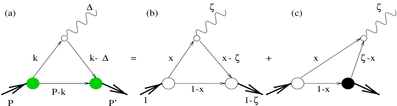
FIG. 2.: Diagrams for GPDs in different kinematic regions for the case $\zeta>0$: The covariant diagram (a) corresponds to the sum of the LF valence diagram (b) defined in DGLAP($\zeta<x<1$) region and the nonvalence diagram (c) defined in ERBL($0<x<\zeta$) region. The large white and black blobs at the meson-quark vertices in (b) and (c) represent the ordinary LF wave function and the nonvalence wave function vertices, respectively. The small white blob at the quark-gauge boson vertex indicates the nonlocality of the vertex.

In our previous work [12], we have derived the GPDs of the pion starting from the covariant BS amplitude of the current ${\cal J}$(see Eq. (12) in [12]), which is essentially the same calculation of ${\cal F}_{\pi}(\zeta,x,t)$ given by Eq. (11). Since the detailed procedures for obtaining the effective solution for the non-wave-function vertex have been given in [12], here we only briefly present the salient points of our previous effective method [12] before we discuss the new treatment of the quark-gauge boson vertex function to ensure the continuity of the GPDs at the crossover($x=\zeta$) between the DGLAP and ERBL regions.

A Brief review of our previous method [12]

The essential feature of our approach is to consider the light-front wave function as the solution of light-front Bethe-Salpeter equation(LFBSE) given by [12, 16, 27, 28]

$$(M^{2}-M^{\prime 2}_{0})\chi^{\prime}(x^{\prime}_{i},{\bf k^{\prime}}_{i\perp}) = \int^{1}_{0}[dy^{\prime}][d^{2}{\bf l^{\prime}}_{\perp}]{\cal K}(x^{\prime}_{i},{\bf k^{\prime}}_{i\perp};y^{\prime}_{j},{\bf l^{\prime}}_{j\perp})\chi^{\prime}(y^{\prime}_{j},{\bf l^{\prime}}_{j\perp}),$$ (15)

where ${\cal K}$ is the BS kernel which in principle includes all the higher Fock-state contributions, $M^{\prime 2}_{0}=(m^{2}+{\bf k^{\prime}}^{2}_{\perp})/x^{\prime}+(m^{2}+{\bf k^{\prime}}^{2}_{\perp})/(1-x^{\prime})$ is the invariant mass, and $\chi^{\prime}(x^{\prime}_{i},{\bf k^{\prime}}_{i\perp})$ is the (final state) BS amplitude with the internal momenta of the (struck) quark for the final state, $x^{\prime}=(x-\zeta)/(1-\zeta)$ and ${\bf k^{\prime}}_{\perp}={\bf k}_{\perp}+x^{\prime}\Delta_{\perp}$. The internal momenta of the (struck) quark after the kernel are given by $y^{\prime}=(y-\zeta)/(1-\zeta)$ and ${\bf l^{\prime}}_{\perp}={\bf l}_{\perp}+y^{\prime}\Delta_{\perp}$ so that the integration of $y^{\prime}$ runs from 0 to 1(or $y$ runs from $\zeta$ to 1). Note also $d^{2}{\bf l^{\prime}}_{\perp}=d^{2}{\bf l}_{\perp}$ for a given $y^{\prime}$. We define the valence BS amplitude(i.e. $x>\zeta$) as $\chi_{(2\to 2)}$ and the nonvalence BS amplitude(i.e. $x<\zeta$) as $\chi_{(1\to 3)}$ where the subscript indicates the parton number before and after the kernel. Both the valence and nonvalence BS amplitudes are solutions to Eq. (15). As illustrated in Fig. 2(c), the nonvalence BS amplitude is an analytic continuation of the valence BS amplitude. In the LFQM the relationship between the BS amplitudes in the two regions is given by [12, 16]

$$(M^{2}-M^{\prime 2}_{0})\chi^{\prime}_{(1\to 3)}(x^{\prime}_{i},{\bf k^{\prime}}_{i\perp}) = \int^{1}_{0}[dy^{\prime}][d^{2}{\bf l}_{\perp}]{\cal K}(x^{\prime}_{i},{\bf k^{\prime}}_{i\perp};y^{\prime}_{j},{\bf l^{\prime}}_{j\perp})\chi^{\prime}_{(2\to 2)}(y^{\prime}_{j},{\bf l^{\prime}}_{j\perp}),$$ (16)

where again the kernel includes in principle all the higher Fock-state contributions because all the higher Fock components of the bound-state are ultimately related to the lowest Fock component with the use of kernel as illustrated in Fig. 3.

FIG. 3.: Non-wave-function vertex(black blob) linked to an ordinary light-front wave function(white blob).

After the Cauchy integration over $k^{-}$ in Eq. (11), we obtain the valence($\zeta\leq x\leq 1$) and nonvalence($0\leq x\leq\zeta$) contributions to the GPDs of the pion as follows

$${\cal F}^{val}_{\pi}(\zeta,x,t) = \frac{N_{c}}{2x(1-x)x^{\prime}}\int\frac{d^{2}{\bf k}_{\perp}}{16\pi^{3}}\chi_{(2\to 2)}(x,{\bf k}_{\perp})S^{+}_{val}(x,{\bf k}_{\perp})\chi^{\prime}_{(2\to 2)}(x^{\prime},{\bf k}^{\prime}_{\perp}),$$ (17)

and

$${\cal F}^{nv}_{\pi}(\zeta,x,t) = \frac{-N_{c}}{2x(1-x)(1-x^{\prime\prime})}\int\frac{d^{2}{\bf k}_{\perp}}{16\pi^{3}}\chi_{(2\to 2)}(x,{\bf k}_{\perp})S^{+}_{nv}(x,{\bf k}_{\perp})\chi^{g}(x^{\prime\prime},{\bf k^{\prime\prime}}_{\perp})$$ (18)

$$\times \int^{1}_{0}\frac{dy^{\prime}}{y^{\prime}(1-y^{\prime})}\int d^{2}{\bf l}_{\perp}{\cal K}(x^{\prime},{\bf k^{\prime}}_{\perp};y^{\prime},{\bf l^{\prime}}_{\perp})\chi^{\prime}_{(2\to 2)}(y^{\prime},{\bf l^{\prime}}_{\perp}),$$ (19)

where Eq. (16) has been used for the non-wave-function vertex as shown in Fig. 3[or Fig. 2(c)]. The trace terms of the quark propagators, i.e. $S^{+}_{val}(x,{\bf k}_{\perp})$ and $S^{+}_{nv}(x,{\bf k}_{\perp})$, are given by Eqs. (21) and (25) in Ref. [12], respectively. The light-front vertex functions of the initial[final] hadron $\chi_{(2\to 2)}[\chi^{\prime}_{(2\to 2)}]$ and the gauge boson $\chi^{g}$ are given by

$$\chi_{(2\to 2)}(x,{\bf k}_{\perp}) = \frac{h_{LF}}{M^{2}-M^{2}_{0}},\;\chi^{\prime}_{(2\to 2)}(x^{\prime},{\bf k^{\prime}}_{\perp})=\frac{h^{\prime}_{LF}}{M^{2}-M^{\prime 2}_{0}},\;\chi^{g}(x^{\prime\prime},{\bf k^{\prime\prime}}_{\perp})=\frac{1}{\Delta^{2}-M^{\prime\prime 2}_{0}},$$ (20)

where $x^{\prime\prime}=x/\zeta$, ${\bf k^{\prime\prime}}_{\perp}={\bf k}_{\perp}+x^{\prime\prime}\Delta_{\perp}$, and $M^{\prime\prime 2}_{0}=({\bf k^{\prime\prime}}^{2}_{\perp}+m^{2})/x^{\prime\prime}+({\bf k^{\prime\prime}}^{2}_{\perp}+m^{2})/(1-x^{\prime\prime})$ is the invariant mass of $q\bar{q}$ pair annihilated into the gauge boson. Equations (17) and (18) were our essential results from our previous analysis [12]. Since the Eqs. (17) and (18) are divergent themselves with a constant LF vertex function $h_{LF}$, our idea is to replace the $h_{LF}$[or equivalently $\chi_{(2\to 2)}(x,{\bf k}_{\perp}$)] with the standard LF vertex function(i.e. dressed vertex) [13, 14, 16, 17, 29], which has been successful in predicting many static properties of ground state mesons. However, we left the gauge boson vertex function $\chi^{g}$ as the bare vertex given by Eq.(20) in our previous work [12]. We(as well as the authors in [11]) attributed this different treatment between gauge boson and meson vertex functions to the reason for the artifact of the discontinuity in the GPDs at the crossover($x=\zeta$) between the DGLAP and ERBL regions.

B Consistent treatment of gauge boson and meson vertex functions in LFQM: Update

As discussed in our previous work [12] and the works by others [30, 10, 11], in principle one should consider the same BS kernel ${\cal K}$ for $q{\bar{q}}$ pair annihilating into external gauge boson as that for $q\bar{q}$ pair merging into the final state meson given by Eq. (18). This is illustrated in Fig. 4 and we shall denote the GPDs coming from Figs. 4(a) and (b) as ${\cal F}^{nv}_{\pi(a)}(\zeta,x,t)$ (given by Eq. (18)) and ${\cal F}^{nv}_{\pi(b)}(\zeta,x,t)$, respectively. Adding both contributions of ${\cal F}^{nv}_{\pi(a)}$ and ${\cal F}^{nv}_{\pi(b)}$ assures the cancellation of any infrared divergence that might occur in the kernel ${\cal K}$.

FIG. 4.: Possible light-front time-ordered nonvalence diagrams with the kernel for $q\bar{q}$ pair merging into the final state meson(a) and annihilating into external gauge boson(b).

The GPDs from Figs. 4(a) and (b) can be written generically(dropping, for simplicity, relative label for internal momenta)

$$\int^{\zeta}_{0}dx{\cal F}^{nv}_{\pi(a)}(\zeta,x,t) = \int^{\zeta}_{0}dx\int d^{2}{\bf k}_{\perp}\int^{1}_{\zeta}dy\int d^{2}{\bf l}_{\perp}\chi^{\rm f}(y,{\bf l}_{\perp}){\cal K}_{a}(x,{\bf k}_{\perp};y,{\bf l}_{\perp})\chi^{g}(x,{\bf k}_{\perp})S^{+}_{nv}(x,{\bf k}_{\perp}){\tilde{\chi}}^{\rm i}_{a}(x,{\bf k}_{\perp}),$$ (21)

$$\int^{\zeta}_{0}dy{\cal F}^{nv}_{\pi(b)}(\zeta,y,t) = \int^{\zeta}_{0}dy\int d^{2}{\bf l}_{\perp}\int^{1}_{\zeta}dx\int d^{2}{\bf k}_{\perp}\chi^{\rm f}(x,{\bf k}_{\perp}){\cal K}_{b}(y,{\bf l}_{\perp};x,{\bf k}_{\perp})\chi^{g}(y,{\bf l}_{\perp})S^{+}_{nv}(x,{\bf k}_{\perp}){\tilde{\chi}}^{\rm i}_{b}(x,{\bf k}_{\perp}),$$ (22)

where the superscript i(f) in $\chi$ indicates the initial(final) valence light-front wave function(i.e. white blob in Fig. 4) and the notation of ${\tilde{\chi}}^{\rm i}_{a(b)}$ implies the product of intitial $\chi^{\rm i}_{a(b)}$ in Fig. 4a(b) and other terms(such as prefactor in Eq. (18)) that depend on the internal momentum variables. The kernel ${\cal K}_{b}(y,{\bf l}_{\perp};x,{\bf k}_{\perp})$ in Eq. (22) is equivalent to ${\cal K}_{a}(x,{\bf k}_{\perp};y,{\bf l}_{\perp})$ in Eq. (21) upon exchange of dummy variables $(x,{\bf k}_{\perp})\leftrightarrow(y,{\bf l}_{\perp})$ except an overall sign due to an exchange of quark and antiquark. If, for instance, the kernel is approximated by one boson exchange, i.e. ${\cal K}_{a}=g^{2}\theta(y-x)/(l^{+}-k^{+})[(P-k)^{-}-(l-k)^{-}-(P-l)^{-}]$ and ${\cal K}_{b}=-g^{2}\theta(x-y)/(k^{+}-l^{+})[k^{-}-l^{-}-(k-l)^{-}]$, where $y=l^{+}/P^{+}$ and $x=k^{+}/P^{+}$, then one can easily see ${\cal K}_{a}(x,y)=-{\cal K}_{b}(y\to x,x\to y)$. Note also in this simple one boson exchange case that there is only one light-front time ordered diagram in each kernel and other contributions such as $\theta(x-y)$-term in ${\cal K}_{a}$ and $\theta(y-x)$-term in ${\cal K}_{b}$ vanish since they contribute to pair creations from the vacuum. Likewise, the vertex functions $\chi^{\rm f}$ and $\chi^{g}$ in Eq. (21) are the same as those in Eq. (22) upon exchange of dummy variables $(x,{\bf k}_{\perp})\leftrightarrow(y,{\bf l}_{\perp})$.

Exchanging $(x,{\bf k}_{\perp})\leftrightarrow(y,{\bf l}_{\perp})$ in Eq. (22), we now combine these two contributions, ${\cal F}^{nv}_{\pi(a)}$ and ${\cal F}^{nv}_{\pi(b)}$, to get

$${\cal F}^{nv}_{\pi}(\zeta,x,t) = {\cal F}^{nv}_{\pi(a)}(\zeta,x,t)+{\cal F}^{nv}_{\pi(b)}(\zeta,x,t)$$ (23)

$$= \int d^{2}{\bf k}_{\perp}\int^{1}_{\zeta}dy\int d^{2}{\bf l}_{\perp}\chi^{\rm f}(y,{\bf l}_{\perp}){\cal K}(x,{\bf k}_{\perp};y,{\bf l}_{\perp})\chi^{g}(x,{\bf k}_{\perp})S^{+}_{nv}(x,{\bf k}_{\perp}){\tilde{\chi}}^{\rm i}_{a}(x,{\bf k}_{\perp})$$ (24)

$$\times \biggl{[}1-\frac{S^{+}_{nv}(y,{\bf l}_{\perp})}{S^{+}_{nv}(x,{\bf k}_{\perp})}\frac{{\tilde{\chi}}^{\rm i}_{b}(y,{\bf l}_{\perp})}{{\tilde{\chi}}^{\rm i}_{a}(x,{\bf k}_{\perp})}\biggr{]},$$ (25)

where ${\cal K}={\cal K}_{a}$ and the relative($-$) sign between the two contributions assures the removal of infrared singularity at $x=y$ and ${\bf k}_{\perp}={\bf l}_{\perp}$ (see also Ref. [10]). In Eq. (23), the $(x,{\bf k}_{\perp})$ dependence in ${\cal F}^{nv}_{\pi(b)}$ comes solely from the term ${\cal K}(x,{\bf k}_{\perp};y,{\bf l}_{\perp})\chi^{g}(x,{\bf k}_{\perp})$ (i.e. upper small loop in Fig. 4(b)), which in principle includes the sum of all possible intermediate mesons being coupled to the external current.

By putting the relative label of internal momenta back into Eq. (23), we obtain the same form of ${\cal F}^{nv}_{\pi}$ as that given by Eq. (18)

$${\cal F}^{nv}_{\pi}(\zeta,x,t) = \frac{-N_{c}}{2x(1-x)(1-x^{\prime\prime})}\int\frac{d^{2}{\bf k}_{\perp}}{16\pi^{3}}\chi_{(2\to 2)}(x,{\bf k}_{\perp})S^{+}_{nv}(x,{\bf k}_{\perp})\chi^{g}(x^{\prime\prime},{\bf k^{\prime\prime}}_{\perp})$$ (26)

$$\times \int^{1}_{0}\frac{dy^{\prime}}{y^{\prime}(1-y^{\prime})}\int d^{2}{\bf l}_{\perp}{\tilde{\cal K}}(x^{\prime},{\bf k^{\prime}}_{\perp};y^{\prime},{\bf l^{\prime}}_{\perp})\chi^{\prime}_{(2\to 2)}(y^{\prime},{\bf l^{\prime}}_{\perp}),$$ (27)

but now with

$${\tilde{\cal K}}(x^{\prime},{\bf k^{\prime}}_{\perp};y^{\prime},{\bf l^{\prime}}_{\perp}) \equiv {\cal K}(x^{\prime},{\bf k^{\prime}}_{\perp};y^{\prime},{\bf l^{\prime}}_{\perp})\biggl{[}1-\frac{S^{+}_{nv}(y,{\bf l}_{\perp}){\tilde{\chi}}^{\rm i}_{b}(y,{\bf l}_{\perp})}{S^{+}_{nv}(x,{\bf k}_{\perp}){\tilde{\chi}}^{\rm i}_{a}(x,{\bf k}_{\perp})}\biggr{]}.$$ (28)

Thus, in order to make our previous model [12] more complete, the kernel ${\cal K}(x^{\prime},{\bf k^{\prime}}_{\perp};y^{\prime},{\bf l^{\prime}}_{\perp})$ given by Eq. (18) has to be replaced by ${\tilde{\cal K}}(x^{\prime},{\bf k^{\prime}}_{\perp};y^{\prime},{\bf l^{\prime}}_{\perp})$ which is free from any infrared singularity that might occur in the kernel ${\cal K}$. Since it would be a formidable task to solve the kernel ${\tilde{\cal K}}$ directly, we follow the technique illustrated in our previous analysis[12] approximating $G_{\pi}$ defined by

$$G_{\pi} \equiv \int^{1}_{0}\frac{dy^{\prime}}{y^{\prime}(1-y^{\prime})}\int d^{2}{\bf l}_{\perp}{\tilde{\cal K}}(x^{\prime},{\bf k^{\prime}}_{\perp};y^{\prime},{\bf l^{\prime}}_{\perp})\chi_{(2\to 2)}(y^{\prime},{\bf l^{\prime}}_{\perp})$$ (29)

as a constant. As we did in our previous analysis[12], we discuss the validity of a constant $G_{\pi}$ approximation in the next section (Section IV) where our numerical analysis is presented. Although the technical aspect of our numerical analysis remains same, the replacement of kernel from $\cal K$ to $\tilde{\cal K}$ amounts to the addition of new contribution ${\cal F}^{nv}_{\pi(b)}$ and thus effectively allow us to change the gauge boson wave function $\chi^{g}(x^{\prime\prime},{\bf k^{\prime\prime}}_{\perp})$ from the simple energy denominator given by Eq. (20) to the LF vertex function identical to the meson vertex function without introducing any additional parameters .

Comparing $\chi_{(2\to 2)}$ with our light-front wave function given by Ref. [13], we identify

$$\chi_{(2\to 2)}(x,{\bf k}_{\perp})=\sqrt{\frac{8\pi^{3}}{N_{c}}}\sqrt{\frac{\partial k_{z}}{\partial x}}\frac{[x(1-x)]^{1/2}}{M_{0}}\phi(x,{\bf k}_{\perp}),$$ (30)

where the Jacobian of the variable tranformation ${\bf k}=(k_{z},{\bf k}_{\perp})\to(x,{\bf k}_{\perp})$ is obtained as $\partial k_{z}/\partial x=M_{0}/[4x(1-x)]$ and the radial wave function is given by $\phi({\bf k}^{2})=\sqrt{1/\pi^{3/2}\beta^{3}}\exp(-{\bf k}^{2}/2\beta^{2})$, which is normalized as $\int d^{3}k|\phi({\bf k}^{2})|^{2}=1$. Note that the radial wave function $\phi({\bf k}^{2})$ is essentially the same as the Brodsky-Huang-Lepage [31] LF wave function $\phi^{\rm BHL}=\exp(-M^{2}_{0}/8\beta^{2})$ up to a constant factor.

Thus, the effective gauge boson wave function $\chi^{g}(x^{\prime\prime},{\bf k^{\prime\prime}}_{\perp})$ is given by

$$\chi^{g}(x^{\prime\prime},{\bf k^{\prime\prime}}_{\perp})=\sqrt{\frac{8\pi^{3}}{N_{c}}}\sqrt{\frac{\partial k^{\prime\prime}_{z}}{\partial x^{\prime\prime}}}\frac{[x^{\prime\prime}(1-x^{\prime\prime})]^{1/2}}{M^{\prime\prime}_{0}}\phi^{g}(x^{\prime\prime},{\bf k^{\prime\prime}}_{\perp}),$$ (31)

where $\partial k^{\prime\prime}_{z}/\partial x^{\prime\prime}=M^{\prime\prime}_{0}/[4x^{\prime\prime}(1-x^{\prime\prime})]$. Here, the radial wave function $\phi^{g}(x^{\prime\prime},{\bf k^{\prime\prime}}_{\perp})$ is given by

$$\phi^{g}({\bf k^{\prime\prime}}^{2})=\sqrt{\frac{1}{\pi^{3/2}\beta^{3}}}\exp(-{\bf k^{\prime\prime}}^{2}/2\beta^{2})\exp(\Delta^{2}/8\beta^{2}),$$ (32)

where ${\bf k^{\prime\prime}}^{2}=k^{\prime\prime 2}_{z}+{\bf k^{\prime\prime}}^{2}_{\perp}$ and the virtuality $\Delta^{2}=t\neq 0$.

Substituting Eqs. (30) and (31) into Eqs. (17) and (26), we obtain the valence and nonvalence contributions to the GPDs of the pion in LFQM as follows

$${\cal F}^{val}_{\pi}(\zeta,x,t) = \int d^{2}{\bf k}_{\perp}\sqrt{\frac{\partial k^{\prime}_{z}}{\partial x^{\prime}}}\sqrt{\frac{\partial k_{z}}{\partial x}}\phi^{\prime}(x^{\prime},{\bf k^{\prime}}_{\perp})\phi(x,{\bf k}_{\perp})\frac{({\bf k}_{\perp}\cdot{\bf k^{\prime}}_{\perp}+m^{2})}{\sqrt{{\bf k}^{2}_{\perp}+m^{2}}\sqrt{{\bf k^{\prime}}^{2}_{\perp}+m^{2}}},$$ (33)

and

$${\cal F}^{nv}_{\pi}(\zeta,x,t) = -\sqrt{\frac{8\pi^{3}}{N_{c}}}\biggl{(}\frac{x^{\prime\prime}}{1-x^{\prime}}\biggr{)}\int d^{2}{\bf k}_{\perp}\sqrt{\frac{\partial k_{z}}{\partial x}}\sqrt{\frac{\partial k^{\prime\prime}_{z}}{\partial x^{\prime\prime}}}\phi(x,{\bf k}_{\perp})\phi^{g}(x^{\prime\prime},{\bf k^{\prime\prime}}_{\perp})$$ (34)

$$\times \frac{{\bf k}_{\perp}\cdot{\bf k^{\prime}}_{\perp}+m^{2}+x(1-x)x^{\prime}(M^{2}-M^{2}_{0})}{\sqrt{{\bf k}^{2}_{\perp}+m^{2}}\sqrt{{\bf k^{\prime\prime}}^{2}_{\perp}+m^{2}}}\int^{1}_{0}dy^{\prime}\int d^{2}{\bf l}_{\perp}\sqrt{\frac{{\partial l^{\prime}_{z}}}{{\partial y^{\prime}}}}\frac{{\tilde{{\cal K}}}(x^{\prime},{\bf k^{\prime}}_{\perp};y^{\prime},{\bf l^{\prime}}_{\perp})}{\sqrt{{\bf l^{\prime}}^{2}_{\perp}+m^{2}}}\phi^{\prime}(y^{\prime},{\bf l^{\prime}}_{\perp}),$$ (35)

where Eq. (33) is the same as our previous formula Eq. (28) in [12] but Eq. (34) is now different from Eq. (29) in [12] due to the modification of the gauge boson vertex function. It is worthwhile to note that the nonvalence ${\cal F}^{nv}_{\pi}$ in Eq. (34) receives not only the on-mass shell propagating contribution (i.e. the term proportional to $({\bf k}_{\perp}\cdot{\bf k^{\prime}}_{\perp}+m^{2})$) but also the instantaneous contribution(i.e. the term proportional to $x(1-x)x^{\prime}(M^{2}-M^{2}_{0})$) from the spectator quark propagator. This also contrasts to the valence ${\cal F}^{val}_{\pi}$ given by Eq. (33), which receives only on-mass shell propagating contribution. As we shall show in our numerical calculation, the instantaneous contributions from the nonvalence ${\cal F}^{nv}_{\pi}$ becomes substantial for large $\zeta>0.5$.

As discussed earlier, we shall treat the last $dy^{\prime}d^{2}{\bf l}_{\perp}$-integral term in Eq. (34) as a constant $G_{\pi}$ and check if indeed a constant $G_{\pi}$ approximation is valid by varying the value of $\zeta$ in the sum rule expressed in terms of ${\cal F}^{val}_{\pi}$ and ${\cal F}^{nv}_{\pi}$, i.e.

$$F_{\pi}(t)=\int^{1}_{0}\frac{dx}{1-\frac{\zeta}{2}}{\cal F}_{\pi}(\zeta,x,t)=\int^{1}_{\zeta}\frac{dx}{1-\frac{\zeta}{2}}{\cal F}^{val}_{\pi}(\zeta,x,t)+\int^{\zeta}_{0}\frac{dx}{1-\frac{\zeta}{2}}{\cal F}^{nv}_{\pi}(\zeta,x,t),$$ (36)

for given $-t$. Varying the value of $\zeta$ in this sum rule, Eq. (36), we can also check the frame-independence of our model as we discuss in the next section(Section IV).

C The GPD value at the crossover: ${\cal F}_{\pi}(\zeta,\zeta,t)$

Although the continuity of GPDs at $x=\zeta$ is assured in our formulation presented in the last subsection (Section III B), the value of ${\cal F}_{\pi}(\zeta,\zeta,t)$ vanishes in our model calculation as we shall see in our numerical results (Section IV). The reason why this occurs in our model calculation for the meson target is because the final state meson (depicted in Fig.2(b) and Fig.4) shares the total longitudinal momentum fraction $1-\zeta$ only between the two constituents so that, as $x-\zeta\rightarrow 0$ (i.e. the struck constituent loses its longitudinal momentum completely), the single spectator-constituent carries the total longitudinal momentum fraction $1-\zeta$ and the final state two-body wavefunction at this kinematical point ($x=\zeta$) is zero. However, the situation is entirely different for the three-body wavefunction such as in the proton target because even at $x=\zeta$ the two spectator-constituents can still share the total longitudinal momentum fraction $1-\zeta$ between themselves and the final state three-body wavefunction does not vanish at $x=\zeta$. As discussed in the literature[19, 20] and mentioned in Section II, the value of GPDs at $x=\zeta$ is directly related to the SSA that can be measured in the scattering on an unpolarized target by the lepton polarized parallel or antiparallel to its direction. The recent measurements by HERMES and CLAS collaborations showed that the SSA is indeed non-zero for the proton target and our observations based on the three-body wavefunction are not inconsistent with these experimental evidences for the non-zero GPDs of proton at $x=\zeta$.

By the same reasoning, if one includes the quark-antiquark-glue three-body state (and any other multi-constituent-states) beyond the ordinary two-body ($Q\bar{Q}$) constituents in our model calculation, then it is in principle possible to get a non-zero ${\cal F}_{\pi}(\zeta,\zeta,t)$. In the chiral-quark-soliton model[21], it is shown that ${\cal F}_{\pi}(\zeta,\zeta,t)$ is non-zero. Thus, if the experiment on the pion is possible at all, then the SSA measurement would be crucial to discreminate different models and also find how much percentage of multi-constituent-component is necessary beyond our current $Q\bar{Q}$ state for the more realistic model construction. However, it is interesting to note that our current model calculation still satisfies the polynomiality conditions (See Eq.(14)) and our result on the isosinglet GPD of the pion is qualitatively very similar to the result obtained by the chiral-quark-soliton model satisfying the soft pion theorem, as we comment in the following Section (Section IV).

IV Numerical Results

In our numerical calculations, we use the model parameters $(m,\beta)=(0.22,0.3659)$ [GeV] obtained in Ref. [13] for the linear confining potential model.

In Fig. 5, we show the comparison of the $\zeta$-dependence of $G_{\pi}$ between the two gauge boson wave functions, i.e. our new gaussian type (black data), $\phi^{g}\sim\exp[(t-M^{\prime\prime 2}_{0})/8\beta^{2}]$, and the previous [12] monopole type (white data), $\phi^{g}\sim 1/(t-M^{\prime\prime 2}_{0})$ (see Eq.(20)), for a few different momentum transfers, $-t=0$ (circle), 0.5 (square), and 1.0 (triangle) [GeV²], respectively. The invariant mass of the $q\bar{q}$ pair at the gauge boson vertex is represented as $M^{2}_{g0}=M^{\prime\prime 2}_{0}$ (see Eq. (20)) in the figure. As one can see in Fig. 5, both (black and white) $G_{\pi}$ values show approximately constant behavior for small momentum transfer $-t<1$ GeV² region. It is not surprising to see that $G_{\pi}$ becomes very large as $\zeta\to 0$, however, this does not cause a significant error in our calculation because the nonvalence contribution in the very small $\zeta$ region is highly suppressed. Also, a rather large fluctuation of black data for a rather large momentum transfer region $-t=1$ GeV² (even exhibiting a sign change near $\zeta=0.3$) is neither unexpected nor troublesome because the nonvalence contribution is significantly suppressed in this large momentum transfer region where the gaussian wave function is also exponentially reduced. In order to check the reliability (i.e. frame-independence) of our constant $G_{\pi}$ approximation, we compare the exact solution of the pion electromagnetic form factor obtained from $\zeta=0$ value with that of nonzero $\zeta$ value using our constant (average) $G_{\pi}$ approximation.

FIG. 5.: Comparison of the $\zeta$-dependence of $G_{\pi}$ between our new gaussian type(black data) and previous monopole type [12](white data) gauge boson wave functions for different momentum transfers $-t=0$ (circle), 0.5(square), and 1 (triangle) [GeV²], respectively. The invariant mass of the $q\bar{q}$ pair at the gauge boson vertex is represented as $M^{2}_{g0}=M^{\prime\prime 2}_{0}$.

FIG. 6.: The effective solution of pion form factor using a common average $G_{\pi}=G_{\rm ave.}=0.12$ value with gaussian type gauge boson wave function for $\zeta=0.3$ (thin solid line) 0.6 (long-dashed line) compared with the exact solution (thick solid line) as well as experimental data [32, 33]. The dotted line represents the nonvalence contributions to the form factor for $\zeta=0.6$ case.

In Fig. 6, we show our effective solutions of the pion form factor with gaussian $\phi^{g}(x^{\prime\prime},{\bf k^{\prime\prime}}_{\perp})$ for $\zeta=0.3$ (thin solid line) and 0.6 (long-dashed line) cases obtained from our average value of $G_{\pi}=G_{\rm ave.}=0.12$ and compare them with the exact solution (thick solid line) as well as the experimental data [32, 33]. The dotted line represents the nonvalence contributions to the form factor for $\zeta=0.6$ case, which increase (decrease) as $\zeta$ gets larger (smaller). Also, there are $-t_{\rm min}$ values for nonzero $\zeta$ due to $\Delta^{2}_{\perp}\geq 0$ (see Eq. (2)). We thus use the analytic continuation by changing $\Delta_{\perp}$ to $i\Delta_{\perp}$ in Eqs. (33) and (34) to obtain the result for $0\leq-t\leq-t_{\rm min}$ where there is no singularity. A continuous behavior of the form factor near $-t_{\rm min}$ confirms the analyticity of our model calculation. As far as the $G_{\pi}$ and the form factor calculations are concerned, the results obtained from the gaussian type gauge boson wave function are overall not much different from our previous results [12] obtained from the monopole type gauge boson wave function. However, as we shall see below, they are distinguished by the calculation of the GPDs.

FIG. 7.: Generalized parton distributions of the pion at $-t=0.5$ GeV² with $\zeta=0.3$ in (a), and 0.6 in (b), respectively.

In Fig. 7, we compare the nonvalence contributions(in ERBL region) to the GPDs ${\cal F}_{\pi}(\zeta,x,t)/(1-\zeta/2)$ of the pion obtained from the gaussian type gauge boson wave function(thin solid line) with those obtained from the monopole type wave function(long-dashed line) for fixed momentum transfer $-t=0.5$ GeV² but with different skewedness parameters $\zeta=0.3$ in (a) and 0.6 in (b), respectively. The thick solid line represents the valence contribution(in DGLAP region), which is common for both gaussian and monopole type gauge boson wave functions. Our results are obtained from average values of $G_{\pi}$, i.e. $G_{\pi}=0.12$ for the gaussian type gauge boson wave function and 0.32 [12] for the monopole type gauge boson wave function. We also plot the instantaneous contributions to the GPDs with the gaussian type(dotted line) and the monopole type(dot-dashed line) gauge boson wave functions for $\zeta=0.6$ case. We note that the results of the GPDs shown in Fig. 7 with the average $G_{\pi}$ values for both gaussian and monopole type gauge boson wave function cases are very close to the exact ones, i.e. frame-independent, as one can deduce from Fig. 6 for the gaussian wave function and Fig. 9 in [12] for the monopole type wave function, respectively.

As shown in Fig. 7, the most dramatic change in our updated result of the pion GPDs is that the solutions with the gaussian type gauge boson wave function show the continuity at the crossover($x=\zeta$), while the solutions with the monopole type[12] gauge boson wave function show discontinuity at the crossover. As we discussed before, such discontinuity at $x=\zeta$ with the monopole type gauge boson wave function is just an artifact due to the different $x\rightarrow\zeta$ behavior between the gauge boson vertex ($\chi^{g}$) and the hadronic vertex ($\chi_{(2\to 2)})$ functions (see Eq.(20)). This discontinuity problem of the GPDs appeared in our previous analysis [12] is now resolved by realizing that the same type of bound state wave function should be used for both hadron and gauge boson. Furthermore, we can obtain finite results for the scattering amplitudes for the DVCS region given by Eq. (10) since both valence and nonvalence solutions of the GPDs are not only continuous but also vanish at the crossover($x=\zeta$) as well as at $x=0$. As we discussed in Section III C, ${\cal F}_{\pi}(\zeta,\zeta,t)$ can be in principle non-zero if the multi-constituent-states are included beyond the ordinary $Q\bar{Q}$ state. Within our current $Q\bar{Q}$ model, however, we have checked the $n$th moment $F_{n}(\zeta,t)$ in Eq.(14) for up to $n=3$ as well as the isosinglet GPDs. With our updated formulation presented in Section III B, we did not find any difference from our previous results, Figs. 10 and 11 of Ref.[12], based on the formulation summarized in Section III A except the change of $G_{\pi}$ value discussed above. Thus, we do not show those figures in duplication but have confirmed that the polynomiality conditions are satisfied in our current model and our result on the isosinglet GPD of the pion is qualitatively very similar to the result (Fig.5 of Ref.[21]) obtained by the chiral-quark-soliton model including the D-term in the ERBL region. The D-term generates the highest power in the polynomial, e.g. the second moment of the pion isosinglet GPD is given by $F_{2}^{I=0}(\zeta,t=0)=\frac{1}{2}(1+C\zeta^{2})$, where $C=-1/4$ in the chiral limit[21] Our model calculation from Figs. 10 and 11 of Ref.[12] gives $C=-0.2843$. Incidentally, we note from Fig.5 of Ref.[21] that the chiral-quark-soliton model not neglecting the dynamical quark mass generated in the spontaneous breaking of chiral symmetry also gives the value of $|C|$ slightly greater than 1/4.

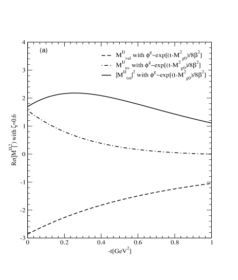
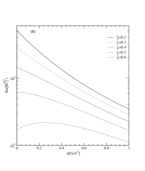
FIG. 8.: (a) The real part of the DVCS amplitude $M^{IJ}=M^{\uparrow\uparrow}+M^{\downarrow\downarrow}$(see Eq. (10)) obtained from the gaussian type gauge boson wave function and the average $G_{\pi}=0.12$ for fixed $\zeta=0.6$: The thick solid, dashed, dot-dashed lines represent the total squared amplitude Re$(M^{IJ})^{2}$, valence part of $M^{IJ}=M^{IJ}_{val}$, and nonvalence part of $M^{IJ}=M^{IJ}_{nv}$, respectively. (b) The $\zeta$ dependence of the DVCS squared amplitude Re($|M^{IJ}|^{2}$).

In Fig. 8(a), we show the real part of the DVCS squared amplitude (thick solid line), Re($|M^{IJ}|^{2}$)=Re($|M^{\uparrow\uparrow}+M^{\downarrow\downarrow}|^{2}$) =4Re($|M^{\uparrow\uparrow}|^{2}$) in Eq. (10), obtained from the gaussian type gauge boson wave function and the average $G_{\pi}=0.12$ for the range of $0\leq-t\leq 1$ [GeV²] with fixed $\zeta=0.6$. The thick dashed and dot-dashed lines represent the valence ($M^{IJ}=M^{IJ}_{val}$) and nonvalence ($M^{IJ}=M^{IJ}_{nv}$) contributions to the total amplitude, respectively. It is interesting to note that the valence and nonvalence amplitudes interfere with each other destructively not constructively. We also note that the DVCS squared amplitude Re($|M^{IJ}|^{2}$) for the monopole type gauge boson wave function shows the logarithmic divergent behavior as expected due to the discontinuity at the crossover $x=\zeta$. We thus do not present the corresponding result for the monopole type gauge boson wave function. In Fig. 8(b), we show the $\zeta$ dependence of Re($|M^{IJ}|^{2}$) for the gaussian type gauge boson wave function. In our model calculations, the DVCS squared amplitude increases as $\zeta$ decreases. As in the case of Fig. 6, we confirm the analyticity of our calculation from the continuous behavior of our results near $-t=-t_{\rm min}$.

V Conclusion

In this work, we reinvestigated our previous light-front quark model analysis [12] of the GPDs in the deeply virtual Compoton scattering (DVCS) of the pion, $\gamma^{*}\pi\to\gamma\pi$. We improved our previous effective treatment [12] of handling nonvalence (or higher Fock-states) contributions to the GPDs with the inclusion of the BS kernel for the $q\bar{q}$ pair annihilating into the gauge boson(see also [30, 10, 11] for a similar discussion) in addition to that for the $q\bar{q}$ pair merging into the final state meson(see Fig.4). It leads us to have a vector meson dominance picture at the gauge boson vertex within our constant approximation of $G_{\pi}$ in Eq. (29) and in turn to use the same type of gaussian wave function at both gauge boson and meson vertices. The continuity of the GPDs at the crossover($x=\zeta$) between the DGLAP and ERBL regions is ensured by a consistent treatment of the gauge boson and meson wave functions. Subsequently, the real part of the DVCS amplitude $M^{IJ}$ is calculated and its finiteness is confirmed (see Figs.8(a) and (b)). In our current $Q\bar{Q}$ constituent model, we obtain ${\cal F}_{\pi}(\zeta,\zeta,t)=0$ indicating that the single spectator cannot share its longitudinal momentum at $x=\zeta$. In principle, ${\cal F}_{\pi}(\zeta,\zeta,t)$ can be non-zero if our model is extended to include the multi-constituent-components. However, our current model is capable of satisfying the polynomiality conditions and yields qualitatively very similar results on the isosinglet GPD of the pion indicating that the D-term is effectively included in the ERBL region. Also, one should note that our model is not inconsistent with the recent HERMES and CLAS data on the SSA for the proton target.

Finally, the GPD of the pion is invariant under the time reversal symmetry($\Delta\to-\Delta$). As illustrated schematically in Fig. 9, it is not difficult to see that our effective method does not violate the time reversal symmetry.

FIG. 9.: Illustration of time reversal($\Delta\to-\Delta$) process of the GPDs in Fig. 4.

Using our model calculation of the DVCS amplitude in which the final photon is emitted by the pion, one can calculate the differential cross section of the virtual Compton scattering of the pion, i.e. $\pi e\to\pi e\gamma$, by incorporating the Bethe-Heitler(BH) process [34, 35] in which the final photon is emitted by either the incoming electron or the outgoing electron. Considerations along this line are in progress.

Acknowledgements

The work of HMC and LSK was supported in part by the NSF grant PHY-00070888 and that of CRJ by the US DOE under grant No. DE-FG02-96ER40947. The North Carolina Supercomputing Center and the National Energy Research Scientific Computer Center are also acknowledged for the grant of Cray time.

REFERENCES

• [1] D. M$\ddot{u}$ller, D. Robaschik, B. Geyer, F. M. Dittes, J. Ho$\check{r}$ej$\check{s}$i, Fortsch. Phys. 42, 101 (1994) [hep-ph/9812448].
• [2] X. Ji, Phys. Rev. Lett. 78, 610 (1997); Phys. Rev. D 55, 7114 (1997).
• [3] A. V. Radyushkin, Phys. Rev. D 56, 5524 (1997).
• [4] K. Goeke, M.V. Polyakov, and M. Vanderhaeghen, Prog. Part. Nucl. Phys. 47, 401 (2001).
• [5] V.N. Gribov and L.N. Lipatov, Sov. J. Phys. 15, 438 (1972); Yu.L. Dokshitzer, Sov. Phys. JETP 46, 641 (1977); G. Altarelli and G. Parisi, Nucl. Phys. B 126, 298 (1977).
• [6] A.V. Efremov and A.V. Radyushkin, Phys. Lett. B 94, 245 (1980); Theor. Math. Phys. 42, 97 (1980); S.J. Brodsky and G.P. Lepage, Phys. Lett. B 87, 359 (1979); G.P. Lepage and S.J. Brodsky, Phys. Rev. D 22, 2157 (1980).
• [7] M. Diehl, Th. Feldmann, R. Jakob, and P. Kroll, Eur. Phys. J. C, 409 (1999); Nucl. Phys. B 596, 33 (2001).
• [8] M. Diehl, Th. Feldmann, R. Jakob, and P. Kroll, Nucl. Phys. B 596, 33 (2001).
• [9] S.-J. Brodsky, M. Diehl, and D. S. Hwang, Nucl. Phys. B 596, 99 (2001).
• [10] M. Burkardt, Phys. Rev. D 62, 094003 (2000).
• [11] B. C. Tiburzi and G. A. Miller, Phys. Rev. D 65, 074009 (2002);hep-ph/0205109.
• [12] H. -M. Choi, C. -R. Ji, and L. S. Kisslinger, Phys. Rev. D 64, 093006 (2001).
• [13] H. -M. Choi and C. -R. Ji, Phys. Rev. D 59, 074015 (1999).
• [14] H. -M. Choi and C. -R. Ji, Phys. Rev. D 56, 6010 (1997).
• [15] L. S. Kisslinger, H.-M. Choi, and C.-R. Ji, Phys. Rev. D 63, 113005 (2001).
• [16] C.-R. Ji and H.-M. Choi, Phys. Lett. B 513, 330 (2001); eConf C010430: T23(2001)[hep-ph/0105248].
• [17] H. -M. Choi and C. -R. Ji, Phys. Lett. B 460, 461 (1999); Phys. Rev. D 59, 034001 (1998).
• [18] H. -M. Choi and C. -R. Ji, and L. S. Kisslinger, Phys. Rev. D 65, 074032 (2002).
• [19] N.Kivel, M.V.Polyakov and M.Vanderhaeghen, Phys. Rev. D 63, 114014 (2001).
• [20] A.Freund and M.McDermott, hep-ph/0111472.
• [21] M.V.Polyakov and C.Weiss, Phys. Rev. D 60, 114017 (1999).
• [22] A. V. Radyushkin, Phys. Rev. D 58, 114008 (1998).
• [23] X. Ji, W. Melnitchouk, and X. Song, Phys. Rev. D 56, 5511 (1997).
• [24] A. V. Radyushkin, Phys. Lett. B 449, 81 (1999).
• [25] A. Airapetian et al., Phys. Rev. Lett. 87, 182001 (2001).
• [26] S. Stepanyan et al., Phys. Rev. Lett. 87, 182002 (2001).
• [27] S. J. Brodsky, C.-R. Ji and M. Sawicki, Phys. Rev. D 32, 1530 (1985).
• [28] J. H. O. Sales, T. Frederico, B. V. Carlson, and P. U. Sauer, Phys. Rev. C 61, 044003 (2000).
• [29] W. Jaus, Phys. Rev. D 44, 2851 (1991).
• [30] M. B. Einhorn, Phys. Rev. D 14, 3451 (1976).
• [31] S. J. Brodsky, T. Huang, and G. P. Lepage, in Quarks and Nuclear Forces, edited by D. Fries and B. Zeitnitz, Springer Tracts in Modern Physics, Vol. 100 (Springer-Verlag, New York, 1982).
• [32] R. A. Amendolia et al., Phys. Lett. B 178, 435 (1985).
• [33] J. Volmer et al., Phys. Rev. Lett. 86, 1713 (2001).
• [34] M. Diehl, T. Gousset, B. Pire and J. P. Ralston, Phys. Lett. B 411, 193 (1997).
• [35] C. Unkmeir et al. Phys. Rev. C 65, 015206 (2002).