Transient domain walls and lepton asymmetry in the Left-Right symmetric model

Abstract

It is shown that the dynamics of domain walls in Left-Right symmetric models, separating respective regions of unbroken $SU(2)_{L}$ and $SU(2)_{R}$ in the early universe, can give rise to baryogenesis via leptogenesis. Neutrinos have a spatially varying complex mass matrix due to CP-violating scalar condensates in the domain wall. The motion of the wall through the plasma generates a flux of lepton number across the wall which is converted to a lepton asymmetry by helicity-flipping scatterings. Subsequent processing of the lepton excess by sphalerons results in the observed baryon asymmetry, for a range of parameters in Left-Right symmetric models.

I Introduction

Explaining the observed baryon asymmetry of the Universe within the framework of gauge theories and the standard Big Bang cosmology remains an open problem. The study has resulted in a deeper understanding of nonperturbative phenomena at finite temperature in gauge theories including supersymmetric theories. Many of the particle physics models and scenarios considered so far seem to require unnatural extensions or very special choices of parameters for successful baryogenesis; prime among these are the standard model (SM) and its minimal supersymmetric extension (MSSM), using a first order phase transition shap ; CKN ; others . Among the alternative proposals are those which rely on the presence of topological defects, viz., domain walls mencoo , and cosmic strings sbdanduay1 ; branden1 . The latter are generic to many gauge theories. What makes them especially suited for baryogenesis is their nonthermal nature soon after their formation. Unlike the need for a first order phase transition which sets severe limitations on the couplings and particle content of the model, existence of defects relies only on topological features of the vacuum manifolds and permits nonthermal effects without fine tuning.

Many special features arise when studying cosmological consequences of topological defects in any given gauge model. The Left-Right symmetric (L-R) model was studied in the context of conventional baryogenesis mechanisms in mohzha ; Frere:1992bd and in the context of domain wall mediated mechanism in lewrio . A detailed study of the possible defects existing in the L-R model was made in ywmmc . It was argued that the domain wall configurations implied by the symmetry breaking pattern present possibilities for baryogenesis. In this paper we study the interaction of neutrinos which derive Majorana masses from the scalar condensate which constitutes the domain wall. Many of the broad features encountered, e.g., asymmetric reflection and transmission of fermions from moving domain walls, have appeared in the study of electroweak baryogenesis. In the diffusion-enhanced scenario CKN driven by thick walls, the asymmetry diffusing in front of the wall is equlibrated by high temperature sphalerons. In our mechanism this is replaced by helicity flipping interactions in front of the wall which arise from the scalar condensate imparting a Majorana mass to the fermions. Our parametric answer for the unprocessed Lepton asymmetry produced in this mechanism is therefore dominated by the Majorana mass parameter $f$ in eq. (42). The scalar condensate is absent behind the wall and therefore the asymmetry that has streamed through persists.

At the completion of the $L-R$ symmetry breaking transition, a particular hypercharge ${\tilde{Y}}=I^{3}_{R}-\frac{1}{2}(B-L)$ is demonstrated to be spontaneously generated in the form of left-handed neutrinos. Due to the high-temperature electroweak sphalerons, which set $B+L=0$, this will be converted into an asymmetry of baryon minus lepton number ($B-L$). The baryon asymmetry thus generated arises in addition to that from the well-known leptogenesis fukyan ; luty mechanism due to Majorana neutrinos. However, the two mechanisms constrain the Left-Right model rather differently. The usual mechanism requires the $Z_{R}$ mass to be larger than the heavy neutrino mass luty ; plum ; buchplum . The present mechanism constrains the parameters of the Higgs sector for adequate $CP$ violation, and the Majorana Yukawa couplings as already pointed out. Our main result is the identification of broad ranges of these parameters that ensure sufficient lepton asymmetry. Further, the subsequent evolution of this asymmetry must successfully produce the abserved baryon asymmetry. This requirement can be used to constrain the temperature scale of the $L-R$ phase transition, eq. (49), or alternatively, the light neutrino mass, eq. (51).

In Harvey:1990qw and Fischler:1990gn the possibility of $B-L$ generated by any mechanism being neutralised due to presence of heavy majorana neutrino was considered. The bound first obtained in Harvey:1990qw is $20M_{\scriptscriptstyle N}\ \mbox{\raisebox{-2.58334pt}{~{}$\stackrel{{\scriptstyle>}}{{\sim}}$~{}}}\ \sqrt{T_{B-L}M_{Pl}}$ with $M_{\scriptscriptstyle N}$ the mass scale of the heavy majorana neutrino and $T_{B-L}$ the temperature at which $B-L$ originates. This is derived from lepton number depletion due to heavy neutrino mediated scattering processes and assumes $T_{B-L}>M_{\scriptscriptstyle N}$. It was argued in Fischler:1990gn that the requirement that the heavy neutrino decays occur only in out of equilibrium conditions places a more stringent bound. Using the see-saw relation, it requires

$$m_{\nu}\mbox{\raisebox{-2.58334pt}{~{}$\stackrel{{\scriptstyle<}}{{\sim}}$~{}}}m_{*}\equiv 4\pi g_{*}^{1/2}{G_{N}^{1/2}\over\sqrt{2}G_{F}}\sim 10^{-3}eV.$$ (1)

where $G_{N}$ is the Newton constant and $G_{F}$ is the Fermi constant. Current neutrino data easily suggest a larger neutrino mass. In this case it is argued that Fischler:1990gn one needs

$$T_{B-L}\mbox{\raisebox{-2.58334pt}{~{}$\stackrel{{\scriptstyle<}}{{\sim}}$~{}}}M_{\scriptscriptstyle N}={h^{2}\over 2}\left(m_{*}\over m_{\nu}\right)^{2}10^{17}GeV$$ (2)

These considerations generically need a low scale for $B-L$ creation. Detailed investigationsBuchmuller:2000as of Leptogenesis scenrios, including lepton generation mixing, show that in several specific unified models this can be achieved in the context of conventional Leptogenesis. The present mechanism has the potential of meeting the requirement of low scale $B-L$ generation in a natural way, although detailed investigations remain to be carried out. We shall return to this point in sec. VI.

The paper is organised as follows. Section II introduces the main features of the Left-Right symmetric model, synthesizing the conventions used by previous authors with the ones we follow. Section III discusses the microscopic mechanism of lepton number violation in scattering near the domain wall. It outlines the method that can be used for detailed study of lepton number creation in this context. Section IV demonstrates the existence of the conditions required for lepton number creation, in particular the CP-violating nature of the wall profiles. Section V presents a simplified version of the full theory to be studied and numerical results justifying the general conclusions of the previous section. Section VI discusses the implications to cosmology. Overall conclusions are presented in the last section.

II The Left-Right symmetric model

For the purpose of model building, Left-Right symmetry is a broad category, with several possible implementations. In this paper we shall adopt its more popular version which is desribed below. From the point of view of our mechanism, the discrete symmetry under exchange of the $SU(2)_{R}$ field content of the model with $SU(2)_{L}$ field content is crucial. The breakdown of this symmetry gives rise to domain walls whose field configuration we study in detail. The most elegant version of the model consists of identical values of the two $SU(2)$ gauge couplings in addition to a strict equality of certain scalar couplings in the Higgs potential. This may seem like an artificial requirement, considering that the two semisimple groups are independent, and there are no dynamical hints why they must be exactly same to begin with. More importantly, if this requirement is imposed an unpleasant feature arises in the context of cosmology. Breakdown of an exact discrete symmetry gives rise to stable domain walls and unless some mechanism removes them, they quickly come to dominate the energy density of the Universe, contrary to observations. Thus departure from exact symmetry is in any case a phenomenologically desirable feature. Happily, the mechanism being proposed here works well so long as the departure from exact symmetry is small so that domain walls indeed form as transient constructs. A quantitiative discussion of this is taken up in sec. IV.1.

We now recapitulate the minimal $SU(2)_{L}\otimes SU(2)_{R}\otimes U(1)_{B-L}$ model Senjanovic2 ; mohapbook . Parity is restored above an energy scale $v_{R}$, taken to be much higher than the electroweak scale, by introducing the $SU(2)_{R}$ gauge symmetry which breaks at $v_{R}$. Accordingly, a right-handed heavy neutrino species is added to each generation, and the gauge bosons consist of two triplets $W_{L}^{\mu}\equiv(3,1,0)$, $W_{R}^{\mu}\equiv(1,3,0)$ and a singlet $B^{\mu}\equiv(1,1,0)$. A Left-Right symmetric assignment of gauge SU(2) charges to the fermions shows that the new hypercharge needed to obtain the usual electric charge correctly is exactly $B-L$. It is appealing that in this model the weak hypercharge is related to known conserved charges.

The electric charge formula now assumes a Left-Right symmetric form

$$Q=T^{3}_{L}+T^{3}_{R}+\frac{B-L}{2}~{}~{},$$ (3)

where $T^{3}_{L}$ and $T^{3}_{R}$ are the weak isospin represented by $\tau^{3}/2$, and $\tau^{3}$ is the Pauli matrix.

The Higgs sector of the model is dictated by two considerations: the pattern of symmetry breaking and the small masses of the known neutrinos via the seesaw mechanism. The minimal set to achieve these goals is

$$\phi=\pmatrix{\phi_{1}^{0}&\phi_{1}^{+}\cr\phi_{2}^{-}&\phi_{2}^{0}}\equiv\pmatrix{\frac{1}{2},\frac{1}{2},0}~{}~{},$$

$$\Delta_{\scriptscriptstyle L}=\pmatrix{\frac{\delta_{\scriptscriptstyle L}^{+}}{\sqrt{2}}&\delta_{\scriptscriptstyle L}^{\scriptscriptstyle++}\cr\delta_{\scriptscriptstyle L}^{0}&-\frac{\delta_{\scriptscriptstyle L}^{+}}{\sqrt{2}}}\equiv(1,0,2)~{}~{},$$

$$\Delta_{\scriptscriptstyle R}=\pmatrix{\frac{\delta_{\scriptscriptstyle R}^{+}}{\sqrt{2}}&\delta_{\scriptscriptstyle R}^{\scriptscriptstyle++}\cr\delta_{\scriptscriptstyle R}^{0}&-\frac{\delta_{\scriptscriptstyle R}^{+}}{\sqrt{2}}}\equiv(0,1,2)~{}~{}.$$ (4)

where the electric charge assignment of the component fields has been displayed and the representation with respect to the gauge group is given in standard notation.

The minimal form of the Higgs potential needed to fulfill the main phenomenological requirements can be found in mohapbook . This is however not the most general form. In dgko as well as barenber the possibility of spontaneous CP violation was considered. In this case the couplings are chosen to be real, yet the translation invariant minimum of the potential occurs for complex VEV’s (vacuum expectation values). The absence of explicit CP-violating couplings makes it easier to accommodate phenomenological constraints on CP violation. In the cosmological context in which we treat this theory, this motivation is not as compelling. Nevertheless, the same simplifying assumption will be made here.

Consider the potential parameterized as

$$V=V_{\Phi}+V_{\Delta}+V_{\Phi\Delta}~{}~{},$$ (5)

with

$$V_{\Phi}= - \mu_{1}^{2}\rm Tr\phi\phi^{\dagger}-\mu_{2}^{2}(\rm Tr\tilde{\phi}\phi^{\dagger}+\rm Tr\phi\tilde{\phi}^{\dagger})$$ (6)

$$+ \lambda_{1}(\rm Tr\phi\phi^{\dagger})^{2}+\lambda_{2}\{(\rm Tr\tilde{\phi}\phi^{\dagger})^{2}+(\rm Tr\tilde{\phi}^{\dagger}\phi)^{2}\}$$

$$+ \lambda_{3}(\rm Tr\tilde{\phi}\phi^{\dagger})(\rm Tr\tilde{\phi}^{\dagger}\phi)+\lambda_{4}\{\rm Tr\phi^{\dagger}\phi(\rm Tr\phi^{\dagger}\tilde{\phi}+\rm Tr\tilde{\phi}^{\dagger}\phi)\}~{}~{},$$

$$V_{\Delta}= - \mu_{3}^{2}\rm Tr\Big{(}\Delta_{\scriptscriptstyle L}^{\dagger}\Delta_{\scriptscriptstyle L}+\Delta_{\scriptscriptstyle R}^{\dagger}\Delta_{\scriptscriptstyle R}\Big{)}+\rho_{1}\Big{[}\Big{(}\rm Tr(\Delta_{\scriptscriptstyle L}^{\dagger}\Delta_{\scriptscriptstyle L})\Big{)}^{2}+\Big{(}\rm Tr(\Delta_{\scriptscriptstyle R}^{\dagger}\Delta_{\scriptscriptstyle R})\Big{)}^{2}\Big{]}$$ (7)

$$+ \rho_{2}\Big{[}\rm Tr\Delta_{\scriptscriptstyle L}^{\dagger}\Delta_{\scriptscriptstyle L}^{\dagger}\rm Tr\Delta_{\scriptscriptstyle L}\Delta_{\scriptscriptstyle L}+\rm Tr\Delta_{\scriptscriptstyle R}^{\dagger}\Delta_{\scriptscriptstyle R}^{\dagger}\rm Tr\Delta_{\scriptscriptstyle R}\Delta_{\scriptscriptstyle R}\Big{]}+\rho_{3}\Big{[}\rm Tr\Big{(}\Delta_{\scriptscriptstyle L}^{\dagger}\Delta_{\scriptscriptstyle L}\Big{)}\rm Tr\Big{(}\Delta_{\scriptscriptstyle R}^{\dagger}\Delta_{\scriptscriptstyle R}\Big{)}\Big{]}$$

$$+ \rho_{4}\Big{[}\rm Tr\Delta_{\scriptscriptstyle L}\Delta_{\scriptscriptstyle L}\rm Tr\Delta_{\scriptscriptstyle R}^{\dagger}\Delta_{\scriptscriptstyle R}^{\dagger}+\rm Tr\Delta_{\scriptscriptstyle L}^{\dagger}\Delta_{\scriptscriptstyle L}^{\dagger}\rm Tr\Delta_{\scriptscriptstyle R}\Delta_{\scriptscriptstyle R}\Big{]}~{}~{},$$

$$V_{\Phi\Delta} = \alpha_{1}\rm Tr\phi\phi^{\dagger}(\rm Tr\Delta_{\scriptscriptstyle L}\Delta_{\scriptscriptstyle L}^{\dagger}+\rm Tr\Delta_{\scriptscriptstyle R}\Delta_{\scriptscriptstyle R}^{\dagger})$$ (8)

$$+ \alpha_{2}\left\{\rm Tr(\tilde{\phi}^{\dagger}\phi)\rm Tr(\Delta_{\scriptscriptstyle R}\Delta_{\scriptscriptstyle R}^{\dagger})+\rm Tr(\tilde{\phi}\phi^{\dagger})\rm Tr(\Delta_{\scriptscriptstyle L}\Delta_{\scriptscriptstyle L}^{\dagger})\right\}$$

$$+ \alpha_{2}^{*}\left\{\rm Tr(\tilde{\phi}\phi^{\dagger})\rm Tr(\Delta_{\scriptscriptstyle R}\Delta_{\scriptscriptstyle R}^{\dagger})+\rm Tr(\tilde{\phi}^{\dagger}\phi)\rm Tr(\Delta_{\scriptscriptstyle L}\Delta_{\scriptscriptstyle L}^{\dagger})\right\}$$

$$+ \alpha_{3}\left\{\rm Tr(\phi\phi^{\dagger}\Delta_{\scriptscriptstyle L}\Delta_{\scriptscriptstyle L}^{\dagger})+\rm Tr(\phi^{\dagger}\phi\Delta_{\scriptscriptstyle R}\Delta_{\scriptscriptstyle R}^{\dagger})\right\}$$

$$+ \beta_{1}\left\{\rm Tr(\phi\Delta_{\scriptscriptstyle R}\phi^{\dagger}\Delta_{\scriptscriptstyle L}^{\dagger})+\rm Tr(\phi^{\dagger}\Delta_{\scriptscriptstyle L}\phi\Delta_{\scriptscriptstyle R}^{\dagger})\right\}+\beta_{2}\left\{\rm Tr(\tilde{\phi}\Delta_{\scriptscriptstyle R}\phi^{\dagger}\Delta_{\scriptscriptstyle L}^{\dagger})+\rm Tr(\tilde{\phi}^{\dagger}\Delta_{\scriptscriptstyle L}\phi\Delta_{\scriptscriptstyle R}^{\dagger})\right\}$$

$$+ \beta_{3}\left\{\rm Tr(\phi\Delta_{\scriptscriptstyle R}\tilde{\phi}^{\dagger}\Delta_{\scriptscriptstyle L}^{\dagger})+\rm Tr(\phi^{\dagger}\Delta_{\scriptscriptstyle L}\tilde{\phi}\Delta_{\scriptscriptstyle R}^{\dagger})\right\}~{}~{}.$$

All the parameters except $\alpha_{2}$ in the above are required to be real by imposing the discrete symmetry

$$\Delta_{\scriptscriptstyle L}\leftrightarrow\Delta_{\scriptscriptstyle R},\qquad\phi\leftrightarrow\phi^{\dagger},$$ (9)

simultaneously with the exchange of left-handed and right-handed fermions. Finally, $\alpha_{2}$ is chosen to be real from the requirement of spontaneous $CP$ violation dgko ; barenber .

The ansatz for the VEV’s of the scalar fields has been discussed extensively in the literature. After accounting for phases that can be eliminated by global symmetries and field redefinitions dgko , only two independent phases remain. We choose them for convenience as follows in the translation invariant VEV’s:

$$\phi=\pmatrix{k_{1}e^{i\alpha}&0\cr 0&k_{2}},~{}~{}\Delta_{{\scriptscriptstyle L}}=\pmatrix{0&0\cr v_{{\scriptscriptstyle L}}e^{i\theta}&0},~{}~{}\Delta_{{\scriptscriptstyle R}}=\pmatrix{0&0\cr v_{{\scriptscriptstyle R}}&0}~{}~{},$$ (10)

where all the other parameters are taken to be real. Phenomenologically the hierarchy $v_{\scriptscriptstyle L}\ll k_{1},k_{2}$, $\ll v_{\scriptscriptstyle R}$ is required. This separates the electroweak scale from the L-R symmetry breaking scale. It has been argued barenber that this is possible to achieve for natural values of the above parameter set while also obtaining (1) spontaneous CP violation, (2) mixing of $W_{\scriptscriptstyle R},Z_{\scriptscriptstyle R}$ with their $SU(2)_{L}$ counterparts which is unobservable at accessible energies, and (3) suppression of flavor changing neutral currents.

Fermion masses are obtained from Yukawa couplings of quarks and leptons with the Higgs bosons. For one generation of quarks $q$ and leptons $\psi$, the couplings are given by mohapbook

$${\mathcal{L}}_{Y} = h^{q}\,\bar{q}_{L}\,\phi\,q_{R}+\tilde{h}^{q}\,\bar{q}_{L}\,\tilde{\phi}\,q_{R}$$ (11)

$$+ h^{l}\,\bar{\psi}_{L}\,\phi\,\psi_{R}+\tilde{h}^{l}\,\bar{\psi}_{L}\,\tilde{\phi}\,\psi_{R}$$

$$+ f\left(\psi_{L}^{T}\,C^{-1}\,\tau_{2}\,\Delta_{L}\,\psi_{L}+\psi_{R}^{T}\,C^{-1}\,\tau_{2}\,\Delta_{R}\,\psi_{R}\right)+{\rm h.c.}$$

where $C$ is the charge-conjugation matrix ($\psi^{c}=C\bar{\psi}^{T}$). Neutrino mass terms resulting from the above parameterization of the scalar VEV’s are

$${\mathcal{L}}_{\nu-{\rm mass}}=\bar{\nu}_{\scriptscriptstyle L}\,(h^{l}k_{1}e^{i\alpha}+\tilde{h}^{l}k_{2})\nu_{\scriptscriptstyle R}+\left\{f\nu_{{\scriptscriptstyle L}}^{T}\sigma^{2}v_{{\scriptscriptstyle L}}e^{i\theta}\nu_{{\scriptscriptstyle L}}+f\nu_{{\scriptscriptstyle R}}^{T}\sigma^{2}v_{{\scriptscriptstyle R}}\nu_{{\scriptscriptstyle R}}+h.c.\right\}$$ (12)

The Majorana mass terms allowed for the neutrinos are a source of lepton number violation, while the CP violation needed for leptogenesis results from the phase $\alpha$ in the Dirac mass term.

III Leptogenesis mechanism

Sources of CP violation as well as existence of out-of-equilibrium conditions have been major challenges for realizing low energy baryogenesis. The presence of moving topological defects in unified theories is a novel source of out-of-equilibrium conditions. In ref. ywmmc it was shown that in the L-R model, at the first stage of gauge symmetry breaking, domain walls can form, which separate phases of broken $SU(2)_{R}$ and $SU(2)_{L}$. The disappearance of the unstable domains with unbroken $SU(2)_{R}$ provides a preferred direction for the motion of the domain walls. This can fulfill the out-of-thermal-equilibrium requirement for leptogenesis.

Consider the interaction of neutrinos from the L-R wall, which is encroaching on the energetically disfavored phase. The left-handed neutrinos, $\nu_{\scriptscriptstyle L}$, are massive in this domain, whereas they are massless in the phase behind the wall. This can be seen from the Majorana mass term $h_{\scriptscriptstyle M}\Delta_{\scriptscriptstyle L}{\overline{\nu_{\scriptscriptstyle L}^{c}}}\nu_{\scriptscriptstyle L}$, and the fact that $\langle\Delta_{\scriptscriptstyle L}\rangle$ has a kink-like profile, being zero behind the wall and $O(v_{\scriptscriptstyle R})$ in front of it.

To get leptogenesis, one needs an asymmetry in the reflection and transmission coefficients from the wall between $\nu_{\scriptscriptstyle L}$ and its CP conjugate $(\nu_{\scriptscriptstyle L}^{c})$. This can happen if a CP-violating condensate exists in the wall. This comes from the Dirac mass terms as discussed in section IV.2. Then there will be a preference for transmission of, say, $\nu_{\scriptscriptstyle L}$. The corresponding excess of antineutrinos $(\nu_{\scriptscriptstyle L}^{c})$ reflected in front of the wall will quickly equilibrate with $\nu_{\scriptscriptstyle L}$ due to helicity-flipping scatterings, whose amplitude is proportional to the large Majorana mass. However the transmitted excess of $\nu_{\scriptscriptstyle L}$ survives because it is not coupled to its CP conjugate in the region behind the wall, where $\langle\Delta_{L}\rangle=0$.

A quantitative analysis of this effect can be made either in the framework of quantum mechanical reflection, valid for domain walls which are narrow compared to the particles’ thermal de Broglie wavelengths, or using the classical force method jpt ; clijokai ; clikai , which is gives the dominant contribution for walls with larger widths. We adopt the latter here. The thickness of the wall depends on the shape of the effective quartic potential and we shall here treat the case of thick walls. Further, we assume that the potential energy difference between the two kinds of vacua is small, for example suppressed by Planck scale effects. In this case the pressure difference across the phase boundary is expected to be small, leading to slowly moving walls.

In refs.  jpt ; clijokai ; clikai , it is shown that the classical CP-violating force of the condensate on a fermion (in our case a neutrino) with momentum component $p_{x}$ perpendicular to the wall is

$$F=\pm{\rm sign}(p_{x})\frac{1}{2E^{2}}\left(m_{\nu}^{2}(x)\alpha^{\prime}(x)\right)^{\prime}.$$ (13)

The sign depends on whether the particle is $\nu_{\scriptscriptstyle L}$ or $\nu_{\scriptscriptstyle L}^{c}$, $m_{\nu}^{2}(x)$ is the position-dependent mass, $E$ the energy and $\alpha$ is the spatially varying CP-violating phase. One can then derive a diffusion equation for the chemical potential $\mu_{\scriptscriptstyle L}$ of the $\nu_{\scriptscriptstyle L}$ as seen in the wall rest frame:

$$-D_{\nu}\mu_{\scriptscriptstyle L}^{\prime\prime}-v_{w}\mu_{\scriptscriptstyle L}^{\prime}+\theta(x)\,\Gamma_{\rm hf}\,\mu_{\scriptscriptstyle L}=S(x).$$ (14)

Here $D_{\nu}$ is the neutrino diffusion coefficient, $v_{w}$ is the velocity of the wall, taken to be moving in the $+x$ direction, $\Gamma_{\rm hf}$ is the rate of helicity flipping interactions taking place in front of the wall (hence the step function $\theta(x)$), and $S$ is the source term, given by

$$S(x)=-{v_{w}D_{\nu}\over\langle\vec{v}^{\,2}\rangle}\langle v_{x}F(x)\rangle^{\prime},$$ (15)

where $\vec{v}$ is the neutrino velocity and the angular brackets indicate thermal averages. The net lepton number excess can then be calculated from the chemical potential resulting as the solution of eq. (14).

In order to use this formalism it is necessary to establish the presence of a position-dependent phase $\alpha$. This is what we turn to in the following discussion of the nature of domain walls in the L-R model.

IV Domain walls

IV.1 The Left-Right breaking phase transition

The fundamental L-R symmetry of the model, eq. (9), implies that the gauge forces visible at low energies might have been the $SU(2)_{R}$ rather than the $SU(2)_{L}$ with corresponding different hypercharge remnant of the $U(1)_{B-L}$. In the early Universe when the symmetry breaking is first signaled, either $\Delta_{\scriptscriptstyle L}$ or $\Delta_{\scriptscriptstyle R}$ could acquire a VEV. In mutually uncorrelated horizon volumes, this choice is random. As such we expect a domain structure with either of these fields possessing a VEV in each domain. These may be referred to as $L$-like if they lead to observed phenomenology (with V-A currents), and $R$-like, if $\Delta_{\scriptscriptstyle R}$ has remained zero. Such domains will be separated by domain walls, dubbed L-R walls in ywmmc .

The walls must disappear; otherwise they would contradict standard cosmology by dominating the energy density very soon after their formation. This must occur in such a way as to eliminate the $R$-like regions. What biases the survival of the $L$-like regions cannot be predicted within the model. We will assume that there are small corrections suppressed by a grand unification scale mass, which favour the $L$-like regions slightly. A time asymmetry, due to the motion of the walls into the $R$-like regions, arises as a result. The L-R walls necessarily convert the $R$-like regions into $L$-like ones and disappear by mutual collisions.

This can get implemented in two ways. One is explicit deviations from exact symmetry in the tree level Higgs lagrangian. An alternative is that the gauge couplings of the two $SU(2)$’s are not identical. In this case the thermal perturbative corrections to the Higgs field free energy will not be symmetric and the domain walls will be unstable.

A possible reason for such small deviations from exact discrete symmetry could be that the model is actually descended from another unified model, and the small departures from exact symmetry are due to terms suppressed by the ratio of L-R breaking scale to the scale of higher unification. If the higher unification is in a conventional gauge group like $SO(10)$, it may not constitute a good explanation since the breaking of such symmetry groups does not generically result in a low energy model with close-to-exact L-R symmetry. It is however possible that the unification is of a different type, for instance supergravity or string unification, wherein mechanisms as yet not understood impose the kind of symmetry required, while permitting small energy differences in the free energies of the $L$-like versus $R$-like phases. A study of disappearance of domain walls in the context of a Supersymmetric model has been made in Abel:1995wk and a study of the effectiveness of the mechancism in Larsson:1996sp .

The breakdown of the L-R symmetry is described by the VEVs of two scalars $\Delta_{\scriptscriptstyle L}$, $\Delta_{\scriptscriptstyle R}$. The form of the potential (6)-(8) has been shown to have generic zero temperature vacua which are either $R$-like or $L$-like. Let the difference in vacuum energy densities due to departure from exact $L$-$R$ symmetry be $\delta U_{{\scriptscriptstyle L}-{\scriptscriptstyle R}}$ such that $L$-like vacuum is favoured. If this difference is purely in the scalar self couplings, it is determined directly by the GUT scale mechanism and will not be altered at finite temperature. On the other hand if the gauge couplings differ due to these suppressed GUT effects, the corresponding thermal corrections will thereby acquire differences, producing a corrected $\delta U^{T}_{{\scriptscriptstyle L}-{\scriptscriptstyle R}}$ at finite temperature. The condition for the formation of the unstable domains can now be obtained as follows. If the phase transition is second order, its dynamics may be considered to have terminated after the Ginzburg temperature $T_{G}$ is reached, which is given by Kibble:1980mv

$${(T_{c}-T_{G})\over T_{c}}\simeq\lambda$$ (16)

where $T_{c}$ is the critical temperature and $\lambda$ the effective quartic coupling. The correlation length at this temperature is estimated to be $\xi_{G}\simeq 1/(\lambda T_{c})$. For the walls to form, the fluctuations that can convert the false vacuum to the true one must be suppressed before the Ginzburg temperature is reached. Thus the energy excess available within a correlation volume must be substantially less than the energy needed to overcome the barrier set by $T_{c}-T_{G}$, i.e.,

$$\delta U^{T}_{{\scriptscriptstyle L}-{\scriptscriptstyle R}}\,\xi_{G}^{3}\ \ll\ T_{c}-T_{G}$$

or

$$\delta U^{T}_{{\scriptscriptstyle L}-{\scriptscriptstyle R}}\ \ll\ \lambda^{4}T_{c}^{4}\ \simeq\ \lambda^{2}{V_{T}}^{4}$$ (17)

where we took the temperture-dependent VEV $V_{T}$ to be $\sim\lambda^{1/2}T_{c}$. This bound is easily satisfied if the GUT scale is much higher than the $L-R$ scale, as is expected.

IV.2 Wall profiles and CP violating condensate

In order for nontrivial effects to be mediated by the walls, the fermion species of interest should get a space-dependent mass from the wall. Furthermore, the CP-violating phase $\alpha$ should also possess a nonvanishing gradient in the wall interior. We study the minimization of the total energy functional of the scalar sector with this in mind.

The minimization conditions for the various VEV’s introduced above are given in Appendix A, assuming translational invariance. The presence of walls breaks this invariance, requiring derivative terms to be added in the minimization conditions.

We demonstrate that there are sizeable domains in the parameter space for which a position-dependent, CP-violating condensate results. In order to simplify the analysis we assume $k_{1}=k_{2}\equiv k$. The range of the parameter values for which such minima would be phenomenologically viable have been studied, e.g., in barenber . The analysis can be repeated for other cases along similar lines. Let the L-R wall be located in the $y$-$z$ plane at $x=0$. Its equation of motion is

$$\ddot{k}-k^{\prime\prime}+\left({d\alpha\over dx}\right)^{2}k + (-\mu_{1}^{2}-2\mu_{2}^{2}\cos\alpha+\Delta\mu^{2}_{\scriptscriptstyle T})k$$ (18)

$$+ (\alpha_{2}+\frac{1}{4}\alpha_{3}+\frac{1}{2}\alpha_{1})(v_{\scriptscriptstyle L}^{2}+v_{\scriptscriptstyle R}^{2})k$$

$$+ \frac{1}{2}\{\beta_{1}\cos(\alpha-\theta)+\beta_{3}\cos\theta+\beta_{2}\cos(2\alpha-\theta)\}v_{\scriptscriptstyle L}v_{\scriptscriptstyle R}k$$

$$+ \{\lambda_{1}+\lambda_{2}(1+4\cos 2\alpha)+\lambda_{3}+4\lambda_{4}\cos\alpha\}k^{3}=0\ .$$

The temperature correction to the mass-squared term ($\Delta\mu^{2}_{\scriptscriptstyle T}$) is displayed explicitly. The remaining parameters are also mildly temperature-dependent but this is a small effect. The background fields $v_{\scriptscriptstyle L}$, $v_{\scriptscriptstyle R}$ have solutions of the form $\Delta_{T}(1\pm\tanh(x/\Delta_{w}))$, with upper and lower signs being for L and R respectively. $\Delta_{T}$ is the temperature-dependent VEV which is possible for either of $L$ or $R$ fields. This value is of the order of the temperature $T$ relevant to the epoch immediately after the L-R breaking phase transition. $\Delta_{w}$ is the wall width, of the order $\Delta_{T}^{-1}\lambda^{-1/2}$, $\lambda$ here standing for the generic quartic coupling in the effective hamiltonian for the $v_{\scriptscriptstyle L}$ and $v_{\scriptscriptstyle R}$ fields. The nonderivative terms of this equation can be schematically written as

$$m^{2}k+A(v_{\scriptscriptstyle L}^{2}+v_{\scriptscriptstyle R}^{2})k+Bv_{\scriptscriptstyle L}v_{\scriptscriptstyle R}k+Lk^{3}\ =\ 0\ .$$ (19)

We are assuming $m^{2}>0$ so that at the epoch in question, $k=0$ in the absence of walls. This potential has two minima,

$$k=0\hskip 28.45274pt{\rm or}\hskip 28.45274ptk=k_{(0)}\equiv-{1\over L}\left(m^{2}+A(v_{\scriptscriptstyle L}^{2}+v_{\scriptscriptstyle R}^{2})+Bv_{\scriptscriptstyle L}v_{\scriptscriptstyle R}\right)\ .$$ (20)

We want $k\neq 0$ at the origin and $k=0$ asymptotically. The latter is achieved if

$${\partial^{2}V\over\partial k^{2}}\Big{|}_{k=0}\ =\ m^{2}+A\Delta_{T}^{2}\ >\ 0\ .$$ (21)

At the origin the nontrivial value $k_{(0)}$ becomes

$$k_{(0)}^{2}\ {\buildrel x\rightarrow 0\over{\longrightarrow}}-{1\over L}\left(m^{2}+(2A+B)v_{(0)}^{2}\right)\ ,$$ (22)

where $v_{(0)}\cong\frac{1}{2}\Delta_{T}$ is the common value of $v_{\scriptscriptstyle L}$, $v_{\scriptscriptstyle R}$ at the origin. Thus

$${\partial^{2}V\over\partial k^{2}}\Big{|}_{k=k_{(0)}}\ =\ 2Lk_{(0)}^{2}\ =\ -2\left(m^{2}+(2A+B)v_{(0)}^{2}\right)\ >\ 0\ .$$ (23)

Comparing eqs. (21) and (23), both conditions are satisfied provided the effective coefficient $B$ becomes sufficiently negative.

We can now proceed to determine a sufficient condition for a position-dependent nontrivial solution. We have already restricted ourselves to the case $|k_{1}|=k_{2}$. We assume that the fates of the separate parts Im($k_{1}$) and Re($k_{1}$) are the same, i.e., if one of them is nontrivial, both would be so. So we focus on the condition for $k$ to be nontrivial. If the nontrivial solution is energetically favorable, the trivial solution should be unstable. Thus consider the linearized equation for the fluctuation $\delta k$ about the solution $k=0$. The desired time dependence of the solution is

$$\delta k\ \sim\ e^{\epsilon_{k}t}\times\left({\rm spatial\ part}\right)$$ (24)

with real parameter $\epsilon_{k}>0$ for instability of the fluctuation. Then

$$-\delta k^{\prime\prime}+(m^{2}+A(v_{\scriptscriptstyle L}^{2}+v_{\scriptscriptstyle R}^{2})+Bv_{\scriptscriptstyle L}v_{\scriptscriptstyle R})\,\delta k\ =\ -\epsilon_{k}^{2}\,\delta k$$ (25)

We compare this with the Schrödinger equation for a bound state wavefunction

$$-\psi^{\prime\prime}(x)+V(x)\psi(x)=E\psi(x)$$ (26)

Our $V(x)$ has the form of an attractive potential; it approaches a positive constant value $V_{0}$ asymptotically, and $V_{0}<0$ near the origin due to eq. (23). In the Schrödinger equation above, for a bound state, $E<0$ if $V(x)\rightarrow 0$ asymptotically. In the present case, due to the positive constant value of $V(x)$ asymptotically, bound states may exist even for $E>0$. However our stability analysis demands $E<0$, since we want $\epsilon_{k}$ to be real. If we ensure that the $E\sim 0$ solution has at least one node then there will be a lower energy solution with no nodes, the required unstable fluctuation. In the WKB approximation this condition amounts to

$$\int_{a}^{b}\sqrt{-V(x)}\,dx\ \geq\ {3\pi\over 2}$$ (27)

where $a$ and $b$ are the zeros of $V(x)$. Eqs. (21), (23) and (27) constitute one set of sufficient conditions on the parameter space for a CP violating condensate to occur within the width of the domain wall. They provide the range to be explored if a full numerical solution were to be attempted.

V Effective hamiltonian

In this section we numerically study an effective Hamiltonian for the likelihood of generating a CP violating condensate. In a suggestive notation we choose three fields $L$, $R$ and $K$ representing the VEVs of $\Delta_{\scriptscriptstyle L}$, $\Delta_{\scriptscriptstyle R}$ and the electroweak Higgs respectively. The energy per unit area of the wall configuration can be taken to be

$$H\> = \int dx\>\{\frac{1}{2}|L^{\prime}|^{2}+\frac{1}{4}\rho_{1}|L|^{2}(|L|-M)^{2}+\frac{1}{2}(R^{\prime})^{2}+\frac{1}{4}\rho_{1}R^{2}(R-M)^{2}+\rho_{3}|L|^{2}R^{2}$$

$$+\frac{1}{2}|K^{\prime}|^{2}+\frac{1}{4}\lambda(|K|^{2}+m^{2})^{2}+\alpha_{1}|K|^{2}(|L|^{2}+R^{2})+\beta_{1}|K|^{2}({\rm Re}L)R$$

$$+\beta_{2}|K|{\rm Re}(KL)R+\beta_{3}{\rm Re}(K^{2}L)R\}$$

where $L$ and $K$ are complex and $R$ is real. $M$ represents the Left-Right breaking mass scale and $m$ the electroweak breaking mass scale, both including the appropriate finite temperature corrections. Thus $m^{2}$ is positive. Likewise the other parameters are determined by the parameters of the original lagrangian. The equations we get after rescaling the fields by $M$ are

$$\frac{d^{2}L_{1}}{dx^{2}} = \rho_{1}L_{1}^{3}\left(1-\frac{1}{2\sqrt{L_{1}^{2}+L_{2}^{2}}}\right)$$

$$+L_{1}\left[\rho_{1}\left(\frac{1}{2}+L_{2}^{2}-\sqrt{L_{1}^{2}+L_{2}^{2}}-\frac{L_{2}^{2}}{2\sqrt{L_{1}^{2}+L_{2}^{2}}}\right)+2\rho_{3}R^{2}+2\alpha\left(K_{1}^{2}+K_{2}^{2}\right)\right]$$

$$+R\left[\beta_{1}\left(K_{1}^{2}+K_{2}^{2}\right)+\beta_{2}K_{1}\sqrt{K_{1}^{2}+K_{2}^{2}}+\beta_{3}\left(K_{1}^{2}-K_{2}^{2}\right)\right]$$

$$\frac{d^{2}L_{2}}{dx^{2}} = \rho_{1}L_{2}^{3}\left(1-\frac{1}{2\sqrt{L_{1}^{2}+L_{2}^{2}}}\right)$$

$$+L_{2}\left[\rho_{1}\left(\frac{1}{2}+L_{1}^{2}-\sqrt{L_{1}^{2}+L_{2}^{2}}-\frac{L_{1}^{2}}{\sqrt{L_{1}^{2}+L_{2}^{2}}}\right)+2\rho_{3}R^{2}+2\alpha\left(K_{1}^{2}+K_{2}^{2}\right)\right]$$

$$-R\left[\beta_{2}K_{2}\sqrt{K_{1}^{2}+K_{2}^{2}}+2\beta_{3}K_{1}K_{2}\right]$$

$$\frac{d^{2}R}{dx^{2}} = R\left[\rho_{1}R\left(R-\frac{3}{2}\right)+\frac{\rho_{1}}{2}+2\rho_{3}\left(L_{1}^{2}+L_{2}^{2}\right)+2\alpha\left(K_{1}^{2}+K_{2}^{2}\right)\right]$$

$$+\beta_{1}L_{1}\left(K_{1}^{2}+K_{2}^{2}\right)+\beta_{2}\sqrt{K_{1}^{2}+K_{2}^{2}}\left(K_{1}L_{1}-K_{2}L_{2}\right)$$

$$\frac{d^{2}K_{1}}{dx^{2}} = K_{1}\left[\lambda\left(K_{1}^{2}+K_{2}^{2}+\left({m\over M}\right)^{2}\right)+2\alpha\left(L_{1}^{2}+L_{2}^{2}+R^{2}\right)+2\left(\beta_{1}+\beta_{3}\right)RL_{1}\right]$$

$$+K_{1}\frac{\beta_{2}\left(K_{1}L_{1}-K_{2}L_{2}\right)}{\sqrt{K_{1}^{2}+K_{2}^{2}}}+\beta_{2}RL_{1}\sqrt{K_{1}^{2}+K_{2}^{2}}-2\beta_{3}RL_{2}K_{2}$$

$$\frac{d^{2}K_{2}}{dx^{2}} = K_{2}\left[\lambda\left(K_{1}^{2}+K_{2}^{2}+\left({m\over M}\right)^{2}\right)+2\alpha\left(L_{1}^{2}+L_{2}^{2}+R^{2}\right)+2\left(\beta_{1}-\beta_{3}\right)L_{1}R\right]$$

$$+K_{2}\frac{\beta_{2}\left(K_{1}L_{1}-K_{2}L_{2}\right)}{\sqrt{K_{1}^{2}+K_{2}^{2}}}-\beta_{2}RL_{2}\sqrt{K_{1}^{2}+K_{2}^{2}}-2\beta_{3}RL_{2}K_{1}$$

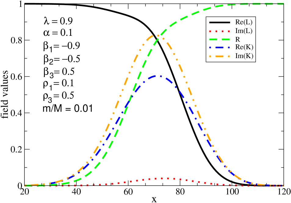
Figure 1: $L$, $R$ and $K$ values for given choice of $\rho_{3}$, $\alpha_{1}$ and $\beta_{1}$, in $M$ units, x values in $M^{-1}$ units. Values of parameters not shown are unity.

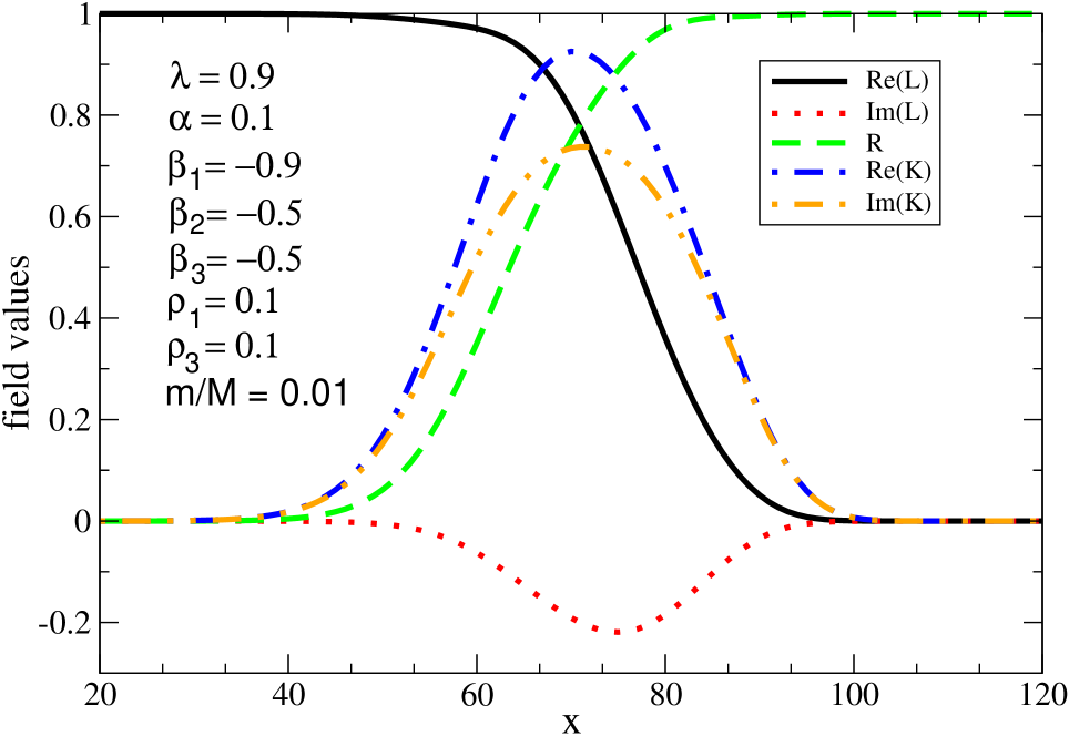
Figure 2: Same as in fig. 1, but for a different choice of $\beta_{1}$.

In addition to the above we need the expression

$${\partial^{2}V\over\partial|K|^{2}} = 2\alpha_{1}(|L|^{2}+R^{2})+2\beta_{1}RL_{1}+2\beta_{2}R\left(L_{1}\cos\alpha-L_{2}\sin\alpha\right)$$

$$+2\beta_{3}R\left(L_{1}\cos 2\alpha-L_{2}\sin 2\alpha\right)+\lambda(3K^{2}+m^{2})$$

for studying stability issues. This shows that to ensure K=0 asymptotically (no E-W breaking at L-R scale) we need

$$2\alpha_{1}+\lambda\left({m\over M}\right)^{2}>0.$$

To obtain $K\neq 0$ in the core of the wall, we again use (V) with the values of $R$ and $L_{1}$ in the core estimated to be $0.5$. This suggests the requirement

$$\lambda K^{2}=-\lambda\left({m\over M}\right)^{2}-\frac{1}{2}\left(2\alpha_{1}+\beta_{1}+\beta_{2}+\beta_{3}\right)>0$$

This has to be revised in view of the actual values of $R$ and $L_{1}$ due to backreaction of the $K$ fields, but serves as a good indicator to the required range of values.

The second equation clearly suggests taking $\beta$’s negative. In particular $\beta_{1}$ can be ${\cal O}(1)$ and negative, which will ensure the required instability of the $K=0$ vacuum inside the wall core. Two examples of numerical solutions are shown in figures 1 and 2. Parameters other than those displayed are taken to be unity. The shape of the $K$ profiles is of the form of the sech function, as expected for lowest linear perturbation in a $\tanh$ background. The numerical study indicates the field profiles are sensitive to the parameters governing the Yukawa couplings, but they have no appreciable variation with respect to the ratio of the mass scales $\left({m\over M}\right)^{2}$.

VI Implications for cosmology

We are now in a position to use the formalism of eqs (13)-(15) to estimate the lepton asymmetry generated. The asymmetry in local number density is given by

$$\Delta n_{\scriptscriptstyle L}\equiv n_{\scriptscriptstyle L}(x)-\bar{n}_{\scriptscriptstyle L}(x)=\frac{1}{6}\,{\mu_{\scriptscriptstyle L}(x)T^{2}}$$ (30)

where $\mu_{\scriptscriptstyle L}$ satisfies the diffusion equation (14). The general form of the solution to this equation is

$$\mu(x) = \left\{\begin{array}[]{ll}B_{\scriptscriptstyle+}{e^{\lambda_{\scriptscriptstyle+}x}}+B_{\scriptscriptstyle-}{e^{\lambda_{\scriptscriptstyle-}x}}+B\int_{-\infty}^{x}dy\,\left[e^{\lambda_{\scriptscriptstyle+}(x-y)}-e^{\lambda_{\scriptscriptstyle-}(x-y)}\right]S(y),&x<0\\ A_{\scriptscriptstyle+}{e^{\rho_{\scriptscriptstyle+}x}}+A_{\scriptscriptstyle-}{e^{\rho_{\scriptscriptstyle-}x}}+\,A\int_{-\infty}^{x}dy\,\left[e^{\rho_{\scriptscriptstyle+}(x-y)}-e^{\rho_{\scriptscriptstyle-}(x-y)}\,\right]S(y),&x>0\end{array}\right.$$ (33)

where

$$\lambda_{\scriptscriptstyle+} = 0,\quad\lambda_{\scriptscriptstyle-}=-{v_{w}\over D},\quad\rho_{\scriptscriptstyle\pm}=-{v_{w}\over 2D}\pm\sqrt{\left({v_{w}\over D}\right)^{2}+{\Gamma_{\rm hf}\over D}}$$ (34)

$$B = {1\over D(\lambda_{\scriptscriptstyle-}-\lambda_{\scriptscriptstyle+})}=-{v_{w}^{-1}},\quad A={1\over D(\rho_{\scriptscriptstyle-}-\rho_{\scriptscriptstyle+})}=-\left({v_{w}^{2}+4\Gamma_{\rm hf}D}\right)^{-1/2}.$$ (35)

The integration constants $A_{\scriptscriptstyle\pm}$ and $B_{\scriptscriptstyle\pm}$ are chosen so that $\mu(x)$ and its derivative are continuous at $x=0$, and $\mu$ is finite as $x\to\pm\infty$. In particular, we are interested in the limiting value $\mu_{0}=\lim_{x\to-\infty}\mu(x)=B_{\scriptscriptstyle+}$, since this is relevant deep within the $L$-like phase and represents the uniform lepton asymmetry filling the universe long after the wall has passed by. It is given by

$$\mu_{0}={1\over v_{w}}\int_{-\infty}^{0}dy\,\left(1+{\rho_{\scriptscriptstyle+}\over\rho_{\scriptscriptstyle-}}e^{v_{w}y/D}\right)S(y)-{1\over\rho_{\scriptscriptstyle-}D}\int_{0}^{\infty}e^{-\rho_{\scriptscriptstyle+}y}S(y).$$ (36)

We note that in the limit $v_{w}\to 0$, the above expression is finite for a generic source $S(y)$. But since our source vanishes when $v_{w}=0$, we get no lepton asymmetry in that limit, which is in accord with Sakharov’s out-of-equilibrium requirement. We can also verify that no lepton asymmetry arises when lepton violating interactions are turned off. For us, this means setting $\Gamma_{\rm hf}=0$, in which case we obtain $\mu_{0}=v_{w}^{-1}\int_{-\infty}^{\infty}S(y)dy$. The integral vanishes if the source itself does not violate global lepton number conservation, so this check also succeeds. The third necessary ingredient, CP violation, is contained within the source $S(y)$, since this depends on the neutrino masses having complex phases which vary within the domain wall.

Now we proceed to estimate the chemical potential $\mu_{0}$ which quantifies the generated lepton asymmetry. This requires the thermal averages cjk2

$$\langle\vec{v}^{2}\rangle = {3x_{\nu}+2\over x_{\nu}^{2}+3x_{\nu}+2}\cong 1;\quad x_{\nu}\equiv{m_{\nu}^{2}(x)\over T^{2}}$$ (37)

$$\left\langle|v_{x}|\over E^{2}\right\rangle \cong {a-bx_{\nu}\over T^{2}};\quad a\cong 0.24;\quad b\cong 0.65$$ (38)

The first approximation (37) is good for relativistic neutrinos with $x_{\nu}\mbox{\raisebox{-2.58334pt}{~{}$\stackrel{{\scriptstyle<}}{{\sim}}$~{}}}0.1$, and the second one (38) is an approximation to the function given in cjk2 which is adequate for our estimate. By taking $\langle\vec{v}^{\,2}\rangle\cong 1$ we can simplify the expression for $\mu_{0}$ since the source $S(y)$ becomes a total derivative. Integrating by parts,

$$\mu_{0}\cong{v_{w}\over T^{2}}\,{\rho_{\scriptscriptstyle+}\over\rho_{\scriptscriptstyle-}}\left[\int_{-\infty}^{0}e^{v_{w}y/D}+\int_{0}^{\infty}e^{-\rho_{\scriptscriptstyle+}y}\right]\left(\left(a-b{m^{2}_{\nu}\over T^{2}}\right)(m^{2}_{\nu}\alpha^{\prime})^{\prime}\right)dy$$ (39)

Since the wall is much thinner than the diffusion scales $D/v_{w}$ and $1/\rho_{\scriptscriptstyle+}$, it is a good approximation to neglect these in the integral (setting $e^{v_{w}y/D}$ and $e^{-\rho_{\scriptscriptstyle+}y}$ to 1). We will use the ansatz $m^{2}_{\nu}(y)=M^{2}_{\scriptscriptstyle N}h^{2}(y)$, $h(y)=\frac{1}{2}(1+\tanh(y/\Delta_{w}))$, for the real part of the neutrino mass, while for the phase, in accordance with the profiles found in the previous section, we take $\alpha(y)={\rm Im}(L(y))/{\rm Re}(L(y))$, with ${\rm Im}(L(y))=\alpha_{0}\Delta_{w}h^{\prime}(y)$. Here $M_{\scriptscriptstyle N}$ is the large value of the neutrino Majorana mass neutrino, acquired by the left (right) -handed neutrino in the $R$-like ($L$-like) phase. We have performed the integral numerically to obtain the analytic result:

$$\Delta n_{\scriptscriptstyle L}\cong 0.08\,v_{w}{\alpha_{0}\over\Delta_{w}}\,{M_{\scriptscriptstyle N}^{4}\over T^{2}}$$ (40)

This is the raw value of the lepton number generated by this mechanism. One would like to express this as a ratio $\eta_{\scriptscriptstyle L}$ of lepton number to entropy as is standard to do with baryon number. Using the expression for the entropy density ${\cal S}=2\pi^{2}g_{*}T^{3}/45$ of $g_{*}$ relativistic degrees of freedom, we get

$$\eta^{\rm raw}_{\scriptscriptstyle L}\cong 0.01\,v_{w}{\alpha_{0}\over g_{*}}\,{M_{\scriptscriptstyle N}^{4}\over T^{5}\Delta_{w}}$$ (41)

Let us consider whether this result can naturally be of the same order as the observed baryon asymmetry. Let $\Delta_{T}$ [as introduced above, eq. (18)] denote the temperature-dependent VEV acquired by the $\Delta_{R}$ in the phase of interest. Experience with the electroweak theory shows that $\Delta_{T}/T$ is determined by the ratio of gauge and Higgs couplings, and is typically smaller than unity. If $f$ is the Yukawa coupling determining the Majorana mass, then $M_{\scriptscriptstyle N}=f\Delta_{T}$. Moreover the inverse wall width $\Delta_{w}^{-1}$ is $\sqrt{\lambda_{\rm eff}}\,\Delta_{T}$, where $\lambda_{\rm eff}$ is the effective quartic self-coupling of the $\Delta$ fields. This is assumed to be small, since we have taken the wall to be thick. Therefore we can reexpress (41) as

$$\eta^{\rm raw}_{\scriptscriptstyle L}\cong 0.01\,v_{w}{\alpha_{0}\over g_{*}}\,\left({\Delta_{T}\over T}\right)^{5}\,f^{4}\,\sqrt{\lambda_{\rm eff}}\ .$$ (42)

With $g_{*}\approx 10^{2}$, this raw lepton asymmetry is close to $\eta_{\scriptscriptstyle B}\cong 10^{-11}$, the desirable value for final baryon asymmetry, provided that

$$\left({\Delta_{T}\over T}\right)^{5}\,f^{4}\,\sqrt{\lambda_{\rm eff}}\approx 10^{-7}\ .$$ (43)

Even if $\Delta_{T}/T\sim O(1)$ and $\sqrt{\lambda_{\rm eff}}\sim 1$, this can be achieved with a reasonable value for the Majorana Yukawa coupling $f_{3}\approx 10^{-2}$ of the heaviest (third generation) sterile neutrino. Ignoring further evolution of the lepton asymmetry for the moment, one could turn this around to derive a lower bound on $f$, assuming that the present mechanism was responsible for baryogenesis. If all the Majorana neutrinos are lighter than $\approx 10^{-2}v_{R}$, then it produces too small a lepton asymmetry to be significant.

After the domain walls have disappeared, the lepton asymmetry undergoes further processing by several interactions. Firstly the electroweak sphalerons will redistribute this asymmetry partially into baryonic form. This is the mechanism by which we get baryon asymmetry from the wall generated lepton asymmetry. The standard chemical equilibrium calculation khlebshap gives

$$\Delta n_{\scriptscriptstyle B}\ =\ \frac{28}{79}\Delta n_{B-L}\ =\ -\frac{28}{51}\Delta n_{\scriptscriptstyle L}$$ (44)

assuming the minimal Higgs and flavour content of the Standard Model.

However the presence of heavy majorana neutrinos gives rise to processes that can deplete the lepton asymmetry generated. Such processes were considered in a model independent way in luty ; Harvey:1990qw ; Fischler:1990gn , referred to in section I. The present model differs from classic GUT scenarios in that the temperature $T_{B-L}=T_{\scriptscriptstyle LR}$ when the lepton asymmetry is created can be less than or comparable to the heavy neutrino mass $M_{\scriptscriptstyle N}$. The two processes of importance are the decay of the heavy neutrino with rate $\Gamma_{\scriptscriptstyle D}$ and heavy neutrino-mediated scattering processes with rate $\Gamma_{\scriptscriptstyle S}$. The latter class of processes in the context of the present model is shown in fig. 3. The rates are given roughly by

$$\Gamma_{\scriptscriptstyle D}\sim{h^{2}M_{\scriptscriptstyle N}^{2}\over 16\pi(4T^{2}+M_{\scriptscriptstyle N}^{2})^{1/2}}\hskip 56.9055pt\Gamma_{\scriptscriptstyle S}\sim{h^{4}\over 13\pi^{3}}{T^{3}\over(9T^{2}+M_{\scriptscriptstyle N}^{2})}$$ (45)

These expressions correctly interpolate between the high and low temperature limits which can be inferred from eqs. (3.1,3.8), (A15-A16) of ref. luty , using the Boltzmann approximation $K_{1}(x)\sim e^{-x}/x$ in the thermal average of the scattering cross section. (The factor $13$ in (45) is really $96\zeta(3)/9$.)

Let us first consider the case when the decays do not deplete the generated lepton asymmetry at all. This happens if the lightest of the heavy majorana neutrinos has $M_{{\scriptscriptstyle N}1}>T_{\scriptscriptstyle LR}$, so that the decays do not occur because of Boltzmann suppression. This limit tends to make the initial lepton asymmetry $\eta_{\scriptscriptstyle L}$ large, possibly $O(1)$ from (41). However the lepton-violating scattering processes will dilute this by the factor $10^{-d_{\scriptscriptstyle L}}\equiv\exp\left(-\int_{t_{\scriptscriptstyle LR}}^{t_{0}}\Gamma_{\scriptscriptstyle S}dt\right)$ where $t_{LR}$ is the time of the LR-breaking phase transition and $t_{0}$ is the present. At the same time, sphalerons will keep the baryon and lepton asymmetries in the same proportion khlebshap until the electroweak phase transition, at which time the sphalerons go out of equilibrium. The corresponding depletion factor for baryons, rewritten in terms of an integral with respect to temperature, is

$$10^{-d_{\scriptscriptstyle B}}\equiv\exp\left(-\int_{T_{\scriptscriptstyle EW}}^{T_{\rm min}}{\Gamma_{\scriptscriptstyle S}\over H}\,{dT\over T}\right);\qquad T_{\rm min}\equiv{\rm min}(T_{\scriptscriptstyle LR},\ T_{\rm sph})$$ (46)

where $T_{\rm sph}\sim 10^{12}$ GeV is the maximum temperature below which sphalerons are in equilibrium. Evaluating the integral gives the baryon depletion exponent

$$d_{\scriptscriptstyle B}\cong{3\sqrt{10}\over 13\pi^{4}\ln 10\sqrt{g_{*}}}\,h^{4}{M_{Pl}T_{\rm min}\,\over M_{\scriptscriptstyle N}^{2}}$$ (47)

where $g_{*}$ is the average number of relativistic degrees of freedom, and we are assuming that $M_{{\scriptscriptstyle N}1}>T_{\rm min}$. Eq. (47) can be solved for the Yukawa coupling $h$ which gives the Dirac mass term for the neutrino: $h^{4}\mbox{\raisebox{-2.58334pt}{~{}$\stackrel{{\scriptstyle<}}{{\sim}}$~{}}}3200\,d_{\scriptscriptstyle B}\left({M_{\scriptscriptstyle N}^{2}\over T_{\rm min}M_{Pl}}\right)$ where we have taken $g_{*}=110$ for definiteness. Since $d_{\scriptscriptstyle B}$ should be no greater than about 10 to avoid too much dilution of the baryon asymmetry, this can be further transformed into an upper limit on the light neutrino masses using the seesaw relation $m_{\nu}=(hv)^{2}/M_{\scriptscriptstyle N}$ where $v$ is the Higgs boson VEV, $v=174$ GeV:

$$m_{\nu}\mbox{\raisebox{-2.58334pt}{~{}$\stackrel{{\scriptstyle<}}{{\sim}}$~{}}}{180v^{2}\over\sqrt{T_{\rm min}M_{Pl}}}\,\left({d_{\scriptscriptstyle B}\over 10}\right)^{1/2}$$ (48)

If the heaviest neutrino mass is $1$ eV, for example, the temperature of the $LR$ phase transition (if it is smaller than $T_{\rm sph}$), being also the temperature at which most of the $B-L$ is generated, is predicted to be

$$T_{B-L}\ =\ T_{\scriptscriptstyle LR}\ \mbox{\raisebox{-2.58334pt}{~{}$\stackrel{{\scriptstyle<}}{{\sim}}$~{}}}10^{13}{\rm\ GeV}\times\left({{\rm\ eV}\over m_{\nu}}\right)^{2}\times\left({d_{\scriptscriptstyle B}\over 10}\right)$$ (49)

Figure 3: The $N$ mediated processes violating $L$

The previous discussion of dilution by lepton-violating scattering assumed the heavy neutrinos $N$ had masses $M_{\scriptscriptstyle N}>T_{\scriptscriptstyle LR}$ so that the decay processes could be neglected. If we are in the opposite regime, $M_{\scriptscriptstyle N}<T_{\scriptscriptstyle LR}$, the decays and inverse decays of $N$ will dominate over scattering for the epoch of temperatures $T>M_{\scriptscriptstyle N}$. For lower temperatures, the decay rate is exponentially suppressed by the Boltzmann factor $e^{-M_{\scriptscriptstyle N}/T}$. We can roughly estimate the dilution due to decays as

$$d_{\scriptscriptstyle B}\ =\ {1\over\ln 10}\int_{M}^{T_{\rm min}}(\Gamma_{D}/H)dT/T\ \cong\ {3\sqrt{10}\over 96\pi^{2}\sqrt{g_{*}}\ln 10}\,h^{2}{M_{Pl}\over M_{\scriptscriptstyle N}}\ \sim 4\times 10^{-4}\ {m_{\nu}M_{Pl}\over v^{2}}$$ (50)

in the limit that $M_{\scriptscriptstyle N}\ll T_{\rm min}$. Again requiring that $d_{\scriptscriptstyle B}<10$ gives the bound on the heaviest neutrino mass

$$m_{\nu}<0.3\ {\rm eV}\times\left({d_{\scriptscriptstyle B}\over 10}\right)$$ (51)

It is interesting that this value is compatible with, and not very far from the value implied by atmospheric neutrino observations.

VII Conclusion

We have shown that a hitherto unexplored mechanism exists in the Left-Right symmetric model for generation of the observed baryon asymmetry of the Universe. The idea is reminiscent of electroweak baryogenesis, but here the motion of domain walls with CP-violating reflections of neutrinos during the LR-breaking phase transition creates a large lepton asymmetry, which is subsequently reprocessed by sphalerons into the baryon asymmetry. Unlike electroweak baryogenesis, there is no suppression by $\alpha_{W}^{4}$, since the sphalerons are in equilibrium and they have sufficient time to equilibrate the baryon and lepton numbers. Rather, the answer is determined to a large extent by $f^{4}$ (see (42)) because asymmetry production is determined by the helicity flipping interactions. There are no natural smallness requirements on this parameter, although through see-saw formula it is constrained by the observed light neutrino mass. Furthermore there are no strong constraints on the CP violating phases since they appear in the interactions of the heavy right handed neutrino.

It is possible to generate the observed baryon asymmetry for a range of parameters of the model. We have studied a few limiting cases to demonstrate the intrinsic potential of this scenario for producing the observed baryon asymmetry. One extreme possibility is that we could start with the raw value of the lepton asymmetry (42) being of order $10^{-10}$ by virtue of a small Majorana Yukawa coupling, eq. (43), while the heaviest left-handed neutrino mass satisfies the bounds (49, 51) (evaluated at $d_{\scriptscriptstyle B}\sim 1$) which guarantee that there is no subsequent dilution of the asymmetry by lepton-violating interactions. The other limiting case is to initially create an asymmetry of $O(1)$, by taking large Majorana Yukawa couplings; the asymmetry is subsequently diluted to the required level by saturating the bounds (49, 51), which make reference to the heaviest left-handed neutrino mass.

An interesting application of this mechanism is the possibility to generate a large lepton number as suggested in Harvey:1981cu and considered in the context of new observations in cosmology e.g. in Rowan-Robinson:2000ys -LL , notably the MAP and PLANCK experiments to measure the cosmic microwave background (CMB) fluctuations. In the simplest model with just one lepton generation, we cannot create a large lepton asymmetry without also making the baryon asymmetry too large. But consider a model with a certain combination of lepton numbers conserved, such as $L_{e}+L_{\mu}$. This would be the case if the Majorana mass matrix had the form $({0\ M\atop M\ 0})$. Then the leptogenesis mechanism would create equal and opposite amounts of $L_{e}$ and $L_{\mu}$. Since sphalerons separately conserve $\frac{1}{3}B-L_{e}$ and $\frac{1}{3}B-L_{\mu}$, the combination $\frac{2}{3}B-L_{e}-L_{\mu}$ would remain conserved at all times, so that the resulting baryon asymmetry would be zero even if $|L_{e}|$ and $|L_{\mu}|$ separately were large. By adding a very small breaking of the $L_{e}+L_{\mu}$ symmetry, one could generate the observed baryon asymmetry simlutaneously with large lepton asymmetries MR . In addition to its imprint on the CMB, such an effect could have other observable consequences as observations relevant to nucleosynthesis are improved Shi -sarkar .

Appendix A: minimization conditions for wall profiles

These conditions for finding the wall profiles were used in section IV.2

$${\delta V\over\delta v_{\scriptscriptstyle L}} = \frac{1}{2}\{\alpha_{1}k_{1}^{2}v_{\scriptscriptstyle L}+\alpha_{1}k_{2}^{2}v_{\scriptscriptstyle L}+\alpha_{3}k_{2}^{2}v_{\scriptscriptstyle L}-2\mu_{3}^{2}v_{\scriptscriptstyle L}$$ (52)

$$+ 2\rho_{1}v_{\scriptscriptstyle L}^{3}+\rho_{3}v_{\scriptscriptstyle L}v_{\scriptscriptstyle R}^{2}+4\alpha_{2}k_{1}k_{2}v_{\scriptscriptstyle L}\cos(\alpha)$$

$$+ \beta_{1}k_{1}k_{2}v_{\scriptscriptstyle R}\cos(\alpha-\theta)+\beta_{2}k_{1}^{2}v_{\scriptscriptstyle R}\cos(2\alpha-\theta)+\beta_{3}k_{2}^{2}v_{\scriptscriptstyle R}\cos(\theta)\}$$

$${\delta V\over\delta v_{\scriptscriptstyle R}} = \frac{1}{2}\{\alpha_{1}k_{1}^{2}v_{\scriptscriptstyle R}+\alpha_{1}k_{2}^{2}v_{\scriptscriptstyle R}+\alpha_{3}k_{2}^{2}v_{\scriptscriptstyle R}$$ (53)

$$- 2\mu_{3}^{2}v_{\scriptscriptstyle R}+\rho_{3}v_{\scriptscriptstyle L}^{2}v_{\scriptscriptstyle R}+2\rho_{1}v_{\scriptscriptstyle R}^{3}$$

$$+ 4\alpha_{2}k_{1}k_{2}v_{\scriptscriptstyle R}\cos(\alpha)+\beta_{1}k_{1}k_{2}v_{\scriptscriptstyle L}\cos(\alpha-\theta)$$

$$+ \beta_{2}k_{1}^{2}v_{\scriptscriptstyle L}\cos(2\alpha-\theta)+\beta_{3}k_{2}^{2}v_{\scriptscriptstyle L}\cos(\theta)\}$$

$${\delta V\over\delta\theta} = -\frac{1}{2}v_{\scriptscriptstyle L}v_{\scriptscriptstyle R}\{-\beta_{1}k_{1}k_{2}\sin(\alpha-\theta)-\beta_{2}k_{1}^{2}\sin(2\alpha-\theta)+\beta_{3}k_{2}^{2}\sin\theta\}$$ (54)

$${\delta V\over\delta k_{2}} = \lambda_{1}(k_{1}^{2}k_{2}+k_{2}^{3})+2\lambda_{3}k_{1}^{2}k_{2}$$ (55)

$$- \mu_{1}^{2}k_{2}+\frac{1}{2}\alpha_{1}k_{2}v_{\scriptscriptstyle L}^{2}+\frac{1}{2}\alpha_{3}k_{2}v_{\scriptscriptstyle L}^{2}$$

$$+ \frac{1}{2}\alpha_{1}k_{2}v_{\scriptscriptstyle R}^{2}+\frac{1}{2}\alpha_{3}k_{2}v_{\scriptscriptstyle R}^{2}+k_{1}^{3}\lambda_{4}\cos\alpha$$

$$+ 3k_{1}k_{2}^{2}\lambda_{4}\cos\alpha-2k_{1}\mu_{2}^{2}\cos\alpha+\alpha_{2}k_{1}v_{\scriptscriptstyle L}^{2}\cos\alpha+\alpha_{2}k_{1}v_{\scriptscriptstyle R}^{2}\cos\alpha$$

$$+ 4k_{1}^{2}k_{2}l\alpha_{2}\cos 2\alpha+\frac{1}{2}\beta_{1}k_{1}v_{\scriptscriptstyle L}v_{\scriptscriptstyle R}\cos(\alpha-\theta)+\beta_{3}k_{2}v_{\scriptscriptstyle L}v_{\scriptscriptstyle R}\cos\theta$$

$${\delta V\over\delta k_{1}} = k_{1}^{3}\lambda_{1}+k_{1}k_{2}^{2}\lambda_{1}+2k_{1}k_{2}^{2}\lambda_{3}-k_{1}\mu_{1}^{2}$$ (56)

$$+ \frac{1}{2}\alpha_{1}k_{1}v_{\scriptscriptstyle L}^{2}+\frac{1}{2}\alpha_{1}k_{1}v_{\scriptscriptstyle R}^{2}+3k_{1}^{2}k_{2}\lambda_{4}\cos(\alpha)$$

$$+ k_{2}^{3}\lambda_{4}\cos(\alpha)-2k_{2}\mu_{2}^{2}\cos(\alpha)+\alpha_{2}k_{2}v_{\scriptscriptstyle L}^{2}\cos(\alpha)$$

$$+ \alpha_{2}k_{2}v_{\scriptscriptstyle R}^{2}\cos(\alpha)+4k_{1}k_{2}^{2}\lambda_{2}\cos(2\alpha)+\frac{1}{2}\beta_{1}k_{2}v_{\scriptscriptstyle L}v_{\scriptscriptstyle R}\cos(\alpha-\theta)$$

$$+ \beta_{2}k_{1}v_{\scriptscriptstyle L}v_{\scriptscriptstyle R}\cos(2\alpha-\theta)$$

$${\delta V\over\delta\alpha} = -\lambda_{4}k_{1}k_{2}(k_{1}^{2}+k_{2}^{2})\sin\alpha+2k_{1}k_{2}\mu_{2}^{2}\sin\alpha$$ (57)

$$- \alpha_{2}k_{1}k_{2}(v_{\scriptscriptstyle L}^{2}+v_{\scriptscriptstyle R}^{2})\sin(\alpha)-4k_{1}^{2}k_{2}^{2}\lambda_{2}\sin 2\alpha-\frac{1}{2}\beta_{1}k_{1}k_{2}v_{\scriptscriptstyle L}v_{\scriptscriptstyle R}\sin(\alpha-\theta)$$

$$- \beta_{2}k_{1}^{2}v_{\scriptscriptstyle L}v_{\scriptscriptstyle R}\sin(2\alpha-\theta)$$

References

• (1) M. E. Shaposhnikov, Nucl. Phys. B 287, 757 (1987). JETP Lett.  44, 465 (1986) [Pisma Zh. Eksp. Teor. Fiz.  44, 364 (1986)]. Phys. Lett. B 277, 324 (1992) [Erratum-ibid. B 282, 483 (1992)].
G. R. Farrar and M. E. Shaposhnikov, Phys. Rev. Lett.  70, 2833 (1993) [Erratum-ibid.  71, 210 (1993)] [arXiv:hep-ph/9305274]. Phys. Rev. D 50, 774 (1994) [arXiv:hep-ph/9305275].
• (2) A. G. Cohen, D. B. Kaplan and A. E. Nelson, Phys. Lett. B 245, 561 (1990). Nucl. Phys. B 349, 727 (1991). Phys. Lett. B 263, 86 (1991). Nucl. Phys. B 373, 453 (1992). Phys. Lett. B 294, 57 (1992) [arXiv:hep-ph/9206214].
• (3) M. Joyce, T. Prokopec and N. Turok, Phys. Rev. D 53, 2930 (1996) [arXiv:hep-ph/9410281].
P. Huet and A. E. Nelson, Phys. Lett. B 355, 229 (1995) [arXiv:hep-ph/9504427]; Phys. Rev. D 53, 4578 (1996) [arXiv:hep-ph/9506477]. J. M. Cline, K. Kainulainen and A. P. Vischer, Phys. Rev. D 54, 2451 (1996)
• (4) S. Ben-Menahem and A. S. Cooper, Nucl. Phys. BB388, 409 (1992)
• (5) S. Bhowmik Duari and U. A. Yajnik, Phys. Lett. B326 21 (1994)
• (6) R. Brandenberger, A-C. Davis, and M. Trodden, Phys. Lett. B335 123 (1994)
• (7) R. Mohapatra and X. Zhang, Phys. Rev. D46, 5331 (1992)
• (8) J. M. Frere, L. Houart, J. M. Moreno, J. Orloff and M. Tytgat, Phys. Lett. B 314, 289 (1993)
• (9) H. Lew and A. Riotto, Phys. Lett. B309, 258 (1993)
• (10) U. A. Yajnik, H. Widyan, S. Mahajan, A. Mukherjee and D. Choudhuri Phys. Rev. D59 (1999) 103508
• (11) M. Fukugita and T. Yanagida, Phys. Lett. B174 45 (1986)
• (12) M. Luty, Phys. Rev. D45 455 (1992)
• (13) M. Plumacher, Z. Phys. C 74 549 (1997)
• (14) W. Buchmuller and M. Plumacher, hep-ph/9711208, $4^{th}$ Paris Cosmology Colloquium, 1997
• (15) J. A. Harvey and M. S. Turner, Phys. Rev. D 42, 3344 (1990).
• (16) W. Fischler, G. F. Giudice, R. G. Leigh and S. Paban, Phys. Lett. B 258, 45 (1991).
• (17) See the review W. Buchmuller and M. Plumacher, Int. J. Mod. Phys. A 15, 5047 (2000) [arXiv:hep-ph/0007176] and references therein.
• (18) R. N. Mohapatra and G. Senjanovic, Phys. Rev. Lett. 44, 912 (1980), Phys. Rev. D23, 165 (1981).
• (19) R. N. Mohapatra, Unification And Supersymmetry (Springer-Verlag, New York, 1992).
• (20) N. G. Deshpande, J. F. Gunion, B. Kayser and F. Olness, Phys. Rev. D44, 3320 (1991).
• (21) G. Barenboim and J. ${\rm Bernab\acute{e}u}$, Z. Phys. C 73, 321 (1997).
• (22) M. Joyce, T. Prokopec and N. Turok, Phys. Rev. Lett.  75, 1695 (1995); Erratum-ibid.75, 3375 (1995); Phys. Rev.  D53, 2958 (1996).
• (23) J. Cline, M. Joyce and K. Kainulainen Phys. Rev. Lett. 85, 5519 (2000) Phys. Lett. B417 79 (1998) [Erratum-ibid. B 448, 321 (1998)] [hep-ph/9708393].
• (24) J. Cline and K. Kainulainen Phys. Rev. Lett. 85, 5519 (2000)
• (25) S. A. Abel, S. Sarkar and P. L. White, Nucl. Phys. B 454, 663 (1995) [arXiv:hep-ph/9506359].
• (26) S. E. Larsson, S. Sarkar and P. L. White, Phys. Rev. D 55, 5129 (1997) [arXiv:hep-ph/9608319].
• (27) Summarised in the cosmological context in T. W. Kibble, in C80-02-18.1.2 Phys. Rept.  67, 183 (1980).
• (28) J. M. Cline, M. Joyce and K. Kainulainen, JHEP 0007, 018 (2000) [arXiv:hep-ph/0006119]. [erratum: arXiv:hep-ph/0110031]
• (29) S. Yu. Khlebnikov and M. E. Shaposhnikov, Nucl. Phys. B308 885 (1988).
Also reviewed in buchplum .
• (30) J. A. Harvey and E. W. Kolb, Phys. Rev. D 24, 2090 (1981).
• (31) M. Rowan-Robinson, in The Identification of dark matter : Proceedings, Neil J. C. Spooner and Vitaly Kudryavtsev, ed.s, World Scientific Pub. Co. 2001. [arXiv:astro-ph/0012026].
• (32) A. D. Dolgov, S. H. Hansen, S. Pastor, S. T. Petcov, G. G. Raffelt and D. V. Semikoz, Nucl. Phys. B 632, 363 (2002) [arXiv:hep-ph/0201287].
• (33) W. H. Kinney and A. Riotto, Phys. Rev. Lett.  83, 3366 (1999)
• (34) T. Kajino, M. Orito, G. J. Mathews and R. N. Boyd, arXiv:astro-ph/0202114.
• (35) J. Lesgourgues and A. R. Liddle, Mon. Not. Roy. Astron. Soc.  327, 1307 (2001) [arXiv:astro-ph/0105361].
• (36) J. March-Russell, H. Murayama and A. Riotto, JHEP 9911, 015 (1999) [arXiv:hep-ph/9908396].
• (37) X. d. Shi, G. M. Fuller and K. Abazajian, Phys. Rev. D 60, 063002 (1999) [arXiv:astro-ph/9905259].
• (38) D. P. Kirilova and M. V. Chizhov, Nucl. Phys. B 534, 447 (1998)
• (39) S. Sarkar, in proceedings of ”DARK98” Heidelberg, Germany, 1998, [arXiv:astro-ph/9903183].