Cabibbo allowed $D\to K\pi\gamma$ decays

S. Fajfer^a,b, A. Prapotnik^b and P. Singer^c

a) Department of Physics, University of Ljubljana, Jadranska 19, 1000 Ljubljana, Slovenia

b) J. Stefan Institute, Jamova 39, P. O. Box 300, 1001 Ljubljana, Slovenia

c) Department of Physics, Technion - Israel Institute of Technology, Haifa 32000, Israel

ABSTRACT

The weak radiative Cabibbo allowed decays $D^{+}\to{\bar{K}}^{0}\pi^{+}\gamma$ and $D^{0}\to K^{-}\pi^{+}\gamma$ with nonresonant $K\pi$ are investigated by relying on the factorization approximation for the nonleptonic weak transitions and the model which combines the heavy quark effective theory and the chiral Lagrangian approach. The dominant contributions to the amplitudes come from the long distance effects. The decay amplitude has both parity violating and parity conserving parts. The parity violating part includes also a bremsstrahlung contribution. The branching ratio obtained for the parity conserving part is of the order $10^{-4}$ for the $D^{0}\to K^{-}\pi^{+}\gamma$ decay and $10^{-5}$ for $D^{+}\to{\bar{K}}^{0}\pi^{+}\gamma$, when the effect of light vector mesons is included, and smaller otherwise. The branching ratio for the parity violating part with a photon energy cut of $50$ ${\rm MeV}$, is close to $10^{-3}$ for the $D^{0}$ decay and $4\times 10^{-4}$ for the $D^{+}$ decay. We present Dalitz plots and energy spectra for both transitions as derived from our model and we probe the role of the light vector mesons in these decays.

I. INTRODUCTION

The investigation of radiative and dilepton weak decays of pseudoscalar charm mesons has been pursued rather vigorously in recent years, both theoretically and experimentally. To a certain extent, this activity has been fueled by the ongoing search for physics beyond the standard model, which might be of measurable consequence in certain charm radiative and dilepton decays [1-4]. To date, no radiative or dilepton weak decay of $D$ has been detected. However, upper bounds have been established for a sizable number of these decays. The radiative decays $D^{0}\to\rho^{0},$ $\omega^{0},$ $\phi,$ $\bar{K}^{*0}$ $+\gamma$ were recently bounded [5] to branching ratios in the $10^{-4}$ range, which is approaching the standard model expectations (see, e.g. [6, 7] where additional previous works are mentioned). The dilepton decays $D\to Pl^{+}l^{-}$, $D\to Vl^{+}l^{-}$ are the subject of intensive searches at CLEO and Fermilab [8]. Here again, with upper bounds of $10^{-5}-10^{-4}$ for branching ratios of the various modes one approaches the expectations of the standard model [2, 3, 4, 9]. The situation should improve in the future, due to new possibilities for observation of charm meson decays at BELLE, BABAR and Tevatron. Recently, upper limits in the $10^{-5}-10^{-4}$ range were established [10] also for $D^{0}$ dilepton decays with two nonresonant pseudoscalar mesons in the final state $D^{0}\to(\pi^{+}\pi^{-},K^{-}\pi^{+},K^{+}K^{-})$ $\mu^{+}\mu^{-}$, though no comparable results are available yet for similar photonic decays.

In the present work, we undertake the study of the Cabibbo allowed radiative decays $D^{+}\to{\bar{K}}^{0}\pi^{+}\gamma$ and $D^{0}\to K^{-}\pi^{+}\gamma$, which we consider to be the most likely candidates for early detection. These decays are the charm sector counterpart of the $K\to\pi\pi\gamma$ [11, 12, 13] decays, which have provided a wealth of information on meson dynamics. In the strange sector, the $K^{+}\to\pi^{+}\pi^{0}\gamma$ and $K_{L}\to\pi^{+}\pi^{-}\gamma$ are singled out as the most suitable ones for the investigation of the radiative decay mechanism; this, since the relative suppresion of the corresponding $K^{+}\to\pi^{+}\pi^{0}$ and $K_{L}\to\pi^{+}\pi^{-}$ amplitudes leads to a situation where the direct radiative transition is not overwhelmed by the bremsstrahlung part.

In the $K\to\pi\pi\gamma$ decays, the long - distance contribution is dominant [13]. In the charm radiative decays, the theoretical studies show that likewise, the long - distance is the dominant feature of the decays [2, 4, 6, 7, 9]. The short - distance contribution realized by the penguin diagram $c\to u\gamma$ [14, 15, 16] might play a role in certain Cabibbo suppressed decays, which are not discussed in the present paper.

In the charm sector, the nonleptonic D meson decays still provide a continuing theoretical challenge (see, e.g. [17, 18] and references therein). The short distance effects are considered well understood but the perturbative techniques required for the evaluation of certain matrix elements are based on approximate models. Usually the factorization approximation is used (see, e.g. [17, 19]), although the experimental data indicate the apparent need for the inclusion of nonfactorizable amplitudes in certain channels.

In this first treatment of $D\to K\pi\gamma$ decays we use the factorization approximation for the calculation of weak transition elements. We consider the use of this approach to be justified by the ”near” success of the approach for the nonleptonic amplitudes. This will involve its use in the $D(D^{*})K\pi$ vertices as well as in $D(D^{*})\to V$ and $D(D^{*})\to P$ transitions, all of which required for the calculations of the $D\to K\pi\gamma$ amplitudes within our model. For the evaluation of the $(D,D^{*})\to(P,V)$ transitions, we use the information obtained for these matrix elements from semileptonic decays (see, e.g. [20]). The general theoretical framework for our calculation is that of the heavy quark chiral Lagrangian [21, 22]. In the $K\to\pi\pi\gamma$ decays, it has been shown that intermediate light vector mesons play an important role in the decay amplitude [11]. We shall investigate the role of intermediate light vector mesons also in the $D\to K\pi\gamma$ amplitude. In order to accomplish this, we use the extension of the formalism of [21, 22] to include also the light vector mesons [23, 24].

The present study of $D^{+}\to{\bar{K}}^{0}\pi^{+}\gamma$ and $D^{0}\to K^{-}\pi^{+}\gamma$ shows that the direct part of the radiative amplitude is not much smaller in strength than the bremsstrahlung part, rather similarly to the inhibited K decays mentioned above. If confirmed by experiments, it places these decays in the status of a most suitable ground for the investigation of the mechanisms involved in such nonleptonic D decays.

In Section II we present the theoretical framework for our calculation. In Section III we display the explicit expressions of all the calculated decay amplitudes. Section IV contains the discussion and the summary.

II. THE THEORETICAL FRAMEWORK

The nonradiative two-body D - decays, from which the bremsstrahlung part of the radiative decays originates, are $D^{0}\to K^{-}\pi^{+}$ and $D^{+}\to\bar{K}^{0}\pi^{+}$. The weak $\Delta I=1$ transition leads to two independent isospin amplitudes in the final state, $A_{1/2}$ and $A_{3/2}$ and the relations to the physical decays is [18]

$$A(D^{+}\to\bar{K}^{0}\pi^{+})=A_{3/2};\enspace A(D^{0}\to K^{-}\pi^{+})=\frac{2}{3}A_{1/2}+\frac{1}{3}A_{3/2}.$$ (1)

From the determined branching ratios [25] of $BR(D^{+}\to\bar{K}^{0}\pi^{+})=(2.89\pm 0.26)\%$ and $BR(D^{0}\to K^{-}\pi^{+})=(3.83\pm 0.09)\%$ one learns that the relative size of the absolute values of the amplitudes $|A(D^{0}\to K^{-}\pi^{+})|/|A(D^{+}\to\bar{K}^{0}\pi^{+})|$ is $1.84$. Using also the information from the third decay, $A(D^{0}\to\bar{K}^{0}\pi^{0})$ $=\frac{{\sqrt{2}}}{3}A_{1/2}-\frac{{\sqrt{2}}}{3}A_{3/2}$, the isospin analysis shows that $|A_{1/2}|/|A_{3/2}|\simeq 2.7$, and their relative phase is $90^{o}$ [26]. Despite this knowledge, there is still no complete interpretation for the mechanisms leading to the decays [26], although it is clear that the situation is different from the $K\to\pi\pi$ channels, where $\Delta I=1/2$ enhancement introduces a large disparity between the final state isospin amplitudes. The relevance of the above picture to the radiative decays will be discussed in the last Section.

Since our problem of describing the $D\to K\pi\gamma$ decays involves transitions between heavy mesons and light pseudoscalars, we adopt the effective Lagrangian [21, 22] which contains both the heavy flavor and the $SU(3)_{L}\times SU(3)_{R}$ chiral symmetry as the theoretical framework for our calculation. From the experience with $K\to\pi\pi\gamma$ decays, one knows [11, 12, 13] that the decay amplitude is largely determined by contributions from virtual vector mesons. Considering the possibilty that vector mesons would play a role in the $D\to K\pi\gamma$ decays as well (we remind the reader that we consider here nonresonant $K\pi$, the decays $D\to K^{*}\gamma$ having been treated separately [16, 27]), we should complement the Lagrangian by introducing light vector mesons. For this we choose the generalization of the original Lagrangian [21, 22] by Casalbuoni et al [23] in which the original symmetry is broken spontaneously to diagonal $SU(3)_{V}$ [28] with the introduction of the light vector mesons. We present here in some detail this formalism (for more details see [27]), which we use as the main tool of our calculation. We shall perform the calculations also without vector mesons in the Lagrangian in which case the original heavy quark chiral Lagrangian [21, 22] is used, in order to clarify their role in these decays.

The light degrees of freedom are described by the 3$\times$3 Hermitian matrices

$$\Pi=\pmatrix{{\pi^{0}\over\sqrt{2}}+{\eta_{8}\over\sqrt{6}}+{\eta_{0}\over\sqrt{3}}&\pi^{+}&K^{+}\cr\pi^{-}&{-\pi^{0}\over\sqrt{2}}+{\eta_{8}\over\sqrt{6}}+{\eta_{0}\over\sqrt{3}}&K^{0}\cr K^{-}&{\bar{K}^{0}}&-{2\eta_{8}\over\sqrt{6}}+{\eta_{0}\over\sqrt{3}}\cr}$$ (2)

and

$$\rho_{\mu}=\pmatrix{{\rho^{0}_{\mu}+\omega_{\mu}\over\sqrt{2}}&\rho^{+}_{\mu}&K^{*+}_{\mu}\cr\rho^{-}_{\mu}&{-\rho^{0}_{\mu}+\omega_{\mu}\over\sqrt{2}}&K^{*0}_{\mu}\cr K^{*-}_{\mu}&{\bar{K}^{*0}}_{\mu}&\Phi_{\mu}\cr}$$ (3)

for the pseudoscalar and vector mesons, respectively. They are usually expressed through the combinations

$$u = \exp\left(\frac{i\Pi}{f}\right)\;,$$ (4)

where $f\simeq f_{\pi}=132$ MeV is the pion pseudoscalar decay constant, and

$${\hat{\rho}}_{\mu} = i{g_{v}\over\sqrt{2}}\rho_{\mu}\;,$$ (5)

where $g_{v}=5.9$ was fixed in the case of exact flavor symmetry [28]. In the following we will also use the gauge field tensor $F_{\mu\nu}({\hat{\rho}})$

$$F_{\mu\nu}({\hat{\rho}})=\partial_{\mu}{\hat{\rho}}_{\nu}-\partial_{\nu}{\hat{\rho}}_{\mu}+[{\hat{\rho}}_{\mu},{\hat{\rho}}_{\nu}].$$ (6)

It is convenient to introduce two currents ${\cal V}_{\mu}=\frac{1}{2}(u^{{\dagger}}D_{\mu}u+uD_{\mu}u^{{\dagger}})$ and ${\cal A}_{\mu}=\frac{1}{2}(u^{{\dagger}}D_{\mu}u-uD_{\mu}u^{{\dagger}})$. The covariant derivative of $u$ and $u^{{\dagger}}$ is defined as $D_{\mu}u=(\partial_{\mu}+{\hat{B}}_{\mu})u$ and $D_{\mu}u^{{\dagger}}=(\partial_{\mu}+{\hat{B}}_{\mu})u^{{\dagger}}$, with ${\hat{B}}_{\mu}=ieB_{\mu}Q$, $Q=diag(2/3,-1/3,-1/3)$, $B_{\mu}$ being the photon field.

The light meson part of the strong Lagrangian can be written as [28]

$${\cal L}_{light} = -{f^{2}\over 2}\{tr({\cal A}_{\mu}{\cal A}^{\mu})+a\,tr[({\cal V}_{\mu}-{\hat{\rho}}_{\mu})^{2}]\}$$ (7)

$$+ {1\over 2g_{v}^{2}}tr[F_{\mu\nu}({\hat{\rho}})F^{\mu\nu}({\hat{\rho}})]\;.$$

The constant $a$ in (7) is in principle a free parameter. In the case of exact vector meson dominance (VDM) $a=2$ [28, 29]. However, the photo production and decays data indicate [30] that the $SU(3)$ breaking modifies the VDM in

$${\cal L}_{V-\gamma}=-eg_{v}f^{2}B_{\mu}(\rho^{0\mu}+\frac{1}{3}\omega^{\mu}-\frac{{\sqrt{2}}}{3}\Phi^{\mu}).$$ (8)

Instead of the exact $SU(3)$ limit ($g_{v}=m_{V}/f$), we shall use the measured values, defining

$$<V(\epsilon_{V},q)|V_{\mu}|0>=i\epsilon_{\mu}^{*}(q)g_{V}(q^{2}).$$ (9)

The couplings $g_{V}(m_{V}^{2})$ are obtained from the leptonic decays of these mesons. In our calculation we use $g_{\rho}(m_{\rho}^{2})\simeq g_{\rho}(0)=0.17GeV^{2}$, $g_{\omega}(m^{2}_{\omega})\simeq g_{\omega}(0)=0.15GeV^{2}$ and $g_{\Phi}(m^{2}_{\Phi})\simeq g_{\Phi}(0)=0.24GeV^{2}$.

Both the heavy pseudoscalar and the heavy vector mesons are incorporated in a $4\times 4$ matrix

$$H_{a} = \frac{1}{2}(1+\!\!\not{\!v})(P_{a\mu}^{*}\gamma^{\mu}-P_{a}\gamma_{5})\;,$$ (10)

where $a=1,2,3$ is the $SU(3)_{V}$ index of the light flavors, and $P_{a\mu}^{*}$, $P_{a}$, annihilate a spin $1$ and spin $0$ heavy meson $Q\bar{q}_{a}$ of velocity $v$, respectively. They have a mass dimension $3/2$ instead of the usual $1$, so that the Lagrangian is in the heavy quark limit $m_{Q}\to\infty$ explicitly mass independent. Defining moreover

$${\bar{H}}_{a} = \gamma^{0}H_{a}^{{\dagger}}\gamma^{0}=(P_{a\mu}^{*{\dagger}}\gamma^{\mu}+P_{a}^{{\dagger}}\gamma_{5})\frac{1}{2}(1+\!\!\not{\!v})\;,$$ (11)

we can write the strong Lagrangian as [24]

$${\cal L}_{even} = {\cal L}_{light}+iTr(H_{a}v_{\mu}D^{\mu}{\bar{H}}_{a})$$ (12)

$$+ igTr[H_{b}\gamma_{\mu}\gamma_{5}({\cal A}^{\mu})_{ba}{\bar{H}}_{a}]+i{\tilde{\beta}}Tr[H_{b}v_{\mu}({\cal V}^{\mu}-{\hat{\rho}}_{\mu})_{ba}{\bar{H}}_{a}]\;,$$

where $D^{\mu}{\bar{H}}_{a}=(\partial_{\mu}+{\cal V}_{\mu}-ieQ^{\prime}B_{\mu}){\bar{H}}_{a}$, with $Q^{\prime}=2/3$ for c quark.

The coupling $g$ can be fixed [31] by using the data [32] on $D^{*}\to D\pi$ decay width. These data give $g=0.59$. The plus sign is taken to be in agreement with the quark model studies. The parameter ${\tilde{\beta}}$ is less known, but it seems that it can be safely neglected [17].

The electromagnetic field can couple to the mesons also through the anomalous interaction; i.e., through the odd parity Lagrangian. The contributions to this Lagrangian arise from terms of the Wess - Zumino - Witten kind, given by [29, 33]

$${\cal L}^{(1)}_{odd} = -4\frac{C_{VV\Pi}}{f}\epsilon^{\mu\nu\alpha\beta}Tr(\partial_{\mu}{\rho}_{\nu}\partial_{\alpha}{\rho}_{\beta}\Pi).$$ (13)

The coupling $C_{VV\Pi}$ can be determined in the case of the exact $SU(3)$ flavor symmetry following the hidden symmetry approach of [28, 29] and it is found to be $C_{VV\Pi}=3g_{v}^{2}/32\pi^{2}=0.33$. In the actual calculation, we allowed for $SU(3)$ symmetry breaking and we used the $VP\gamma$ coupling as determined from experiment [25]. We will also need the odd - parity Lagrangian in the heavy sector. Such terms are required by the $D^{*}\to D\gamma$ transition, which cannot be generated from (12). There are two contributions [24, 34] in it, characterized by coupling strengths $\lambda$ and $\lambda^{\prime}$. The first is given by

$${\cal L}_{1} = i{\lambda}Tr[H_{a}\sigma_{\mu\nu}F^{\mu\nu}(\hat{\rho})_{ab}{\bar{H}_{b}}].$$ (14)

In this term the interactions of light vector mesons with heavy pseudoscalar or heavy vector mesons is described. The light vector meson can then couple to the photon by the standard VDM prescription. This term is of the order ${1}/{{\lambda}_{\chi}}$ with ${\lambda}_{\chi}$ being the chiral perturbation theory scale [35].

The second term gives the direct heavy quark - photon interaction and is generated by the Lagrangian

$${\cal L}_{2} = -{\lambda}^{\prime}Tr[H_{a}\sigma_{\mu\nu}F^{\mu\nu}(B){\bar{H}_{a}}].$$ (15)

The parameter ${\lambda}^{\prime}$ is given in heavy quark symmetry limit by ${\lambda}^{\prime}\simeq-1/(6m_{c})$ [22] and it should be considered as a higher order term in $1/m_{Q}$ expansion [36].

In order to gain information on these couplings one has to use the existing data on $D^{*0}\to D^{0}\gamma$, $D^{*+}\to D^{+}\gamma$ and $D_{s}^{*+}\to D^{+}_{s}\gamma$ decays. Experimentally, the ratios $R_{\gamma}^{0}=\Gamma(D^{*0}\to D^{0}\gamma)/\Gamma(D^{*0}\to D^{0}\pi^{0})$ and $R_{\gamma}^{+}=\Gamma(D^{*+}\to D^{+}\gamma)/\Gamma(D^{*+}\to D^{+}\pi^{0})$ are known [25]. These data determine two possibilities [27]. One of them is $|\lambda/g|=0.839$ $GeV^{-1}$, $|\lambda^{\prime}/g|=0.175$ $GeV^{-1}$. The second one does not agree with present data. With $g=0.59$ we obtain $\lambda=\pm 0.49$ $GeV^{-1}$ and $\lambda^{\prime}=\pm 0.102$ $GeV^{-1}$.

The $\lambda^{\prime}\simeq-1/(6m_{c})$ would give with the mass of charm quark $m_{c}=1.4$ $GeV$ that $\lambda^{\prime}=-0.12$ $GeV^{-1}$, in good agreement with the above value. The simple quark model analysis indicates that $\lambda^{\prime}$ and $\lambda$ are both negative [36]. In our numerical calculations we give the results using these parameters. In the literature (e.g. [31, 36, 37]) instead of $\lambda$ the $\beta$ parameter is often used. The value $\beta=2.3$ $GeV^{-1}$ corresponds to $\lambda=-0.49$ $GeV^{-1}$, since $2\lambda\frac{g_{v}}{{\sqrt{2}}}$ $(g_{\rho}/m_{\rho}^{2}+g_{\omega}/(3m_{\omega}^{2}))=-(2/3)\beta$.

In addition to strong and electromagnetic interactions, we have to specify the weak one. The nonleptonic weak Lagrangian on the quark level for the Cabibbo allowed decays can be written as usual [19]

$${\cal L}_{NL}^{eff}(\Delta c=\Delta s=1) = -{G_{F}\over\sqrt{2}}V_{ud}V_{cs}^{*}[a_{1}O_{1}+a_{2}O_{2}],$$ (16)

where $O_{1}=({\bar{u}}d)^{\mu}_{V-A}({\bar{s}}c)_{V-A,\mu}$ and $O_{2}=({\bar{u}}c)_{V-A,\mu}({\bar{s}}d)_{V-A}^{\mu}$, $V_{ij}$ are the CKM matrix elements, $G_{F}$ is the Fermi constant and $({\bar{\Psi}}_{1}\Psi_{2})^{\mu}\equiv{\bar{\Psi}}_{1}\gamma^{\mu}(1-\gamma^{5})\Psi_{2}$. In our calculation we use $a_{1}=1.26$ and $a_{2}=-0.55$ as found in [19].

At the hadronic level, the weak current transforms as $({\bar{3}}_{L},1_{R})$ under chiral $SU(3)_{L}\times SU(3)_{R}$, is linear in the heavy meson fields $D^{a}$ and $D^{*a}_{\mu}$ and is taken as [20]

$${J_{Q}}_{a}^{\mu}= \frac{1}{2} i\alpha Tr[\gamma^{\mu}(1-\gamma_{5})H_{b}u_{ba}^{{\dagger}}]$$ (17)

$$+ \alpha_{1}Tr[\gamma_{5}H_{b}({\hat{\rho}}^{\mu}-{\cal V}^{\mu})_{bc}u_{ca}^{{\dagger}}]$$

$$+ \alpha_{2}Tr[\gamma^{\mu}\gamma_{5}H_{b}v_{\alpha}({\hat{\rho}}^{\alpha}-{\cal V}^{\alpha})_{bc}u_{ca}^{{\dagger}}]+...\;,$$

where $\alpha=f_{H}\sqrt{m_{H}}$ [21], $\alpha_{1}$ was first introduced by Casalbuoni et al. [23], while $\alpha_{2}$ was introduced in [20]. It has to be included, since it is of the same order in the $1/m_{Q}$ and chiral expansion as the term proportional to $\alpha_{1}$ [20].
The relevant matrix element is parametrized usually in $D\to Vl\nu_{l}$ semileptonic decay as [16, 19, 20, 38]

$$<V(p_{V},\epsilon_{V})|(V-A)^{\mu}|D(p)>={2V(q^{2})\over m_{D}+m_{V}}\epsilon^{\mu\nu\alpha\beta}\epsilon_{V\nu}^{*}p_{\alpha}{p_{V}}_{\beta}$$

$$+i\epsilon^{*}_{V}.q{2m_{V}\over q^{2}}q_{\mu}(A_{3}(q^{2})-A_{0}(q^{2}))+i(m_{D}+m_{V})[\epsilon_{V\mu}^{*}A_{1}(q^{2})$$

$$-{\epsilon^{*}_{V}.q\over m_{D}+m_{V}}((p+p_{V})_{\mu}A_{2}(q^{2})]\;,$$ (18)

where $q=p-p_{V}$. In order that these matrix elements should be finite at $q^{2}=0$, the form factors satisfy the relation [19]

$$A_{3}(q^{2})-{m_{H}+m_{V}\over 2m_{V}}A_{1}(q^{2})+{m_{H}-m_{V}\over 2m_{V}}A_{2}(q^{2})=0\;,$$ (19)

and $A_{3}(0)=A_{0}(0)$. We take the following expressions for the form factors at $q^{2}_{max}$ [23]

$$V(q_{max}^{2})=\frac{1}{\sqrt{2}}\lambda g_{v}f_{D}\frac{M+m}{M+\Delta},$$ (20)

$$A_{1}(q_{max}^{2})=\frac{-\sqrt{2}\alpha_{1}g_{v}\sqrt{M}}{M+m},$$ (21)

and

$$A_{2}(q_{max}^{2})=-\frac{2g_{v}}{\sqrt{2}}\frac{M+m}{M^{3/2}}\alpha_{2},$$ (22)

where $\Delta$ stands for the $D^{*}$ and $D$ mass difference. Assuming the pole dominance one can connect the value of form factors at $q^{2}_{max}$ and $0$ momentum transfer by $F(0)=F(q_{max})\left(1-{(M-m)^{2}}/{M_{p}^{2}}\right)$, where $F$ stands for $V$, $A_{1}$ or $A_{2}$, $M$ is the D meson mass and $m$ is the light vector meson mass. Using the experimental data [25] $|V^{DK^{*}}(0)|=1.02\pm 0.12$, $|A_{1}^{DK^{*}}(0)|=0.55\pm 0.03$ and $|A_{2}^{DK^{*}}(0)|=0.40\pm 0.07$, we find for the couplings $\lambda=-0.56$ ${\rm GeV}^{-1}$, $|\alpha_{1}|=0.156$ ${\rm GeV}^{1/2}$, $|\alpha_{2}|=0.052$${\rm GeV}^{1/2}$. The value of $\lambda$ is in good agreement with results obtained from $D^{*}\to D\gamma$ data.

The light weak current is derived to be [24]

$$J^{\mu}_{ij}=if^{2}\{u[{\cal A}^{\mu}-a({\cal V}^{\mu}-{\hat{\rho}}^{\mu}]u^{\dagger}\}_{ji}.$$ (23)

The photon emission is obtained by gauging the weak sector too. The important consequence of this procedure is that thereby the gauge invariance of the whole amplitude is achieved. This turns out to be equivalent to the usual procedure of achieving gauge invariance in bremsstrahlung processes with a momentum dependent strong vertex, as pointed out [39] for the somewhat similar process $V\to PP^{\prime}\gamma$. Actually by gauging the weak sector we produce the same graphs, which were necessary to induce to satisfy the gauge invariance [39].

III. THE DECAY AMPLITUDES

The general Lorentz decomposition of the $D(P)\to K(p)\pi(q)\gamma(k,\epsilon)$ decay amplitude is given by

$${\cal M}=-\frac{G_{f}}{\sqrt{2}}V_{cs}V_{du}^{*}\left({\bar{F}}_{1}\left[\frac{q\cdot\varepsilon}{q\cdot k}-\frac{p\cdot\varepsilon}{p\cdot k}\right]+F_{2}\varepsilon^{\mu\alpha\beta\gamma}\varepsilon_{\mu}v_{\alpha}k_{\beta}q_{\gamma}\right).$$ (24)

The part of the amplitude containing the ${\bar{F}}_{1}$ form factor is parity violating, while the one with $F_{2}$ is parity conserving. Both of them are functions of scalar products of momenta as $k\cdot p$, $k\cdot q$. Note that ${\bar{F}}_{1}$ contains contributions which arise from bremsstrahlung part of the amplitude as well as a direct electric transition. On the other hand, $F_{2}$ corresponds to the magnetic transition.

In order to determine ${\bar{F}_{1}}$, $F_{2}$ we use the model described in the previous Section. The diagrams contributing to these form factors are given in Figures 1-4. In Figures 1 and 2 are given Feynman diagrams contributing to the $D^{+}\to\bar{K}^{0}\pi^{+}\gamma$ decay amplitude while the contributions to the $D^{0}\to K^{-}\pi^{+}\gamma$ decay amplitude are presented in Figures 3 and 4. Note that we denote heavy mesons by one full line, light pseudoscalar mesons by dashed lines, light vector mesons by two full lines and photons by wavy lines. The weak vertex is denoted by square box.

Before proceeding to the actual calculation, we note the following complication. As well known, the leading terms of the expansion of the radiative amplitude in the photon momentum $(k)$ are determined [40] by the original amplitude ($D\to K\pi$ in our case). However, the nonleptonic $D\to K\pi$ amplitude cannot be calculated accurately in the factorization approximation from the diagrams provided by our model. Such a calculation gives a rather good result for the $D^{+}\to{\bar{K}}^{0}\pi^{+}$ channel but is less successful for the $D^{0}\to K^{+}\pi^{-}$ decay. In order to overcome this defficiency and to be able to present accurately the bremsstrahlung component of the radiative transition, we shall use an alternative approach for its derivation. This approach then is to use the values of the experimental amplitudes $D\to K\pi$, assumed to have no internal structure, for the calculation of the bremsstrahlung component. In order to accomodate this we rewrite the decay amplitude (24) as

$${\cal M}=-\frac{G_{f}}{\sqrt{2}}V_{cs}V_{du}^{*}\left(F_{0}\left[\frac{q\cdot\varepsilon}{q\cdot k}-\frac{p\cdot\varepsilon}{p\cdot k}\right]+F_{1}\left[(q\cdot\varepsilon)(p\cdot k)-(p\cdot\varepsilon)(q\cdot k)\right]\\ +F_{2}\varepsilon^{\mu\alpha\beta\gamma}\varepsilon_{\mu}v_{\alpha}k_{\beta}q_{\gamma}\right),$$

where $F_{0}$ is the experimentally determined $D\to K\pi$ amplitude and $F_{1}$, $F_{2}$ are the form factors of the electric and magnetic direct transitions which we calculate with our model. When intermediate states appear to be on the mass shell, we use Breit Wigner formula. However, we remark at this point that since we are interested in the $D\to(K\pi)_{nonres}\gamma$ transitions, we delete the region of the $K^{*}$ resonance appearing in diagram $D_{1,2}^{0}$ and we retain only the region in $(p+q)^{2}$ which is beyond $m_{K^{*}}\pm\Gamma_{K^{*}}$.

In Appendix A we present explicitly expressions for the form factors for the decay $D^{+}\to\bar{K}^{0}\pi^{+}\gamma$ using the notations $A_{i}^{+}$, $B_{i}^{+}$, etc. . The amplitude $A_{i}^{+}$, $B_{i}^{+}$, etc. is obtained as a sum of the amplitudes presented by the corresponding diagrams in the $i$-th row in Figures 1-4. Each $A_{i}^{+}$ (or $B_{i}^{+}$, etc) is gauge invariant. For the electric parity - violating transition, we define both the total amplitude provided by the model ${\bar{F}}_{1}$, as well as the direct part only, $F_{1}$, obtained after deleting the bremsstrahlung diagrams. Then the amplitudes for $D^{+}\to\bar{K}^{0}\pi^{+}\gamma$ are

$${\bar{F}}_{1}(D^{+}\to\bar{K}^{0}\pi^{+}\gamma)=\sum_{i=1}^{4}(A_{i}^{+}+C_{i}^{+}),$$ (25)

$$F_{1}(D^{+}\to\bar{K}^{0}\pi^{+}\gamma)=\frac{1}{(p\cdot k)(q\cdot k)}\sum_{i=3}^{4}(A_{i}^{+}+C_{i}^{+}),$$ (26)

$$F_{2}(D^{+}\to\bar{K}^{0}\pi^{+}\gamma)=\sum_{i=1}^{3}(B_{i}^{+}+D_{i}^{+}).$$ (27)

In the case of $D^{0}\to K^{-}\pi^{+}\gamma$ we have

$${\bar{F}}_{1}(D^{0}\to K^{-}\pi^{+}\gamma)=\sum_{i=1}^{4}(A_{i}^{0}+C_{i}^{0}),$$ (28)

$$F_{1}(D^{0}\to K^{-}\pi^{+}\gamma)=\frac{1}{(p\cdot k)(q\cdot k)}\sum_{i=3}^{4}A_{i}^{0},$$ (29)

$$F_{2}(D^{0}\to K^{-}\pi^{+}\gamma)=\sum_{i=1}^{3}(B_{i}^{0}+D_{i}^{0}),$$ (30)

where $A_{i}^{0}$, $B_{i}^{0}$ etc. are gauge invariant sums of the amplitudes arising from the graphs in the $i$-th row. In Appendix B we present the form factors for the $D^{0}\to K^{-}\pi^{+}\gamma$ decay. We denoted by $A_{i}^{+,0}$, $B_{i}^{+,0}$ contributions which are created by $O_{1}$ operator and by $C_{i}^{+,0}$, $D_{i}^{+,0}$ contributions caused by $O_{2}$.

As we mentioned, in the calculation we used the experimental value of $A(D\to K\pi)$ to calculate the bremsstrahlung part; $F_{1}$ is then calculated by subtracting the bremsstrahlung component from $\bar{F}_{1}$.

The differential cross section of the decays is given by

$$d\Gamma=\frac{1}{(2\pi)^{3}}\frac{1}{32M^{3}}|{\cal M}|^{2}dm_{12}^{2}dm_{23}^{2},$$ (31)

where ${\cal M}$ is the decay amplitude, given by Eqs. (24) or (S0.Ex7), $m_{12}^{2}=(P-k)^{2}$, and $m_{23}^{2}=(P-p)^{2}$, where $P$, $k$, $p$ are respective four - momenta of D- meson, photon and K meson. The total decay width is a sum of the parity conserving expressed by $F_{2}$ and the parity violating contributions expressed by $F_{0}$, $F_{1}$, $\Gamma=\Gamma_{PC}+\Gamma_{PV}$ (the PC and PV amplitudes do not interfere in the total width). Before giving numerical results, we make a few comments.

The expressions for the amplitudes given in the Appendices contain several constants. A few are well determined (we use values given in [25]) and require no further explanation; as to the rest, for $f_{D}$ we use the lattice result, $f_{D}=207$ ${\rm MeV}$ [41] and for $f_{D^{*}}=1.13f_{D}$. The couplings $g$, $\lambda$, $\lambda^{\prime}$ are determined as previously explained and we use $g=0.59$, $\lambda=-0.49$ ${\rm GeV}^{-1}$ and $\lambda^{\prime}=-0.102$ ${\rm GeV}^{-1}$.

Some of the amplitudes, like $A_{2,1}^{0}$, $A_{2,4}^{0}$, $A_{2,5}^{0}$, all $A_{3,i}^{0}$ etc., contain the weak transition $D^{*}$ to $\pi$. This requires the $\pi$ to have very large momentum, which means that such graphs, which vanish in the heavy quark limit, give very small contributions.

Turning now to the presentation of the results we have to start with a discussion of the bremsstrahlung contribution (IB). In our model IB is given by diagrams $(IB)^{o}=\sum_{i}(A_{1,i}^{0}+A_{2,i}^{0}+C_{1,i}^{0})$ for the $D^{0}\to K^{-}\pi^{+}\gamma$ decay (the first two rows and the fourth row of Fig.3) and by diagrams $(IB)^{+}=\sum_{j}(A_{1,j}^{+}+A_{2,j}^{+}+C_{1,j}^{+}+C_{2,j}^{+})$, i.e. the first two rows and rows 5 and 6 of Fig. 1 for the $D^{+}\to\bar{K}^{0}\pi^{+}\gamma$ decay. Now, in the limit of vanishing photon energy, the first two terms in the expansion of the IB amplitude in terms of the photon energy, obey the Low theorem [40]. Although this is fulfilled theoretically, the question arises wheather the $D\to K\pi$ amplitude, as derived from our model, describes correctly the observed $D^{+}\to{\bar{K}}^{0}\pi^{+}$, $D^{0}\to K^{-}\pi^{+}$ decays. We calculated the amplitudes of these decays using our model and we find that the branching ratios obtained with factorization approximation are $4.1\%$ and $17\%$ respectively, compared with observed branching ratios of $2.9\%$ and $3.9\%$ [25]. It appears that although the model is reasonable for $D^{+}\to\bar{K}^{0}\pi^{+}$ (the $\Delta I=3/2$ amplitude), it misses the amplitude of $D^{0}\to K^{-}\pi^{+}$ by a factor of 2. On the one hand, this gives us a certain reassurance on the suitabilty of the model we use for calculating the radiative amplitudes. On the other hand, we shall perform also an alternative calculation, whereby the bremsstrahlung amplitudes of the model are deleted from the total radiative amplitude and replaced by the ”experimental amplitude”. This procedure is undertaken in order to enforce the fulfilment of the Low theorem for our radiative amplitudes. Thus, we assume constant $D\to K\pi$ amplitude of correct magnitude to reproduce the observed rates of $D^{+}\to\bar{K}^{0}\pi^{+}$ and $D^{0}\to K^{-}\pi^{+}$, from which we calculate the bremsstrahlung (IB) amplitudes. These have the form of the first term in (S0.Ex7) with constant $F_{0}$. To this we add the $F_{2}$ terms of the magnetic transition, which is not affected by this procedure, as well as the parity-violating $F_{1}$ terms not belonging to $(IB)^{0}$ and $(IB)^{+}$ diagrams. These $F_{1}$ terms then represent the direct electric transition of the radiative amplitude. We present results for both these alternative procedures. Although, the procedure based on the experimental $D\to K\pi$ amplitudes is apparently more reliable, we consider the ”model” calculation to be of intrinsic value, setting out the ground for future calculations.

There is one more item to be explained. We are interested in the role played by the vector mesons in these decays; obviously not in the direct $K\pi$ channel, which belongs to $D^{0}\to{\bar{K}}^{*0}\gamma$ and was treated separately [6, 7, 16], rather as they appear as intermediate particles in VDM (e.g. diagrams $A_{3,4}^{+}$, $C_{3,4}^{+}$, $D_{2,3}^{+}$, $A_{3,3}^{+}$ and others) or in the crossed channels (e.g. diagrams $A_{4,1}^{+}$, $D_{3,1}^{+}$, $D_{3,2}^{+}$ $C_{1,3}^{0}$, $B_{3,2}^{+}$, and others). This is the main reason for our using an effective Lagrangian which contains the light vector mesons [23]. However, we calculate the radiative transitions also without including vector mesons in the Lagrangian, i.e. we drop all diagrams containing a double line in Figs 1-4 (gauge invariance is maintained), which allows to elucidate their role in these decays.

For the parity conserving part of the decays, representing the magnetic transition, we obtain

$$BR(D^{+}\to\bar{K}^{0}\pi^{+}\gamma)_{PC}=2.0\times 10^{-5},$$ (32)

$$BR(D^{0}\to K^{-}\pi^{+}\gamma)_{PC}=1.4\times 10^{-4}.$$ (33)

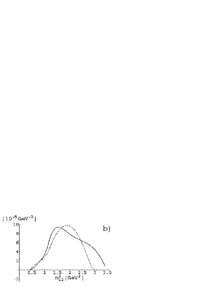
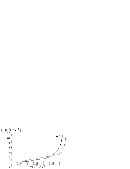
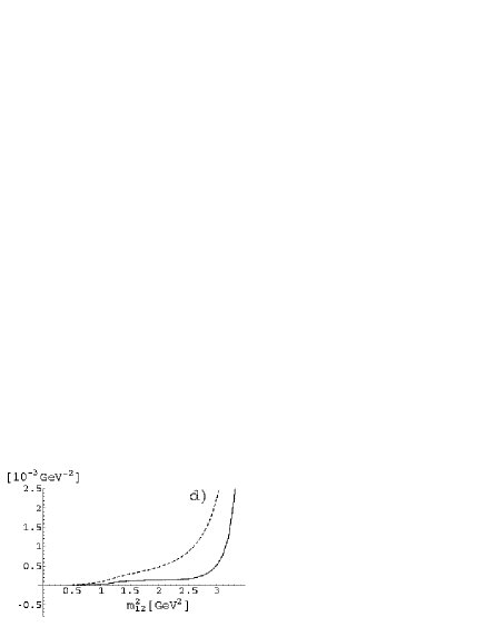
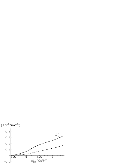
Figure 5: $\frac{1}{\Gamma_{total}}\frac{d\Gamma}{dm_{12}}$ for the decay $D^{+}\to\bar{K}^{0}\pi^{+}\gamma$ (left) and $D^{0}\to K^{-}\pi^{+}\gamma$ (right). Above: Direct parity - conserving (dashed line) and parity - violating (putting $F_{0}=0$) (full line) terms. Middle: $\frac{1}{\Gamma_{total}}\frac{d\Gamma}{dm_{12}}$ with $\Gamma$ containing the full decay amplitudes, for model (dashed line) and model+exp. (full line). For the latter, maximal $F_{0}$, $F_{1}$ interference is exhibited. Below: $\frac{1}{\Gamma_{total}}\frac{d\Gamma}{dm_{12}}$ with $\Gamma$ for the radiative decay calculated from model+exp. (full - line) compared to pure bremsstrahlung emission (dashed - line).

If we disregard the contribution of vector mesons, the rates are reduced to $BR(D^{+}\to\bar{K}^{0}\pi^{+}\gamma)_{PC}^{noVM}=$ $3.0\times 10^{-6}$ and $BR(D^{0}\to K^{-}\pi^{+}\gamma)_{PC}^{noVM}=$ $6.6\times 10^{-7}$. The decrease is sharper for the $D^{0}$ decay, since in this case the light vector mesons gave the dominant contribution to the rate, this is not the case for $D^{+}$ where such a contribution is doubly Cabibbo suppressed. The differential distribution for these transitions, as a function of $m_{12}^{2}=(P-k)^{2}$, is given as the dashed line distribution in Fig. 5a, 5b, for these two decays. The distribution is mainly symmetrical, with the peak occuring at $k\simeq 400$ ${\rm MeV}$. Thus, this is the region in which the effect of the direct transition has best chance for detection.

Turning to the parity - violating transitions we start with the procedure whereby we enforce the Low theorem by using Eq. (25). Here we face the question of unknown phase between $F_{0}$ and $F_{1}$. We give therfore the results in terms of a range, limited by minimal and maximal interference between $F_{0}$ and $F_{1}$.

Thus, we get for the branching ratios of the electric transitions, with $|F_{0}|$ determined experimentally,

$$BR(D^{+}\to\bar{K}^{0}\pi^{+}\gamma)_{PV,ex}^{k>50MeV}=(3.6-3.8)\times 10^{-4},$$ (34)

$$BR(D^{+}\to\bar{K}^{0}\pi^{+}\gamma)_{PV,ex}^{k>100MeV}=(2.3-2.5)\times 10^{-4}.$$ (35)

For the $D^{0}$ radiative decay we get

$$BR(D^{0}\to K^{-}\pi^{+}\gamma)_{PV,ex}^{k>50MeV}=(5.0-15)\times 10^{-4},$$ (36)

$$BR(D^{0}\to K^{-}\pi^{+}\gamma)_{PV,ex}^{k>100MeV}=(2.6-11)\times 10^{-4}.$$ (37)

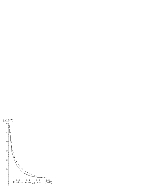
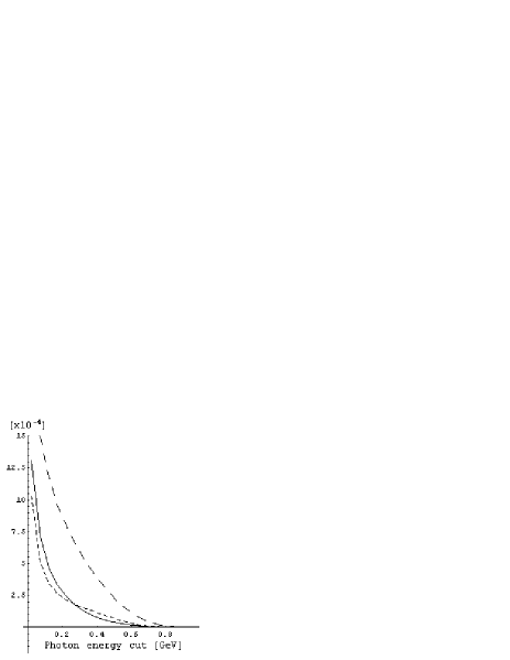
Figure 6: Branching ratio of radiative decays. Left: Decay $D^{+}\to\bar{K}^{0}\pi^{+}\gamma$ Right: Decay $D^{0}\to K^{-}\pi^{+}\gamma$ Full line: Bremsstrahlung only. Long dashed line: all contributions included and pozitive $F_{0}$, $F_{1}$ interference; short dashed line: negative interference

The uncertainty in the $F_{0}/F_{1}$ phase is less of a problem in $D^{+}\to\bar{K}^{0}\pi^{+}\gamma$ than in $D^{0}\to K^{-}\pi^{+}\gamma$. If we take the bremsstrahlung amplitude alone as determined from the knowledge of $|F_{0}|$, disregarding the direct electric $F_{1}$ term, the above numbers are replaced by $3.6\times 10^{-4}$ and $2.3\times 10^{-4}$ for $D^{+}$ decay and $8.6\times 10^{-4}$ and $5.5\times 10^{-4}$ for the $D^{0}$ decay. In Fig. 6 we also show the dependence of the branching ratio of the bremsstrahlung amplitude on the lower energy bound, for both decays. The contribution of the direct parity violating term (putting $F_{0}=0$ ), is $BR(D^{+}\to\bar{K}^{0}\pi^{+}\gamma)_{dir,PV}$ $=1.0\times 10^{-5}$ and $BR(D^{0}\to K^{-}\pi^{+}\gamma)_{dir,PV}$ $=1.64\times 10^{-4}$.

We checked also for the PV-transition the effect of the vector mesons. Using the Lagrangian of Refs. [22, 23] we found that in the PV-transition the effect of vector mesons is rather negligible; there is practically no change in (34), (35) and only a a narrowing of the range in (36) and (37), to bring it essentially to the values of pure bremsstrahlung we indicated after Eq. (37).

We have calculated the decay rates also by using our model, for the whole radiative amplitudes i.e. using all graphs of Figs. 1-4. Comparing these results with those of Eq. (34) - (37) gives an indication of the possible uncertainty of our model. We obtain

$$BR(D^{+}\to\bar{K}^{0}\pi^{+}\gamma)_{PV,model}^{k>50MeV}=3.0\times 10^{-4},$$ (38)

$$BR(D^{+}\to\bar{K}^{0}\pi^{+}\gamma)_{PV,model}^{k>100MeV}=2.5\times 10^{-4}.$$ (39)

For the $D^{0}$ radiative decay we get

$$BR(D^{0}\to K^{-}\pi^{+}\gamma)_{PV,model}^{k>50MeV}=2.3\times 10^{-3},$$ (40)

$$BR(D^{0}\to K^{-}\pi^{+}\gamma)_{PV,model}^{k>100MeV}=1.5\times 10^{-3}.$$ (41)

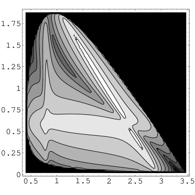
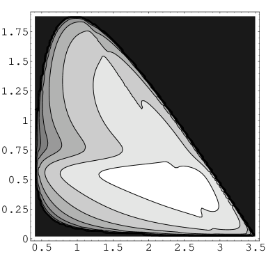
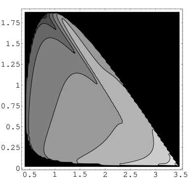
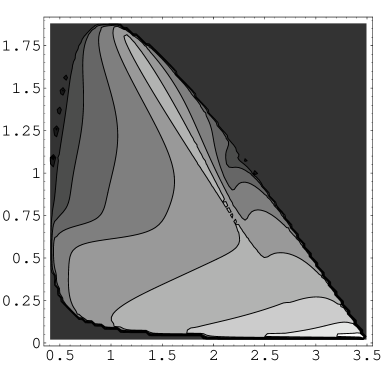
Figure 7: Dalitz plot of the parity conserving (above) and parity violating part (below) of the $D^{0}\to K^{-}\pi^{+}\gamma$ (left) and $D^{+}\to\bar{K}^{0}\pi^{+}\gamma$ decay (right). With gray levels on contour plot (left) and on z axis on the 3D plot (right) we present $\frac{2}{G_{F}}d\Gamma/(dm_{12}dm_{23})$ in the logarithmic scale. Invariant mass $m_{12}=\sqrt{(P-k)^{2}}$ is plotted on the x axis and $m_{23}=\sqrt{(P-p)^{2}}$ on the y axis of contour plot. The x and y axes of the 3D plot are labeled.

In Fig. 5c, 5d, we compare the rate of the decays $d\Gamma=d\Gamma_{PC}+d\Gamma_{PV}$ for the two alternative calculations concerning the PV part. In Fig. 5e, 5f we compare the rate of decay, $d\Gamma=d\Gamma_{PC}+d\Gamma_{PV}$ calculated from (S0.Ex7) to the bremsstrahlung rate, to emphasize the feasibilty of detecting the direct emission. Finally, in Fig. 7 we present Dalitz plots for these decays.

IV. DISCUSSION AND SUMMARY

The calculation we presented is the first attempt to formulate a theoretical framework for decays of type $D\to K\pi\gamma$, with nonresonant $K\pi$. The calculational framework is the strong Lagrangian (12)-(15) used in the tree approximation, and factorization for the weak matrix elements. In the present article we treat the Cabibbo allowed decays and among these, only channels which have both inner bremsstrahlung and direct radiation components, $D^{+}\to\bar{K}^{0}\pi^{+}\gamma$ and $D^{0}\to K^{-}\pi^{+}\gamma$, i.e. those which are the most likely ones for early detection. There is a third channel in this class, $D^{0}\to\bar{K}^{0}\pi^{0}\gamma$, which has only a direct component in the radiative decay and will be discussed separately.

Our results show that the relative expected strengths of the direct and bremsstrahlung components are of a magnitude which would permit the experimental determination of both, in next generation of experiments. This is important, since the direct amplitude provides information on the decay mechanism. In the radiative decay of $D^{+}$, the magnetic direct component amounts to about $6\%$ of the total rate (see Eqs. (33), (35)) and together with direct electric component which is of comparable magnitude (see Fig. 5a), dominate the decay spectrum in the region of high photon energies, say above $k\simeq 250$ ${\rm MeV}$ (see Fig. 5f). A similar situation occurs in the $D^{0}\to K^{-}\pi^{+}\gamma$ transition, where the direct radiative decay containing both electric and magnetic parts which are of nearly equal magnitude, amounts to over $30\%$ of the total radiative decay rate (see Eqs. (34) and (37)). The numbers we mentioned are for $k>50$ ${\rm MeV}$, but as we stressed the region of high photon momenta beyond $200$ ${\rm MeV}$ is where the direct transition even dominates.

The above large relative rates of direct/IB are somewhat similar to the occurences in $K_{2}^{0}\to\pi^{+}\pi^{-}\gamma$ and $K^{+}\to\pi^{+}\pi^{0}\gamma$, although in the D decays there is no apparant suppression of the original decays. This is most probably related to the mechanism of the decay provided by the heavy quark Lagrangian and the coupling constants involved, e.g. the rather large value of $|g|=0.59$ as recently determined.

We have checked the sensitivity of our results to various parameters we used. The uncertainty in the strong coupling $g=0.59\pm 0.07$, may change our results for direct branching ratios by at most $15\%$. On the other hand, the uncertainty in $\lambda$ and $\lambda^{\prime}$, and changing of sign of $\alpha_{1,2}$ is comparably negligible. As to the values of $f_{D}$, if we vary it by a reasonable amount we can induce changes in the direct amplitudes by a few tens of percent. Althogeter, we feel that with the assumed calculational framework, the calculated direct amplitudes do not have uncertainties of more than $50\%$. Another feature which we neglect is the role of possible axial and scalar resonances, where the experimental situation is rather unsettled.

As we explained in the text, the results (35) -(38) are obtained by using the experimental $D\to K\pi$ amplitudes to calculate the inner bremsstrahlung. If we use the model for doing it, we get the result exhibited in (39)- (42), which do not differ from (35), (36), i.e. the $D^{+}\to\bar{K}^{0}\pi^{+}\gamma$ decay, but are larger by a factor of about 2 in the amplitude in the case of $D^{0}\to K^{-}\pi^{+}\gamma$ decay. This is apparently related to the known difficulty of calculating the $D^{0}\to K^{-}\pi^{+}$ amplitude in the factorization approximation; therefore, we consider the results given in (37), (38) to be on a safer ground.

If we disregard the contribution of vector mesons to the direct part of the radiative decays, the parity-conserving part of the amplitude is considerably decreased, by one order of magnitude in the rate in $D^{+}\to\bar{K}^{0}\pi^{+}\gamma$ decay and by two orders of magnitude in $D^{0}\to K^{-}\pi^{+}\gamma$. On the other hand, their contribution is not felt in a significant way in in the parity - violating part of the amplitudes. In any case, the detection of the direct part of these decays at the predicted rates, will constitute a proof of the important role of the light vector mesons. The contribution of the vector mesons in the crossed channels is evident in the Dalitz plots of Fig.7. We point out that the contribution of the vector mesons in $F_{1}$, as evidenced from the relevant graphs, is wholy determined by the $\lambda$, $\lambda^{\prime}$ couplings.

Figs. 5a, 5b give the expected spectra for the direct component, which would be detectable in the region of high photon energioes. For the $D^{+}$ decay, the direct electric and magnetic transitions are of comparable strength. This prediction of the model should be testable, as it shiffts the peak of the spectrum to $E_{\gamma}=480$ ${\rm MeV}$, while if the magnetic transition is dominant it should peak $E_{\gamma}=400$ ${\rm MeV}$. In the $D^{0}\to K^{-}\pi^{+}\gamma$ decay the magnetic and electric components are likewise of nearly equal size, again testable in the spectrum. It is worthwhile to point out that the relative values of the parity - conserving amplitudes is rather large $|A(D^{0}\to K^{-}\pi^{+}\gamma)|^{2}/|A(D^{+}\to\bar{K}^{0}\pi^{+}\gamma)|^{2}$ $\simeq 7$. The main reason for it are certain contributions (like $D_{1,1}^{0}$), which appear in $D^{0}$ decay but are doubly Cabibbo forbidded in the $D^{+}$ decay. Also, as we pointed out, the $\Delta I=1/2$ amplitude is larger than the $\Delta I=3/2$ one in the $D\to K\pi$ channels.

Finally, we wish to emphasize a most interesting implication of our calculation. When one compares the results obtained here for the radiative decays to nonresonant $K\pi$, with those previously obtained for the $D\to K^{*}\gamma$ [4,6,7,16], it emerges that the nonresonant channel is the more frequent one. Thus, while one expects for $D^{+}\to K^{*+}\gamma$ a branching ratio (BR) of about $10^{-6}$ (this decay being doubly Cabibbo suppressed), the direct decay $D^{+}\to\bar{K}^{0}\pi^{+}\gamma$ is expected to have a BR of $\simeq 3\times 10^{-5}$ in our model. To this one should add the IB component, which brings its BR to about $4\times 10^{-4}$ for $k>50$ ${\rm MeV}$. The radiative decay $D^{0}\to\bar{K}^{*0}\gamma$ is expected with BR of $0.5\times 10^{-4}$. The nonresonant direct $D^{0}\to K^{-}\pi^{+}\gamma$ decay we investigated here, has a BR of $\simeq 3\times 10^{-4}$ and including the IB component will occur with a rate $8\times 10^{-4}$ for $k>50$ ${\rm MeV}$. The experimental verification of this systematics will provide a check for the suitabilty of the theoretical methods employed. We should remark,however, at this point that we did not address the possibility of the decays $D\to R+\gamma$ , where R is a higher $K\pi$ or $K\pi\pi$ resonance. To our knowledge, there is no calculation available on this topic. Our expectation is that such modes are at most comparable in strength to the $D\to\bar{K}^{*}\gamma$ decay; preliminary data from BELLE [42] indicate that this is the case in B decays.

There is another feature of interest which we mention. Since there is interference between the direct electric and the bremsstrahlung component of the amplitude, these decays can also be used to test CP - violating effects in the amplitudes.

We conclude by expressing the hope that the interesting features which these decays provide and were analyzed in this paper, will bring to an experimental search in the near future.

ACKNOWLEDGMENTS

We thank our colleagues Y. Rosen, S. Tarem and P. Križan for stimulating discussions on experimental aspects of this investigation.

The research of S.F. and A.P. was supported in part by the Ministry of Education, Science and Sport of the Republic of Slovenia. The research of P.S. was supported in part by Fund for Promotion of Research at the Technion.

APPENDIX A: THE DECAY AMPLITUDES FOR $D^{+}\to\bar{K}^{0}\pi^{+}\gamma$

Here we give the expressions for the sum of amplitudes in each row presented in Fig 1. The contributions which arise due to $O_{1}$ operator are:

$$A^{+}_{1}=-ie\frac{f_{D}f_{\pi}}{f_{K}}\frac{(v\cdot q+v\cdot k)p\cdot k}{v\cdot k}\;,$$

$$A^{+}_{2}=-ie\sqrt{\frac{M_{s}}{M}}\frac{f_{Ds}f_{\pi}}{f_{K}}g\frac{p\cdot q-(v\cdot q)(v\cdot p)+v\cdot k(M-v\cdot p)}{v\cdot p+\Delta}\frac{p\cdot k}{v\cdot k}\;,$$

$$A^{+}_{3}=ieg\sqrt{\frac{M_{s}}{M}}\frac{f_{Ds}f_{\pi}}{f_{K}}\frac{(v\cdot k)(q\cdot k)(p\cdot k)}{v\cdot k+v\cdot p+\Delta}$$

$$\left(\frac{-1}{v\cdot k+\Delta}\left(2\lambda^{{}^{\prime}}-\frac{\sqrt{2}}{2}\lambda g_{v}\left(\frac{q_{\omega}}{3m_{\omega}^{2}}-\frac{q_{\rho}}{m_{\rho}^{2}}\right)\right)+\frac{1}{v\cdot p+\Delta}\left(2\lambda^{{}^{\prime}}-\frac{\sqrt{2}}{3}\lambda g_{v}\frac{q_{\phi}}{m_{\phi}^{2}}\right)\right)\;,$$

$$A^{+}_{4}=i\sqrt{2}f_{Ds}f_{\pi}g_{\bar{K}^{0*}\bar{K}^{0}\gamma}g_{v}\lambda e\sqrt{M_{s}M}\frac{(v\cdot k)(q\cdot k)^{2}}{(v\cdot(p+k)+\Delta)((p+k)^{2}-m_{K^{*}}^{2}+i\Gamma_{K^{*}}m_{K^{*}})}\;.$$

The contributions coming from $O_{2}$ operator are:

$$C^{+}_{1}=-ie\frac{f_{D}f_{K}}{f_{\pi}}\frac{(v\cdot p)(p\cdot k)}{v\cdot k}\;^{\prime}$$

$$C^{+}_{2}=ie\frac{f_{D}f_{K}}{f_{\pi}}g\frac{p\cdot q-(v\cdot p)(v\cdot q)+v\cdot k(M-v\cdot p)}{v\cdot q+v\cdot k+\Delta}\frac{p\cdot k}{v\cdot k}\;,$$

$$C^{+}_{3}=-ieg\frac{f_{D}f_{K}}{f_{\pi}}\frac{(v\cdot k)(q\cdot k)}{p\cdot k(v\cdot k+v\cdot q+\Delta)}$$

$$\left(\frac{-1}{v\cdot k+\Delta}\left(2\lambda^{{}^{\prime}}-\frac{\sqrt{2}}{2}\lambda g_{v}\left(\frac{q_{\omega}}{3m_{\omega}^{2}}-\frac{q_{\rho}}{m_{\rho}^{2}}\right)\right)-\frac{1}{v\cdot q+\Delta}\frac{\sqrt{2}}{2}\lambda g_{v}\left(\frac{q_{\omega}}{3m_{\omega}^{2}}+\frac{q_{\rho}}{m_{\rho}^{2}}\right)\right)\;,$$

$$C^{+}_{4}=-i\sqrt{2}f_{D}f_{K}g_{\rho\pi\gamma}g_{v}\lambda eM\frac{(v\cdot k)(p\cdot k)^{2}}{(v\cdot(q+k)+\Delta)((q+k)^{2}-m_{\rho}^{2}+i\Gamma_{\rho}m_{\rho})}\;.$$

Next we give the expressions for the sum of amplitudes in each row presented in Fig 2. The contributions arising from the $O_{1}$ operator:

$$B^{+}_{1}=2eM\frac{f_{D}f_{\pi}}{f_{K}}\lambda^{,}\left(\frac{1}{v\cdot k+\Delta}+g\frac{f_{Ds}\sqrt{M_{s}}}{f_{D}\sqrt{M}}\frac{v\cdot q}{v\cdot p+v\cdot k}\left(\frac{1}{v\cdot k+\Delta}+\frac{1}{v\cdot p+\Delta}\right)\right)\;,$$

$$B^{+}_{2}=-\sqrt{2M}eg_{v}g_{\bar{K}^{0*}\bar{K}^{0}\gamma}f_{\pi}\frac{\alpha_{1}M-\alpha_{2}v\cdot q}{(p+k)^{2}-m_{K*}^{2}-i\Gamma_{K^{*}}m_{K^{*}}}$$

$$+eg_{\rho\pi\gamma}g_{\rho}\frac{f_{D}}{f_{K}}\sqrt{M}\frac{\sqrt{M}+\frac{f_{Ds}}{f_{D}}\sqrt{M_{s}}g\frac{M-v\cdot p}{v\cdot p+\Delta}}{(k+q)^{2}-m\rho^{2}+i\Gamma_{\rho}m_{\rho}}\;,$$

$$B^{+}_{3}=-\frac{1}{\sqrt{2}}e\frac{f_{\pi}}{f_{K}}\lambda g_{v}\left(\frac{q_{\omega}}{3m_{\omega}^{2}}-\frac{q_{\rho}}{m_{\rho}^{2}}\right)\frac{1}{(v\cdot k+\Delta)}\left(Mf_{D}+\sqrt{MM_{s}}f_{Ds}\frac{v\cdot q}{v\cdot k+v\cdot p}\right)$$

$$+\frac{\sqrt{2}}{3}\sqrt{MM_{s}}e\frac{f_{Ds}f_{\pi}}{f_{K}}g\lambda g_{v}\frac{q_{\phi}}{m_{\phi}^{2}}\frac{v\cdot q}{(v\cdot p+\Delta)(v\cdot k+v\cdot p)}\;.$$

The operator $O_{2}$ gives the following contributions:

$$D^{+}_{1}=-2eM\frac{f_{D}f_{K}}{f_{\pi}}\lambda^{,}\left(\frac{1}{v\cdot k+\Delta}+g\frac{v\cdot p}{(v\cdot q+v\cdot k)(v\cdot k+\Delta)}\right)\;,$$

$$D^{+}_{2}=\sqrt{2M}eg_{v}g_{\rho\pi\gamma}f_{K}\frac{\alpha_{1}M-\alpha_{2}v\cdot p}{(q+k)^{2}-m_{\rho}^{2}+i\Gamma_{\rho}m_{\rho}}$$

$$-eg_{\bar{K}^{0*}\bar{K}^{0}\gamma}g_{K^{*}}\frac{f_{D}}{f_{\pi}}M\frac{1+g\frac{M-v\cdot q}{v\cdot q+\Delta}}{(v\cdot q)((k+p)^{2}-m_{K^{*}}^{2}+i\Gamma_{K^{*}}m_{K^{*}})}\;,$$

$$D^{+}_{3}=\frac{1}{\sqrt{2}}Me\frac{f_{D}f_{K}}{f_{\pi}}\lambda g_{v}\left(\frac{q_{\omega}}{3m_{\omega}^{2}}-\frac{q_{\rho}}{m_{\rho}^{2}}\right)\frac{1}{(v\cdot k+\Delta)}\left(1+g\frac{v\cdot p}{v\cdot k+v\cdot q}\right)$$

$$+\frac{1}{\sqrt{2}}Me\frac{f_{D}f_{K}}{f_{\pi}}g\lambda g_{v}\frac{v\cdot p}{(v\cdot q+\Delta)(v\cdot k+v\cdot q)}\left(\frac{q_{\omega}}{3m_{\omega}^{2}}+\frac{q_{\rho}}{m_{\rho}^{2}}\right)\;.$$

APPENDIX B: THE DECAY AMPLITUDES FOR $D^{0}\to K^{-}\pi^{+}\gamma$

The expressions for the sum of amplitudes (the $O_{1}$ operator) in each row exhibited in Fig 3. are:

$$A^{0}_{1}=-iMe\frac{f_{D}f_{\pi}}{f_{K}}(v\cdot q+v\cdot k)\;,$$

$$A^{0}_{2}=ie\sqrt{MM_{s}}\frac{f_{Ds}f_{\pi}}{f_{K}}g\left(\frac{p\cdot k(v\cdot p-M)}{M(v\cdot p+\Delta)}-\frac{p\cdot k(p\cdot q-(v\cdot p)(v\cdot q))}{M(v\cdot p+\Delta)(v\cdot p+v\cdot k+\Delta)}\right.$$

$$\qquad\left.+\frac{Mq\cdot k-Mp\cdot q+M(v\cdot q)(v\cdot p)-(v\cdot q)(q\cdot k)}{M(v\cdot p+v\cdot k+\Delta)}\right)\;,$$

$$A^{0}_{3}=ie\sqrt{M_{s}/M}\frac{f_{Ds}f_{\pi}}{f_{K}}g\frac{(v\cdot k)(p\cdot k)(q\cdot k)}{(v\cdot k+v\cdot p+\Delta)}\left(\frac{2\lambda^{{}^{\prime}}-\frac{\sqrt{2}}{3}\lambda g_{v}\frac{q_{\phi}}{m_{\phi}^{2}}}{(v\cdot p+\Delta)}+\frac{\frac{\sqrt{2}}{2}\lambda g_{v}\left(\frac{q_{\omega}}{3m_{\omega}^{2}}+\frac{q_{\rho}}{m_{\rho}^{2}}\right)}{v\cdot k+\Delta}\right)\;,$$

$$A^{0}_{4}=i\sqrt{2}f_{Ds}f_{\pi}g_{K^{*}K\gamma}g_{v}\lambda e\sqrt{M_{s}M}\frac{(v\cdot k)(q\cdot k)^{2}}{(v\cdot(p+k)+\Delta)((p+k)^{2}-m_{K^{*}}^{2}+i\Gamma_{K^{*}}m_{K^{*}})}\;.$$

The sum of amplitudes coming from operator $O_{2}$, shown in Fig. 3 as $C^{0}_{1}$, is vanishing.

Next we present the expressions for the sums of amplitudes in each row shown in Fig. 4. The results for the operator $O_{1}$ are:

$$B^{0}_{1}=e\sqrt{MM_{s}}\frac{f_{Ds}f_{\pi}}{f_{K}}\frac{g(v\cdot q)}{(v\cdot p+\Delta)(v\cdot k+v\cdot p)}\left(2\lambda^{{}^{\prime}}+\frac{\sqrt{2}}{3}\lambda g_{v}\frac{q_{\phi}}{m_{\phi}^{2}}\right)$$

$$+\frac{1}{\sqrt{2}}Me\frac{f_{\pi}}{f_{K}}\lambda g_{v}\frac{1}{(v\cdot k+\Delta)}\left(f_{D}\left(\frac{q_{\omega}}{3m_{\omega}^{2}}+\frac{q_{\rho}}{m_{\rho}^{2}}\right)+f_{Ds}\sqrt{\frac{M_{s}}{M}}\left(\frac{q_{\omega}}{3m_{\omega}^{2}}-\frac{q_{\rho}}{m_{\rho}^{2}}\right)\frac{gv\cdot q}{(v\cdot k+v\cdot p)}\right)\;,$$

$$B^{0}_{2}=-\sqrt{2M}eg_{v}g_{\bar{K}^{*}\bar{K}^{\gamma}}f_{\pi}\frac{\alpha_{1}M-\alpha_{2}v\cdot q}{(p+k)^{2}-m_{K*}^{2}+i\Gamma_{K^{*}}m_{K^{*}}}$$

$$+eg_{\rho\pi\gamma}g_{\rho}\frac{f_{D}}{f_{K}}\frac{M+\frac{f_{Ds}}{f_{D}}\sqrt{M_{s}M}g\frac{M-v\cdot p}{v\cdot p+\Delta}}{(k+q)^{2}-m_{\rho}^{2}+i\Gamma_{\rho}m_{\rho}}\;.$$

Finally, the sums of amplitudes in each row due to the operator $O_{2}$:

$$D^{0}_{1}=\frac{M}{\sqrt{2}}e\lambda g_{v}f_{D}\left(\frac{q_{\omega}}{3m_{\omega}^{2}}+\frac{q_{\rho}}{m_{\rho}^{2}}\right)\frac{1}{v\cdot k+\Delta}\left(1+\frac{m_{\bar{K}^{0}}^{2}}{(p+q)^{2}-m^{2}_{\bar{K}^{0}}}\right)\;,$$

$$D^{0}_{2}=Me\frac{f_{D}}{f_{\pi}}g_{K}g_{KK^{*}\gamma}\frac{1}{(p+k)^{2}-m^{2}_{K^{*}}+im_{K^{*}}\Gamma_{K^{*}}}+Me\frac{f_{D}}{f_{K}}g_{\rho}g_{\rho\pi\gamma}\frac{1}{(q+k)^{2}-m^{2}_{\rho}+im_{\rho}\Gamma_{\rho}}\;,$$

$$D^{0}_{3}=-\frac{e}{2}f_{D}f_{K}\frac{m^{2}_{K^{*}}}{g_{K^{*}}}\frac{M^{3}}{(M^{2}-m^{2}_{\bar{K}^{0}})}\left(\frac{g_{K^{*}K\gamma}}{(p+k)^{2}-m^{2}_{K^{*}}+im_{K^{*}}\Gamma_{K^{*}})}+\frac{g_{\rho\pi\gamma}}{(q+k)^{2}-m^{2}_{\rho}+im_{\rho}\Gamma_{\rho})}\right)\;.$$

Figure 1: Feynman diagrams contributing to the formfactor $F_{1}$ of the $D^{+}\to\bar{K}^{0}\pi^{+}\gamma$ decay. Diagrams denoted by $A^{+}_{i,j}$ ($C^{+}_{i,j}$) come from the operator $O_{1}$ ($O_{2}$). Sum of the contributions of each row is gauge invariant. In diagrams $A^{+}_{3,1}$, $A^{+}_{3,2}$, $C^{+}_{3,1}$ and $C^{+}_{3,2}$ the photon couples to the heavy mesons with strength $\lambda^{{}^{\prime}}$.

Figure 2: Feynman diagrams contributing to the formfactor $F_{2}$ of the $D^{+}\to\bar{K}^{0}\pi^{+}\gamma$ decay. Diagrams denoted by $B^{0}_{i,j}$ ($D^{0}_{i,j}$) come from the operator $O_{1}$ ($O_{2}$).

Figure 3: Feynman diagrams contributing to the formfactor $F_{1}$ of the $D^{0}\to K^{-}\pi^{+}\gamma$ decay. Diagrams denoted by $A^{+}_{i,j}$ ($C^{+}_{i,j}$) come from the operator $O_{1}$ ($O_{2}$). Sum of the contributions of each row is gauge invariant. In diagrams $A^{0}_{3,1}$ and $A^{0}_{3,2}$ the photon couples to the heavy mesons with strength $\lambda^{{}^{\prime}}$.

Figure 4: Feynman diagrams contributing to the formfactor $F_{2}$ of the $D^{0}\to K^{-}\pi^{+}\gamma$ decay. Diagrams denoted by $B^{+}_{i,j}$ ($D^{+}_{i,j}$) come from the operator $O_{1}$ ($O_{2}$).

References

[1] S. Fajfer, S. Prelovšek, P. Singer, and D. Wyler,
Phys. Lett. B 487, 81 (2000).
[2] G. Burdman, E. Golowich, J. L. Hewett, and S. Pakvasa,
hep-ph/0112235.
[3] S. Fajfer, S. Prelovšek, P. Singer, Phys. Rev. D
64, 114009 (2001).
[4] S. Prelovšek, PhD-thesis, hep-ph/0010106.
[5] D.M. Asner et al., CLEO Collaboration,
Phys. Rev D 58, 092001 (1998).
[6] S. Fajfer, S. Prelovšek, and P. Singer, Eur. Phys. J. C
6, 471 (1999);6, 751(E) (1999).
[7] R.F. Lebed, Phys. Rev. D 61, 033004 (2000).
[8] A. Freyberger et al., CLEO collaboration,
Phys. Rev. Lett. 76, 3065 (1996);
E. M. Aitala et al., E 791 Collaboration, Phys. Rev. Lett. 76,
364 (1996); Phys. Lett. B 462, 401 (1999);
D. A. Sanders, Mod. Phys. Lett. A 15, 1399 (2000).
[9] S. Fajfer, S. Prelovšek, P. Singer, Phys. Rev. D
58, 094038 (1998).
[10] E. M. Aitala et al., E 791 Collaboration,
Phys. Rev. Lett. 86,
3969 (2001); D. A. Sanders et al., E791 Collaboration,
hep-ph/0105028; D. J. Summers, Int. J. Mod. Phys.
A 16, Suppl. 1B, 536 (2001).
[11]
M. Moshe and P. Singer, Phys. Lett. B 51, 367 (1974);
G. Ecker, H. Neufeld, and A. Pich, Phys.
Lett. B 278, 337 (1992); G. D’Ambrosio and D.-N. Gao,
JHEP 0010, 043 (2000).
[12] J. Bijnens, G. Ecker, and A. Pich,
Phys. Lett. B 286, 341 (1992), H.Y. Cheng, Phys. Rev. D
49, 3771 (1992); Y.C.R. Lin and G. Valencia, Phys. Rev. D 37, 143
(1988).
[13]S. Fajfer, Z. Phys. C 45, 293 (1989).
[14] Q.H. Kim and X. Y. Pham, Phys. Rev. 61, 013008
(2000).
[15] G. Greub, T. Hurth, M. Misiak and D. Wyler, Phys. Lett.
B 382, 415 (1996).
[16] G. Burdman, E. Golowich, J. L. Hewett and S. Pakvasa,
Phys. Rev. D 52, 6383 (1995).
[17] B. Bajc, S. Fajfer, R. J. Oakes, and S. Prelovšek,
Phys. Rev. D 56,
7207 (1997).
[18] A. N. Kamal, A. B. Santra, T. Uppal and R. C. Verma,
Phys. Rev. D 53, 2506 (1996).
[19] M. Bauer, B. Stech and M. Wirbel, Z. Phys. C
34, 103 (1987);
M. Neubert , V. Rieckert, B. Stech and Q. P. Xu, in: Heavy
Flavours, eds.
A. J.Buras and M. Linder (World Scientific, Singapore, 1992)
p. 286; H. Y. Cheng, hep-ph/0202254.
[20] B. Bajc, S. Fajfer, and R. J. Oakes, Phys. Rev. D 53,
4957 (1996).
[21] M.B. Wise, Phys. Rev. D 45, R2188 (1992);
G. Burdman and J. F.
Donoghue, Phys. Lett. B 280, 287 (1992).
[22] T.M. Yan et al.,
Phys. Rev. D 46, 1148 (1992).
[23] R. Casalbuoni et al.,
Phys. Lett. B 299, 139 (1993); Phys. Rep. 281, 145
(1997).
[24] B. Bajc, S. Fajfer, and R. J. Oakes,
Phys. Rev. D 51, 2230 (1995).
[25]
Review of Particle Physics, D. E. Groom et al., Eur.
Phys. J. C 15, 1 (2000).
[26] J.L. Rosner, Phys. Rev. D 60, 074029 (1999);
M. Suzuki, Phys. Rev. D 60, 051501 (1999).
[27] S. Fajfer and P. Singer, Phys. Rev. D 56, 4302 (1997).
[28] M. Bando, T. Kugo, S. Uehara,
K. Yamawaki and T. Yanagida, Phys. Rev. Lett.
54, 1215 (1985);
M. Bando, T. Kugo, and K. Yamawaki,
Nucl. Phys. B 259, 493 (1985);
Phys. Rep. 164, 217 (1988).
[29] T. Fujiwara, T. Kugo, H. Terao, S. Vehara,
and K. Yamawaki, Prog. Th. Phys. 73, 926 (1985).
[30] G. Eilam, A. Ioannissian, R. R. Mendel, and P. Singer,
Phys. Rev. D 53, 3629 (1996).
[31] D. Guetta and P. Singer, Phys. Rev. D 61, 054014
(2000); P. Singer, Acta Phys. Polon. B 30, 3849 (1999).
[32] A. Anastassov et al., CLEO Collaboration, Phys. Rev. D 65, 032003 (2002).
[33] A. Bramon, A. Grau, and G. Pancheri, Phys. Lett. B 344,
240 (1995).
[34] P. Colangelo, F. De. Fazio, and G. Nardulli, Phys.
Lett. B 316, 555 (1993).
[35] P. Cho and H. Georgi, Phys. Lett. B. 296, 402 (1992).
[36] I. W. Stewart, Nucl. Phys. B 529, 62 (1998).
[37] S. Fajfer, P. Singer, and J. Zupan, Phys. Rev. D
64, 074008 (2001).
[38] J. D. Richman and P. R. Burchat, Rev. Mod. Phys. 67,
893 (1995).
[39] P. Singer, Phys. Rev. D 130, 2441 (1963);
161, 1694(E) (1967); M.
Sapir and P. Singer, Phys. Rev. 163, 1756 (1967).
[40] F. Low, Phys. Rev. 110, 974 (1958); H. Chew,
Phys. Rev. 123, 377 (1961).
[41] C. T. Sachrajda, Talk given at Lepton Photon conference
in Rome, July 2001, hep-ph/0110304.
[42] BELLE-CONF-0109.