Oscillation damping of chiral string loops

Abstract

Chiral cosmic string loop tends to the stationary (vorton) configuration due to the energy loss into the gravitational and electromagnetic radiation. We describe the asymptotic behaviour of near stationary chiral loops and their fading to vortons. General limits on the gravitational and electromagnetic energy losses by near stationary chiral loops are found. For these loops we estimate the oscillation damping time. We present solvable examples of gravitational radiation energy loss by some chiral loop configurations. The analytical dependence of string energy with time is found in the case of the chiral ring with small amplitude radial oscillations.

I Introduction

Cosmic strings are one-dimensional topological defects which may have formed during phase transition in the early universe Kibble1 ; Zel'dovich1 ; Vilenkin1 . Witten Witten1 has shown that strings could be superconducting in certain particle physics models. The presence of current in a string leads to the principal specific feature: the superconducting string loop may form a stable stationary configuration Davis1 ; Haws1 ; Haws2 . Cosmic strings lose their energy on gravitational and electromagnetic radiation (if string is superconducting). As a result, the “ordinary” not extremely long cosmic strings without the current evaporate completely during the cosmological time. On the contrary the superconducting string loops could survive due to the presence of conserved “charge” and tend to the stable configuration which is named the chiral vorton Davis1 .

Numerous works were devoted to calculations of the gravitational and electromagnetic radiation by cosmic strings (see reviews and references in Vilenkin2 ; Kibble2 ). Unfortunately the general problem of the motion of a superconducting cosmic string coupled to the electromagnetic field is not solved analytically. The using of Nambu-Goto equations of string motion in general case results in the singular cusp formation and the divergence of the electromagnetic power radiated by the string. Nevertheless equations of motion can be solved precisely Carter1 ; Davis2 ; Vilenkin3 if (i) the gauge field influence on the string motion is negligible, e.g. when the superconducting current is neutral, and (ii) the string current $J^{a}$ is chiral, i. e. $J^{a}J_{a}=0$, where $J^{a}$ is a two-dimensional current on the string world surface. It turns out that electromagnetic power radiated by the cusp of chiral cosmic strings is finite Blanco .

Self-consistent calculations of string evolution with time is complicated by the influence of the radiation back reaction on the string motion (see some approaches to numerical calculations of back reaction in Quashnock ). In this work we consider the electromagnetic and gravitational radiation by chiral strings loops which are close to the stationary vorton state (when amplitude of loop oscillations is very small). In this case it is physically justified the supposition that all string oscillations are faded out. We determine the upper bounds on gravitational and electromagnetic radiation of near stationary chiral loops when oscillations are small in amplitude. For some simple configurations of the string loops we calculate both types of radiation. We also find the analytical law for behavior in time of the string loop energy and current basing on the symmetries of the problem in the case when the final vorton configuration is the chiral ring and oscillations are radial. For some other less symmetric examples of loops we estimate the damping time of small amplitude oscillations. It turns out that in all considered examples the oscillation damping time of chiral strings due to gravitational radiation is order of magnitude longer than the known lifetime estimations for the “ordinary” cosmic strings without the current.

The paper is organized in the following order. Section II describes the general properties of the motion of chiral string loop in flat space-time. In Section III we consider the gravitational and electromagnetic radiation of the chiral string loops. The radiation power of the near stationary chiral loop with small amplitude oscillations is determined and the corresponding upper bounds for gravitational and electromagnetic radiation are found. Some solvable examples of near stationary chiral strings including radially oscillating ring are presented in Section IV. In Section V the damping time of weakly oscillating chiral loops is estimated and the exact time evolution law for radially oscillating chiral ring is found. Section VI briefly summarizes some features of the oscillation damping of chiral loops.

II Chiral string motion

We remind here the known basic properties of chiral string motion in flat space-time required for the following calculations. The moving string sweeps a two-dimensional world-sheet in the Minkowski space-time. The corresponding space-time points on this world-sheet $x^{\mu}=x^{\mu}(\sigma^{a})$, where indices $a=0,1$, and $\sigma^{0}$ and $\sigma^{1}$ are coordinates on a two-dimensional world-sheet. If the back reaction of electromagnetic and gravitational radiation is negligible, then equations of motion of the string with a current is given by Witten1 ; Vilenkin4

$$\partial_{a}\left[\sqrt{-\gamma}\left(\mu\gamma^{ab}+\theta^{ab}\right)x^{\nu}_{,b}\right]=0,$$

$$\partial_{a}\left(\sqrt{-\gamma}\gamma^{ab}\phi_{,b}\right)=0,$$ (1)

where $\gamma_{ab}=\eta_{ab}x^{\mu}_{,a}x^{\nu}_{,b}$ is the induced metric on a two-dimensional world-sheet, $\mu$ is the energy of a string per unit length, $\phi$ is the auxiliary scalar field and $\theta^{ab}$ is the energy-momentum tensor of the charge carriers

$$\theta^{ab}=\gamma^{ac}\gamma^{bd}\phi_{,c}\phi_{,d}-\frac{1}{2}\gamma^{ab}\gamma^{cd}\phi_{,c}\phi_{,d}\,.$$ (2)

The conserved current on a two-dimensional world-sheet is written in terms of the scalar field

$$J^{a}=\frac{q}{\sqrt{-\gamma}}\epsilon^{ab}\phi_{,b}\,,$$ (3)

where $q$ is the coupling constant of the fields in the string. The four-dimensional current is expressed through (3) as Vilenkin4

$$j^{\mu}(x)=\int d^{2}\sigma\sqrt{-\gamma}J^{a}x^{\mu}_{,a}\delta^{(4)}(x-x(\sigma)).$$ (4)

If this current is chiral, i. e.

$$J^{a}J_{a}=0,$$ (5)

then equations of motion (II) can be solved analytically Carter1 ; Davis1 ; Vilenkin3 . This solution for the chiral string with an invariant length $L$ is

$$x^{0}=t,\quad\mathbf{x}(t,\sigma)=\frac{L}{4\pi}\left[\mathbf{a}(\xi)+\mathbf{b}(\eta)\right],$$ (6)

where $\mathbf{a}(\xi)$ and $\mathbf{b}(\eta)$ are the vector functions of $\xi=(2\pi/L)(\sigma-t)$ and $\eta=(2\pi/L)(\sigma+t)$ obeying the constraints:

$${\mathbf{a}^{\prime}}^{2}=1,\quad{\mathbf{b}^{\prime}}^{2}\leq 1$$ (7)

For closed strings (with identified ends) the vector functions $\mathbf{a}(\xi)$ and $\mathbf{b}(\eta)$ define loops which are called $a$- and $b$- loops. The corresponding solution for scalar field is

$$\phi(\sigma,t)=\frac{L}{2\pi}F(\eta),$$ (8)

where $F(\eta)$ is an arbitrary function. It is useful to define ${\mathbf{b}^{\prime}}^{2}\equiv k^{2}(\eta)$. Then new function $k(\eta)$ is expressed through $F(\eta)$ in the following way:

$$k^{2}(\eta)=1-\frac{4F^{\prime 2}(\eta)}{\mu}.$$ (9)

At $k=0$ the chiral string becomes vorton.

The energy-momentum tensor of the string in this gauge

$$T^{\mu\nu}=\mu\int d\sigma\left(\dot{x}^{\mu}\dot{x}^{\nu}-x^{\prime\mu}x^{\prime\nu}\right)\delta^{(3)}\left(\mathbf{x}-\mathbf{x}(\sigma,t)\right),$$ (10)

and correspondingly the string total energy

$$E=\mu\int d\sigma,$$ (11)

with $\sigma$ to be the measure of the string total energy. The four-dimensional current (4) can be written as

$$j^{\mu}(\mathbf{x},t)=q\int d\sigma\phi^{\prime}(x^{\prime\mu}-\dot{x}^{\mu})\delta^{(3)}\left(\mathbf{x}-\mathbf{x}(\sigma,t)\right),$$ (12)

with the total charge for the closed string loop

$$q_{\rm tot}=\frac{q\sqrt{\mu}}{2}\int d\sigma\sqrt{1-k^{2}}.$$ (13)

III Chiral string radiation

III.1 Gravitational radiation

In the case of the periodic physical systems with period $T$ for the energy-momentum tensor $T_{\mu\nu}$ we will have $T^{\mu\nu}(\mathbf{x},t)=T^{\mu\nu}(\mathbf{x},t+T)$. Fourier series for $T_{\mu\nu}$ is

$$T^{\mu\nu}(\mathbf{x},t) = \sum_{l=1}^{\infty}e^{-i\omega_{l}t}T^{\mu\nu}(\omega_{l},\mathbf{x})+{\rm c.c},$$ (14)

where  ${\rm c.c}$  denotes the complex conjugation of the preceding expression, $\omega_{l}=2\pi l/T$ is the frequency and

$$T^{\mu\nu}(\omega_{l},\mathbf{x}) = \frac{1}{T}\int_{0}^{T}dte^{i\omega_{l}t}T^{\mu\nu}(\mathbf{x},t).$$ (15)

For $T^{\mu\nu}(\omega_{l},\mathbf{x})$ we have Fourier transform

$$\hat{T}^{\mu\nu}(\omega_{l},\mathbf{n}) = \int d^{3}xT^{\mu\nu}(\omega_{l},\mathbf{x})e^{-i\omega_{l}\mathbf{n}\mathbf{x}}$$ (16)

where $\mathbf{n}=\mathbf{x}/|\mathbf{x}|$.

The corresponding gravitational power, radiated per unit solid angle $d\Omega$ by periodic system is given by Weinberg

$$\frac{d\dot{E}^{\rm gr}}{d\Omega}=\sum_{l=1}^{\infty}\frac{d\dot{E}^{\rm gr}({\omega}_{l})}{d\Omega},$$ (17)

where

$$\frac{d\dot{E}^{\rm gr}({\omega_{l}})}{d\Omega}=\frac{G\omega^{2}_{l}}{\pi}P_{ij}P_{lm}[\hat{T}^{*}_{il}\hat{T}_{jm}-\frac{1}{2}\hat{T}^{*}_{ij}\hat{T}_{lm}].$$ (18)

Here $P_{ij}=\delta_{ij}-n_{i}n_{j}$ is the projection operator to the plane perpendicular to vector $\mathbf{n}$. It is possible to simplify the equation (18) further if rewrite it in the ‘corotating’ basis $(\mathbf{e}^{\prime}_{1},\mathbf{e}^{\prime}_{2},\mathbf{e}^{\prime}_{3})=(\mathbf{n},\mathbf{v},\mathbf{w})$, where $\mathbf{v}$ and $\mathbf{w}$ are the arbitrary unit vectors, perpendicular each other and to vector $\mathbf{n}$. In this corotating basis (18) transforms to Durrer

$$\frac{d\dot{E}^{\rm gr}({\omega_{l}})}{d\Omega}=\frac{G{\omega}^{2}_{l}}{\pi}[{\tau}^{*}_{pq}{\tau}_{pq}-\frac{1}{2}{\tau}^{*}_{qq}{\tau}_{pp}].$$ (19)

where $\tau_{pq}$ are correspondingly the Fourier-transforms of an energy-momentum tensor in the corotating basis. Only indexes $p,q$ with values $2$ and $3$ appear in the equation (19). The Fourier-transforms $\tau_{pq}$ can be expressed in the following way Durrer

$${\tau}_{pq}(\omega_{l},\mathbf{n})=-\frac{L\mu}{2}[I_{p}(l)Y_{q}(l)+Y_{p}(l)I_{q}(l)],$$ (20)

where functions $I_{p}(l)$ and $Y_{q}(l)$ are determined through ”fundamental integrals”

$$I_{2}(l) \equiv I_{l}(\mathbf{n},\mathbf{v}),\quad I_{3}(l)\equiv I_{l}(\mathbf{n},\mathbf{w}),$$

$$Y_{2}(l) \equiv Y_{l}(\mathbf{n},\mathbf{v}),\quad Y_{3}(l)\equiv Y_{l}(\mathbf{n},\mathbf{w}).$$ (21)

with

$$I_{l}(\mathbf{n},\mathbf{z}) \equiv \frac{1}{2\pi}\int_{0}^{2\pi}d\xi e^{-il(\xi+\mathbf{n}\mathbf{a}(\xi))}\mathbf{a}^{\prime}(\xi)\mathbf{z},$$ (22)

$$Y_{l}(\mathbf{n},\mathbf{z}) \equiv \frac{1}{2\pi}\int_{0}^{2\pi}d\eta e^{il(\eta-\mathbf{n}\mathbf{b}(\eta))}\mathbf{b}^{\prime}(\eta)\mathbf{z}.$$ (23)

Using functions (22) and (23) we rewrite the gravitational power (19) radiated per unit solid angle at frequency $\omega_{l}=4\pi l/L$ in the final form

$$\frac{d\dot{E}^{\rm gr}_{l}}{d\Omega} = 16\pi l^{2}G\mu^{2}\left\{\left|I_{2}(l)Y_{2}(l)\right|^{2}+\left|I_{3}(l)Y_{3}(l)\right|^{2}\right.$$

$$+\frac{1}{2}\left|I_{2}(l)Y_{3}(l)+I_{3}(l)Y_{2}(l)\right|^{2}$$

$$-\left.\frac{1}{2}\left|I_{2}(l)Y_{2}(l)+I_{3}(l)Y_{3}(l)\right|^{2}\right\}.$$

III.2 Electromagnetic radiation

We will consider the electromagnetic radiation of chiral strings close to the stationary configuration, i. e. when the current is near to its maximum value. For the opposite limiting case of electromagnetic radiating by the strings with a weak electromagnetic current see Blanco ; Berezinsky .

Similar to the case of the gravitational radiation, the electromagnetic power emitted per solid angle $d\Omega$ is expanded in Fourier series:

$$\frac{d\dot{E}^{\rm em}}{d\Omega}=\sum_{l=1}^{\infty}\frac{d\dot{E}^{\rm em}({\omega}_{l})}{d\Omega}.$$ (25)

Expanding the electromagnetic current $j^{\mu}$ in Fourier series we find

$$j^{\mu}(\mathbf{x},t)=\sum_{l=1}^{\infty}e^{-i\omega_{l}t}j^{\mu}(\omega_{l},\mathbf{x})+{\rm c.c},$$ (26)

where

$$j^{\mu}(\omega_{l},\mathbf{x})=\frac{1}{T}\int_{0}^{T}dte^{i\omega_{l}t}T^{\mu}(\mathbf{x},t).$$ (27)

Fourier transforms of $j^{\mu}$ are

$$\hat{j}^{\mu}(\omega_{l},\mathbf{n})=\int d^{3}xj^{\mu}(\omega_{l},\mathbf{x})e^{-i\omega_{l}\mathbf{n}\mathbf{x}}.$$ (28)

Then expanding in standard way the retarded solution of Maxwell equations for electromagnetic potential in Lorenz gauge $\square A_{\mu}=-4\pi j_{\mu}$ in series of $1/r$, taking the leading term and substituting in formula for electromagnetic radiation Landau $d\dot{E}^{\rm em}/d\Omega=\mathbf{E}\times\mathbf{H}/4\pi$ one can find finally

$$\frac{d\dot{E}^{\rm em}(\omega)}{d\Omega}=\frac{\omega^{2}}{2\pi}{\iota}^{*}_{p}{\iota}_{p}.$$ (29)

Here $\iota_{p}$ is the Fourier transform of electromagnetic current in the corotating basis. In the case of chiral loop $\iota_{p}$ can be expressed in the following way:

$${\iota}_{p}(\omega_{l},\mathbf{n})=\frac{Lq\sqrt{\mu}}{2}I_{p}(l)M(l),$$ (30)

where $I_{p}$ is from (III.1) and

$$M(l) \equiv \frac{1}{2\pi}\int_{0}^{2\pi}d\eta e^{il(\eta-\mathbf{n}\mathbf{b}(\eta))}\sqrt{1-|\mathbf{b}^{\prime}(\eta)|^{2}}.$$ (31)

Using functions (22) and (31) we rewrite the electromagnetic power, radiated per unit solid angle at frequency $\omega_{l}$ in the final form

$$\frac{d\dot{E}^{\rm em}_{l}}{d\Omega}=2\pi l^{2}q^{2}\mu\left(\left|I_{2}(l)\right|^{2}+\left|I_{3}(l)\right|^{2}\right)\left|M(l)\right|^{2}$$ (32)

III.3 Radiation of near stationary loops

Now we may consider in more details the small amplitude oscillations of the chiral string loop, i. e. when string is near to its stationary state. This means that arbitrary function $b(\eta)$ in the solution for string motion (6) is such $b^{\prime}(\eta)=k(\eta)\ll 1$. If three-dimensional coordinates are chosen so that a $b$-loop is near to the origin of coordinate system (e. g., $b$-loop intersects exactly the origin of coordinate system) then $b(\eta)\ll 1$. In this case we can neglect the term $\mathbf{n}\mathbf{b}$ in the first order of expansion on parameter $k$ in the exponent of (23). As a result we obtain

$$Y_{l}(\mathbf{n},\mathbf{z})\simeq\frac{1}{2\pi}\int_{0}^{2\pi}d\eta e^{il\eta}\mathbf{b}^{\prime}(\eta)\mathbf{z}$$ (33)

and therefore $Y_{l}(\mathbf{n},\mathbf{z})$ in this case is $l$-th Fourier component $\mathbf{b}^{\prime}(\eta)\mathbf{z}$. To find the first order expansion on $k$ in (31) we should take into account not only zero, but also the first term in expansion of the exponent $\exp(-il\mathbf{n}\mathbf{b})$. This gives

$$M(l)\simeq-i\frac{l}{2\pi}\int_{0}^{2\pi}d\eta e^{il\eta}\mathbf{n}\mathbf{b}.$$ (34)

This provides the opportunity to determine an upper limit of the gravitational radiation power in the case of near stationary chiral loops. From (III.1) it follows

$$\left|\frac{d\dot{E}^{\rm gr}(\omega_{l})}{d\Omega}\right|\!\! \leq \!\!8\pi G\mu^{2}l^{2}\!\left\{\left[\,|I_{2}(l)Y_{2}(l)|\!+\!|I_{3}(l)Y_{3}(l)|\,\right]^{2}\right.$$ (35)

$$+ \!\!\left.\left[\,|I_{2}(l)Y_{3}(l)|+|I_{3}(l)Y_{2}(l)|\,\right]^{2}\right\}.$$

Let us assume now, that $b(\eta)$ is twice continuously differentiable, and $b^{\prime\prime\prime}(\eta)$ is piece-wise continuous. Successive double integration by parts in (33) gives

$$Y_{l}(\mathbf{n},\mathbf{z})=-\frac{1}{2\pi l^{2}}\int_{0}^{2\pi}\!d\eta e^{il\eta}\mathbf{b}^{\prime\prime\prime}(\eta)\mathbf{z}.$$ (36)

From (36) it follows the inequality

$$\left|Y_{l}(\mathbf{n},\mathbf{z})\right|\leq\frac{b_{3}}{l^{2}},$$ (37)

where $b_{3}$ is a maximum value $|b^{\prime\prime\prime}(\eta)|$ on the segment $\eta\in(0,2\pi)$. Using (35), (37) and obvious relation $|I_{2}|\leq 1$ we find

$$\left|\frac{d\dot{E}^{\rm gr}_{l}}{d\Omega}\right|\leq 8\pi G\mu^{2}\frac{b_{3}^{2}}{l^{2}}.$$ (38)

Integration of (38) over the unit sphere and successive summation over $l$ using relation $\sum_{l=1}^{\infty}l^{-2}=\pi^{2}/6$ gives the requested upper limit for the gravitational radiation power

$$\left|\dot{E}^{\rm gr}\right|\leq 32\pi^{4}b_{3}^{2}G\mu^{2}.$$ (39)

Similarly in the case of electromagnetic radiation integrating (34) three times by parts and using (32) we find

$$\left|\dot{E}^{\rm em}\right|\leq\frac{4}{3}\pi^{4}b_{3}^{2}q^{2}\mu.$$ (40)

The presence the third derivative $\mathbf{b^{\prime\prime\prime}}(\eta)$ in (39) and (36) is not surprise and resemble the quadruple gravitational radiation formula (see e. g. Landau )

$$\dot{E}=\frac{G}{45}\dddot{D}_{ij}^{2}$$ (41)

with the third time derivative of the quadruple momentum $D_{ij}$. Electromagnetic radiation contains $\ddot{\mathbf{d}}$ in dipole approach, where $\mathbf{d}$ is the dipole moment. Arguing similarly it may seem, in this case, that we need restriction on a second derivative $\mathbf{b}(\eta)$, not the third. But in the first order of expansion on $k$ dipole radiation is equal to zero, the first non-zero term is quadruple, therefore we again obtain dependence from $\mathbf{b}^{\prime\prime\prime}$.

Note that requirement of restriction of the third derivative $\mathbf{b^{\prime\prime\prime}}$ is not necessary in general. For example, if the string has kinks (see below) then the first derivative $\mathbf{b^{\prime}}$ is discontinuous (and, consequently $Y_{p}(l)\propto 1/l$, $M(l)\propto 1/l$). Convergence of series (17) and (25) in this case is ensured by the behavior of fundamental integrals $I_{p}(l)\propto 1/l$ at $l\gg 1$.

IV Near stationary loops

It is possible to derive rather simple expressions for the total power radiated by the chiral loops in the limit when loops are very close to their stationary states, i. e. $k\ll 1$ in (7). Additionally it is supposed that $k$ does not depend on $\eta$ and therefore the current $j^{\mu}$ is constant along the string. Using expansion of (III.1) and (32) in powers of $k$, the corresponding gravitational and electromagnetic power can be written in the form:

$$\dot{E}^{\rm gr}=K^{\rm gr}G\mu^{2}k^{2},\quad\dot{E}^{\rm em}=K^{\rm em}q^{2}\mu k^{2},$$ (42)

where $K^{\rm em}$ and $K^{\rm gr}$ are numerical factors, depending only on the loop geometry. We see that radiation power of the near stationary chiral loops is proportional to $k^{2}$.s The geometrical numerical factor $K^{\rm gr}$ in turn is connected with the corresponding parameter $\Gamma$ in equation $\dot{E}^{\rm gr}=\Gamma G\mu^{2}$ by relation

$$\Gamma=K^{\rm gr}k^{2}.$$ (43)

IV.1 Multiply wound chiral loop

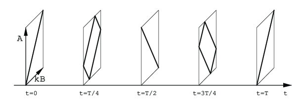
Figure 1: Oscillations of the piece-wise chiral string (53). When oscillating, string goes in successive sequence positions with the $T/4$ step, where the oscillation period $T=L/2$.

The first simple solvable example of a near stationary loop radiation is the multiply wound chiral string Davis2 :

$$\mathbf{a} \!=\! \frac{1}{m}\>(\cos m\xi,\;-\sin m\xi,\;0),$$

$$\mathbf{b} \!=\! \frac{k}{n}\>(\cos n\eta,\;-\cos\Phi\sin n\eta,\;-\sin\Phi\sin n\eta),$$ (44)

where $m,n$ are integer (harmonic numbers). For nonzero Fourier component indexes in (17) and (25) the following condition is held: $l=\kappa m=\lambda n$, where $\kappa$ and $\lambda$ are integers (see Appendix A for details). In all other cases $d\dot{E}^{\rm gr}_{l}/d\Omega=d\dot{E}^{\rm em}_{l}/d\Omega=0$. Let $\lambda$ be the minimum integer such as $\kappa m=\lambda n$. In this case first non-zero term in expanding of the energy on $k$ is proportional to $k^{2\lambda}$:

$$\dot{E}^{\rm gr} \simeq K^{\rm gr}(\kappa,\lambda,\Phi)l^{2}k^{2\lambda}G\mu^{2},$$

$$\dot{E}^{\rm em} \simeq K^{\rm em}(\kappa,\lambda,\Phi)l^{2}k^{2\lambda}q^{2}\mu,$$ (45)

where $K^{\rm gr}(\kappa,\lambda,\Phi)$ and $K^{\rm em}(\kappa,\lambda,\Phi)$ are numerical factors depending on geometrical string configuration. For example, the particular case with $m=n=1$ and $\Phi=0$ in (IV.1) corresponds to pure radial oscillations of the chiral loop:

$$\mathbf{a} = (\cos\xi,\;-\sin\xi,\;0),$$

$$\mathbf{b} = k(\cos\eta,\;-\sin\eta,\;0).$$ (46)

In this case the first non-zero term in expanding of radiated power on $k$ is proportional to $k^{2}$. Therefore taking into account only first term in expanding (17) we have (A)

$$I_{2}(1) \!\!=\!\! \frac{1}{2}\,e^{-i\phi}[J_{2}(-\sin\theta)+\!J_{0}(-\sin\theta)]\cos\theta,$$

$$I_{3}(1) \!\!=\!\! \frac{i}{2}\,e^{-i\phi}[J_{2}(-\sin\theta)-\!J_{0}(-\sin\theta)].$$ (47)

By keeping the leading nonzero term at $k\ll 1$ we obtain (A)

$$Y_{2}(1) = \frac{k}{2}\,e^{i\phi}\cos\theta,$$

$$Y_{3}(1) = i\frac{k}{2}\,e^{i\phi},$$

$$M(1) = \frac{k}{2}\,e^{i\phi}\sin\theta.$$ (48)

Substituting (IV.1) and (IV.1) in (III.1) and (32) we find

$$\frac{d\dot{E}^{\rm gr}}{d\Omega}\simeq\frac{G\mu^{2}\pi k^{2}}{2}\left\{\left[J_{2}(-\sin\theta)-J_{0}(-\sin\theta)\right]^{2}+\right.$$

$$2\left[3J^{2}_{2}(-\sin\theta)-J^{2}_{0}(-\sin\theta)\right]\cos^{2}\theta+$$

$$\left.\left[J_{2}(-\sin\theta)+J_{0}(-\sin\theta)\right]^{2}\cos^{4}\theta\right\},$$

$$\frac{d\dot{E}^{\rm em}}{d\Omega}\simeq\frac{\pi k^{2}q^{2}\mu}{8}\left\{\left[J_{2}(-\sin\theta)-J_{0}(-\sin\theta)\right]^{2}+\right.$$

$$\left.\left[J_{2}(-\sin\theta)+J_{0}(-\sin\theta)\right]^{2}\cos^{2}\theta\right\}\sin^{2}\theta.$$ (49)

Integration over the unit sphere in (IV.1) gives

$$K^{\rm gr}=\pi^{2}\int_{0}^{\pi}d\theta\sin\theta\left\{\left[J_{2}(\sin\theta)-J_{0}(\sin\theta)\right]^{2}+\right.$$

$$\left.2\left[3J^{2}_{2}(\sin\theta)-J^{2}_{0}(\sin\theta)\right]\cos^{2}\theta+\right.$$

$$\left.\left[J_{2}(\sin\theta)+J_{0}(\sin\theta)\right]^{2}\cos^{4}\theta\right\},$$

$$K^{\rm em}=\int_{0}^{\pi}d\theta\sin^{3}\theta\left\{\left[J_{2}(\sin\theta)-J_{0}(\sin\theta)\right]^{2}+\right.$$

$$\left.\left[J_{2}(\sin\theta)+J_{0}(\sin\theta)\right]^{2}\cos^{2}\theta\right\}.$$ (50)

with numerical values for $K^{\rm gr}=4.73$ and $K^{\rm em}=2.28$.

IV.2 Piece-wise string evolution

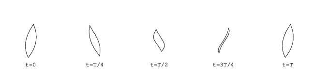
Figure 2: Projections of the stretched string loop (64) with an invariant length $L$ and oscillation period $T=L/2$ on the fixed two-dimensional plane. The string is shown in successive moments of time with the step of $T/4$. The small parameter $k$ is chosen to be equal $0.5$ for better visuality.

Let us consider now the second example of chiral string loop

$$\mathbf{a} = \mathbf{A}\left\{\begin{array}[]{lcl}\left(\xi-\pi/2\right),&&0\leq\xi\leq\pi,\\ \left(-\xi+3\pi/2\right),&&\pi\leq\xi\leq 2\pi,\\ \end{array}\right.$$ (53)

$$\mathbf{b} = k\mathbf{B}\left\{\begin{array}[]{lcl}\left(\eta-\pi/2\right),&&0\leq\eta\leq\pi,\\ \left(-\eta+3\pi/2\right),&&\pi\leq\eta\leq 2\pi,\\ \end{array}\right.$$ (56)

where $\mathbf{A}$ and $\mathbf{B}$ are constant unit vectors. This is the generalization of ordinary piece-wise string loop without the current Garfinkle to the chiral current case. See Fig. 1 for visualisation of this chiral loop oscillations. For fundamental integrals (III.1) and function $M(l)$ from (31) we obtain in this case respectively

$$I_{2}(l)\! = \!-\frac{i\mathbf{v}\mathbf{A}\left[e^{il\pi k\mathbf{n}\mathbf{B}/2}-(-1)^{l}e^{-il\pi k\mathbf{n}\mathbf{B}/2}\right]}{\pi l\left[1-(\mathbf{n}\mathbf{A})^{2}\right]},$$ (57)

$$I_{3}(l)\! = \!-\frac{i\mathbf{w}\mathbf{A}\left[e^{il\pi k\mathbf{n}\mathbf{B}/2}-(-1)^{l}e^{-il\pi k\mathbf{n}\mathbf{B}/2}\right]}{\pi l\left[1-(\mathbf{n}\mathbf{A})^{2}\right]},$$

$$Y_{2}(l) = \frac{ik\mathbf{v}\mathbf{B}\left[e^{il\pi k\mathbf{n}\mathbf{B}/2}-(-1)^{l}e^{-il\pi k\mathbf{n}\mathbf{B}/2}\right]}{\pi l\left[1-(k\mathbf{n}\mathbf{B})^{2}\right]},$$

$$Y_{3}(l)\! = \!\frac{ik\mathbf{w}\mathbf{B}\left[e^{il\pi k\mathbf{n}\mathbf{B}/2}-(-1)^{l}e^{-il\pi k\mathbf{n}\mathbf{B}/2}\right]}{\pi l\left[1-(k\mathbf{n}\mathbf{B})^{2}\right]},$$

$$M(l)\! = \!\frac{ik\mathbf{n}\mathbf{B}(1\!-\!k^{2})^{1/2}\!\left[e^{il\pi k\mathbf{n}\mathbf{B}/2}-(-1)^{l}e^{-il\pi k\mathbf{n}\mathbf{B}/2}\right]}{\pi l\left[1-(k\mathbf{n}\mathbf{B})^{2}\right]}.$$

Functions $Y_{p}(l)$ decrease here as $1/l$ with growing of $l$. Combining with similar behavior of $I_{p}(l)\propto 1/l$, this provides the convergence of energy series in (17) and (25). As a result for the gravitational and electromagnetic radiation of the nearly stationary chiral loop (53) we obtain respectively

$$\frac{d\dot{E}^{\rm gr}_{l}}{d\Omega} = \frac{32G\mu^{2}}{\pi^{3}l^{2}}\frac{\left[1-(-1)^{l}\cos(l\pi\mathbf{n}\mathbf{A})\right]\left[1-(-1)^{l}\cos(l\pi k\mathbf{n}\mathbf{B})\right]}{\left[1-(\mathbf{n}\mathbf{A})^{2}\right]\left[1-k^{2}(\mathbf{n}\mathbf{B})^{2}\right]^{2}}\left[1-(\mathbf{n}\mathbf{B})^{2}\right]k^{2},$$

$$\frac{d\dot{E}^{\rm em}_{l}}{d\Omega} = \frac{8q^{2}\mu}{\pi^{3}l^{2}}\frac{\left[1-(-1)^{l}\cos(l\pi\mathbf{n}\mathbf{A})\right]\left[1-(-1)^{l}\cos(l\pi k\mathbf{n}\mathbf{B})\right]}{\left[1-(\mathbf{n}\mathbf{A})^{2}\right]\left[1-k^{2}(\mathbf{n}\mathbf{B})^{2}\right]^{2}}(\mathbf{n}\mathbf{B})^{2}k^{2}(1-k^{2}),$$ (58)

$$\frac{d\dot{E}^{\rm gr}}{d\Omega} = \frac{16G\mu^{2}}{\pi}\frac{1-\frac{1}{2}\left(|\mathbf{n}\mathbf{A}+k\mathbf{n}\mathbf{B}|+|\mathbf{n}\mathbf{A}-k\mathbf{n}\mathbf{B}|\right)}{\left[1-(\mathbf{n}\mathbf{A})^{2}\right]\left[1-k^{2}(\mathbf{n}\mathbf{B})^{2}\right]^{2}}\left[1-(\mathbf{n}\mathbf{B})^{2}\right]k^{2},$$

$$\frac{d\dot{E}^{\rm em}}{d\Omega} = \frac{4q^{2}\mu}{\pi}\frac{1-\frac{1}{2}\left(|\mathbf{n}\mathbf{A}+k\mathbf{n}\mathbf{B}|+|\mathbf{n}\mathbf{A}-k\mathbf{n}\mathbf{B}|\right)}{\left[1-(\mathbf{n}\mathbf{A})^{2}\right]\left[1-k^{2}(\mathbf{n}\mathbf{B})^{2}\right]^{2}}(\mathbf{n}\mathbf{B})^{2}k^{2}(1-k^{2}).$$ (59)

The last two equations for the radiated energy flux into the solid angle $d\Omega$ are obtained after summation over $l$ with the using of identity Gradshteyn

$$\sum_{l=1}^{\infty}\frac{\cos(lx)}{l^{2}}=\frac{1}{4}(x-\pi)^{2}-\frac{\pi^{2}}{12},\quad 0\leq x\leq 2\pi.$$ (60)

Note, that (IV.2) and (IV.2) are valid for all $k$, not only for $k\ll 1$. Choosing $A=(1,0,0)$ and $B=(\cos\alpha,\,\sin\alpha,\,0)$ we find in this case from (43) the corresponding numerical factors $K^{\rm gr}$ and $K^{\rm em}$:

$$K^{\rm gr} \!\!=\!\! \frac{16}{\pi}\int_{0}^{\pi}\!\!\int_{0}^{2\pi}\!\!d\theta d\phi\sin\theta\frac{1\!-[\sin\theta\cos(\alpha-\phi)]^{2}}{1+|\cos\phi\sin\theta|},$$

$$K^{\rm em} \!\!=\!\! \frac{4}{\pi}\int_{0}^{\pi}\!\!\int_{0}^{2\pi}\!\!d\theta d\phi\sin\theta\frac{[\sin\theta\cos(\alpha-\phi)]^{2}}{1+|\cos\phi\sin\theta|}.$$ (61)

For example, in the particular case of $\alpha=\pi/2$ the double integrals (IV.2) equal $K^{\rm gr}=28.3$ and $K^{\rm em}=4$ respectively.

IV.3 Stretched loop oscillation

Let us consider now the loop of the following kind (combination of the first and second cases)

$$\mathbf{a} = \mathbf{A}\left\{\begin{array}[]{lcl}\left(\xi-\pi/2\right),&&0\leq\xi\leq\pi,\\ \left(-\xi+3\pi/2\right),&&\pi\leq\xi\leq 2\pi,\\ \end{array}\right.$$ (64)

$$\mathbf{b} = k(\sin\eta,\;-\cos\eta,\;0),$$ (65)

where $\mathbf{A}$ is the unit vector and $k\ll 1$. We will call this example as the stretched loop See Fig. 2. Substituting (IV.1) and (57) in (III.1), and integrating over the unit sphere, we find

$$K^{\rm gr}\!\!\! = \!\!\!\frac{12}{\pi}\!\int_{0}^{\pi}\!\!\int_{0}^{2\pi}\!\!\!d\theta\>d\phi\sin\theta\cos^{2}\theta\frac{[1+\cos\left(\pi\mathbf{n}\mathbf{A}\right)]^{2}}{1-(\mathbf{n}\mathbf{A})^{2}},$$

$$K^{\rm em}\!\!\! = \!\!\!\frac{1}{2\pi}\!\int_{0}^{\pi}\!\!\int_{0}^{2\pi}\!\!\!d\theta\>d\phi\sin^{3}\!\theta\frac{[1+\cos\left(\pi\mathbf{n}\mathbf{A}\right)]^{2}}{1-(\mathbf{n}\mathbf{A})^{2}}.$$ (66)

For example in the case $\mathbf{A}=(0,0,1)$ we find $K^{\rm gr}=7.63$ and $K^{\rm em}=3$.

V Damping of loop oscillations

Let us evaluate now the damping time of small amplitude oscillations of near stationary chiral strings corresponding to the limit $k\ll 1$ in (7). For simplicity we assume that $k$ does not depend on $\eta$ in the considered limit (this assumption is held true in the considered above solvable examples). Then a total loop charge conservation in (13) gives

$$\frac{q\sqrt{\mu}}{2}L\sqrt{1-k^{2}}=const.$$

From this equation we find the relation between energy $E$ and parameter $k$ of the chiral string with small amplitude oscillations:

$$E\simeq E_{v}\left(1+\frac{k^{2}}{2}\right),$$ (67)

where $E_{v}=L\mu$ is the energy of the stationary (vorton) chiral loop configuration at $k=0$. Comparing (67) with (42) we estimate the damping time of string oscillations

$$\tau\sim\frac{E_{v}}{2(K^{\rm gr}G\mu^{2}+K^{\rm em}q^{2}\mu)}.$$ (68)

Let us express (68) through vorton length. We have $E_{v}=L\mu$, where $L$ is the invariant length, and physical length of a stationary string is equal to half of invariant length $L_{\rm ph}=L/2$ Steer . We find

$$\tau\sim\frac{L_{\rm ph}}{K^{\rm gr}G\mu+K^{\rm em}q^{2}}.$$ (69)

In the case of the chiral ring with one harmonic (IV.1), it is naturally to assume, that evolving ring saves its form (due to symmetry) during the damping of small amplitude oscillations. In this case therefore we can find precisely the evolution of the radiating string with time. Only $k$ varies in time if the shape of the string is invariable. Solving together (42) and (67), we find the law of oscillation damping in the near stationary chiral ring

$$k^{2}\simeq k^{2}_{0}e^{-t(1/\tau_{c}^{\rm gr}+1/\tau_{c}^{\rm em})},$$ (70)

where $k_{0}=k(t=0)$, and correspondingly the damping time due to gravitational radiation

$$\tau_{c}^{\rm gr} = \frac{E_{v}}{2K^{\rm gr}G\mu^{2}}=\frac{L_{\rm ph}}{K^{\rm gr}G\mu}$$ (71)

and due to electromagnetic radiation

$$\tau_{c}^{\rm em} = \frac{E_{v}}{2K^{\rm em}q^{2}\mu}=\frac{L_{\rm ph}}{K^{\rm em}q^{2}}.$$ (72)

Substituting (70) in (67) we obtain

$$E\simeq E_{v}\left[1+\frac{k^{2}_{0}}{2}e^{-t(1/\tau_{c}^{\rm gr}+1/\tau_{c}^{\rm em})}\right].$$ (73)

An effective number of oscillations during the damping time (oscillator quality) is

$$Q=\frac{\tau}{T}=\frac{2}{L}\frac{\tau^{\rm gr}\tau^{\rm em}}{\tau^{\rm gr}+\tau^{\rm em}}.$$ (74)

To restore the usual CGS units we replace $G\mu^{2}\rightarrow G\mu^{2}c$, $q^{2}\mu\rightarrow q^{2}\mu c^{2}/\hbar$ and choose standard normalization for the string mass per unit length $G\mu/c^{2}=10^{-6}\mu_{6}$ and $q_{e}=q/e$ for dimensionless charge carrier on the string, where elementary electric charge is $e=4.8\times 10^{-10}$. As a result we obtain for damping time

$$\tau^{\rm gr}=\frac{L_{\rm ph}c}{K^{\rm gr}G\mu},\quad\tau^{\rm em}=\frac{L_{\rm ph}\hbar}{K^{\rm em}q^{2}}.$$ (75)

The oscillator quality (74) in the cases of the gravitational and electromagnetic radiation are respectively

$$Q^{\rm gr}=\frac{1}{K^{\rm gr}}\frac{c^{2}}{G\mu},\quad Q^{\rm em}=\frac{1}{K^{\rm em}}\frac{1}{\alpha_{\rm em}q_{e}^{2}},$$ (76)

with $\alpha_{\rm em}=e^{2}/c\hbar$ The ratio of damping times is

$$\tau^{\rm gr}/\tau^{\rm em}\sim\frac{q^{2}}{G\mu\hbar}\left(\frac{K^{\rm em}}{K^{\rm gr}}\right)\simeq 1.4\times 10^{-4}\frac{q_{e}^{2}}{\mu_{6}}\frac{K^{\rm em}}{K^{\rm gr}}.$$ (77)

If $q_{e}^{2}/\mu_{6}\gtrsim 1.4\times 10^{-3}$, then electromagnetic radiation prevails in the chiral loop evolution (it is valid for the standard values of $\mu_{6}\sim 1$ and $q_{e}\sim 1$). If on the contrary $q_{e}^{2}/\mu_{6}\lesssim 1.4\times 10^{-3}$ (for example, if a current is neutral and there is no electromagnetic radiation at all), then pure gravitational radiation determines the evolution.

Let us estimate a characteristic size of the string $L_{\rm v}$ with oscillation damping time (75) equals to the universe lifetime $t_{0}\simeq 10^{18}$ s. In the case of the gravitational radiation predominance we find

$$L_{\rm v}^{\rm gr}\simeq\frac{G\mu K^{\rm gr}t_{0}}{c}\simeq 10^{2}\mu_{6}\mbox{ kpc}$$ (78)

for $K^{\rm gr}\sim 1$. So the chiral strings with length $L<L_{\rm v}^{\rm gr}$ (i. e. with a size of typical galactic halo or less) have had enough time to fade into vortons. On the other hand if the electromagnetic radiation prevails, we have

$$L_{\rm v}^{\rm em}\simeq\frac{q^{2}K^{\rm em}t_{0}}{\hbar}\simeq 70q_{e}^{2}\mbox{ Mpc}$$ (79)

for $K^{\rm em}\sim 1$ and so the electromagnetically radiated chiral loops with the length shorter than the size of galactic clusters have had transformed now to vortons.

VI Discussion

We have explored the asymptotic fading of chiral cosmic string loops into vortons. It turns out that the upper bound of the gravitational radiation of a near stationary loop (40) is proportional to the squared third derivative of the oscillation amplitude. This result is in qualitative agreement with the known formula for gravitational radiation in quadruple approximation.

The derived equations (III.1) and (32) for respectively the gravitational and electromagnetic power radiation of oscillating chiral loops are suitable for practical calculations. We demonstrate that, if oscillations are small in amplitude ($k\ll 1$) and the current $j^{\mu}$ is constant along the string, then the power of the gravitational and electromagnetic radiation (42) is proportional to $k^{2}$ and the coefficient of proportionality depends only on the form of the loop. For some examples of chiral loops we calculated the total radiated power in the limit of small amplitude oscillations. For chiral ring with small amplitude radial oscillations the radiated power per solid angle $d\Omega$ for the electromagnetic (IV.2) and gravitational (IV.2) radiation is found analytically.

We estimated the damping time of chiral loops (68) with small amplitude oscillations. In the case of the gravitational radiation prevalence this time is $\tau^{\rm gr}\sim L_{\rm ph}/K^{\rm gr}G\mu$, where $K^{\rm gr}$ is a numerical coefficient depending on the string geometry. The damping time due to the gravitational radiation of the considered chiral loops is of the order of magnitude longer than the lifetime of ordinary cosmic strings. If the electromagnetic radiation is prevail then decay time is $\tau^{\rm em}\sim L_{\rm ph}/K^{\rm em}q^{2}$. The oscillation energy and amplitude parameter $k$ of the radially oscillating chiral ring are found to be exponentially decaying with time according to respectively (70) and (73).

From the damping time estimation it follows that only sufficiently long superconducting cosmic strings oscillate up to the present time. On the contrary the small scale chiral loops transformed into the stationary vortons due to the oscillation damping. Namely, the minimal length of presently oscillating chiral loop varies from $L_{\rm v}^{\rm gr}\sim 10^{2}\mu_{6}$ kpc for gravitational radiation domination to $L_{\rm v}^{\rm em}\sim 70q_{e}^{2}$ Mpc for electromagnetic radiation domination depending on the relations between $\mu$ and $q$. It appears that the oscillator quality of chiral loops (76) is independent on the loop length and is determined only by the loop shape through geometric parameters $K^{\rm gr}$ and $K^{\rm em}$. For characteristic values of $K^{\rm gr}\sim 10$ and $K^{\rm em}\sim 1$ the corresponding oscillator qualities for the gravitational and electromagnetic radiation are $Q^{\rm gr}\sim 10^{5}/\mu_{6}$ and $Q^{\rm em}\sim 137/q_{e}^{2}$.

Appendix A Multiply wound ring

Here we calculate the fundamental integrals (22), (23) and (31) which define the radiated power of the string for the particular case of multiply wound loop in the Section IV.1. We begin from the consideration of the following integrals

$$Is_{lm}(x,y)\!\! =\!\! \frac{1}{2\pi}\!\int_{0}^{2\pi}\!\!\!\!d\eta e^{il(\eta+x\sin m\eta+y\cos m\eta)}\sin\eta,$$

$$Ic_{lm}(x,y)\!\! = \!\!\frac{1}{2\pi}\!\int_{0}^{2\pi}\!\!\!\!d\eta e^{il(\eta+x\sin m\eta+y\cos m\eta)}\cos\eta.\quad$$ (80)

The combinations $Is_{lm}\pm Ic_{lm}$ are integrals of the form

$$S_{nm}(x,y)=\frac{1}{2\pi}\int_{0}^{2\pi}\!\!d\eta e^{il(\eta+x\sin m\eta+y\cos m\eta)},$$ (81)

and integral (81) is expressed as follows

$$S_{nm}(x,y)\!=\!\left\{\begin{array}[]{ll}\!\left(\frac{x-iy}{r}\right)^{n/m}T_{nm}(nr),&r\neq 0,\\ \!0,&r=0,n\neq 0,\\ \!1,&r=0,n=0,\end{array}\right.$$ (82)

where $r=(x^{2}+y^{2})^{1/2}$ and

$$T_{nm}(r)=\frac{1}{2\pi}\int_{0}^{2\pi}d\eta e^{i(n\eta+r\sin m\eta)}.$$ (83)

Let $n,m$ are integer. If $n=cm$, where $c$ is integer, then replacing $\eta\rightarrow m\eta$ and taking into account, that the function in integral (83) is periodic we find

$$T_{nm}(r)=J_{c}(-r),\quad n=cm,\quad n,m,c\in Z,$$ (84)

where $J_{c}$ is $c$-th Bessel function. Then integrals (A) can be expressed through Bessel functions in the following way

$$Is_{nm}\!\! =\!\! -\frac{i}{2}\!\left(\frac{z^{*}}{r}\right)^{c}\left[\frac{z^{*}}{r}J_{c+1}(-cr)-\!\frac{z}{r}J_{c-1}(-cr)\right]\!,$$

$$Ic_{nm}\!\! =\!\! \frac{1}{2}\!\left(\frac{z^{*}}{r}\right)^{c}\left[\frac{z^{*}}{r}J_{c+1}(-cr)+\!\frac{z}{r}J_{c-1}(-cr)\right]\!,\quad$$ (85)

where $z=x+iy$ and $z^{*}=x-iy$. Let us demonstrate now that if $n\neq cm$, where $c$ is integer, then integrals (A) equal zero. In other words we need to prove, that $T_{nm}(r)\equiv 0$ if $n\neq cm$. First of all we note that

$$f(\eta)={\rm Im}\,e^{i(n\eta+r\sin m\eta)}=-f(2\pi-\eta)$$ (86)

and therefore ${\rm Im}\,T_{nm}(r)\equiv 0$. The real part of function in the integral (83) is

$$\cos n\eta\cos(r\sin m\eta)-\sin n\eta\sin(r\sin m\eta).$$ (87)

Expansion of $\cos(r\sin m\eta)$ and $\sin(r\sin m\eta)$ in Taylor series gives:

$$\cos(r\sin m\eta) = \sum_{k=0}^{\infty}(-1)^{k}\frac{(r\sin m\eta)^{2k}}{2k!},$$

$$\sin(r\sin m\eta) = \sum_{k=0}^{\infty}(-1)^{k}\frac{(r\sin m\eta)^{2k+1}}{(2k+1)!},$$ (88)

where for odd and even values of $k$ we have the standard binomial-like representation

$$\sin^{k}m\eta=\!\left(\frac{1}{2i}\right)^{k-1}\left[\sin km\eta\!-\!C_{1}^{k}\sin(k\!-\!2)m\eta\!+...+\!(-1)^{\frac{k-1}{2}}C_{(k-1)/2}^{k}\sin m\eta\right],$$

$$\sin^{k}m\eta=\!\frac{(-1)^{\frac{k}{2}}}{2^{k-1}}\left[\cos km\eta\!+...+\!(-1)^{\frac{k-1}{2}}C_{(k-1)/2}^{k}\cos 2m\eta\right]\!+\!\frac{1}{2^{k}}C_{k/2}^{k}.\,$$ (89)

It can be seen that only terms of the kind

$$\int_{0}^{2\pi}\!\!\!d\eta\,\sin(n\eta)\,\sin[(2k+1)m\eta],$$

$$\int_{0}^{2\pi}\!\!\!d\eta\,\cos(n\eta)\,\cos(2km\eta),$$ (90)

enter in the considered series (A). Using this fact and (86) we find, that if $n\neq cm$, where $c$ is integer, then integrals (A) equal zero, what we wanted to prove.

Let us consider the following chiral circular loop:

$$\mathbf{a} \!=\! \frac{1}{m}(\cos m\xi-\sin m\xi),$$

$$\mathbf{b} \!\!\!=\!\!\! \frac{k}{n}(\cos n\eta-\cos\Phi\sin n\eta-\sin\Phi\sin n\eta),\quad$$ (91)

where $m,n$ are integer. For $l=\kappa m$, where $\kappa$ is integer, we obtain (see (A,A))

$$I_{2}(l) \!\!=\!\! \frac{1}{2}\cos\theta[J_{\kappa+1}(-\kappa\sin\theta)\!+\!J_{\kappa-1}(-\kappa\sin\theta)]e^{-i\kappa\phi},$$

$$I_{3}(l) \!\!=\!\! \frac{i}{2}[J_{\kappa+1}(-\kappa\sin\theta)\!-\!J_{\kappa-1}(-\kappa\sin\theta)]e^{-i\kappa\phi}.$$ (92)

For all others $l$ we have $I_{p}(l)=0$. Denoting further $x=k\>\sin\theta\>\cos\phi$, $y=k(\cos\Phi\>\sin\theta\>\sin\phi+\sin\Phi\>\cos\theta)$, $r=(x^{2}+y^{2})^{1/2}$, we can write

$$Y_{2}(l) \!\!=\!\! k\cos\theta\cos\phi Ic_{l,n}(-x,y)$$

$$+k(\cos\Phi\cos\theta\sin\phi-\sin\Phi\sin\theta)Is_{l,n}(-x,y),$$

$$Y_{3}(l) \!\!=\!\! -k\sin\phi Ic_{l,n}(-x,y)+k\cos\Phi\cos\phi Is_{l,n}(-x,y),$$

$$M(l) \!\!=\!\! S_{l,n}(-x,y)\sqrt{1-k^{2}}.$$ (93)

If $l=\lambda n$, where $\lambda$ is integer, then $Y_{p}\neq 0$, $M(l)\neq 0$, In all other cases $Y_{p}=M(l)=0$. As a result: if $l=\kappa m=\lambda n$ (where $\kappa$, $\lambda$ are integer), then $l$-th term in expanding of the energy is nonzero. In all other cases $d\dot{E}^{\rm gr}_{l}/d\Omega=d\dot{E}^{\rm em}_{l}/d\Omega=0$. Let $\lambda$ is minimal integer, such as $\kappa m=\lambda n$. From the properties of Bessel functions

$$J_{l}(x)=\frac{x^{l}}{2^{l}l!}+O(x^{2}),$$ (94)

it follows for (82) and (A) in the first nonzero term of expansion on $k$:

$$Is_{ln} = \frac{i}{2}(-x-iy)^{\lambda-1}\frac{(-\lambda)^{\lambda-1}}{2^{\lambda-1}(\lambda-1)!},$$

$$Ic_{ln} = \frac{1}{2}(-x-iy)^{\lambda-1}\frac{(-\lambda)^{\lambda-1}}{2^{\lambda-1}(\lambda-1)!},$$

$$S_{ln} = (-x-iy)^{\lambda}\frac{(-\lambda)^{\lambda}}{2^{\lambda}(\lambda)!}.$$ (95)

Using (A), we obtain (A)

$$Y_{2}(l) \!=\! \frac{k}{2}(-x-iy)^{\lambda-1}\frac{(-\lambda)^{\lambda-1}}{2^{\lambda-1}(\lambda-1)!}\times$$

$$\left(\cos\theta\cos\phi+i\cos\Phi\cos\theta\sin\phi-i\sin\Phi\sin\theta\right),$$

$$Y_{3}(l) \!=\! \frac{k}{2}(-x-iy)^{\lambda-1}\frac{(-\lambda)^{\lambda-1}}{2^{\lambda-1}(\lambda-1)!}\times$$

$$\left(-\sin\phi+i\cos\Phi\cos\phi\right),$$

$$M(l) = (-x-iy)^{\lambda}\frac{(-\lambda)^{\lambda}}{2^{\lambda}(\lambda)!}\sqrt{1-k^{2}}.$$ (96)

By substituting (A) in (III.1) and (32) we can calculate the corresponding parameter $\Gamma$ from expressions for $\dot{E}^{\rm gr}=\Gamma^{\rm gr}G\mu^{2}$ and $\dot{E}^{\rm em}=\Gamma^{\rm em}G\mu^{2}$.

References

• (1) T. W. B. Kibble, J. Phys. A 9, 1387 (1976); T. W. B. Kibble, G. Lazarides and Q. Shafi, Phys. Rev. D 26, 435 (1982)
• (2) Y. B. Zel’dovich, Mon. Not. R. Astron. Soc. 192, 663 (1980)
• (3) A. Vilenkin, Phys. Rev. D 24, 2082 (1981); A. Vilenkin, Phys. Rep. 121, 263 (1985)
• (4) E. Witten, Nucl. Phys. B249, 557 (1985)
• (5) R. L. Davis and E. P. S. Shellard, Phys. Lett. B209, 485 (1988)
• (6) D. Haws, M. Hindmarsh and N. Turok, Phys. Lett. B209, 255 (1988)
• (7) E. Copeland, D. Haws, M. Hindmarsh and N. Turok, Nucl. Phys. B306, 908 (1988)
• (8) E. P. S. Shellard and A. Vilenkin, Cosmic Strings and other Topological Defects (Cambridge University Press, Cambridge, England, 1994)
• (9) M. B. Hindmarsh and T. W. B. Kibble, Rep. Prog. Phys. 58, 477 (1995)
• (10) B. Carter and P. Peter, Phys. Lett. B466, 41 (1999)
• (11) A. C. Davis, T. W. B. Kibble, M. Pickles and D.A. Steer, Phys. Rev. D 62 (2000) 083516
• (12) J.J. Blanco-Pillado, Ken D. Olum and A. Vilenkin, Phys. Rev. D 63, 103513
• (13) J.J. Blanco-Pillado and Ken D. Olum, Nucl. Phys. B599 (2001) 435
• (14) V. Berezinsky, B. Hnatyk and A. Vilenkin, Phys. Rev. D 64 (2001) 043004
• (15) J.M. Quashnock and D.N. Spergel, Phys. Rev. D 42 (1990) 2505
• (16) S. Weinberg, Gravitation and Cosmology (Wiley, New York, 1974)
• (17) R. Durrer, Nucl. Phys. B328, 238 (1989)
• (18) D. Garfinkle and T Vachaspati, Phys. Rev. D 36, 2229 (1987)
• (19) I.S. Gradshteyn and I.M. Ryzhik, Tables of Integrals, Series and Products (Academic, New York, 1980)
• (20) D.A. Steer, Phys.Rev. D 63, (2001) 083517
• (21) L.D. Landau and E.M. Lifshitz, The Classical Theory of Fields.
• (22) A. Vilenkin and T. Vachaspati, Phys.Rev.Lett 58, 1041 (1987)