Thermodynamic limit of the canonical partition function with respect to the quark number in QCD

Abstract

We investigate QCD in the canonical ensemble with respect to the quark number. We reveal that the canonical description in which the quark number is fixed would be reduced to the grand canonical description under the thermodynamic limit. Since the grand canonical ensemble contains fluctuations of the quark number, the idea of the canonical ensemble is of no use for the purpose of defining order parameters for the deconfinement transition. We clarify the origin of such reduction and propose an idea to define the order parameter. The Monte-Carlo simulation by means of the spin system, which is an effective model of QCD at finite temperature, shows prosperous behavior though the results suffer from the severe statistical error due to the sign problem.

I INTRODUCTION

Extensive efforts have been shedding light upon the phase structure of Quantum Chromodynamics (QCD) at finite temperature, though there remain many subtleties yet. The center symmetry is a prosperous implement to characterize the deconfinement transition in pure non-abelian gauge theories (gauge theories without dynamical quarks) sve82 . The order parameter to examine whether the symmetry is broken or not is the expectation value of the Polyakov loop pol78 , that is, the Wilson line winding around the Euclidean thermal torus. The Polyakov loop vanishes in the confined phase, while it takes a finite value in the deconfined phase. In pure gauge theories the critical properties associated with the deconfinement transition have been ascertained by the lattice Monte-Carlo simulations. The results are in accord with those anticipated from the center symmetry and the universality argument mcl81 .

In contrast to pure gauge theories any definite indicator in order to distinguish the deconfined phase from confined one is not established so far yet for systems including dynamical quarks in the fundamental representation. Once the thermal excitation of light quarks is allowed, the center symmetry is broken explicitly. If we construct a 3-d effective model in terms of the order parameter, namely the Polyakov loop, in the presence of dynamical quarks, those quark contributions bring about an external magnetic-like field acting onto the Polyakov loop, which breaks the center symmetry ban83 . Then it is obvious that the Polyakov loop is no longer a proper indicator for confinement because it remains finite even in the confined phase as well as in the deconfined phase due to the absence of the center symmetry.

We note, however, that the notion of confinement should be still articulate even when dynamical quarks are present simply because it is an experimental fact. To find out an appropriate indicator to identify the confined phase in the presence of dynamical quarks it is essential to clarify where the dynamical screening against the Polyakov loop should originate from. In fact, DeTar and McLerran det82 argued that some fractional excitations of dynamical quarks are responsible for the explicit breaking of the center symmetry and proposed a new order parameter for the deconfinement transition based on the canonical description with respect to the quark triality or quark number. This idea had been deserted since Meyer-Ortmanns mey84 showed that DeTar–McLerran’s order parameter behaves unexpectedly and always indicates the confining character for the Z(2) Higgs model on the lattice. Although Meyer-Ortmanns has explicitly demonstrated a failure in the proposed order parameter in the model study, it is not apparent in principle what would cause DeTar–McLerran’s formulation not to fulfill the naive expectation as a proper order parameter. Similar ideas for the deconfinement order parameter based on the canonical ensemble have been proposed and discussed by several authors also wei87 ; ole92 ; fab95 but those arguments are essentially integrated into DeTar–McLerran’s first insight.

Interestingly enough, we can find a clear-sighted comment in Meyer-Ortmanns’ paper as follows: “The states at zero temperature have a finite particle number hence zero particle density, while the relevant states at finite temperature have finite particle density. Therefore one cannot check whether there exist states at zero temperature with fractional baryon number by looking at what states contribute to the partition function at finite temperature.” In her analysis on the Z(2) Higgs model, we can discern no clear embodiment for the statement quoted above. Nevertheless, we would emphasize that this point is actually the most critical in constructing the order parameter for the deconfinement transition. The purpose of the present paper is to give a simple and transparent demonstration to disclose what becomes of the partition function with the particle number kept fixed under the thermodynamic limit.

The problem here can be also stated in more general grounds. The question is whether the grand canonical description with zero quark chemical potential is equivalent to the canonical description with zero quark number or not. We will find that the canonical description with zero quark number would amount to the canonical description with zero quark density whenever the thermodynamic limit is taken. As a result, DeTar–McLerran’s idea to project out the fractional excitations of dynamical quarks does not work because the states with zero particle density may have any fractional excitation of particles which becomes irrelevant eventually in the thermodynamic limit. Then by all means can we reach the desired canonical ensemble in which the particle number is fixed at zero? We will propose one possibility in the present work.

This paper is organized as follows: In Sec. II we review DeTar–McLerran’s idea from the point of view of the canonical ensemble with respect to the quark number. Sec. III is devoted to investigating the thermodynamic limit of the canonical partition function. Using the simplest example we elucidate analytically and numerically that the canonical partition function would be reduced to the conventional grand canonical one under the thermodynamic limit. We reveal the cause of the failure in defining an order parameter for the deconfinement transition. In Sec. IV, we propose an idea to overcome the problem in connection with taking the thermodynamic limit. Performing the Monte-Carlo simulation, we put the idea to the test to confirm that our order parameter would be prosperous. We also find that the problem of constructing an order parameter for the deconfinement transition is deeply related to the sign problem of the Dirac determinant. The results of the numerical simulations suffer from the severe statistical errors due to the sign problem. The concluding remarks are in Sec. V.

II IDEA OF THE CANONICAL ENSEMBLE

II.1 Canonical ensemble with respect to the quark number

We will briefly review the idea of the canonical ensemble with emphasis on the possibility to define an order parameter for the deconfinement transition.

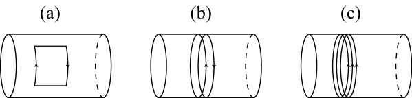
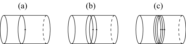
Figure 1: Typical examples of the thermal excitations of dynamical quarks which respect the center symmetry. The torus represents the thermal $S^{1}$ and the spatial $R^{3}$. (a) Creation and annihilation process of a quark ($q$) and an antiquark ($\bar{q}$). (b) Mesonic excitation composed of $q\bar{q}$. (c) Baryonic excitation composed of $qqq$ in the case of $N_{\mathrm{c}}=3$.

Figure 2: Typical examples of the thermal excitations of dynamical quarks which break the center symmetry. (a) Single quark ($q$) excitation. (b) $qq$ excitation. (c) Mesonic and single quark ($q\bar{q}q$) excitation.

First of all, we should notice that the conventional QCD partition function at finite temperature and zero density is implicitly formulated in the grand canonical ensemble with zero quark chemical potential, that is equivalent to the canonical ensemble with zero quark density under the thermodynamic limit. This fact is easily understood as follows. In the imaginary-time formalism of the finite-temperature field theories, the temporal (thermal) extent is compactified to the inverse temperature. Then, in addition to the pair excitations of a quark and an antiquark as depicted in Fig. 2 (a), isolated quark excitations as shown in Fig. 2 (a) also satisfy the quark current conservation and thus the quark number can fluctuate thermally. In the thermodynamic limit, however, the quark number conservation is recovered because only the states with zero quark number dominate the partition function at vanishing chemical potential. This point of view has already been discussed in Ref. azc98 and it seems reasonable from the principle of the statistical mechanics.

Usually it does not matter in calculating physical observables whether such fractional excitations of dynamical quarks are present. The situation may be totally different for the manifestation of the center symmetry. In the language of the lattice gauge theory, the center symmetry is defined as the invariance under the center transformation, that is, the transformation from the temporal link variables $U_{4}(x_{4}=N_{\tau})$ on a time slice altogether into $z\cdot U_{4}(x_{4}=N_{\tau})$, where $z$ is an element of the center of the gauge group (Z(3) for the SU(3) gauge theory). For the quark thermal contributions the Z(3) factor $z$ is multiplied every time dynamical quarks wind around the thermal torus. Thus thermal excitations gathered typically in Fig. 2 are center symmetric because $z\cdot z^{\dagger}=z^{3}=1$ for $z\in Z(3)$. Thermal excitations shown in Fig. 2 are, on the other hand, typical examples which break the center symmetry. Then, what happens if we exclude any thermal excitation like those in Fig. 2 by using the canonical description where the quark number is fixed? Once we employ the canonical ensemble with zero quark number, for example, only such excitations as shown in Fig. 2 (a) (b) are allowed so that the canonical partition function would regain the center symmetry. Certainly the symmetry itself is explicitly broken in the Lagrangian and nevertheless the physical states remain center symmetric. Owing to the recovered symmetry, we can presume that the Polyakov loop will provide a criterion for the deconfinement transition in the same way as in the case of pure gauge theories. Essentially, this is the idea proposed originally by DeTar and McLerran in Ref. det82 .

The canonical description of QCD at finite density is available by the Legendre transformation from the quark chemical potential $\mu$ to the quark number $n_{q}$ eng99 . (In this paper we simply write the quark number to mean the quark number minus the antiquark number.) For later convenience, we explain the transformation procedures in some mathematical details. To make our calculation tangible, we adopt the Wilson fermion on the lattice from now on. The final results, of course, can be understood not only in a specific formalism but in a general way also.

The quark number density is the fourth component of the conserved current given by

$$j_{4}(x)=\kappa\{\bar{\psi}(x)(1-\gamma_{4})U_{4}(x)\psi(x+\hat{4})-\bar{\psi}(x+\hat{4})(1+\gamma_{4})U_{4}^{\dagger}(x)\psi(x)\},$$ (1)

where $\kappa$ is the hopping parameter and the Wilson parameter is chosen as $r=1$ for the sake of simplicity. By imposing the constraint onto the configurations we can write the canonical partition function with respect to the quark number $n_{q}$ as

$$Z_{\text{CE}}(n_{q}) =\int\mathcal{D}U\mathcal{D}\bar{\psi}\mathcal{D}\psi\,\mathrm{e}^{-S_{\text{G}}[U]-S_{\text{F}}[U,\bar{\psi},\psi]}\,\delta\biggl{(}\frac{1}{N_{\tau}}\sum_{x}j_{4}(x)-n_{q}\biggr{)}$$

$$=\int_{0}^{2\pi}\frac{\mathrm{d}\phi}{2\pi}\,\mathrm{e}^{-\mathrm{i}n_{q}\phi}\int\mathcal{D}U\mathcal{D}\bar{\psi}\mathcal{D}\psi\,\mathrm{e}^{-S_{\text{G}}[U]-S_{\text{F}}[U,\bar{\psi},\psi]+\mathrm{i}\frac{\phi a}{\beta}\sum j_{4}(x)},$$ (2)

where $S_{\text{G}}[U]$ is the gluon action and $S_{\text{F}}[U,\bar{\psi},\psi]$ is the action of the Wilson fermion with $r=1$. The lattice spacing $a$ and the number of lattices along the temporal direction $N_{\tau}$ give the inverse temperature, i.e., $\beta=N_{\tau}a$. The quark parts of the action are put together as

$$-S_{\text{F}}[U,\bar{\psi},\psi]+\mathrm{i}\frac{\phi a}{\beta}\sum_{x}j_{4}(x)$$

$$= -\sum_{x}\biggl{\{}\bar{\psi}(x)\psi(x)-\kappa\sum_{j}\bigl{[}\bar{\psi}(x)(1-\gamma_{j})U_{j}(x)\psi(x+\hat{j})+\bar{\psi}(x+\hat{j})(1+\gamma_{j})U_{j}^{\dagger}(x)\psi(x)\bigl{]}$$

$$-\kappa\biggl{[}\Bigl{(}1\!+\!\mathrm{i}\frac{\phi a}{\beta}\Bigr{)}\bar{\psi}(x)(1\!-\!\gamma_{4})U_{4}(x)\psi(x\!+\!\hat{4})+\Bigl{(}1\!-\!\mathrm{i}\frac{\phi a}{\beta}\Bigr{)}\bar{\psi}(x\!+\!\hat{4})(1\!+\!\gamma_{4})U_{4}^{\dagger}(x)\psi(x)\biggr{]}\biggr{\}}.$$ (3)

Here $\mathrm{i}\phi$ can be regarded as an imaginary chemical potential and the integration over $\phi$ corresponds to the Legendre transformation from the chemical potential to the quark number eng99 . $\hat{j}$ runs from $\hat{1}$ to $\hat{3}$ in the spatial directions. In the same way as the usual prescription to treat the chemical potential in the lattice gauge theories has83 we exponentiate the imaginary chemical potential as follows;

$$1+\mathrm{i}\frac{\phi a}{\beta}\sim\exp\Bigl{(}\mathrm{i}\frac{\phi a}{\beta}\Bigr{)},\qquad 1-\mathrm{i}\frac{\phi a}{\beta}\sim\exp\Bigl{(}-\mathrm{i}\frac{\phi a}{\beta}\Bigr{)},$$ (4)

which makes only higher order corrections of $\mathrm{O}(a^{2})$. The fundamental reason to demand the above prescription is because of the gauge invariance, or the center symmetry in the present case. With these alterations the partition function given by Eq. (2) becomes exactly center symmetric for $n_{q}=0,\pm 3,\pm 6,\dots(0\mod 3)$ as it should be. In order to see it apparently, transforming the quark fields by

$$\psi^{\prime}(x)=\mathrm{e}^{\mathrm{i}\frac{\phi a}{\beta}x_{4}}\psi(x),\qquad\bar{\psi}^{\prime}(x)=\mathrm{e}^{-\mathrm{i}\frac{\phi a}{\beta}x_{4}}\bar{\psi}(x),$$ (5)

we rewrite the quark action in terms of the transformed fields as eng99

$$\!-\tilde{S}_{\text{F}}[U,\bar{\psi}^{\prime},\psi^{\prime}]$$

$$\!+\kappa\!\sum_{\vec{x}}\Bigl{[}\mathrm{e}^{\mathrm{i}\phi}\bar{\psi}^{\prime}(\vec{x},N_{\tau})(1\!-\!\gamma_{4})U_{4}(\vec{x},N_{\tau})\psi^{\prime}(\vec{x},1)\!+\!\mathrm{e}^{-\mathrm{i}\phi}\bar{\psi}^{\prime}(\vec{x},1)(1\!+\!\gamma_{4})U_{4}^{\dagger}(\vec{x},N_{\tau})\psi^{\prime}(\vec{x},N_{\tau})\Bigr{]}.$$ (6)

$\tilde{S}_{\text{F}}[U,\bar{\psi},\psi]$ is the rest of the action from which the terms involving $U_{4}(\vec{x},N_{\tau})$ are subtracted. It is obvious that the center transformation $U_{4}(\vec{x},N_{\tau})\to\mathrm{e}^{\mathrm{i}2\pi k/3}U_{4}(\vec{x},N_{\tau})$ is equivalent to the shift of $\phi$ by $2\pi k/3$. We can immediately recognize from Eq. (2) that the canonical partition function is certainly invariant under $\phi\to\phi+2\pi k/3$ as long as the quark number satisfies $n_{q}=0\mod 3$.

The integration of the partition function in terms of $\phi$ exactly corresponds to the decomposition of the Dirac determinant into each part with fixed quark winding number. This is seen transparently if the Dirac determinant obtained from the quark action Eq. (6), that is denoted by $\det D[U,\phi]$ from now on, is calculated by means of the hopping parameter expansion. The expanded terms are represented by closed quark paths similarly as depicted in Figs. 2 and 2. Every time the quark path winds around the thermal torus, it picks up the factor $\mathrm{e}^{\mathrm{i}\phi}$ so that the Dirac determinant can be decomposed according to the quark number $n_{q}$;

$$\det D[U,\phi]=\sum_{n_{q}=-\infty}^{\infty}\mathrm{e}^{\mathrm{i}n_{q}\phi}\det D^{(n_{q})}[U],$$ (7)

where $\det D^{(n_{q})}[U]$ is the part of the Dirac determinant with the quark path winding $n_{q}$ times around the thermal torus. Thus the integration over $\phi$ in Eq. (2) singles out some specific combinations of the operators coming from the Dirac determinant under the condition that the quark winding number is fixed. This result is not particular to the case of the Wilson fermion formalism on the lattice. In general, the canonical partition function is given by

$$Z_{\text{CE}}(n_{q})=\int_{0}^{2\pi}\frac{\mathrm{d}\phi}{2\pi}\,\mathrm{e}^{-\mathrm{i}n_{q}\phi}\int\mathcal{D}U\det D[U,\phi]\,\mathrm{e}^{-S_{\text{G}}[U]}$$ (8)

with the Dirac determinant $\det D[U,\phi]$ under the twisted boundary conditions,

$$\psi(\vec{x},x_{4}=\beta)=-\mathrm{e}^{\mathrm{i}\phi}\psi(\vec{x},x_{4}=0),\qquad\bar{\psi}(\vec{x},x_{4}=\beta)=-\mathrm{e}^{-\mathrm{i}\phi}\bar{\psi}(\vec{x},x_{4}=0).$$ (9)

It leads to the canonical partition function in the same sense as in Ref. ole92 , that is, the partition function with the Dirac determinant replaced by its specific part with some fixed quark excitations. It is interesting that the constraint onto the configurations, imposed by Dirac’s delta function, results in the restriction onto the combination of the operators after all. This is because of the non-local character of the quark (fermion) fields.

II.2 DeTar–McLerran’s order parameter

Here we will explicitly construct DeTar–McLerran’s order parameter for the deconfinement transition. They introduced the quark triality $t_{q}$ defined as $n_{q}\mod 3$ and considered the canonical partition function with respect to $t_{q}$. It is available from the canonical partition function with respect to $n_{q}$ as

$$\tilde{Z}_{\text{CE}}(t_{q}) =\sum_{m=-\infty}^{\infty}Z_{\text{CE}}(n_{q}=3m+t_{q})$$

$$=\frac{1}{3}\sum_{\phi=0,\pm 2\pi/3}\mathrm{e}^{-\mathrm{i}t_{q}\phi}\int\mathcal{D}U\det D[U,\phi]\,\mathrm{e}^{-S_{\text{G}}[U]}.$$ (10)

Then DeTar–McLerran’s order parameter is given by

$$\mathcal{\tilde{P}_{N}}=\frac{\tilde{Z}_{\text{CE}}(t_{q}=\mathcal{N})}{\sum_{t_{q}}\tilde{Z}_{\text{CE}}(t_{q})}$$ (11)

for arbitrary $\mathcal{N}\neq 0$. When the quark number is fixed instead of the quark triality, we can define also in the same way as

$$\mathcal{P_{N}}=\frac{Z_{\text{CE}}(n_{q}=\mathcal{N})}{\sum_{n_{q}}Z_{\text{CE}}(n_{q})},$$ (12)

which is expected to behave similarly to $\mathcal{\tilde{P}_{N}}$. In the confined phase where all the physical excitations are color-neutral, any thermal excitation of isolated quarks would cost infinitely large energy. Therefore it follows that $\tilde{Z}_{\text{CE}}(t_{q}=\mathcal{N})=Z_{\text{CE}}(n_{q}=\mathcal{N})=0$ for $\mathcal{N}\neq 0\mod 3$. After the dynamical breaking of the center symmetry occurs, fractional quark excitations are allowed at finite energies so that the canonical partition function can take a non-vanishing value. Hence, $\mathcal{\tilde{P}_{N}}$ and $\mathcal{P_{N}}$ are anticipated to serve as order parameters for the deconfinement transition.

We can manipulate the order parameter in other forms comparable with the conventional definition, namely the Polyakov loop. As discussed in Refs. ole92 ; fab95 , the expectation value of the Polyakov loop itself can be expected to be a proper order parameter in the canonical ensemble. Because the center symmetry becomes manifest in the canonical partition function with the quark number $n_{q}=0\mod 3$ (or the quark triality $t_{q}=0$), the deconfinement transition could be characterized by the dynamical breaking of the center symmetry. Thus another candidate for an order parameter for the deconfinement transition is given by $\langle\widetilde{\mathrm{tr}L(\vec{x})}\rangle_{\text{CE}}$ with $t_{q}=0$, that is,

$$\langle\widetilde{\mathrm{tr}L(\vec{x})}\rangle_{\text{CE}}=\frac{\frac{1}{3}\sum_{\phi}\int\mathcal{D}U\det D[U,\phi]\,\mathrm{e}^{-S_{\text{G}}[U]}\,\mathrm{tr}L(\vec{x})}{\tilde{Z}_{\text{CE}}(t_{q}=0)}.$$ (13)

In the same way as in the case of $\mathcal{\tilde{P}_{N}}$ a similar variation is also possible for $\langle\widetilde{\mathrm{tr}L(\vec{x})}\rangle_{\text{CE}}$, i.e., we can consider $\langle\mathrm{tr}L(\vec{x})\rangle_{\text{CE}}$ with $n_{q}=0$ for example as

$$\langle\mathrm{tr}L(\vec{x})\rangle_{\text{CE}}=\frac{\int_{0}^{2\pi}\frac{\mathrm{d}\phi}{2\pi}\int\mathcal{D}U\det D[U,\phi]\,\mathrm{e}^{-S_{\text{G}}[U]}\,\mathrm{tr}L(\vec{x})}{Z_{\text{CE}}(n_{q}=0)},$$ (14)

where $L(\vec{x})$ stands for the Polyakov loop defined by

$$L(\vec{x})=\mathcal{T}\exp\biggl{[}-\mathrm{i}g\int_{0}^{\beta}\mathrm{d}x_{4}\,A_{4}(x_{4})\biggr{]}.$$ (15)

Here $\mathcal{T}$ represents the time-ordering and $A_{4}(x)$ is the temporal component of gauge fields.

We can explicitly evaluate the integration with respect to $\phi$ once the actual form of $\det D[U,\phi]$ is given. Now we will exploit the hopping parameter expansion. Following the calculation of Ref. gre84 the Dirac determinant amended by $\phi$ can be readily expanded in the lowest order of the hopping parameter expansion as follows;

$$\det D[U,\phi]=\exp\biggl{[}H\sum_{\vec{x}}\bigl{\{}\mathrm{e}^{\mathrm{i}\phi}\mathrm{tr}L(\vec{x})+\mathrm{e}^{-\mathrm{i}\phi}\mathrm{tr}L^{\dagger}(\vec{x})\bigr{\}}\biggr{]},$$ (16)

where $H=2(2\kappa)^{N_{\tau}}$ and $L(\vec{x})$ here is the Polyakov loop defined on the lattice by

$$L(\vec{x})=\prod_{x_{4}=a}^{N_{\tau}a}U_{4}(\vec{x},x_{4}),$$ (17)

which can be graphically represented like in Fig. 2 (a). With the notations $M=\sum\mathrm{tr}L(\vec{x})=|M|\,\mathrm{e}^{\mathrm{i}\theta_{M}}$, the integration in terms of $\phi$ in Eq. (2) results in mil87

$$\int_{0}^{2\pi}\frac{\mathrm{d}\phi}{2\pi}\,\mathrm{e}^{-\mathrm{i}n_{q}\phi}\cdot\mathrm{e}^{H(\mathrm{e}^{\mathrm{i}\phi}M+\mathrm{e}^{-\mathrm{i}\phi}M^{\dagger})}=\mathrm{e}^{\mathrm{i}n_{q}\theta_{M}}I_{n_{q}}(2H|M|),$$ (18)

where $I_{\nu}(x)$ is the modified Bessel function of the first kind. By differentiating the integrand with respect to $\phi$, we can have the expression for the expectation value of the quark number as

$$n_{q}=\langle HM\rangle_{n_{q}-1}-\langle HM^{\dagger}\rangle_{n_{q}+1}.$$ (19)

This relation can be confirmed analytically also by the formula $I_{\nu-1}(x)-I_{\nu+1}(x)=(2\nu/x)I_{\nu}(x)$. Also it can be expressed as $n_{q}=2\mathrm{i}H\mathrm{Im}\langle\sum\mathrm{tr}L(\vec{x})\mathrm{e}^{\mathrm{i}\phi}\rangle_{n_{q}}$. This form of the relation has been found already in Ref. mil87 . It would be worth mentioning that a different but similar relation has been discussed also in a numerical way in Ref. for00 , which suggests that the above relation could persist beyound the leading order of the hopping parameter expansion.

In the lowest order of the hopping parameter expansion, we can write down DeTar–McLerran’s order parameter as

$$\mathcal{P_{N}}=\frac{\int\mathcal{D}U\,\mathrm{e}^{-S_{\text{G}}[U]+\mathrm{i}\mathcal{N}\theta_{M}}I_{\mathcal{N}}(2H|M|)}{\int\mathcal{D}U\,\mathrm{e}^{-S_{\text{G}}[U]+2H|M|\cos\theta_{M}}}.$$ (20)

As for the expectation value of the Polyakov loop in the canonical ensemble, we can immediately write down as

$$\langle\mathrm{tr}L\rangle_{\text{CE}}=\frac{1}{V}\frac{\int\mathcal{D}U\,\mathrm{e}^{-S_{\text{G}}[U]+\mathrm{i}\theta_{M}}I_{0}(2H|M|)\,|M|}{\int\mathcal{D}U\,\mathrm{e}^{-S_{\text{G}}[U]}I_{0}(2H|M|)}.$$ (21)

In the next section, we address the problem of taking the thermodynamic limit for these would-be order parameters (20) and (21). The point will turn out that the sum of the Polyakov loop $M=\sum\mathrm{tr}L(\vec{x})$ is an extensive quantity and as large as proportional to the volume.

III THERMODYNAMIC LIMIT

III.1 Failure as order parameters

We consider the thermodynamic limit here, that is, we make the system volume go to infinity. Then we will find that both $\mathcal{P_{N}}$ and $\langle\mathrm{tr}L\rangle_{\text{CE}}$ fail serving as order parameters for the deconfinement transition. Roughly speaking, the failure as order parameters stems from fractional quark excitations permitted even in the canonical ensemble under the infinite volume limit. As schematically depicted in Fig. 3, a pair of a quark and an antiquark can be excited (drawn by the thin curves) because such an excitation is mesonic and the net quark number is zero. When the distance between source quarks (drawn by the thick curves) gets large, it would be regarded as the system composed of two mesonic excitations as shown in the left figure of Fig. 3. In the limit of the infinite distance between source quarks, two mesonic excitations should become individual (clustering decomposing property as shown in the right figure of Fig. 3), which means that the Polyakov loop associated with a single quark excitation can be effectively screened by the fractional excitation of dynamical quarks. Although any fractional excitation of dynamical quarks is prohibited at first by the definition of the canonical ensemble, it would be allowed eventually in the infinitely large volume limit due to the clustering decomposing property. As a result, $\mathcal{P}_{\mathcal{N}\neq 0}$ amounts to non-zero $\mathcal{P}_{\mathcal{N}=0}$ and $\langle\mathrm{tr}L\rangle_{\text{CE}}$ is reduced to the Polyakov loop expectation value in the conventional grand canonical ensemble under the thermodynamic limit.

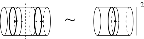
Figure 3: The schematic picture for the emergence of fractional quark excitations allowed even in the canonical ensemble under the thermodynamic limit.

Let us confirm the above intuitive understanding in the actual expressions given by Eqs. (20) and (21). Without any spontaneous breaking of the center symmetry, $\mathcal{P_{N}}$ is expected to vanish for $\mathcal{N}\neq 0\mod 3$. This expected property derives from the integration with respect to $\theta_{M}$ in Eqs. (20) and (21). Owing to the projection by the integration over $\phi$, the partition function depends on $\theta_{M}$ only through the factor $\mathrm{e}^{\mathrm{i}\mathcal{N}\theta_{M}}$. Therefore, if $\mathcal{N}$ takes a non-zero value, the integration with respect to $\theta_{M}$ makes zero as a result of the whole average over the phase factor. Unless external perturbation is introduced, $\mathcal{P}_{\mathcal{N}\neq 0}=0$ should be maintained even in the thermodynamic limit. In other words, any spontaneous breaking of the symmetry cannot be described without external perturbation. Thus even after taking the thermodynamic limit, we have vanishing $\mathcal{P}_{\mathcal{N}\neq 0}$ in the absence of external perturbation regardless of whether the system lies in the confined or deconfined phase. This is what Meyer-Ortmanns found in her analysis.

In the presence of small perturbation denoted by $h$, the phase factor is modified to $\mathrm{e}^{\mathrm{i}\mathcal{N}\theta_{M}+2h|M|\cos\theta_{M}}$. In the thermodynamic limit, $|M|$ may become as large as proportional to the volume and then only the stationary point $\theta_{M}=0$ dominates the integration with respect to the Polyakov loop. Consequently $\mathcal{P_{N}}$ loses any $\mathcal{N}$ dependence to lead to $\mathcal{P_{N}}\neq 0$ for arbitrary $\mathcal{N}$. In other words, the regained center symmetry is always broken and the partition function is reduced into that in the grand canonical ensemble in which the center symmetry is explicitly broken whenever small perturbation is introduced in order to realize the spontaneous symmetry breaking. Thus the situation is sharply contrast to Meyer-Ortmanns’ analysis. Once external perturbation is applied, the canonical description resolves itself into the grand canonical description. If we deal carefully with the thermodynamic limit and try to retain the canonical description, even the spontaneous breaking of the center symmetry becomes unavailable. In any case, the state of affairs is somewhat of antinomy.

In order to gain a deeper insight, we will deal with a toy model in which the Polyakov loop dynamics is emulated by the spin system in the next subsection.

III.2 A toy model

In this subsection we investigate the thermodynamic limit of the canonical ensemble by means of the Ising model as a toy tool. The argument of the center symmetry tells us that the Polyakov loop dynamics can be effectively described by the Ising model with the Z(2) symmetry for the SU(2) gauge theory and by the Potts model with the Z(3) symmetry for the SU(3) gauge theory. In fact, such an effective description has been established also in the numerical study sve97 .

For simplicity, we will focus here on the Ising model with the Z(2) symmetry, though the discussion is easily extended to the case of the Potts model. The counterpart for the order parameter (20) can be immediately expressed in terms of the spin variables as

$$\mathcal{P}_{-1}^{\text{Ising}}=\frac{\sum_{\langle s\rangle}\mathrm{e}^{-J\sum s_{n}s_{m}}\frac{1}{2}\bigl{(}\mathrm{e}^{H\sum s_{n}}-\mathrm{e}^{-H\sum s_{n}}\bigr{)}}{\sum_{\langle s\rangle}\mathrm{e}^{-J\sum s_{n}s_{m}+H\sum s_{n}}}$$ (22)

with the exchange interaction $J$ between the nearest neighbor sites under a magnetic field $H$. Also the counterpart for the order parameter (21) can be written as

$$\langle s\rangle_{\text{CE}}^{\text{Ising}}=\frac{1}{V}\frac{\sum_{\langle s\rangle}\mathrm{e}^{-J\sum s_{n}s_{m}}\frac{1}{2}\bigl{(}\mathrm{e}^{H\sum s_{n}}+\mathrm{e}^{-H\sum s_{n}}\bigr{)}\,\sum s_{n}}{\sum_{\langle s\rangle}\mathrm{e}^{-J\sum s_{n}s_{m}}\frac{1}{2}\bigl{(}\mathrm{e}^{H\sum s_{n}}+\mathrm{e}^{-H\sum s_{n}}\bigr{)}}.$$ (23)

For the purpose of investigating what happens in the thermodynamic limit, it will be sufficient to consider the simplest case in which the exchange interaction is absent ($J=0$). Then the order parameters given by Eqs. (22) and (23) can be exactly evaluated, namely, they are trivially zero. The naive expectation is that these order parameters remain zero while the magnitude of the exchange interaction is small, regardless of the presence of an external magnetic field $H\neq 0$. They will come to take a finite value when the strength of the interaction grows large enough to bring about the dynamical symmetry breaking. Actually, however, this naive expectation is not realized at all. We must follow the standard procedure to describe the spontaneous symmetry breaking; we add an infinitesimal external field denoted by $h$ and then take the thermodynamic limit ($V\to\infty$) and finally turn off the external field ($h\to 0$). The order parameters under an infinitesimal external field $h$ is calculated for $J=0$ as

$$\mathcal{P}_{-1}^{\text{Ising}} =\frac{\sum_{\langle s\rangle}\frac{1}{2}\bigl{(}\mathrm{e}^{(H+h)\sum s_{n}}-\mathrm{e}^{-(H-h)\sum s_{n}}\bigr{)}}{\sum_{\langle s\rangle}\mathrm{e}^{(H+h)\sum s_{n}}}$$

$$=\frac{\bigl{(}2\cosh(H+h)\bigr{)}^{V}-(2\cosh(H-h)\bigr{)}^{V}}{2\bigl{(}2\cosh(H+h)\bigr{)}^{V}}$$

$$\to\frac{1}{2}\qquad(V\to\infty,\quad H\gg h>0).$$ (24)

We can draw the similar result for another candidate, that is,

$$\langle s\rangle_{\text{CE}}^{\text{Ising}} =\frac{1}{V}\frac{\sum_{\langle s\rangle}\frac{1}{2}\bigl{(}\mathrm{e}^{(H+h)\sum s_{n}}+\mathrm{e}^{-(H-h)\sum s_{n}}\bigr{)}\sum s_{n}}{\sum_{\langle s\rangle}\frac{1}{2}\bigl{(}\mathrm{e}^{(H+h)\sum s_{n}}+\mathrm{e}^{-(H-h)\sum s_{n}}\bigr{)}}$$

$$=\frac{\bigl{(}2\cosh(H+h)\bigr{)}^{V-1}2\sinh(H+h)-\bigl{(}2\cosh(H-h)\bigr{)}^{V-1}2\sinh(H-h)}{\bigl{(}2\cosh(H+h)\bigr{)}^{V}+\bigl{(}2\cosh(H-h)\bigr{)}^{V}}$$

$$\to\tanh(H+h)\qquad(V\to\infty,\quad H\gg h>0).$$ (25)

The above results of Eqs. (24) and (25) clearly signify that the would-be order parameters given by Eqs. (22) and (23) are to be disqualified under the thermodynamic limit because they always remain finite. In other words, any expectation value calculated in the canonical ensemble in which the center symmetry is seemingly recovered would be reduced into that calculated in the grand canonical ensemble in which the symmetry is explicitly broken. The point is that the contribution among the projective superposition with respect to $\phi$ survives only when it is parallel to the direction of the external magnetic field. As a result, the projection into the canonical ensemble is diminished only to result in the same description as in the grand canonical ensemble. We can intuitively understand the situation in the following way: In the thermodynamic limit, the projective superposition in Eq. (23) for example becomes

$$\mathrm{e}^{H\sum s_{n}}+\mathrm{e}^{-H\sum s_{n}}\to\mathrm{e}^{H|\sum s_{n}|},$$ (26)

which follows that the spin configurations for which $\mathrm{e}^{H\sum s_{n}}$ dominates should be definitely separated from the spin configuration for which $\mathrm{e}^{-H\sum s_{n}}$ does, that is, the system becomes non-ergodic. Which term survives in the thermodynamic limit depends on which direction an external field is introduced in.

The same mechanism makes the canonical ensemble in QCD be unstable under the thermodynamic limit. For the configuration of the Polyakov loop with a macroscopic order, $M=\sum\mathrm{tr}L(\vec{x})=|M|\,\mathrm{e}^{\mathrm{i}\theta_{M}}\sim\mathrm{O}(V)\to\infty$, the integration with respect to $\phi$ in Eq. (18) becomes

$$\int_{0}^{2\pi}\frac{\mathrm{d}\phi}{2\pi}\,\mathrm{e}^{-\mathrm{i}n_{q}\phi}\cdot\mathrm{e}^{H(\mathrm{e}^{\mathrm{i}\phi}M+\mathrm{e}^{-\mathrm{i}\phi}M^{\dagger})}=\int_{0}^{2\pi}\frac{\mathrm{d}\phi}{2\pi}\,\mathrm{e}^{-\mathrm{i}n_{q}\phi}\cdot\mathrm{e}^{2H|M|\cos(\phi+\theta_{M})}$$

$$\simeq \frac{\sqrt{2\pi}\,\mathrm{e}^{-\mathrm{i}n_{q}\phi_{0}}\cdot\mathrm{e}^{2H|M|\cos(\phi_{0}+\theta_{M})}}{2\pi\bigl{|}-2H|M|\cos(\phi_{0}+\theta_{M})\bigr{|}^{\frac{1}{2}}}\Biggl{|}_{\phi_{0}=-\theta_{M}}\qquad(|M|\sim\mathrm{O}(V)\to\infty).$$ (27)

In the last line of the above equations only the leading order of the saddle-point approximation ($2H\cos(\phi_{0}+\theta_{M})$ is maximized at $\phi_{0}=-\theta_{M}$) is left, which becomes exact when $|M|$ goes to infinity. The meaning of the saddle-point approximation in Eq. (27) is absolutely the same as what Eq. (26) means. Then infinitesimal perturbation like the $h$ field in Eqs. (24) and (25) forces only specific $\theta_{M}$ to be favored in the thermodynamic limit. Thus neither DeTar–McLerran’s order parameter nor the Polyakov loop expectation value in the canonical ensemble would serve as a proper order parameter for the deconfinement transition.

IV IDEA TO OVERCOME THE PROBLEM

IV.1 Prospect as order parameters

So far we have clarified why DeTar–McLerran’s order parameter does not work as expected under the thermodynamic limit. Nevertheless, we have prospects of making use of DeTar–McLerran’s order parameter to identify the deconfinement transition. The idea is quite simple. The spin-system counterpart for DeTar–McLerran’s order parameter given in Eq. (22) can be equivalently expressed in the following form:

$$\mathcal{P}_{-1}^{\text{Ising}}=\frac{\frac{1}{2}\langle\mathrm{e}^{H\sum s_{n}}-\mathrm{e}^{-H\sum s_{n}}\rangle_{J}}{\langle\mathrm{e}^{H\sum s_{n}}\rangle_{J}},$$ (28)

where $\langle\cdots\rangle_{J}$ denotes the ensemble average with the action $-J\sum s_{n}s_{m}$. Let us imagine that we compute the order parameter of Eq. (28) by the method of the Monte-Carlo simulation. First we generate the ensemble of configurations with the probability specified by the action $-J\sum s_{n}s_{m}$, which has both the symmetric phase with random alignments and the broken phase with a spontaneous magnetization. Next we calculate the ensemble average with those generated configurations. In the symmetric phase, the numerator of Eq. (28) should vanish, while it take a finite value in the broken phase. Hence it is apparent that the would-be order parameter given in Eq. (28) will serve as a proper order parameter. If we prefer the spin expectation value to DeTar–McLerran’s formulation, it would be enough to rewrite Eq. (23) into

$$\langle s\rangle_{\text{CE}}^{\text{Ising}}=\frac{1}{V}\frac{\langle\bigl{(}\mathrm{e}^{H\sum s_{n}}+\mathrm{e}^{-H\sum s_{n}}\bigr{)}\sum s_{n}\rangle_{J}}{\langle\mathrm{e}^{H\sum s_{n}}+\mathrm{e}^{-H\sum s_{n}}\rangle_{J}}.$$ (29)

What is important here is that the probability for configurations is specified by the symmetric part of the action. If we adopt the whole action, for example $-J\sum s_{n}s_{m}+\ln\cosh(H\sum s_{n})$ for Eq. (23), to generate the configurations, the ensemble of configurations becomes non-ergodic in the thermodynamic limit and the would-be order parameters should inevitably fail as demonstrated in Eqs. (24) and (25). In other words, the ensemble of configurations given by $-J\sum s_{n}s_{m}+\ln\cosh(H\sum s_{n})$ is unstable against configurations with $\sum s_{n}\sim\mathrm{O}(V)$ because of the long-ranged nature of the interaction term $\ln\cosh(H\sum s_{n})$. As a result the spin configurations with $\sum s_{n}>0$ is completely decoupled from those with $\sum s_{n}<0$ and the canonical description is reduced to the grand canonical one.

The above idea is quite simple in itself. In the rest of this subsection, we will discuss the physical meaning of the above prescription to generate the ensemble of configurations with the probability specified by the symmetric part of the action.

Looking back at the argument around Eq. (27), let us reconsider the validity for the saddle-point approximation which is expected to be exact in the thermodynamic limit. Once $|M|$ is really as large as of order $\mathrm{O}(V)$, the argument given in Eq. (27) has no suspicious controversy at all. However, going back to the second line of Eq. (2), we realize that the coefficient in front of $\phi$ is at most $n_{q}$ which is now of order $\mathrm{O}(1)$. If we considered the thermodynamic limit where we take $n_{q}\sim\mathrm{O}(V)\to\infty$ with the number density $n_{q}/V$ fixed, the aforementioned argument of the saddle-point approximation would become exact and the calculation of the canonical ensemble is absolutely identical as that in the grand canonical one, as closely discussed in Ref. hag85 . Then the expectation value of the phase of the Polyakov loop is finite and almost proportional to the quark number density for00 , as seen in Eq. (19).

As we have already emphasized, the canonical ensemble for the purpose of characterizing the deconfinement transition is different. What we should be confronted with is the ensemble where $n_{q}$ is fixed at so small number of order $\mathrm{O}(1)$ that the saddle-point approximation would be inapplicable. So as to realize this situation an additional condition is needed; $|M|=|\sum\mathrm{tr}L(\vec{x})|$ must be kept of order $\mathrm{O}(1)$. This condition can be achieved in the form of the ensemble average in Eqs. (28) and (29) as numerically demonstrated in the next subsection.

We shall summarize our findings and assertions here again.

• Even when the quark number is fixed in the canonical formulation, it is the quark number density that is actually fixed under the thermodynamic limit because the system becomes unstable against configurations with a macroscopic order. Thus any fluctuation of the quark number of order $\mathrm{O}(1)$ is allowed even in the canonical description, though it is unintended. As a result the notion of confinement becomes obscured.

• The idea is simple: If we completely get rid of the fluctuation of the quark number, which is negligible in the thermodynamic limit but responsible for screening the Polyakov loop, the canonical ensemble with respect to the quark number is expected to recover its meaning. Then DeTar–McLerran’s order parameter and also the Polyakov loop should serve as order parameters for the deconfinement transition.

• The fluctuation of the quark number is induced by the infinitely non-local interaction arising from the projective superposition. Such fluctuation can be excluded by taking the ensemble average with configurations generated by the symmetric part of the action. The asymmetric part of the action is regarded as included in the operator part to be averaged over.

IV.2 Numerical tests

By using the Monte-Carlo simulation, we numerically calculate Eq. (29) which can be comparable with an ordinary magnetization in the presence of an external magnetic field. The lattice size is chosen as $100\times 100$ and we adopt the standard Metropolis algorithm. The strengths of the exchange interaction and the magnetic field are $J=0.5/T$ and $H=0.1/T$ respectively, where $T$ is the temperature. The thermalization of the spin system is well achieved after 10000 times sweeps, as can be confirmed by the magnetization distributions shown in Fig. 4 for $T=0.5$ and $T=2.0$. It should be noted that the magnetization is typically of order $\mathrm{O}(V)$ in the ordered phase ($T=0.5$) and of order $\mathrm{O}(1)$ in the disordered phase ($T=2.0$).

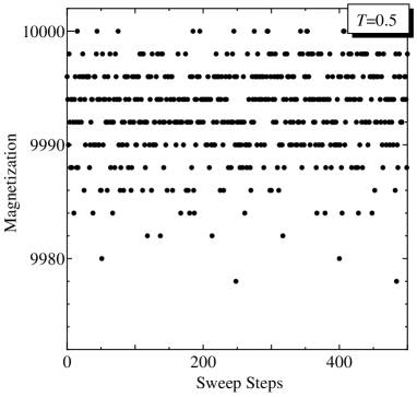
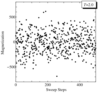
Figure 4: Magnetization at each sweep step after the thermalization achieved by 10000 times sweeps. The left figure is for $T=0.5$ in the ordered phase and the right for $T=2.0$ in the disordered phase.

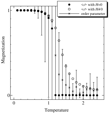
Figure 5: Behaviors of the magnetizations and the order parameter as functions of the temperature.

The resultant $\langle s\rangle_{\text{CE}}^{\text{Ising}}$ is presented in Fig. 5. Filled circles stand for the spontaneous magnetization in the case of $H=0$ and indicate that the spin system goes through the second-order phase transition at $T_{\text{c}}=2.27J=1.13$ (theoretical value). Blank circles represent the magnetization in the presence of the magnetic field $H\neq 0$ and show a smooth crossover as the temperature raises. We plot $\langle s\rangle_{\text{CE}}^{\text{Ising}}$ by crosses with error-bars. Although we take 10000 samples by each 10 intervals, the statistical error is still large because the term $\mathrm{e}^{H\sum s_{n}}+\mathrm{e}^{-H\sum s_{n}}$ in both the numerator and the denominator of Eq. (29) can become so large that the operator to be taken the ensemble average of must furiously fluctuate to lead to large statistical errors. In a sense we can say that this problem of slow convergence arises from the same origin as that of the sign problem for simulations at finite density, in particular, the situation is alike the Glasgow method in lattice QCD at finite density. This parallelism to the sign problem will be more apparent for the order parameter given by Eq. (28) or Eq. (20). As discussed in Sec. III the canonical partition function can vanish due to the average over the phase factor coming from the Dirac determinant.

The results shown in Fig. 5 seem to suggest that the would-be order parameter $\langle s\rangle_{\text{CE}}^{\text{Ising}}$ should work as expected. Unfortunately, at this stage, we cannot address any stronger statement due to large statistical errors. In order to improve the accuracy, some essential ingenuity such as a reweighting method fod01 are needed rather than simple accumulation of many samples. That is beyond the scope of the present paper.

IV.3 Construction of the order parameter in QCD

It is easy to write down the QCD counterparts for the order parameters given by Eqs. (28) and (29) in the spin system. Here we present the expressions only for DeTar–McLerran’s order parameter defined by Eq. (11) and the Polyakov loop expectation value given by Eq. (13). The formulation can be straightforwardly extended to general cases.

The quark contribution from the Dirac determinant can be expressed as the effective action in the following form;

$$\det D[U]=\mathrm{e}^{-S_{\text{eff}}[U,U_{4}(x_{4}=N_{\tau})]},$$ (30)

where the link variable $U_{4}(x_{4}=N_{\tau})$ receiving a modification under the center transformation is explicitly written for convenience. We can decompose the effective action according to the triality, that is,

$$S_{\text{eff}}^{(k)}[U]=\frac{1}{3}\sum_{n=0,\pm 1}\,\mathrm{e}^{-\mathrm{i}2\pi kn/3}\,S_{\text{eff}}[U,z_{0}^{n}U_{4}(x_{4}=N_{\tau})]\qquad(k=0,\pm 1)$$ (31)

with $z_{0}=\mathrm{e}^{\mathrm{i}2\pi/3}\in\mathrm{Z}(3)$. Among the decomposed parts, all the contributions with non-trivial triality ($k=\pm 1$) are bound to be included in the operator to be averaged over. Therefore the would-be order parameter given by Eq. (11) can be written for $\mathcal{N}=1$ as

$$\tilde{\mathcal{P}}_{1}=\frac{\frac{1}{3}\Bigl{\langle}\mathrm{e}^{-S_{\text{eff}}^{(1)}-S_{\text{eff}}^{(-1)}}+z_{0}^{-1}\mathrm{e}^{-z_{0}S_{\text{eff}}^{(1)}-z_{0}^{-1}S_{\text{eff}}^{(-1)}}+z_{0}\,\mathrm{e}^{-z_{0}^{-1}S_{\text{eff}}^{(1)}-z_{0}S_{\text{eff}}^{(-1)}}\Bigr{\rangle}_{\text{sym}}}{\Bigl{\langle}\mathrm{e}^{-S_{\text{eff}}^{(1)}-S_{\text{eff}}^{(-1)}}\Bigr{\rangle}_{\text{sym}}}.$$ (32)

The ensemble average is to be taken with the probability weight specified by the symmetric part of the action, i.e., $-S_{\text{G}}[U]-S_{\text{eff}}^{(0)}[U]$. In the same way, the expression for Eq. (13) can be written as

$$\langle\widetilde{\mathrm{tr}L(\vec{x})}\rangle_{\text{CE}}=\frac{\Bigl{\langle}\bigl{(}\mathrm{e}^{-S_{\text{eff}}^{(1)}-S_{\text{eff}}^{(-1)}}+\mathrm{e}^{-z_{0}S_{\text{eff}}^{(1)}-z_{0}^{-1}S_{\text{eff}}^{(-1)}}+\mathrm{e}^{-z_{0}^{-1}S_{\text{eff}}^{(1)}-z_{0}S_{\text{eff}}^{(-1)}}\bigr{)}\,\mathrm{tr}L(\vec{x})\Bigr{\rangle}_{\text{sym}}}{\Bigl{\langle}\mathrm{e}^{-S_{\text{eff}}^{(1)}-S_{\text{eff}}^{(-1)}}+\mathrm{e}^{-z_{0}S_{\text{eff}}^{(1)}-z_{0}^{-1}S_{\text{eff}}^{(-1)}}+\mathrm{e}^{-z_{0}^{-1}S_{\text{eff}}^{(1)}-z_{0}S_{\text{eff}}^{(-1)}}\Bigr{\rangle}_{\text{sym}}}.$$ (33)

V CONCLUDING REMARKS

In order to identify the deconfinement phase transition we employed and elaborated the idea of the canonical ensemble with respect to the quark number or triality. We clarify why the canonical ensemble would be reduced into the grand canonical ensemble eventually in the thermodynamic limit. In order to overcome the problem of the thermodynamic limit, we propose a prescription to compute the ensemble average. The idea is tested by means of an effective model in terms of spin variables in the presence of the magnetic field. The results seem prosperous but turn out to suffer from the severe sign problem. Although our definition of the order parameter for the deconfinement transition can be applied to the Monte-Carlo simulation on the lattice, it is inevitably necessary to get over the sign problem inherent in the lattice QCD at finite density. We find it interesting that two serious questions – one is the criterion for the deconfinement transition at finite temperature, and the other is the sign problem in the lattice QCD at finite density – are closely related to each others.