MPI-PhT/2002-14
hep-ph/0204299
April 2002

HEAVY QUARKONIUM DYNAMICS 

An introduction to the recent developments in perturbative heavy quarkonium physics is given. Covered are the effective theories NRQCD, pNRQCD and vNRQCD, the threshold expansion, the role of renormalons, and applications to bottom and top quark physics.

1 Introduction

The study of non-relativistic two-body systems consisting of a heavy quark-antiquark ($Q\bar{Q}$) pair has a long tradition since the discovery of the $J/\psi$ and the work of Appelquist and Politzer,$\!{}^{{\bf?}}$ which had shown that, owing to asymptotic freedom, non-relativistic quantum mechanics should apply to a good approximation to heavy $Q\bar{Q}$ systems. Thus, heavy quarkonium systems should be predominantly Coulomb-like bound states sharing many features of positronium and an ideal tool studying the interplay of perturbative and non-perturbative aspects of quantum chromodynamics (QCD).

The realization of this idea has proven a difficult task. Not even to the first approximation does the Balmer spectrum of QED give a good quantitative description of the charmonium or bottomonium spectrum. It was found that perturbation theory completely fails to describe the long distance part of the heavy quark potential. Subsequently, potential models emerged,$\!{}^{{\bf?}}$ which incorporated a linear rising potential at long distances in accordance to the idea of quark confinement $\!{}^{{\bf?}}$ and a Coulomb-like potential at short distances in accordance to perturbation theory. Potential models were highly successful in describing the observed spectra and transition rates, but they were not derived from first principles in QCD. As such they cannot be used for quantitative tests of QCD.

On the other hand, it was found that non-perturbative effects in heavy quarkonia, where the quark mass $m$ is sufficiently large, such that $m\gg mv\gg mv^{2}\gg\Lambda_{\rm QCD}$, $v$ being the quark velocity and $\Lambda_{\rm QCD}$ the typical hadronization scale, can be described by an operator product expansion in terms of local and gauge-invariant quark and gluon condensates.$\!{}^{{\bf?},{\bf?},{\bf?}}$ Only the top-antitop quark system truly belongs into this category. For bottomonia, the ground states and, maybe, low radial excitations might belong to this category too, but mesons containing charm do certainly not. However, even for the perturbative contributions for systems in this category, it was not straightforward to systematically determine higher orders corrections, either due to ultraviolet (UV) divergences in approaches starting from the non-relativistic approximation, or due to the amount of technical difficulties in the relativistic approach, the Bethe-Salpeter formalism.$\!{}^{{\bf?}}$

A new conceptual approach using an effective field theory was proposed by Caswell and Lepage $\!{}^{{\bf?}}$ and Bodwin, Braaten and Lepage. $\!{}^{{\bf?}}$ These authors found that, for the description of quarkonia, QCD can be reformulated in terms of an effective non-renormalizable Lagrangian built from quark and gluonic field operators describing fluctuations below $m$, whereas hard effects associated with the scale $m$ are incorporated in the coefficients of the operators. The theory is called “non-relativistic QCD” (NRQCD). At present, NRQCD is one of the standard instruments to describe quarkonium production and decay properties at collider experiments. In NRQCD, production and decay of quarkonia is described as a sum of terms each of which is a product of an process-dependent hard coefficient and a universal operator matrix element. The hard coefficient can be computed perturbatively, whereas the matrix element has to be determined from fits to experimental data. Since I will not touch this aspect of quarkonium physics in this review I refer to Refs. [ $\!{}^{{\bf?}}$]. NRQCD also made lattice computations of quarkonium systems possible, since by integrating out hard fluctuations the required lattice size became small enough to be manageable for present day computing power. $\!{}^{{\bf?}}$

For the computation of the perturbative contributions of heavy quarkonium systems with $m\gg mv\gg mv^{2}\gg\Lambda_{\rm QCD}$, NRQCD provided a prescription to deal with the UV divergences that arise in relativistic corrections to the non-relativistic Schrödinger equation.$\!{}^{{\bf?}}$ However, NRQCD is not yet a satisfactory theory for systematic perturbative computations of heavy quarkonium properties, since no separation of non-relativistic fluctuations is carried out. The consequences are that NRQCD becomes inconsistent in dimensional regularization, that there is no consistent power counting in $v$, and that it is not possible to sum large QCD logarithms of $v$. Consistent computations are only possible in cutoff schemes, which makes analytic QCD calculations complicated and practically impossible at higher orders.

These deficiencies of NRQCD were addressed in two new effective theories called “potential NRQCD” (pNRQCD) $\!{}^{{\bf?}}$ and “velocity NRQCD” (vNRQCD).$\!{}^{{\bf?}}$ The new effective theories are more complicated than NRQCD and based on a complete separation of the modes that fluctuate in the various momentum regions that exist for $m\gg mv\gg mv^{2}\gg\Lambda_{\rm QCD}$. Both theories are formulated in dimensional regularization. The separation is achieved by a strict expansion in energy and momentum components that are small in a given region. For the computation of an asymptotic expansion in $v$ of Feynman diagrams involving non-relativistic $Q\bar{Q}$ pairs this method has been called the “threshold expansion”.$\!{}^{{\bf?}}$

In this review I give an introduction to the perturbative aspects of heavy quarkonium systems with $m\gg mv\gg mv^{2}\gg\Lambda_{\rm QCD}$ using effective theory methods. The progress on the conceptual as well as on the calculational level in the last few years has been remarkable. This period was (at least for me) an exciting time, since the transition from having methods, which worked well but would need to be extended for new applications, to having theories has been achieved. Certainly, the development is not completed, but the path to go on is by far clearer now than let’s say five years ago. Although the application of the new developments is restricted to top and some aspects of bottom physics, the new knowledge will certainly help also for a better quantitative understanding of systems where $\Lambda_{\rm QCD}$ is of order $mv^{2}$ or larger.

The review is divided into two parts. Sections 2–7 cover the conceptual developments and Secs. 8–11 the practical applications. Each section has been written in a self-contained way. In Sec. 2 the perturbative aspects of NRQCD are reviewed. In particular, it is shown why NRQCD fails to be consistent when dimensional regularization is used. As mentioned before, the phenomenological application of the NRQCD factorization formalism to charmonium and bottomonium production and decay is not covered. In Sec. 3 the method of regions and the threshold expansion are discussed. An introduction to pNRQCD and vNRQCD is given in Secs. 4 and 5, respectively. Since the concepts used in the construction of both theories have some subtle differences and since both theories appear not to be equivalent, I have devoted Sec. 6 to a comparison of pNRQCD and vNRQCD to visualize the differences. The important role of quark mass definitions in perturbative computations of heavy quarkonium properties is reviewed in Sec. 7. In Sec. 8 it is shown, how the total heavy quark production cross section at next-to-next-to-leading order in fixed order and renormalization-group-improved perturbation theory is computed, and the differences between both types of perturbative expansions is discussed. Section 8 covers the application of these computations to top quark pair production close to threshold at the Linear Collider and their impact on the prospect of measurements of the top quark mass and other top quark properties. In this section I concentrate on applications of the total cross section and leave many other interesting aspects unmentioned. The applications of the total cross section calculations in bottom mass extractions from non-relativistic sum rules for $\Upsilon$ mesons are reviewed in Sec. 10. Sec. 11 discusses applications of perturbative computations of the quarkonium spectrum. Conclusions and an outlook are given in Sec. 12.

2 Effective Theories I: NRQCD

The effective theory NRQCD was proposed by Caswell and Lepage $\!{}^{{\bf?}}$ and Bodwin, Braaten and Lepage $\!{}^{{\bf?}}$ to describe non-relativistic $Q\bar{Q}$ dynamics and quarkonium production and decay properties. At present it is one of the major instruments for the theoretical analysis of quarkonium production and decay data at collider experiments.

2.1 Basic Ideas

The basic idea behind the construction of NRQCD is that all hard fluctuations with frequencies of order $m$ are integrated out. The effective theory is then built from fields for the heavy quark and the light degrees of freedom, which describe non-relativistic fluctuations below the hard scale. The various non-relativistic scales $mv$, $mv^{2}$ and $\Lambda_{\rm QCD}$ are not discriminated. The theory is regulated by a momentum space cutoff $\Lambda$ that is of order $m$. Dimensional regularization leads to inconsistencies in NRQCD if the power counting of Ref. [ $\!{}^{{\bf?}}$] is employed.$\!{}^{{\bf?}}$ Therefore, a consistent renormalization group scaling of NRQCD operators is difficult to construct. From NRQCD an effective Schrödinger formalism can be constructed $\!{}^{{\bf?}}$ that contains instantaneous $Q\bar{Q}$ potentials.

2.2 Cutoff Regularization

The NRQED Lagrangian reads $\!{}^{{\bf?},{\bf?}}$

$${\cal L}_{\rm NRQCD}\,=\,\psi^{\dagger}\bigg{\{}iD_{0}+\,{{\bf D}^{2}\over 2m}+\,c_{1}{{\bf D}^{4}\over 8m^{3}}+c_{2}\,g{{\bf\mbox{\boldmath$\sigma$}\cdot B}\over 2m}$$ (1)

$$+c_{3}\,g{\left({\bf D\cdot E}-{\bf E\cdot D}\right)\over 8m^{2}}+ic_{4}\,g{{\bf\mbox{\boldmath$\sigma$}\cdot\left(D\times E-E\times D\right)}\over 8m^{2}}+\ldots\,\bigg{\}}\psi+(\psi\to\chi)$$

$$-\,\frac{d_{1}\,g^{2}}{4\,m^{2}}\,(\psi^{\dagger}{\mbox{\boldmath$\sigma$}}\sigma_{2}\chi^{*})\,(\chi^{T}\sigma_{2}{\mbox{\boldmath$\sigma$}}\psi)$$

$$+\frac{d_{2}\,g^{2}}{3\,m^{4}}\,\frac{1}{2}\Big{[}\,(\psi^{\dagger}{\mbox{\boldmath$\sigma$}}\sigma_{2}\chi^{*})\,(\chi^{T}\sigma_{2}{\mbox{\boldmath$\sigma$}}(-\mbox{$\frac{i}{2}$}{\stackrel{{\scriptstyle\leftrightarrow}}{{\mbox{\boldmath$D$}}}})^{2}\psi)+\mbox{h.c.}\,\Big{]}+\ldots$$

$$-\frac{1}{4}G^{\mu\nu}G_{\mu\nu}\,,$$

where $\psi$ and $\chi$ are two-component quark and antiquark Pauli spinors; $iD_{0}=i\partial_{0}-gA_{0}$ and $i{\mathbf{D}}=i{\mathbf{\nabla}}+g{\mathbf{A}}$ are the time and space components of the gauge covariant derivative $D_{\mu}$, $E^{i}=G^{0i}$ and $B^{i}=\frac{1}{2}\epsilon^{ijk}G^{jk}$ are the chromo-electric and chromo-magnetic components of the gluon field strength tensor, $igG^{\mu\nu}=\left[D^{\mu},D^{\nu}\right]$. Operators involving light quark are not displayed, color indices are suppressed, and $m$ is the heavy quark pole mass. At Born level the effective Lagrangian is obtained by simply expanding the vertices of full QCD in the non-relativistic limit. Beyond Born level the short-distance coefficients $c_{i}$ and $d_{i}$ encode the effects from momenta of order $m$, which are integrated out. They are determined from matching NRQCD amplitudes to QCD amplitudes.

From the above Lagrangian one may in principle derive explicit Feynman rules and carry out bound state computations. Questions concerning the power counting are relevant only in so far as one needs to include a sufficient number of operators for a computation at a certain order. In particular, according to the power counting rules in Ref. [ $\!{}^{{\bf?}}$], at leading order one has to include the quark kinetic term $\frac{{\mathbf{D}}^{2}}{2m}$ because $D_{0}\sim\frac{{\mathbf{D}}^{2}}{2m}\sim mv^{2}$, and the correct leading order quark propagator reads

$$\frac{i}{k_{0}-\frac{{\mathbf{k}}^{2}}{2m}+i\delta}\,.$$

This is the approach of lattice calculations, where the dynamics is computed in a non-perturbative manner. In a cutoff scheme a discrimination between different non-relativistic fluctuations with soft ($\sim mv$) or ultrasoft ($\sim mv^{2}$) frequencies is not mandatory conceptually, since the cutoff automatically includes only the relevant fluctuations. For analytic bound state calculations, however, the present formalism is still too cumbersome to be used in practical calculations because the contributions from the Coulomb potential exchange need to be summed to all orders, while subleading terms can be treated as perturbations. The NRQCD Feynman rules do not yet provide a systematic distinction of the various contributions. Therefore, to carry out analytic bound state calculations, the NRQCD framework needs to be rewritten in terms of a Schrödinger theory which contains potentials and radiation effects and which can be used to carry out perturbation theory for bound states.$\!{}^{{\bf?}}$ In fact all analytic NRQCD bound state calculations were carried out in such a Schrödinger theory.

The conceptually most developed approach to such a Schrödinger theory was suggested by Labelle.$\!{}^{{\bf?}}$ The most efficient gauge for this program is the Coulomb gauge. In the Coulomb gauge, the longitudinal gluon (the time component of the vector potential) has an energy-independent propagator, $\frac{i}{{\mathbf{k}}^{2}}$. This means that the interaction associated with the exchange of a longitudinal gluon corresponds to an instantaneous potential. The power counting of diagrams containing instantaneous potentials is particularly simple, because an instantaneous propagator has no particle pole (and no $i\delta$-prescription) and the scale of ${\mathbf{k}}$ is just set by the average three-momentum of the quarks $\sim mv$ in the bound state. So one readily obtains the well known result that the Coulomb potential is the leading order interaction. On the other hand, the transverse gluon (the spatial component of the vector potential) has an energy-dependent propagator of the form

$$\frac{i}{(k_{0}^{2}-{\mathbf{k}}^{2}+i\delta)}\left(\delta^{ij}-\frac{k^{i}k^{j}}{{\mathbf{k}}^{2}}\right)\,.$$

In this case, the propagator has a particle pole, and $k_{0}$ and ${\mathbf{k}}$ can be of order $mv$ (soft) or $mv^{2}$ (ultrasoft). Also the regime with $k_{0}\sim mv^{2}\ll{\mathbf{k}}\sim mv$ is described by the propagator. This has the consequence that NRQCD diagrams containing transverse gluons involve contributions from soft and ultrasoft scales and, therefore, do not contribute to a unique order in $v$. In a cutoff regularization scheme this is a priori not problematic for the consistency of the theory, but it makes analytic calculations unnecessarily complicated, because there is no transparent power counting. Therefore one does not gain too much in separating only the hard fluctuations. Labelle suggested to also separate explicitly the soft and ultrasoft fluctuations. A diagram containing a quark-antiquark pair and a transverse gluon contains a loop integral of the generic form

$$\int\frac{d^{4}k}{[k_{0}+\frac{E}{2}-\frac{({\mathbf{k}}+{\mathbf{p}})^{2}}{2m}+i\delta][k_{0}-\frac{E}{2}+\frac{({\mathbf{k}}+{\mathbf{p}})^{2}}{2m}-i\delta][k_{0}^{2}-{\mathbf{k}}^{2}+i\delta]}\,,$$ (2)

where $E\sim mv^{2}$ and ${\mathbf{p}}\sim mv$ stand for some external center-of-mass energies and momenta. Carrying out the $k_{0}$-integration by contours, which picks up the gluon and quark poles, one obtains terms of the form

$$\int\frac{d^{3}{\mathbf{k}}}{|{\mathbf{k}}|\,[\frac{E}{2}-\frac{({\mathbf{k}}+{\mathbf{p}})^{2}}{2m}-|{\mathbf{k}}|]}\,,$$ (3)

where I have dropped a factor $2i\pi/(E-\frac{({\mathbf{k}}+{\mathbf{p}})^{2}}{m}+i\delta)$ for the quark-antiquark propagation. From this, one can see that different contributions arise depending on whether the scale of ${\mathbf{k}}$ is set by ${\mathbf{p}}\sim mv$ or by $E\sim{\mathbf{p}}^{2}/m\sim mv^{2}$. The effects associated with the latter scale are the retardation effects, which are for example responsible for the Lamb shift in hydrogen.$\!{}^{{\bf?}}$ The contributions from both momentum regions will not contribute to the same order in $v$, i.e. the power counting is broken. Labelle $\!{}^{{\bf?}}$ suggested to reformulate NRQCD in such a way that the contributions associated with the different scales are coming from separate diagrams. This is achieved by Taylor-expanding the NRQCD diagrams containing Eq. (3) around ${\mathbf{k}}\sim mv$ and around ${\mathbf{k}}\sim mv^{2}$. The prescription anticipated one of the crucial ingredients of the threshold expansion (Sec. 3) and the effective theory vNRQCD (Sec. 5). It is a generalization of the multipole expansion of vertices in ${\mathbf{p}}^{2}/m$ and by now generally called “multipole expansion” in the literature. One finds that the lowest order term of the expansion around ${\mathbf{k}}\sim mv$ gives a contribution of order

$$\int d^{3}{\mathbf{k}}\,{1\over|{\mathbf{k}}|^{2}}\,\sim{(mv)^{3}\over(mv)^{2}}\sim mv\,.$$ (4)

It originates from the region $k_{0}\sim\frac{{\mathbf{k}}^{2}}{m}\sim mv^{2}$ in Eq. (2). Higher order terms in the expansion also contain contributions from the region $k_{0}\sim{\mathbf{k}}\sim mv$. The lowest order term of the expansion around ${\mathbf{k}}\sim mv^{2}$ gives

$$\int d^{3}{\mathbf{k}}\,\frac{1}{|{\mathbf{k}}|\,[\frac{E}{2}-\frac{{\mathbf{p}}^{2}}{2m}-|{\mathbf{k}}|]}\sim{(mv^{2})^{3}\over(mv^{2})^{2}}\sim mv^{2}\,.$$ (5)

This contributions comes from the region $k_{0}\sim{\mathbf{k}}\sim mv^{2}$. The results from Eqs. (4) and (5) show that at leading order the transverse photon propagator reduces to an instantaneous potential, which simply corresponds to approximating the transverse photon propagator $1/(k_{0}^{2}-\mbox{\boldmath$k$}^{2})$ by $-1/\mbox{\boldmath$k$}^{2}$. Due to the $v$-suppression of the couplings of a transverse gluon to heavy quarks, the potentials from the transverse gluons are of order $v^{2}$ with respect to the Coulomb potential. The prescription of Labelle allows the construction of a Schrödinger theory where the leading order binding of the $Q\bar{Q}$ pair is described by the well known non-relativistic Schrödinger equation and where higher order corrections such as $v$-suppressed potentials and retardation effects can be computed separately as perturbations.

All analytic bound state calculations that were based on NRQED or NRQCD have essentially used the prescription proposed by Labelle. No explicit discussion of QED calculations shall be given at this place. For a number of original results in the NRQED framework on the muonium hyperfine splitting and on positronium, see e.g. Refs. [ $\!{}^{{\bf?},{\bf?},{\bf?}}$]. A major application of this formalism in QCD was the determination of the total cross section of $Q\bar{Q}$ pairs close to threshold at next-to-next-to-leading order (NNLO) in the fixed order non-relativistic expansion, which is discussed in Secs. 7–10.

Although a cutoff regularization is in principle feasible, it has a number of disadvantages, particularly in QCD. In analytic QCD bound state calculations the cutoff breaks gauge invariance at intermediate steps. This problem does not occur on the lattice, because there NRQCD can be defined in a manifest gauge-invariant way. In addition, in analytic QCD bound state calculations a cutoff introduces also subtle scheme-dependences at intermediate steps, because the results for diagrams in the effective theory depend on the routing of loop momenta (see e.g. Ref. [ $\!{}^{{\bf?}}$]).

A problem with both analytic and lattice computations is that the power counting is never manifest with a cutoff prescription, regardless whether all relevant momentum regions are separated or not. (In the latter case, however, the effects of power counting breaking are more severe.) The reason is that the cutoff $\Lambda\sim m$ arises as an additional scale in the diagrams of the effective theory. This introduces a sensitivity to the hard scale $m$, when there are linear, quadratic, etc. UV divergences. This means that an operator that contributes for the first time, let’s say, at NNLO according to the non-relativistic power counting can lead to lower order contributions, if $\Lambda\sim m$. Such terms are compensated by NLO matching corrections of coefficients in the effective Lagrangian. In practice this means that whenever additional higher dimensional operators of the effective theory are included to increase the order of approximation, the matching conditions of all coefficients, i.e. also of the coefficients of lower dimensional operators, obtain additional lower order corrections. This is a feature well known in NRQCD lattice computations, see also Ref. [ $\!{}^{{\bf?}}$]. To illustrate this issue consider the two-loop NRQCD vector current correlator at LO in Fig. 1a,

Figure 1: The two-loop NRQCD vector current correlator with the exchange of one Coulomb gluon without relativistic corrections (a) and with the kinetic energy correction indicated by the crosses (b).

which contains the exchange of a longitudinal Coulomb gluon. The power counting in Labelle’s scheme indicates that the dominant contributions to the absorptive part of the diagram is of order $\alpha_{s}v^{0}$,

Im$$[ ] = \frac{3\,N_{c}\,C_{F}\,\alpha_{s}\,m^{2}}{2\,\pi^{2}}\,\bigg{[}\,\frac{\pi^{2}}{2}-\frac{4\,|{\mathbf{p}}|}{\Lambda}+{\cal{O}}\left(\frac{|{\mathbf{p}}|^{2}}{m^{3}}\right)\,\bigg{]}\,,$$Fig. 1a (6)

where $\pm{\mathbf{p}}$ is the three-momentum of the produced quarks, and $N_{c}=3$, $C_{F}=4/3$. Now consider the kinetic energy corrections in the same two-loop diagram in Fig. 1b caused by the $\frac{{\mathbf{D}}^{4}}{8m^{3}}$ terms in the NRQCD Lagrangian. According to Labelle’s scheme the dominant contribution to the absorptive part is of order $\alpha_{s}v^{2}$, but the actual result reads

Im$$[ ] = \frac{3\,N_{c}\,C_{F}\,\alpha_{s}\,m^{2}}{4\,\pi^{2}}\,\bigg{[}\,\frac{\Lambda\,|{\mathbf{p}}|}{m^{2}}+\frac{{\mathbf{p}}^{2}\,\pi^{2}}{2\,m^{2}}+{\cal{O}}\left(\frac{|{\mathbf{p}}|^{3}}{m^{3}}\right)\,\bigg{]}\,,$$Fig. 1b (7)

and contributes at order $\alpha_{s}v$ for $\Lambda\sim m$ because of a linear UV divergence.

2.3 Dimensional Regularization

It has become common practice in analytic QCD computations to use dimensional regularization to regulate UV and IR divergences. Dimensional regularization maintains gauge invariance and provides a comfortable framework to determine the anomalous dimensions of the operators in effective theories. In addition, power counting breaking effects as mentioned at the end of the previous section do not arise, because power divergences are automatically set to zero. However, it turns out that the NRQCD Lagrangian cannot be defined in dimensional regularization, if the non-relativistic power counting rule $D_{0}\sim\frac{{\mathbf{D}}^{2}}{m}$ is maintained. Manohar $\!{}^{{\bf?}}$ pointed out that the resulting effective theory contains spurious particle poles at the hard scale, which lead to the breakdown of the power counting and make a consistent matching to QCD or even the determination of anomalous dimensions impossible. As an example, consider the one-loop selfenergy of a quark due to a gluon. Taking the external quark in its rest frame the selfenergy has the generic form

$$\int\frac{d^{D}k}{(k_{0}^{2}-{\mathbf{k}}^{2}+i\delta)(k_{0}-\frac{{\mathbf{k}}^{2}}{2m}+i\delta)}\,.$$ (8)

Carrying out the $k_{0}$ integration by contours one finds a term proportional to

$$\int\frac{d^{D-1}k}{|{\mathbf{k}}|^{2}(|{\mathbf{k}}|+2m)}\,,$$ (9)

which is non-zero and dominated by hard momenta $k\sim m$. The same feature arises at higher loop orders and for $Q\bar{Q}$ scattering diagrams. Thus NRQCD does not properly describe non-relativistic degrees of freedom, if it is defined in dimensional regularization and if the non-relativistic power counting $D_{0}\sim\frac{{\mathbf{D}}^{2}}{2m}\sim mv^{2}$ is imposed.

Manohar pointed out that the problem can be resolved for the single quark sector (i.e. all operators bilinear in the quark field and with arbitrary number of light fields) by treating the kinetic energy term $\frac{{\mathbf{D}}^{2}}{2m}$ as a perturbation. In this case the selfenergy has the form

$$\int\frac{d^{D}k}{(k_{0}^{2}-{\mathbf{k}}^{2}+i\delta)}\,\bigg{\{}\,\frac{1}{(k_{0}+i\delta)}+\frac{{\mathbf{k}}^{2}}{2m(k_{0}+i\delta)^{2}}+\ldots\,\bigg{\}}\,,$$ (10)

and vanishes at any order in the expansion. A sensitivity to the hard scale does not arise. It is important to realize that the integrals in Eqs. (8) and (10) are not equivalent, even if the terms in the $1/m$ expansion in Eq. (10) are summed up. This is because in dimensional regularization, expansion and integration do not commute, in contrast to a cutoff scheme. Therefore the single quark sector of NRQCD can only be consistently defined if the $1/m$ counting of heavy quark effective theory $\!{}^{{\bf?}}$ (HQET) is adopted. A comparable prescription for the four-quark sector of NRQCD was not found. However, Grinstein and Rothstein $\!{}^{{\bf?}}$ pointed out that Labelle’s multi-pole expansion can be understood as a generalization of Manohar’s prescription (see also Ref. [ $\!{}^{{\bf?}}$]). Thus, Manohar’s prescription follows from the fact that in the multipole expansion the combination of propagators in Eq. (8) does simply not exist. When keeping the form $1/(k_{0}^{2}-{\mathbf{k}}^{2})$ for the gluon propagator one has $k_{0}\sim{\mathbf{k}}\ll m$ and the quark propagator has to be expanded in $1/m$. On the other hand, when keeping the form $1/(k_{0}-\frac{{\mathbf{k}}^{2}}{2m})$ for the quark propagator one has $k_{0}\ll{\mathbf{k}}\ll m$ and one has to expand the gluon propagator in $k_{0}$. The latter contribution is a scaleless integral and vanishes to all orders in the expansion.

3 Method of Regions and Threshold Expansion

In bound state calculations one frequently needs a small-velocity expansion of Feynman diagrams involving a heavy quark pair close to threshold. The threshold expansion is a prescription developed by Beneke and Smirnov $\!{}^{{\bf?}}$ to carry out such an expansion for loop diagrams in dimensional regularization. The prescription of the threshold expansion is based on the more general “method of regions” and fully appreciated for the first time the meaning of the multipole expansion in dimensional regularization.

3.1 Basic Idea

The problems in constructing an asymptotic expansion and the basic idea of the method of regions can be illustrated with a simple example. Consider the one-dimensional integral

$$f(a) = \int\limits_{-\infty}^{+\infty}\!dk\,\frac{|\arctan(k)|}{(k^{2}+a^{2})^{2}}\,,$$

which one might take as a simplified version of a diagram with propagator-like factors of $1/(k^{2}+a^{2})$ and a non-trivial numerator structure. The task is to expand $f(a)$ in $a\ll 1$. Here it is impossible to naively expand $f$ before integration, because each term is “IR divergent” at $k=0$. Altogether there are two relevant integration regimes one has to consider, the “hard” regimes where $k\sim 1$ and the “soft” regime where $k\sim a$. In a cutoff scheme one deals with this situation by introducing a cutoff $\Lambda$ with $a\ll\Lambda\ll 1$. The cutoff separates the full integration range into a “soft” regime $|k|<\Lambda$ and a “hard” regime $|k|>\Lambda$. In the “soft” regime we have $k\sim a\ll 1$, and we can expand the numerator. In the “hard” regime we have $k\gg a$ and we can expand in $a$,

$$\begin{array}[]{lclcl}\mbox{``hard''}&\mbox{:}&\displaystyle\int_{|k|>\Lambda}\!dk\,\frac{|\arctan(k)|}{k^{4}}+\ldots&=&\displaystyle\frac{1}{\Lambda^{2}}-\frac{2}{9}+\frac{2}{3}\ln\Lambda+\ldots\,,\\[11.38109pt] \mbox{``soft''}&\mbox{:}&\displaystyle\int_{|k|<\Lambda}\!dk\,\frac{|k-\frac{k^{3}}{3}+\ldots|}{(k^{2}+a^{2})^{2}}&=&\displaystyle\frac{1}{a^{2}}-\frac{1}{\Lambda^{2}}+\frac{1}{3}\,\bigg{(}1+2\ln\Big{(}\frac{a}{\Lambda}\Big{)}\bigg{)}+\ldots\,.\end{array}$$ (13)

Carrying out the Taylor expansions before the integration considerably simplified the computation, but it is not really necessary for the method to work because expansion and integration commute in the presence of the cutoff $\Lambda$. Adding together the “hard” and the “soft” contributions we readily find the correct asymptotic expansion of the integral $f$,

$$f(a) = \frac{1}{a^{2}}+\frac{1}{9}+\frac{2}{3}\,\ln a+\ldots\,.$$

The $\Lambda$-dependent divergent terms cancel in the sum. The logarithmic divergent terms are special because their existence is still visible in the final sum through the non-analytical $\ln a$ term. Thus the “large” logarithmic $\ln a$ terms originate from logarithmic divergences at the borders of the regions. If we would consider a similar situation for the computation of a complicated multi-loop Feynman diagram with a non-trivial structure of relevant regions in QCD, the method described above would be in principle feasible, but quite uncomfortable and cumbersome due to the existence of additional cutoff scales. In QCD this also leads to the breakdown of gauge invariance in intermediate steps of the computation.

A more economic (but also less physical) regularization method is to use an analytic regularization method. In QCD computations the most common choice is to use dimensional regularization in the $\overline{\rm MS}$ scheme, where the four-dimensional integration measure is continued to $D=4-2\epsilon$ dimensions, and $\epsilon$ is an arbitrarily small complex parameter. In our simple example we continue the integration measure to $\bar{D}=1-2\epsilon$ dimensions,

$$\int_{-\infty}^{+\infty}dk\to\tilde{\mu}^{2\epsilon}\int d^{\bar{D}}k=\frac{\Omega(\bar{D})}{\tilde{\mu}^{-2\epsilon}}\int_{0}^{\infty}dkk^{-2\epsilon}\,,$$

where

$$\Omega(\bar{D})=\frac{2\,\pi^{\frac{\bar{D}}{2}}}{\Gamma(\frac{\bar{D}}{2})}$$

is the $\bar{D}$-dimensional angular integral and

$$\tilde{\mu}=\mu\left(e^{\gamma_{E}+\ln 4\pi}\right)^{\frac{1}{2}}\,,$$

$\gamma_{E}=0.577216\ldots$. This is just one specific regularization method of an infinite number of possibilities to regulate the integral analytically. The separation of the “hard” and the “soft” regions is not implemented through a restriction to integration regions, but by strictly Taylor expanding out the hierarchies in the regions. For the contributions from the “hard” and the “soft” regions one now finds

$$\begin{array}[]{lclcl}\mbox{``hard''}&\mbox{:}&\displaystyle\frac{\Omega(\bar{D})}{\tilde{\mu}^{-2\epsilon}}\int_{0}^{\infty}\!\!dk\,\frac{\arctan(k)}{k^{4+2\epsilon}}+\ldots&=&\displaystyle\frac{1}{3\epsilon}-\frac{2}{9}+\frac{2}{3}\ln\mu+\ldots\,,\\[11.38109pt] \mbox{``soft''}&\mbox{:}&\displaystyle\frac{\Omega(\bar{D})}{\tilde{\mu}^{-2\epsilon}}\int_{0}^{\infty}\!\!dk\,\frac{k-\frac{k^{3}}{3}+\ldots}{k^{2\epsilon}(k^{2}+a^{2})^{2}}&=&\displaystyle\frac{1}{a^{2}}-\frac{1}{3\epsilon}+\frac{1}{3}\bigg{(}1+2\ln\Big{(}\frac{a}{\mu}\Big{)}\bigg{)}+\ldots\,.\end{array}$$ (16)

The sum of the terms gives again the asymptotic expansion of $f$ and the $\mu$-dependent terms cancel. Linearly divergent contributions do not arise at all, whereas the large logarithmic terms $\ln a$ are associated with the $1/\epsilon$ singularities and $\ln\mu$ terms that arise from divergences at the boundaries of the regions. The method also works if the original integral is divergent itself for $\epsilon\to 0$. In this case the outcome of the method agrees with the result of the full calculation in the limit $\epsilon\to 0$ supplemented by an expansion in $a$. Choices for the analytic regularization scheme that are different from the one used in the simple example above lead to different intermediate results for the “hard” and the “soft” contributions, but to the same final result, if the original integral is finite. The method breaks down if an expansion it not carried out in a strict way. In particular, nothing is gained keeping some contributions unexpanded with the intention to sum up certain terms.

It is an important feature of this method that each term in the expansion only contributes to a single power of $a$ and that the order of $a$ to which each term contributes can be easily determined before integration by considering the $a$-scaling of $k$ in the two regions. In the “hard” regime we have $k\sim 1$ and $dk\sim 1$, and we just expand in powers of $a$ up to the required order in $a$. In the “soft” regime we have $k\sim a$ and $dk\sim a$, and $1/(k^{2}+a^{2})\sim a^{-2}$ for the propagator-like term. Thus the leading term in the expansion in the soft region is of order $a^{-2}$, etc..

3.2 Threshold Expansion and Regions

The prescription for the threshold expansion goes along the lines of the previous simple example. In Ref. [ $\!{}^{{\bf?}}$] four different loop momentum regions were identified to be relevant by an analysis of Feynman diagrams in full QCD involving non-relativistic $Q\bar{Q}$ pairs close to threshold,

$$\begin{array}[]{lcrcl}\mbox{hard}&\mbox{:}&\quad(k^{0},\mathbf{k})&\sim&(m,m)\,,\\[5.69054pt] \mbox{soft}&\mbox{:}&(k^{0},\mathbf{k})&\sim&(mv,mv)\,,\\[5.69054pt] \mbox{potential}&\mbox{:}&(k^{0},\mathbf{k})&\sim&(mv^{2},mv)\,,\\[5.69054pt] \mbox{ultrasoft}&\mbox{:}&(k^{0},\mathbf{k})&\sim&(mv^{2},mv^{2})\,.\end{array}$$ (21)

The energy and three-momentum components of the loop momentum in the potential region scale differently with $v$, because Lorentz-invariance is broken for $Q\bar{Q}$ pairs close to threshold. The structure of the regions is most transparent if the $Q\bar{Q}$ pair is in the center-of-mass frame.

The small velocity expansion of a full QCD diagram, which involves a non-relativistic $Q\bar{Q}$ pair, is obtained by writing it as a sum of terms that arise from dividing each loop into all possible regions. The separation of the regions is achieved by strictly expanding loop momenta according to the hierarchy in the various regions. All terms from all regions that arise from this procedure are integrated over the full $D$-dimensional space using dimensional regularization in let’s say the $\overline{\rm MS}$ scheme. All scaleless integrals have to be set to zero. The explicit expansion of energies and three-momenta that are small is essential to make the method work, because the expansion is the (only) instrument that separates the regions.

It is one of the amazing features of dimensional regularization that this heuristic prescription, which involves subtle cancellations of IR and UV divergences in neighboring regions, appears to work. This “method of regions” is quite general and has been used earlier for other problems, such as the large mass or the large energy expansion.$\!{}^{{\bf?}}$ Also extended and modified versions of the threshold expansion for different kinematic situations and particle content have been devised.$\!{}^{{\bf?},{\bf?}}$ A mathematical and more rigorously defined formulation of the method in terms of so called R-operations has been developed earlier by Smirnov$\!{}^{{\bf?}}$ (see also Ref. [ $\!{}^{{\bf?}}$]). Some recent formal considerations pointing out potential problems can be found in Ref. [ $\!{}^{{\bf?}}$]. Up to now the method has not been proven mathematically to work in general for arbitrary diagrams with on-shell external particles,$\!{}^{{\bf?}}$ but no counter example has been found in cases where the expansion of the complete result was available. This should be kept in mind, since for many multi-loop calculations an asymptotic expansion using the method of regions seems to be the only way to tackle the problem in the first place. A mathematical proof, however, exists for off-shell external particles.$\!{}^{{\bf?}}$ It should also be noted that it is in principle not excluded that regions other than in Eq. (21) could become relevant in some cases. In such a case the new regions would simply have to be included without affecting the method itself. Interesting examples (but not dealing with non-relativistic $Q\bar{Q}$ pairs), where the number of regions increases indefinitely at higher loop orders, have been reported in Ref. [ $\!{}^{{\bf?}}$].

In actual calculations, the threshold expansion has been applied correctly, if each integral only contributes to a single power in $v$. The order of $v$ to which a certain term in the threshold expansion contributes, can be determined by power counting rules that are obtained from the $v$-scaling of the regions in Eq. (21) similar to the simple example discussed in the previous section. The feature of the power counting makes the threshold expansion method quite economic, because all terms needed for a certain order in $v$ can be identified unambiguously before doing any integrations. For example, the integration measure $d^{4}k$ in the hard, soft, potential and ultrasoft regions scale $v^{0}$, $v^{4}$, $v^{5}$ and $v^{8}$, respectively.

The threshold expansion had a significant influence on the development of non-relativistic effective theories. Its features, such as the existence of the different separable momentum regions, the existence of power counting rules and the requirement to “multipole-expand” in small momenta in dimensional regularization also play an important role in effective theories. The present use of language, for example calling a gluon propagating in the soft region a “soft gluon”, or a quark propagating in the potential region a “potential quark”, etc., was finally established with the threshold expansion. Since the time it has been devised, a number of calculations, which were important for matching calculations in effective theories for non-relativistic $Q\bar{Q}$ pairs, have been carried out using the threshold expansion, see e.g. Refs. [ $\!{}^{{\bf?},{\bf?},{\bf?}}$]. However, the threshold expansion is a prescription to obtain the asymptotic expansion of Feynman diagrams and not an effective theory itself, because it includes on-shell as well as off-shell modes. (An attempt to formulate the threshold expansion in form of an effective Lagrangian containing fields for the off-shell soft heavy quarks has been given in Ref. [ $\!{}^{{\bf?}}$].) In addition, the concept of renormalization is not implemented into the threshold expansion. Therefore the summation of large logarithmic terms is impossible. It should also be noted that the definition of the regions in Eq. (21) is not necessarily equivalent to the corresponding regions in effective theories due to the freedom in the choice of the operator basis. For example, the contributions obtained from the hard momentum regime in the threshold expansion are in general not equivalent to the hard matching conditions of operators obtained in an effective theory. $\!{}^{{\bf?}}$ However, an effective theory has to be able to reproduce the sum of contributions from the different regions of Eq. (21).

3.3 Example: One-Loop Vertex Diagram

As a simple example for the application of the threshold expansion let us consider the one-loop vertex diagram in Fig. 2,

Figure 2: One-loop scalar vertex diagram with external massive lines close to threshold. Solid lines are massive, and the dashed line is massless. All lines represent scalars.

which describes production of two massive scalars (solid lines) with momenta $p_{1/2}=(p_{0},\pm{\mathbf{p}})$ and the subsequent exchange of a massless scalar (dashed line). The presentation given here is slightly different to the one of Ref. [ $\!{}^{{\bf?}}$] with respect to the interpretation of the soft and ultrasoft contributions. Close to threshold we have $mE\equiv p_{0}^{2}-m^{2}\sim{\mathbf{p}}^{2}\sim(mv)^{2}$. We assume that the produced massive scalars are on-shell, i.e. we have the relation $mE={\mathbf{p}}^{2}$. The on-shell relation is, however, not essential for the threshold expansion as long as the $v$-counting of the external energies and three-momenta is well-defined. The full loop integral reads ($D=4-2\epsilon$)

$$\int\frac{d^{D}k}{(2\pi)^{D}}\,\frac{1}{[(k+p_{1})^{2}-m^{2}][(k-p_{2})^{2}-m^{2}][k^{2}]}$$

$$= \!\!\int\!\!\!\frac{d^{D}k}{(2\pi)^{D}}\frac{1}{[(k_{0}+p_{0})^{2}-({\mathbf{k}}\!+\!{\mathbf{p}})^{2}-m^{2}][(k_{0}-p_{0})^{2}-({\mathbf{k}}\!+\!{\mathbf{p}})^{2}-m^{2}][k_{0}^{2}-{\mathbf{k}}^{2}]}.$$

The renormalization scale $\mu$ is set to $1$ for simplicity and an conventional overall factor $(4\pi)^{-\epsilon}$ is understood. The usual $+i\delta$ prescription in all propagators is implied. In the following we determine the respective leading order contributions from the different regions.

In the hard regime we have to expand the propagators in ${\mathbf{p}}$, ${\mathbf{p}}^{\prime}$ and $mE$. To leading order we obtain,

$$\int\frac{d^{D}k}{(2\pi)^{D}}\,\frac{1}{[k^{2}+2k_{0}p_{0}+i\delta]\,[k^{2}-2k_{0}p_{0}+i\delta]\,[k^{2}+i\delta]}$$

$$\,\,=\,-\frac{i}{32\,\pi^{2}\,(p_{0}^{2})^{1+\epsilon}}\,\frac{\Gamma(\epsilon)}{1+2\epsilon}\,.\mbox{\hskip 56.9055pt}$$ (23)

The result is of order $m^{-2}$, which can be obtained before integration from the scaling $d^{4}k\sim m^{4}$ and $k_{0}\sim{\mathbf{k}}\sim p_{0}\sim m$.

In the potential regime we have to expand the propagators in $k_{0}^{2}$. To leading order we obtain,

$$\int\!\!\frac{d^{D}k}{(2\pi)^{D}}\,\frac{1}{[+2k_{0}p_{0}-({\mathbf{k}}\!+\!{\mathbf{p}})^{2}+mE+i\delta][-2k_{0}p_{0}-({\mathbf{k}}\!+\!{\mathbf{p}})^{2}+mE+i\delta][-{\mathbf{k}}^{2}]}\,.$$

For on-shell external particles the result reads

$$\frac{i}{32\,p_{0}\,(-mE-i\delta)^{\frac{1}{2}+\epsilon}}\,\frac{\Gamma(\epsilon+\mbox{$\frac{1}{2}$})}{2\,\pi^{\frac{3}{2}}\,\epsilon}\,.$$ (25)

It is of order $m^{-2}v^{-1}$, which can be obtained before integration from the scaling $d^{4}k\sim m^{4}v^{5}$, $k_{0}\sim mv^{2}$ and ${\mathbf{k}}\sim{\mathbf{p}}\sim mv$. The massless propagator does not have an $i\delta$ prescription since it does not depend on $k_{0}$ and cannot develop a particle pole.

In the soft regime the $k_{0}p_{0}$ terms in the massive propagators are dominant. The leading term is of order $(mv)^{4}(m^{2}v)^{-2}(m^{2}v^{2})^{-1}=m^{-2}$ and reads

$$\int\frac{d^{D}k}{(2\pi)^{D}}\,\frac{1}{[+2k_{0}p_{0}+i\delta][-2k_{0}p_{0}+i\delta][k_{0}^{2}-{\mathbf{k}}^{2}+i\delta]}\,.$$ (26)

The integral is scaleless and proportional to $(\frac{1}{\epsilon_{\rm UV}}-\frac{1}{\epsilon_{\rm IR}})$, and there is no contribution from the soft region. However, the integral contains a pinch-singularity at $k_{0}=0$ and is in fact ill-defined. However, the poles at $k_{0}=\pm i\delta$ in the complex $k_{0}$-plane are unphysical because the massive lines cannot become on-shell in the soft region. Thus, the integral can be defined by removing the $i\delta$’s from the massive propagators with the prescription that the $k_{0}$ is carried out first by contours.

Finally, in the ultrasoft regime we have to expand the massive propagators in $k^{2}$ and ${\mathbf{k}}\cdot{\mathbf{p}}$. The leading term is of order $(mv^{2})^{4}(m^{2}v^{2})^{-2}(m^{2}v^{4})^{-1}=m^{-2}$ and reads

$$\int\frac{d^{D}k}{(2\pi)^{D}}\,\frac{1}{[+2k_{0}p_{0}+mE-{\mathbf{p}}^{2}+i\delta][-2k_{0}p_{0}+mE-{\mathbf{p}}^{2}+i\delta][k_{0}^{2}-{\mathbf{k}}^{2}+i\delta]}\,.$$

(27)

Interestingly, the ultrasoft contribution is the same as the soft one in Eq. (26) for on-shell external momenta. However, soft and ultrasoft contributions are not equivalent, because for off-shell external momenta the soft contribution in Eq. (26) has the pinch-singularity, the ultrasoft contribution, on the other hand, does not. In the off-shell case Eq. (27) gives an UV divergence $\propto\frac{1}{\epsilon_{\rm UV}}$. In the on-shell case there is an additional IR divergence and the overall contribution is zero. The complete one-loop result for Eq. (LABEL:fulloneloop) for on-shell momenta can be determined analytically and reads

$$\frac{i}{16\pi^{2}}(-mE-i\delta)^{-1-\epsilon}\,{}_{2}F_{1}\left(\frac{1}{2},1+\epsilon,\frac{3}{2},\frac{p_{0}}{mE+i\delta}\right)\,\frac{\Gamma(1+\epsilon)}{2\epsilon}\,,$$

where ${}_{2}F_{1}$ is the hypergeometric function. An expansion in $E$ yields the contributions determined with the threshold expansion.

4 Effective Theories II: Potential NRQCD

The effective theory pNRQCD, first proposed by Pineda and Soto,$\!{}^{{\bf?}}$ has been devised for the description of non-relativistic $Q\bar{Q}$ systems where $m\gg mv\gg mv^{2}\gg\Lambda_{\rm QCD}$ as well as for cases where $mv^{2}$ is of order or small than $\Lambda_{\rm QCD}$. In particular, pNRQCD is proposed to describe dynamic $Q\bar{Q}$ pairs, which are relevant for physical application, as well as static $Q\bar{Q}$ systems, which, for example, can be studied non-perturbatively on the lattice. In pNRQCD the separation of the momentum regions is achieved in two steps and dimensional regularization is used. In this presentation I will mainly discuss the case $m\gg mv\gg mv^{2}\gg\Lambda_{\rm QCD}$, because it has the most solid level of understanding.

4.1 Basic Idea

The basic idea behind the construction of pNRQCD is that the quark and gluon field components that are off-shell in the hard, soft, potential and ultrasoft momentum regions can be integrated out in two steps. To be more precise, pNRQCD is the theory that results from this two-step procedure. Starting from full QCD, first the quark and gluonic off-shell degrees of freedom in the hard region are integrated out at the scale $\mu=m$. The resulting theory for $\mu<m$ is equal to NRQCD (Sec. 2) for bilinear quark terms and, for simplicity, also called NRQCD in this context. This theory is then scaled down to the soft scale $\mu=mv$, where in a second step the quark and gluonic degrees of freedom in the soft regime and the gluonic degrees of freedom in the potential regime are integrated out. The theory that results for $\mu<mv$ is called “potential” NRQCD, because the four-quark interactions that are generated through the matching procedure are the potentials in the Schrödinger perturbation theory that can be derived from pNRQCD. The theory pNRQCD is then scaled down to $\mu=mv^{2}$, where matrix elements are calculated. At the scale $\mu=mv^{2}$ matrix elements should be free of any large logarithmic terms, and all logarithms should be resummed into Wilson coefficients. Graphically the scheme is as follows:

$$\begin{array}[]{ccc}{\cal L}_{\rm QCD}&&(\mu>m)\\[5.69054pt] \Downarrow\\[5.69054pt] {\cal L}_{\rm NRQCD}&&(m>\mu>mv)\\[5.69054pt] \Downarrow\\[5.69054pt] {\cal L}_{\rm pNRQCD}&&(mv>\mu>mv^{2})\end{array}$$ (28)

4.2 Matching, Running and Power Counting in NRQCD

The intermediate theory, NRQCD, is constructed in close analogy to the effective theory proposed by Caswell and Lepage $\!{}^{{\bf?}}$ and Bodwin, Braaten and Lepage $\!{}^{{\bf?}}$ discussed in Sec. 2. This means in particular that the gluon field describes all fluctuations of frequencies below $m$. To avoid a sensitivity of NRQCD loop diagrams to the hard scale (Sec. 2.3), the non-relativistic power counting is abandoned and a strict $1/m$ counting is carried out everywhere. Thus the theory is defined in a static expansion, and the bilinear quark sector of NRQCD is equivalent to HQET.$\!{}^{{\bf?}}$ The $1/m$ counting is not only applied to the bilinear quark sector but, in particular, also to interactions between quarks and antiquarks such as four quark operators. Therefore, the intermediate theory in the scheme of Eq. (28) is not equivalent to the NRQCD theory originally proposed by Caswell and Lepage $\!{}^{{\bf?}}$ (even when supplemented by Manohar’s prescription $\!{}^{{\bf?}}$ for the single quark sector) but rather a specific extension of it. Nevertheless, for simplicity we will call the intermediate theory of Eq. (28) also “NRQCD”. Up to order $1/m^{2}$ the Lagrangian has the form

$${\cal L}_{\rm NRQCD}\,=\,\psi^{\dagger}\bigg{\{}iD_{0}+\,c_{k}{{\bf D}^{2}\over 2m}+\,c_{4}{{\bf D}^{4}\over 8m^{3}}+c_{F}\,g{{\bf\mbox{\boldmath$\sigma$}\cdot B}\over 2m}$$ (29)

$$+c_{D}\,g{\left({\bf D\cdot E}-{\bf E\cdot D}\right)\over 8m^{2}}+ic_{S}\,g{{\bf\mbox{\boldmath$\sigma$}\cdot\left(D\times E-E\times D\right)}\over 8m^{2}}+\ldots\bigg{\}}\psi+(\psi\to\chi)$$

$$+{d_{ss}\over m^{2}}\psi^{{\dagger}}\psi\chi^{{\dagger}}\chi+{d_{sv}\over m^{2}}\psi^{{\dagger}}{\mbox{\boldmath$\sigma$}}\psi\chi^{{\dagger}}{\mbox{\boldmath$\sigma$}}\chi$$

$$+{d_{vs}\over m^{2}}\psi^{{\dagger}}{\rm T}^{a}\psi\chi^{{\dagger}}{\rm T}^{a}\chi+{d_{vv}\over m^{2}}\psi^{{\dagger}}{\rm T}^{a}{\mbox{\boldmath$\sigma$}}\psi\chi^{{\dagger}}{\rm T}^{a}{\mbox{\boldmath$\sigma$}}\chi$$

$$-\frac{1}{4}G^{\mu\nu}G_{\mu\nu}\,,$$

where $\psi$ is the Pauli spinor that annihilates the massive quark, $\chi$ is the Pauli spinor that creates the massive antiquark, and

$$iD_{0}=i\partial_{0}-gA_{0}\,,\quad i{\bf D}=i\mbox{\boldmath$\nabla$}+g{\bf A}\,,\quad igG^{\mu\nu}=\left[D^{\mu},D^{\nu}\right]\,.$$

The convention for the four quark operators has been taken from Refs. [ $\!{}^{{\bf?},{\bf?}}$] and $m$ is the pole mass of the heavy quark. Operators involving light quarks are not displayed. In the following I take the convention that, when I mention gluons, I refer to light quarks as well. It is important that the overall $1/m$-counting for $Q\bar{Q}$ scattering treats the kinetic energy term $\frac{{{\mathbf{D}}}^{2}}{m}$ as a perturbation and, at the same time, removes the potential region from the theory, because the hierarchy

$$D_{0}\sim k^{0}\gg\frac{{{\mathbf{D}}}^{2}}{m}\sim\frac{{|{\mathbf{k}}|}^{2}}{2m}$$

is enforced. This can be seen from the fact that in dimensional regularization an expansion of the quark propagator in $1/m$,

$$\frac{i}{k^{0}-\frac{{\mathbf{k}}^{2}}{2m}+i\delta}=\frac{i}{k^{0}+i\delta}+\frac{i}{(k^{0}+i\delta)^{2}}\frac{{\mathbf{k}}^{2}}{2m}+\ldots\,,$$ (30)

sets $k^{0}\sim{|{\mathbf{k}}|}$ of order or smaller than $mv$. It is claimed in Refs. [ $\!{}^{{\bf?},{\bf?},{\bf?}}$] that the removal of the potential region does not affect the matching and running, or any physical prediction for dynamical quarks made with pNRQCD. In particular, it is stated that the potential region is still contained in the theory, but hidden in a subtle way (see Sec. 4.5). For the bilinear quark sector the matching procedure is carried out using the prescription of Manohar.$\!{}^{{\bf?}}$ For amplitudes describing quark-antiquark interactions and also for currents describing $Q\bar{Q}$ production the matching to QCD is carried out on-shell and at threshold, i.e. the four-momenta of the external quarks in the full QCD amplitudes need to be set to $k=(m,0)$. The idea is that in this kinematic situation all NRQCD loop computations give exactly zero, because the integrals are scaleless. For the loop computations in full QCD only the hard contributions should be left over. At the one-loop level this can be seen from the vertex computation discussed in Sec. 3 using the threshold expansion. Setting the external momenta for the massive lines in the hard loop, Eq. (23), to $p_{1,2}=(m,0)$ we obtain

$$\int\frac{d^{D}k}{(2\pi)^{D}}\,\frac{1}{[k^{2}+2k_{0}m+i\delta][k^{2}-2k_{0}m+i\delta][k^{2}+i\delta]}$$

$$=-\frac{i}{32\,\pi^{2}\,(m^{2})^{1+\epsilon}}\,\frac{\Gamma(\epsilon)}{1+2\epsilon}\,.\,\,\,\,\,$$ (31)

On the other hand, the potential, soft and ultrasoft loop contributions are scaleless integrals that vanish. The $1/m$ expansion is not carried out for those integrals since they are part of the complete computation. This prescription should hold for any number of loops, because any connected potential, soft and ultrasoft loop integral in the threshold expansion for $Q\bar{Q}$ scattering diagrams is zero in this particular kinematic situation. To obtain the matching conditions for operators that contain covariant derivatives a suitable number of derivatives with respect to the external momentum should be applied before setting the external quark momenta to $(m,0)$. Matching appears to be impossible for any other choice of external momenta due to the $1/m$ expansion in NRQCD.

The matching conditions at $\mu=m$ for the two-quark operators are equivalent to the results in HQET, and for the four-quark operators they were derived in Ref. [ $\!{}^{{\bf?}}$] (see also Ref. [ $\!{}^{{\bf?}}$]). The RG equations for the coefficients of the two-quark sector are again equivalent to those of HQET.$\!{}^{{\bf?}}$ The RG equations at one-loop for the four-quark operators and their solution for the coefficients can be found in Ref. [ $\!{}^{{\bf?}}$].

4.3 Matching, Running and Power Counting in pNRQCD

The final theory, pNRQCD, is formulated in terms of a quark-antiquark pair and a single gluon field that describes ultrasoft fluctuations. The Lagrangian in configuration space reads $\!{}^{{\bf?},{\bf?}}$

$${\cal L}_{\rm pNRQCD}={\rm Tr}\,\Biggl{\{}{\rm S}^{\dagger}\left(i\partial_{0}-c_{k}{{\bf p}^{2}\over m}+c_{4}{{\bf p}^{4}\over 4m^{3}}-V^{(0)}_{s}(r)-{V_{s}^{(1)}\over m}-{V_{s}^{(2)}\over m^{2}}+\dots\right){\rm S}$$

$$\qquad\qquad+{\rm O}^{\dagger}\left(iD_{0}-c_{k}{{\bf p}^{2}\over m}-V^{(0)}_{o}(r)+\dots\right){\rm O}\Biggr{\}}$$

$$\qquad+gV_{A}{\rm Tr}\left\{{\rm O}^{\dagger}{\bf r}\cdot{\bf E}\,{\rm S}+{\rm S}^{\dagger}{\bf r}\cdot{\bf E}\,{\rm O}\right\}+g{V_{B}\over 2}{\rm Tr}\left\{{\rm O}^{\dagger}{\bf r}\cdot{\bf E}\,{\rm O}+{\rm O}^{\dagger}{\rm O}{\bf r}\cdot{\bf E}\right\}$$

$$\qquad-{1\over 4}G_{\mu\nu}G^{\mu\nu}\,,$$ (32)

where “$S$” describes a $Q\bar{Q}$ color singlet and “$O$” a $Q\bar{Q}$ color octet, and where the $c_{i}$ and $V_{i}$ are Wilson coefficients. The terms displayed in Eq. (4.3) are sufficient for a next-to-next-to-leading logarithmic (NNLL) description of the $Q\bar{Q}$ singlet dynamics. The operators involving two $Q\bar{Q}$ fields and the ultrasoft gluon ${\bf E}$-field describe the leading order interaction of an ultrasoft gluon with a $Q\bar{Q}$ pair. In the matching procedure this interaction is the gauge-invariant combination of NRQCD diagrams with (ultrasoft) gluon interactions with each of the quarks and the (potential) gluon that is exchanged between the quark pair (see Fig. 3).

Figure 3: NRQCD diagrams that contribute to the ${\mathbf{r}}\cdot{\mathbf{E}}$ interactions of ultrasoft gluons with the $Q\bar{Q}$ pair in pNRQCD.

The bilinear $Q\bar{Q}$ operators involving the $V$’s describe interactions between $Q\bar{Q}$ pairs, the potentials. This is the origin of the “p” in pNRQCD. Because pNRQCD distinguishes between ultrasoft and potential energy and momenta, the multipole expansion is carried out, i.e. the dependence of the gluon field on the relative distance between the quarks is expanded out and all gluon fields in Eq. (4.3) are only functions of the center-of-mass coordinate and time. The explicit $r$-dependence of the operators describing ultrasoft gluon radiation arises from the multipole expansion. Due to the multipole expansion the potentials only depend on the relative distance between the quarks and not on time, i.e. they are instantaneous, but non-local in space. Up to order $1/m^{2}$ the singlet potentials read ($C_{F}=4/3$, $C_{A}=3$)

$$V^{(0)}_{s} = -C_{F}{\alpha_{V_{s}}\over r}\,,\qquad\qquad V^{(0)}_{o}\,=\,\left({C_{A}\over 2}-C_{F}\right){\alpha_{V_{o}}\over r}\,,$$

$${V^{(1)}_{s}\over m} = -{C_{F}C_{A}D^{(1)}_{s}\over 2mr^{2}}\,,$$ (33)

$${V^{(2)}_{s}\over m^{2}} = -{C_{F}D^{(2)}_{1,s}\over 2m^{2}}\left\{{1\over r},{\bf p}^{2}\right\}+{C_{F}D^{(2)}_{2,s}\over 2m^{2}}{1\over r^{3}}{\bf L}^{2}+{\pi C_{f}D^{(2)}_{d,s}\over m^{2}}\delta^{(3)}({\bf r})$$

$$+{4\pi C_{F}D^{(2)}_{S^{2},s}\over 3m^{2}}{\bf S}^{2}\delta^{(3)}({\bf r})+{3C_{F}D^{(2)}_{LS,s}\over 2m^{2}}{1\over r^{3}}{\bf L}\cdot{\bf S}+{C_{F}D^{(2)}_{S_{12},s}\over 4m^{2}}{1\over r^{3}}S_{12}({{\mathbf{r}}})\,,$$

where $S_{12}({\mathbf{r}})\equiv 3{\mathbf{r}}\cdot\mbox{\boldmath$\sigma$}_{1}\,{\mathbf{r}}\cdot\mbox{\boldmath$\sigma$}_{2}/r^{2}-\mbox{\boldmath$\sigma$}_{1}\cdot\mbox{\boldmath$\sigma$}_{2}$, ${\bf S}=\mbox{\boldmath$\sigma$}_{1}/2+\mbox{\boldmath$\sigma$}_{2}/2$, and the $D$’s are Wilson coefficients. The term $V^{(0)}_{s/o}$ is the static singlet/octet potential. The pNRQCD Lagrangian can in principle also be written in momentum space and/or in terms of quark and antiquark fields. However, such a formulation has not yet been given explicitly. Nevertheless, in cases where the transfer to the momentum picture is straightforward, I will use the momentum space representation at some instances in the following presentation.

Because NRQCD is treated in a $1/m$ expansion also the pNRQCD amplitudes are power-counted in $1/m$ during the matching computations.$\!{}^{{\bf?},{\bf?}}$ This is necessary because the kinetic energy term provides an IR cut-off for the Coulomb singularity (in the non-relativistic power counting), and because IR regularization in full and effective theory has to be equivalent to obtain the correct matching conditions. Thus NRQCD and pNRQCD amplitudes are matched order by order in $1/m$ and in the multipole expansion. In Ref. [ $\!{}^{{\bf?}}$] Brambilla et al. carried out the matching calculation with Wilson loops that describe a static quark-antiquark pair with fixed relative distance $r$ interacting for a very large time $T\gg\frac{1}{r}$. In terms of quarks and gluons and in momentum space this matching procedure corresponds to comparing $Q\bar{Q}$ scattering amplitudes, where the incoming and outgoing quarks have off-shell non-relativistic momenta $(0,\pm\mathbf{p})$ and $(0,\pm\mathbf{p}^{\prime})$, respectively. In this kinematic situation all pNRQCD loop diagrams (in the $1/m$ expansion) are scaleless integrals because the quark propagator behaves like a static propagator,

$$\frac{i}{k^{0}-\frac{(\mathbf{k}+\mathbf{p})^{2}}{2m}+i\delta} \stackrel{{\scriptstyle 1/m\,\,\mbox{\scriptsize expansion}}}{{=}} \frac{i}{k^{0}+i\delta}+\frac{i}{(k^{0}+i\delta)^{2}}\frac{(\mathbf{k}+\mathbf{p})^{2}}{2m}+\ldots\,,$$ (34)

and because radiation of gluons as well as potential interactions depend polynomially on the external momenta due to the multipole expansion. Thus the NRQCD scattering amplitudes give directly the pNRQCD matching coefficients. As an example, consider the matching calculation for the singlet static potential in the limit $m=\infty$. The pNRQCD scattering amplitude to all orders in $\alpha_{s}$ at the scale $\mu=\mu_{s}$ reads

$$\frac{4\pi iC_{F}\alpha_{V_{s}}(\mu_{s})}{(\mathbf{p}-\mathbf{p}^{\prime})^{2}}\,.$$ (35)

The corresponding NRQCD amplitudes are built from static quark propagators, the quark gluon coupling in the $D_{0}$ covariant derivative and the gluon self-interactions. Quark pinch-singularities are removed by the exponentiation of the static potential.$\!{}^{{\bf?}}$ The calculation was carried out up to two loops and the result reads ($\mathbf{k}=(\mathbf{p}-\mathbf{p}^{\prime})$)

$$\frac{4\pi iC_{F}\alpha_{s}(\mu_{s})}{\mathbf{k}^{2}}\,\bigg{\{}\,1+\Big{(}\frac{\alpha_{s}(\mu_{s})}{4\pi}\Big{)}\,\Big{[}\,-\beta_{0}\,\ln\Big{(}\frac{\mathbf{k}^{2}}{\mu_{s}^{2}}\Big{)}+a_{1}\,\Big{]}$$

$$\quad+\Big{(}\frac{\alpha_{s}(\mu_{s})}{4\,\pi}\Big{)}^{2}\Big{[}\beta_{0}^{2}\,\ln^{2}\Big{(}\frac{\mathbf{k}^{2}}{\mu_{s}^{2}}\Big{)}-\Big{(}2\,\beta_{0}\,a_{1}+\beta_{1}\Big{)}\,\ln\Big{(}\frac{\mathbf{k}^{2}}{\mu_{s}^{2}}\Big{)}+a_{2}\Big{]}\bigg{\}}\,,\quad$$ (36)

where $\beta_{0}=11-\frac{2}{3}\,n_{\ell}$ and $\beta_{1}=102-\frac{38}{3}\,n_{\ell}$ are the one- and two-loop beta functions, and $a_{1}=\frac{31}{3}-\frac{10}{9}\,n_{\ell}$ (see Refs. [ $\!{}^{{\bf?}}$]), $a_{2}=456.749-66.354\,n_{\ell}+1.235\,n_{\ell}^{2}$ (see Refs. [ $\!{}^{{\bf?}}$]). The constant $n_{\ell}$ denotes the number of massless quark species. Finite light quark mass effects at two loops are also known,$\!{}^{{\bf?}}$ but are not discussed here. A numerical estimate of the three-loop corrections for massless light quarks based on Padé approximation techniques has been carried out in Ref. [ $\!{}^{{\bf?}}$]. The two-loop matching condition for $\alpha_{V_{s}}$ is obtained by demanding equality of Eqs. (35) and (36). The matching conditions for the other pNRQCD coefficients shown in Eqs. (4.3) and (33), which are needed for a NNLL description of the $Q\bar{Q}$ dynamics, have been given in Ref. [ $\!{}^{{\bf?}}$]. Because the matching procedure uses off-shell scattering amplitudes, the pNRQCD potential operators basis is different from vNRQCD, where on-shell matching is carried out.

Appelquist, Dine and Muzinich (ADM) $\!{}^{{\bf?}}$ pointed out that at three loops the potential of a static $Q\bar{Q}$ pair with relative distance $r$ has an IR divergence from graphs of the form in Fig. 4.

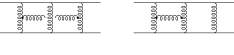
Figure 4: Graphs contributing to the three-loop IR divergence of the QCD static potential in perturbation theory.

ADM showed that this IR divergence could be avoided by summing diagrams with an arbitrary number of gluon rungs. This summation gives a factor $\exp([V_{s}(r)-V_{o}(r)]T)$ for the configuration space propagation of the intermediate color-octet $Q\bar{Q}$ pair, which regulates the IR divergence. In the pNRQCD framework the diagrams considered by ADM are obtained in the intermediate theory NRQCD, where the heavy quarks are treated in the static approximation. In Ref. [ $\!{}^{{\bf?}}$] Brambilla et al. made the important observation that, by construction, the ADM IR divergence is equivalent to IR divergences of (unresummed) pNRQCD graphs that describe the selfenergy of a quark-antiquark pair due to an ultrasoft gluon (see Fig. 5).

Figure 5: Selfenergy of a $Q\bar{Q}$ pair due to ultrasoft gluon radiation in pNRQCD.

Thus the static potential defined as the pNRQCD matching coefficient $\alpha_{V_{s}}$ is an infrared-safe quantity. As pointed out in Ref. [ $\!{}^{{\bf?}}$], this also means that the static potential defined via the Wilson loop

$$V_{\rm stat}(r)=\lim_{T\to\infty}{1\over T}\ln\left\langle{{\rm Tr}\,P\exp\Big{[}-ig\oint_{C}A_{\mu}dx^{\mu}\Big{]}}\right\rangle\,,$$ (37)

where $P$ refers to pathordering, is not equivalent to $V_{s}^{(0)}(r)$ at short distances, because the former contains the full ultrasoft selfenergy contributions just mentioned before.

The anomalous dimensions of the pNRQCD coefficients are determined from UV divergences in $Q\bar{Q}$ scattering diagrams, where again the $1/m$ expansion with off-shell static $Q\bar{Q}$ pairs at fixed distance $r$ (or with external momenta $(0,\pm\mathbf{p})$ and $(0,\pm\mathbf{p}^{\prime})$ for the incoming and outgoing quark) is used.$\!{}^{{\bf?},{\bf?}}$ At this stage, loop diagrams with UV divergences that occur in potential loop integration, i.e. when potential interactions are iterated, are neglected and only UV divergences from ultrasoft gluon exchange are considered.$\!{}^{{\bf?}}$ In particular, the iteration of static potential exchanges between the quarks is treated effectively in $D=4$ dimensions by using the resummed singlet/octet static $Q\bar{Q}$ propagator $\sim(-i\partial_{0}+V_{s,o}^{(0)}(r))^{-1}$, see Ref. [ $\!{}^{{\bf?}}$].

At leading order in the multipole expansion the entire ultrasoft renormalization of the potential coefficients is obtained from the effective one-loop selfenergy shown in Fig. 5, where the double line represents the static $Q\bar{Q}$ propagator. For example, the leading logarithmic (LL) running of the potentials $\propto 1/m^{2}$ is induced by the “one-loop” diagrams where the double line contains only one static potential exchange, see Fig. 6 for typical graphs.

Figure 6: Diagrams in pNRQCD that contribute to the anomalous dimension of the spin-independent $1/m^{2}$ potentials. The solid lines are static quark propagators. The dashed line represents the static potential.

At this level the LL expression for the coupling of the static potential is sufficient. Because the coupling of the static potential to the quarks does not run at LL order in pNRQCD, it is just $\alpha_{s}(\mu_{s})$. Due to gauge cancellations only the ${\mathbf{p}}.{\mathbf{A}}/m$ coupling of the ultrasoft gluons to quarks (which only runs trivially with $\alpha_{s}(\mu)$ at LL order) contributes and generically leads to the following LL anomalous dimension of the spin-independent $1/m^{2}$ coefficients,

$$\frac{d}{d\ln\mu}\Big{\{}\,D^{(2)}_{1,s}(\mu,\mu_{s}),D^{(2)}_{d,s}(\mu,\mu_{s})\,\Big{\}} \propto \alpha_{s}(\mu)\,\alpha_{s}(\mu_{s})\,.$$ (38)

At this order, the spin-dependent potentials do not run in pNRQCD.

A more involved example is the NNLL running of the static singlet potential $\alpha_{V_{s}}$, which was considered in Refs. [ $\!{}^{{\bf?},{\bf?}}$]. An ultrasoft anomalous dimension of $\alpha_{V_{s}}$ is generated for the first time by UV divergences in the “three-loop” diagrams in Fig. 7, which are also contained in the one-loop selfenergy of Fig. 5.

Figure 7: Diagrams in pNRQCD that contribute to the three-loop anomalous dimension of the static potential. The solid lines are static quark propagators. The static potential does not run at the one- and two-loop level.

The ultrasoft loop with the gluon propagator is UV-divergent. The two potential insertions are obtained by expanding the static $Q\bar{Q}$ propagator in terms of the static potential. At this order its coupling can again be approximated by $\alpha_{s}(\mu_{s})$. In momentum space the computation consists of an ultrasoft gluon loop in $D=4-2\epsilon$ dimensions, where the coupling of ultrasoft gluons to the static potential is $\alpha_{s}(\mu)$, and static quark loops in $D=4$ dimensions, where the couplings of the potentials to the quarks are $\alpha_{s}(\mu_{s})$. The incoming and outgoing quark momenta are $(0,\pm\mathbf{p})$ and $(0,\pm\mathbf{p}^{\prime})$, respectively. The ultrasoft loop is UV-divergent, and the static quark loops lead to the overall factor $1/(\mathbf{p}-\mathbf{p}^{\prime})^{2}$. For a color singlet $Q\bar{Q}$ pair the amplitude reads

Figs.7 $$= -i\frac{C_{F}\,C_{A}^{3}}{6}\,\frac{[\alpha_{s}(\mu_{s})]^{3}\,[\alpha_{s}(\mu)\,\mu^{2\epsilon}]}{(\mathbf{p}-\mathbf{p}^{\prime})^{2}}\bigg{[}\,\frac{1}{\epsilon_{\rm UV}}-\frac{1}{\epsilon_{\rm IR}}\,\bigg{]}\,.$$ (39)

The IR divergence $\propto 1/\epsilon_{\rm IR}$ is equivalent to the ADM infrared divergence mentioned above. The anomalous dimension for the static singlet potential obtained from the UV divergence reads

$$\frac{d}{d\ln\mu}\alpha_{V_{s}}(\mu,\mu_{s}) = \frac{C_{A}^{3}}{12\pi}\,[\alpha_{V_{s}}(\mu_{s})]^{3}\,\alpha_{s}(\mu)\,.$$ (40)

Using the initial condition of Eq. (36) the NNLL result for the static singlet potential at the scale $\mu=\mu_{u}$ reads $\!{}^{{\bf?}}$

$$\alpha_{V_{s}}(\mu_{u},\mu_{s}) = \Big{[}\alpha_{V_{s}}(\mu_{s})\Big{]}_{\mbox{\scriptsize two-loop}}+\bigg{[}\,\frac{C_{A}^{3}}{6\beta_{0}}\alpha_{s}^{3}(\mu_{s})\ln\bigg{(}\frac{\alpha_{s}(\mu_{s})}{\alpha_{s}(\mu_{u})}\bigg{)}\,\bigg{]}\,,$$ (41)

where $[\alpha_{V_{s}}(\mu_{s})]_{\mbox{\scriptsize two-loop}}$ is the two-loop matching result obtained from Eqs. (35) and (36).

4.4 Potential Loops in pNRQCD

If pNRQCD is applied to dynamical quarks, the counting $D_{0}\sim k^{0}\sim\frac{{{\mathbf{D}}}^{2}}{m}\sim\frac{{|{\mathbf{k}}|}^{2}}{2m}$ is reinstated and the potential region is reintroduced into the theory. As mentioned before, it is claimed in Refs. [ $\!{}^{{\bf?},{\bf?},{\bf?}}$] that the potential region is always contained in the pNRQCD framework, but hidden in a subtle way as long as the $1/m$ power counting is imposed. Potential loops, which are generated by iterations of potentials, can lead to UV divergences. Consider for example the $Q\bar{Q}$ scattering diagram in Fig. 8a with two $D_{d,s}^{(2)}$ potentials and one static potential. The $D_{d,s}^{(2)}$ potential is a $\delta$-function in configuration space, and the graph is UV divergent inducing a two-loop next-to-leading logarithmic (NLL) anomalous dimension to $D_{d,s}^{(2)}$. The diagram in Fig. 8b describes $Q\bar{Q}$ production and induces a two-loop NLL anomalous dimension to the coefficients of the $Q\bar{Q}$ production currents such as the ${}^{2s+1}L_{j}={}^{3}S_{1}$ current $O_{\psi\chi}=\psi^{\dagger}\mbox{\boldmath$\sigma$}(i\sigma_{2})\chi$.

Figure 8: Diagrams in pNRQCD that contribute to the two-loop anomalous dimension of the $D_{d,s}^{(2)}$ potential (a) and the $Q\bar{Q}$ production current (b).

Thus the LL running of $D_{d,s}^{(2)}$ and $\alpha_{V_{s}}$ obtained in NRQCD and from ultrasoft gluon radiation in pNRQCD mixes into $D_{d,s}^{(2)}$ and $c_{\psi\chi}$ at NLL order through UV divergences in potential loop diagrams. In order to quantify this mixing a correlation between the soft scale $\mu_{s}$, the ultrasoft scale $\mu_{u}$ and the scale for potential loops, $\mu_{p}$, needs to be imposed. Such a correlation does, by itself, not exist in the pNRQCD framework, since the quarks are treated as static. So the correlation needs to be imposed by hand, once potential loops and the counting $D_{0}\sim k^{0}\sim\frac{{{\mathbf{D}}}^{2}}{m}\sim\frac{{|{\mathbf{k}}|}^{2}}{2m}$ are reintroduced into the theory.

From the physical point of view this correlation should reflect the energy-momentum relation of the heavy quark: $\mu_{p}\sim\mu_{s}\sim\sqrt{\mu_{u}m}$. This concept has been first realized in the framework of vNRQCD, $\!{}^{{\bf?}}$ where the correlation of scales arises naturally from the theory itself. In Ref. [ $\!{}^{{\bf?}}$] Pineda proposed the following prescription for pNRQCD: after NRQCD is evolved to $\mu=\mu_{s}$ and the ultrasoft pNRQCD evolution is carried out down to the scale $\mu=\mu_{u}$ as described before, the relations

$$\mu_{s}\,=\,\mu_{p}\,,\quad\mu_{u}\,=\,\frac{\mu_{p}^{2}}{m}$$ (42)

are imposed. This scale correlation has to be used for the determination and the integration of the RGE’s obtained from potential UV divergences as well as for the determination of matrix elements, i.e. in particular in the solution of the Schrödinger equation. For the determination of all matrix elements the $1/m$ expansion is abandoned and the non-relativistic power counting from the regions in Eq. (21) is reestablished. For the integration of the renormalization group equations $\mu_{p}$ has to be run from the hard scale $m$ down to the soft scale of order $mv$. This procedure means in particular that, for the description of dynamical quarks, the end points of the running in NRQCD ($\mu_{s}$) and the ultrasoft running in pNRQCD ($\mu_{u}$) are generally not the soft and the ultrasoft scales of order $mv$ and $mv^{2}$, respectively. It is claimed in Ref. [ $\!{}^{{\bf?}}$] that this prescription sums properly all large logarithmic terms.

The NLL anomalous dimensions induced by Figs. 8a and b have the generic form

$$\frac{d}{\ln\mu_{p}}D_{d,s}^{(2)}\Big{(}\frac{\mu_{p}^{2}}{m},\mu_{p}\Big{)} \sim \bigg{[}D_{d,s}^{(2)}\Big{(}\frac{\mu_{p}^{2}}{m},\mu_{p}\Big{)}\bigg{]}^{2}\,\alpha_{V_{s}}\Big{(}\frac{\mu_{p}^{2}}{m},\mu_{p}\Big{)}\,,$$

$$\frac{d}{\ln\mu_{p}}c_{\psi\chi}(\mu_{p}) \sim c_{\psi\chi}(\mu_{p})\,D_{d,s}^{(2)}\Big{(}\frac{\mu_{p}^{2}}{m},\mu_{p}\Big{)}\,\alpha_{V_{s}}\Big{(}\frac{\mu_{p}^{2}}{m},\mu_{p}\Big{)}\,.$$ (43)

At this order, only the LL results need to be known on the RHS. The full NLL running of $D_{d,s}^{(2)}$ has actually not been calculated so far; it would be relevant for the description of the $Q\bar{Q}$ dynamics only at N³LL order. The NLL runnning of $c_{\psi\chi}$ in the pNRQCD framework has been determined in Ref. [ $\!{}^{{\bf?}}$].

4.5 Open Issues

There are issues in the pNRQCD framework that might require some investigations. One obvious point is that the matching procedures in the scheme of Eq. (28) appear to strongly rely on specific choices for the kinematic situation where the matching conditions can be calculated. It would be desirable that the matching procedure could be carried out for any kinematic situation, for which the effective theory is applicable. For example, the NRQCD matching is carried out for on-shell scattering amplitudes with external quarks exactly at the threshold point, where the quark velocity is zero. If on-shell scattering amplitudes with some small but non-zero quark velocity are employed the diagrams in full QCD also contain contributions from, let’s say, the potential momentum region, which cannot be reproduced in the $1/m$ expansion employed for the NRQCD computations.

Another issue concerns the prescription of Ref. [ $\!{}^{{\bf?}}$] for the treatment of UV divergences from potential loops after the endpoints of the NRQCD and ultrasoft pNRQCD running, $\mu_{s}$ and $\mu_{u}$, are correlated to the potential scale, $\mu_{p}=\mu_{s}=\sqrt{\mu_{u}m}$. The potentials that arise order-by-order from matching pNRQCD to NRQCD are independent of the matching scale $\mu_{s}$ up to higher order terms, which are small corrections in the matching conditions for $\mu_{s}\sim(\mathbf{p}-\mathbf{p}^{\prime})$, see for example Eq. (36) for the static potential. On the other hand, in the anomalous dimensions for $D_{d,s}^{(2)}$ and $c_{\psi\chi}$ in Eqs. (43) the residual dependence of for example $\alpha_{V_{s}}$ on $\mu_{s}$ leads to the summation of unphysical logarithms unless the corresponding logarithmic terms in the matching computation for the potential are summed too. This means in principle that the higher order matching corrections to the potentials cannot be considered as small when correlated running according to Ref. [ $\!{}^{{\bf?}}$] is employed.

It is a prediction of the pNRQCD framework that the Coulomb potential in the Schrödinger equation that describes dynamical $Q\bar{Q}$ pairs is equal to the static potential determined in the $1/m$ expansion in pNRQCD.$\!{}^{{\bf?}}$ The ultrasoft anomalous dimension of the static potential is determined from Eq. (39), which does not contain any scale dependence from the static ladder diagrams that iterate the potentials. On the other hand, after the scale correlation $\mu_{p}=\mu_{s}=\sqrt{\mu_{u}m}$ and the non-relativistic power counting are imposed, the corresponding UV divergent contribution from the diagram in the N³LL matrix element describing let’s say on-shell $Q\bar{Q}$ scattering in analogy to Fig. 7 reads

$$i\frac{C_{F}\,C_{A}^{3}}{6}\,\frac{[\alpha_{s}(\mu_{s})\,\mu_{s}^{2\epsilon}]^{3}\,[\alpha_{s}(\mu_{u})\,\mu_{u}^{2\epsilon}]}{(\mathbf{p}-\mathbf{p}^{\prime})^{2}}\bigg{[}\,\frac{1}{\epsilon}\,\bigg{]}\,,$$ (44)

where the dependence on $\mu_{s}$ and $\mu_{u}$ has been made manifest. Here, the scale dependence of the potential loops is included, because the quarks are not static. The $1/\epsilon$ term is canceled by the counterterm of the Coulomb potential determined from Eq. (39). However, only a part of the $\ln\mu_{p}$ terms is canceled by the order $\alpha_{s}^{4}$ ultrasoft logarithm summed into $\alpha_{V_{s}}$ by Eq. (40). The remaining $\ln\mu_{p}$ terms seem to remain uncanceled in the final N³LL result for $Q\bar{Q}$ scattering.

4.6 $\Lambda_{\rm QCD}\sim mv^{2}$ or larger

So far pNRQCD has been discussed for the case $m\gg mv\gg mv^{2}\gg\Lambda_{\rm QCD}$, where the counting $\alpha_{s}(m)\sim\alpha_{s}(mv)\sim\alpha_{s}(mv^{2})\ll 1$ was used. In this situation the description of the $Q\bar{Q}$ dynamics is predominantly perturbative and the effective theories serve mainly as a tool to handle the non-trivial perturbative calculations and summations in a manageable and systematic fashion. Non-perturbative effects appear as local gluon and light quark condensates in an expansion in $\Lambda_{\rm QCD}/mv^{2}$, see Refs. [ $\!{}^{{\bf?},{\bf?},{\bf?}}$]. One motivation in the construction of pNRQCD was that its multi-layer structure should make it also applicable to systems where $\Lambda_{\rm QCD}$ is of order $mv^{2}$ or larger. In this case also the non-relativistic dynamics of the charmonium or of higher bottomonium excitations could be studied in a systematic and quantitative manner. Qualitative discussions of the application of pNRQCD in cases where $\Lambda_{\rm QCD}$ is of order $mv^{2}$ or larger have been given in Ref. [ $\!{}^{{\bf?}}$]. For $mv>\Lambda_{\rm QCD}\mathrel{\raise 1.29167pt\hbox{$>$\kern-7.5pt\lower 4.30554pt\hbox{$\sim$}}}mv^{2}$ pNRQCD can still be matched perturbatively to NRQCD at the soft scale $\mu_{s}$, but $\Lambda_{\rm QCD}$ screens the ultrasoft scale (or any other lower scale) and $\alpha_{s}(mv^{2})$ is of order $1$. However, the coupling of ultrasoft ($\sim\Lambda_{\rm QCD}$) gluons to the quark-antiquark pair $\propto{\mathbf{r}}.{\mathbf{E}}$ is still small because of the multipole expansion. The effects of ultrasoft gluons enter as non-perturbative non-local condensates, that are small corrections. For $\Lambda_{\rm QCD}\mathrel{\raise 1.29167pt\hbox{$>$\kern-7.5pt\lower 4.30554pt\hbox{$\sim$}}}mv$, the matching of NRQCD to QCD at the hard scale can still be carried out perturbatively, but the full non-relativistic $Q\bar{Q}$ dynamics is screened by $\Lambda_{\rm QCD}$. In this case NRQCD (Sec. 2) should describe $Q\bar{Q}$ production and decay, but all non-relativistic $Q\bar{Q}$ dynamics is non-perturbative.

5 Effective Theories III: Velocity NRQCD

The effective theory vNRQCD was first proposed by Luke, Manohar and Rothstein.$\!{}^{{\bf?}}$ It is devised for systems where the relation $m\gg mv\gg mv^{2}\gg\Lambda_{\rm QCD}$ is valid. Its main fields of application are top pair production close to threshold, sum rules for $\Upsilon$ mesons and maybe low radial excitations of bottomonia. The theory vNRQCD provides the separation of all different degrees of freedom in a single step at the hard scale and is defined in dimensional regularization.

5.1 Basic Idea

The basic idea behind the construction of vNRQCD is that all resonant degrees of freedom (dof’s) (i.e. dof’s that can develop a particle pole in the momentum regions of Eq. (21)) are separated and that all off-shell fluctuations (i.e. fluctuations that cannot come close to their mass-shell in the regions of Eq. (21)) are integrated out at the hard scale. This means that the theory contains different gluon field operators for the gluonic fluctuations with soft and ultrasoft energies and momenta. The theory vNRQCD is matched to QCD at the scale $m$ and the renormalization group equations are constructed such that large logarithms of the scale ratios $m/\langle p\rangle$, $m/\langle E\rangle$ and $\langle p\rangle/\langle E\rangle$ are summed simultaneously into the coefficients of the operators when the theory is scaled down. This is achieved by having different renormalization scales for potential/soft and ultrasoft loop integrals, which are correlated in accordance with the quark equations of motion. The scale correlation is fixed by the theory itself and not imposed by hand. The correlation of the scales and the renormalization group evolution are expressed in terms of the “velocity” scaling parameter $\nu$. The hard scale corresponds to $\nu=1$ and all large logarithmic terms are summed for $\nu=v$.

5.2 Effective Lagrangian

The effective Lagrangian is formulated in terms of quark and gluonic fields describing modes that can become on-shell in the momentum regions of Eq. (21). For convenience, massless quarks will be referred to as gluons in the following presentation. Heavy quarks are simply referred to as quarks. On-shell fluctuations for quarks exist only for the potential regime where $(k_{0},{\mathbf{k}})\sim(mv^{2},mv)$ and on-shell gluonic fluctuations exist in the soft and the ultrasoft regime where $(k_{0},{\mathbf{k}})\sim(mv,mv)$ and $(k_{0},{\mathbf{k}})\sim(mv^{2},mv^{2})$, respectively. These three kinds of modes are referred to as “potential quarks”, “soft gluons” and “ultrasoft gluons”. Although soft gluons cannot be produced in a non-relativistic $Q\bar{Q}$ system with total energy of the order $mv^{2}$, they are kept as relevant dof’s in vNRQCD. This is necessary because interactions with soft gluons are involved in the renormalization of vNRQCD operators. In fact, one can consider vNRQCD as a theory that can describe interactions of a quark with soft gluons as well, such as in Compton scattering.

In the effective Lagrangian only ultrasoft energies and momenta are treated as continuous variables. Soft energies and momenta are treated as discrete indices for potential quarks and soft gluons. For a heavy quark this is achieved by writing its energy $E$ and three-momentum $\mathbf{P}$ as

$$E\,=\,k^{0}\,,\qquad\mathbf{P}\,=\,\mathbf{p}+\mathbf{k}$$ (45)

where the three-vector $\mathbf{p}$ is of order of the soft scale $mv$ and the four-vector $k=(k^{0},\mathbf{k})$ is of order of the ultrasoft scale $mv^{2}$. This can be understood as subdividing the full non-relativistic momentum space for the quark three-momentum (with side length of order $mv$) into small cubes with ultrasoft side length of order $mv^{2}$, such that the number of ultrasoft cubes is $(\frac{mv}{mv^{2}})^{3}$. The center location of each ultrasoft cube is given by the index $\mathbf{p}$ and a point within an ultrasoft cube is labeled by $\mathbf{k}$, see Fig. 9.

Figure 9: Momentum space of size $mv$ is divided into boxes of size $mv^{2}$. A point in momentum space is labeled by $\mathbf{p}$ and $\mathbf{k}$.

Only the ultrasoft four-momenta $k$ are treated as continuous variables, the soft three-momentum $\mathbf{p}$ is a discrete index. The number soft three-momenta is equal to the number of ultrasoft cubes. The quark and antiquark fields in vNRQCD are written as two-component spinor fields

$$\psi_{\mathbf{p}}(x)\,,\quad\chi_{\mathbf{p}}(x)\,,$$ (46)

where $\mathbf{p}$ is the soft index and $x$ the continuous variable that describes ultrasoft fluctuations. This procedure is similar to HQET, $\!{}^{{\bf?}}$ where the four-momentum $q^{\mu}$ of a heavy quark is split into $mv^{\mu}$ of order $m$ and a residual four-momentum $k$ of order $\Lambda_{\rm QCD}$, $q^{\mu}=mv^{\mu}+k^{\mu}$. The index $v^{\mu}$ is a discrete variable one has to sum, whereas $k^{\mu}$ is a continuous variable one has to integrate. In vNRQCD one has to sum over $\mathbf{p}$ and integrate over $x$ (or $k$ in momentum space representation).

The energy $E$ and three-momentum $\mathbf{P}$ of a soft gluon is written in an analogous way as

$$E\,=\,p^{0}+k^{0}\,,\qquad\mathbf{P}\,=\,\mathbf{p}+\mathbf{k}\,,$$ (47)

where $p=(p_{0},\mathbf{p})$ is a four-vector of the order of the soft scale $mv$ and $k=(k_{0},\mathbf{k})$ is a four-vector of the order of the ultrasoft scale $mv^{2}$. The corresponding field in vNRQCD that annihilates and creates a soft gluon with index $p$ in vNRQCD is $A_{p}^{\mu}(x)$. One has to sum over $p$ and integrate over $x$ (or $k$). The energy $E$ and the three-momentum $P$ of an ultrasoft gluon is just

$$E\,=k^{0}\,,\qquad\mathbf{P}\,=\mathbf{k}\,,$$ (48)

where $k=(k_{0},\mathbf{k})$ is a four-vector of the order of the ultrasoft scale $mv^{2}$. The corresponding field in vNRQCD that annihilates and creates an ultrasoft gluon vNRQCD is $A^{\mu}(x)$.

The decomposition into a soft and an ultrasoft momentum component of let’s say the quark is not unique. Taking an ultrasoft three-momentum $\mathbf{q}$ one can redefine

$$\mathbf{k}\to\mathbf{k}+\mathbf{q}\,,\qquad\mathbf{p}\to\mathbf{p}-\mathbf{q}\,.$$ (49)

This reparametrization invariance is similar to HQET,$\!{}^{{\bf?}}$ but it does not affect the spin axis of the quarks, because the latter is fixed by the choice of the center of mass frame, which is not affected by the transformation in Eq. (49). So the consequences of reparametrization invariance in vNRQCD are the same as for HQET for spin-zero particles. The basic outcome of reparametrization invariance in vNRQCD is that derivatives of $\psi_{\mathbf{p}}(x)$ or $\chi_{\mathbf{p}}(x)$ are always of the form $(i\mathbf{p}+\mathbf{\nabla})$.

The effective Lagrangian is written in terms of quark fields, $\psi_{\mathbf{p}}$, antiquark fields, $\chi_{\mathbf{p}}$, soft gluon fields, $A_{\mathbf{q}}^{\mu}$, and an ultrasoft gluon field, $A^{\mu}$. The covariant derivative is $D^{\mu}=(D^{0},{\mathbf{D}})$ with $D^{0}=\partial^{0}+igA^{0}$, ${\mathbf{D}}={\mathbf{\nabla}}-ig{\mathbf{A}}$, and it involves only the ultrasoft gluon field. The effective Lagrangian is manifestly gauge-invariant with respect to ultrasoft gauge transformations, i.e. with slowly varying gauge phases involving frequencies of order $mv^{2}$. It is argued in Ref. [ $\!{}^{{\bf?}}$] that the full gauge invariance including also higher frequencies of order $mv$ is recovered by combination of reparametrization invariance and ultrasoft gauge invariance. A mathematical proof of this conjecture does, however, not yet exist.

In the center of mass frame the Lagrangian has the form $\!{}^{{\bf?},{\bf?},{\bf?}}$

$${\cal L}_{\rm vNRQCD}\,=\,\sum_{\mathbf{p}}\,\bigg{\{}\psi_{\mathbf{p}}^{\dagger}\bigg{[}iD^{0}-{\left({\bf p}-i{\bf D}\right)^{2}\over 2m}+\frac{{\mathbf{p}}^{4}}{8m^{3}}+\ldots\bigg{]}\psi_{\mathbf{p}}+(\psi\to\chi)\,\bigg{\}}\quad\mbox{}$$ (50)

$$-g^{2}\sum_{{\mathbf{p}},{\mathbf{p}^{\prime}},q,q^{\prime},\sigma}\bigg{\{}\frac{1}{2}\,\psi_{\mathbf{p}^{\prime}}^{\dagger}[A^{\mu}_{q^{\prime}},A^{\nu}_{q}]U_{\mu\nu}^{(\sigma)}\psi_{\mathbf{p}}+(\psi\to\chi)+\ldots\,\bigg{\}}$$

$$+\frac{2ig^{2}}{(\mathbf{p}^{\prime}-\mathbf{p})^{4}}f^{ABC}{(\mathbf{p}-\mathbf{p}^{\prime})}.(g{\mathbf{A}}^{C})[\psi_{\mathbf{p}^{\prime}}^{\dagger}T^{A}\psi_{\mathbf{p}}\chi_{-\mathbf{p}^{\prime}}^{\dagger}\bar{T}^{B}\chi_{-\mathbf{p}}]+\ldots\qquad\quad\mbox{}$$

$$-\,V({\mathbf{p},\mathbf{p}^{\prime}})\,\psi_{\mathbf{p}^{\prime}}^{\dagger}\psi_{\mathbf{p}}\chi_{-\mathbf{p}^{\prime}}^{\dagger}\chi_{-\mathbf{p}}$$

$$-{1\over 4}G^{\mu\nu}G_{\mu\nu}+\sum_{p}\left|p^{\mu}A^{\nu}_{p}-p^{\nu}A^{\mu}_{p}\right|^{2}+\ldots\,,$$

where ($\mathbf{k}=(\mathbf{p}-\mathbf{p}^{\prime})$)

$$V({\mathbf{p}},{\mathbf{p}^{\prime}})\,=\,(T^{A}\otimes\bar{T}^{A})\bigg{[}\frac{{\cal V}_{c}^{(T)}}{\mathbf{k}^{2}}+\frac{{\cal V}_{k}^{(T)}\pi^{2}}{m|{\mathbf{k}}|}+\frac{{\cal V}_{r}^{(T)}({\mathbf{p}^{2}+\mathbf{p}^{\prime 2}})}{2m^{2}\mathbf{k}^{2}}+\frac{{\cal V}_{2}^{(T)}}{m^{2}}+\frac{{\cal V}_{s}^{(T)}}{m^{2}}{\mathbf{S}^{2}}$$

$$+\,\frac{{\cal V}_{\Lambda}^{(T)}}{m^{2}}\Lambda({\mathbf{p}^{\prime},\mathbf{p}})+\frac{{\cal V}_{t}^{(T)}}{m^{2}}\,T({\mathbf{k}})\bigg{]}+(1\otimes 1)\bigg{[}\frac{{\cal V}_{k}^{(1)}\pi^{2}}{m|{\mathbf{k}}|}+\frac{{\cal V}_{2}^{(1)}}{m^{2}}+\frac{{\cal V}_{s}^{(1)}}{m^{2}}{\mathbf{S}^{2}}\bigg{]}\,,\qquad\quad$$

$${\mathbf{S}}\,=\,{{{\mathbf{\mbox{\boldmath$\sigma$}}}_{1}+{\mathbf{\mbox{\boldmath$\sigma$}}}_{2}}\over 2}\,,\qquad\Lambda({\mathbf{p}^{\prime}},{\mathbf{p}})\,=\,-i{{\mathbf{S}}\cdot({\mathbf{p}^{\prime}}\times{\mathbf{p}})\over{\mathbf{k}}^{2}}\,,$$

$$T({\mathbf{k}})\,=\,{{\mathbf{\mbox{\boldmath$\sigma$}}}_{1}\cdot{\mathbf{\mbox{\boldmath$\sigma$}}}_{2}}-{3\,{{\mathbf{k}}\cdot{\mathbf{\mbox{\boldmath$\sigma$}}}_{1}}\,{{\mathbf{k}}\cdot{\mathbf{\mbox{\boldmath$\sigma$}}}_{2}}\over{\mathbf{k}}^{2}}\,,$$ (51)

and

$$U^{(0)}_{00} = \frac{1}{q^{0}}\,,\quad U^{(0)}_{0i}=-\frac{{({2\mathbf{p}^{\prime}}-2{\mathbf{p}}-{\mathbf{q}})}^{i}}{({\mathbf{p}}-{\mathbf{p}}^{\prime})^{2}}\,,$$

$$U^{(0)}_{i0} = -\frac{({\mathbf{p}}-{\mathbf{p}}^{\prime}-{\mathbf{q}})^{i}}{({\mathbf{p}}-{\mathbf{p}}^{\prime})^{2}}\,,\quad U^{(0)}_{ij}=\frac{-2q^{0}\delta^{ij}}{({\mathbf{p}}-{\mathbf{p}}^{\prime})^{2}}\,.$$ (52)

The matrices $T^{A}$ and $\bar{T}^{A}$ are the color matrices for the $\bf 3$ and $\bf\bar{3}$ representations, $igG^{\mu\nu}=\left[D^{\mu},D^{\nu}\right]$ and $m$ is the heavy quark pole mass. Interactions involving ghosts and light quarks are not displayed. The effective Lagrangian (second line) contains interactions between quarks and soft gluons. Due to energy conservation at least two soft gluons participate in interactions with quarks. Graphically the interaction of a quark with two soft gluons is represented by Fig. 10d.

Figure 10: The Compton scattering diagrams (a,b,c) in full QCD generate the soft gluon coupling (d) in vNRQCD. Soft gluon modes are denoted by a zigzag line

The explicit form of the leading order soft interactions is displayed in Eq. (52). The $1/q^{0}$ term that is visible for example in $U_{00}^{(0)}$ arises from the propagation of an off-shell “soft quark”, see Fig. 10. The term does not have an $i\delta$ prescription and does not lead to poles or pinch-singularities when the loop integral over $q_{0}$ is carried out by contours. Terms in the expansion of full QCD such as

$$\frac{1}{k_{0}+i\delta}-\frac{1}{k_{0}-i\delta}$$

lead to additional four-quark interactions with soft gluons in the matching procedure.$\!{}^{{\bf?},{\bf?}}$ There are terms in the Lagrangian where ultrasoft gluons couple to potential operators. The term in the third line of Eq. (50) for example is generated by a QCD diagram similar to the third diagram in Fig. 3. There are potential-type four-quark interactions (fourth line) that depend non-locally on the soft indices, but are local interactions with respect to the dynamical ultrasoft fluctuations. They are graphically represented by Fig. 11b.

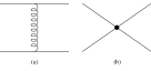
Figure 11: The scattering Born diagram (a) generates the potential four-quark interaction (b) in vNRQCD.

In Eq. (51) the leading order Coulomb potential interaction and the $v$- and $v^{2}$-suppressed potentials are displayed. The basis in terms of $(1\otimes 1)$ and $(T^{A}\otimes\bar{T}^{A})$ can be converted to the color singlet and octet basis by the transformation

$$\left[\begin{array}[]{c}V_{\rm singlet}\cr V_{\rm octet}\end{array}\right]=\left[\begin{array}[]{ccc}1&&-C_{F}\cr 1&&{1\over 2}C_{A}-C_{F}\cr\end{array}\right]\left[\begin{array}[]{c}V_{1\otimes 1}\cr V_{T\otimes T}\end{array}\right]\,.$$ (59)

The multipole expansion has to be applied strictly for all terms in the effective Lagrangian in order to achieve separation of the modes in the different regions. For example the term $({\mathbf{p}}-i{\mathbf{D}})^{2}$ in the bilinear quark sector has to be considered as an expansion in $\mathbf{D}$ because $i\mathbf{D}\ll\mathbf{p}$. Interactions between soft and ultrasoft gluons without (heavy) quarks do not exist because ultrasoft modes cannot resolve the “high frequency” soft gauge transformations (that are realized through reparametrization invariance). On the other hand, the soft gauge fields feel ultrasoft gauge transformations just as a global phase transformation.$\!{}^{{\bf?}}$

The velocity power counting of the fields can be derived from demanding that the action for the kinetic terms is of order $v^{0}$ and reads

$$\mathbf{p} \psi_{\mathbf{p}},\ \chi_{\mathbf{p}} A_{p}^{\mu} D^{0} \mathbf{D} A^{\mu} v v^{3/2} v v^{2} v^{2} v^{2}$$ . (60)

Soft and ultrasoft massless quark fields count as $v^{3/2}$ and $v^{3}$, respectively.

External currents describing quark production, annihilation or decay are also built from the quark fields in Eq. (46). For example, consider $Q\bar{Q}$ production at NNLL order in $e^{+}e^{-}$ annihilation. One needs the ${}^{3}S_{1}$ (vector) current with dimension three and five,

$$\mbox{\boldmath$O$}_{\mbox{\scriptsize$\mathbf{p}$},1} = {\psi_{\mathbf{p}}}^{\dagger}\,\mbox{\boldmath$\sigma$}(i\sigma_{2})\,{\chi_{\mathbf{-p}}^{*}}\,,$$

$$\mbox{\boldmath$O$}_{\mbox{\scriptsize$\mathbf{p}$},2} = \frac{1}{m^{2}}\,{\psi_{\mathbf{p}}}^{\dagger}\,{\mathbf{p}}^{2}\mbox{\boldmath$\sigma$}(i\sigma_{2})\,{\chi_{\mathbf{-p}}^{*}}\,,$$ (61)

and the ${}^{3}P_{1}$ (axial-vector) current with dimension four

$$\mbox{\boldmath$O$}_{\mbox{\scriptsize$\mathbf{p}$},3} = \frac{-i}{2m}\,{\psi_{\mathbf{p}}}^{\dagger}\,[\,\mbox{\boldmath$\sigma$},\mbox{\boldmath$\sigma$}\cdot{\mathbf{p}}\,]\,(i\sigma_{2})\,{\chi_{\mathbf{-p}}^{*}}\,.$$ (62)

The currents describe production of a $Q\bar{Q}$ pair with momentum $\pm\mathbf{p}$. The corresponding annihilation currents $\mbox{\boldmath$O$}_{\mbox{\scriptsize$\mathbf{p}$},1-3}^{\dagger}$ are obtained from complex conjugation.

5.3 Loops and Correlation of Scales

A general multi-loop graph in vNRQCD is divided into soft, potential and ultrasoft loop subgraphs. The diagram in Fig. 12a shows a typical ultrasoft loop.

                       

Figure 12: Typical one-loop diagrams in vNRQCD containing ultrasoft (a), potential (b) and soft (c) loop integrals.

Because an ultrasoft gluon cannot change the soft index of a quark the loop does not involve any sum over soft indices of the quark. In dimensional regularization the integration measure of the ultrasoft loop reads ($D=4-2\epsilon$)

$$\mu_{U}^{4-D}\int\frac{d^{D}k}{(2\pi)^{D}}\,,$$ (63)

where $\mu_{U}$ is the common renormalization scale for the ultrasoft dynamical fluctuations introduced to keep couplings dimension-less. In vNRQCD $\mu_{U}$ is rewritten as

$$\mu_{U}\,\equiv\,m\nu^{2}\,,$$ (64)

where $\nu$ is called the “velocity scaling parameter” and $\nu=1$ corresponds to $\mu_{U}=m$. The reason for introducing $\nu$ will become clear below. The natural choice for the velocity scaling parameter in matrix elements is $\nu\approx v$. The integral for the ultrasoft loop is carried out over the full $D$-dimensional non-relativistic space. The information that the loop is dominated by the ultrasoft region is implemented by the pole structure of the propagators and the multipole expansion.

In Fig. 12b a typical potential loop diagram is displayed. Its integration measure reads

$$\mu_{U}^{4-D}\sum\limits_{\mathbf{p}}\int\frac{d^{D}k}{(2\pi)^{D}}$$ (65)

and involves an integral over an ultrasoft momentum and a sum over all possible soft indices of intermediate quark-antiquark pairs. In practical analytical calculations it is convenient to rewrite the combination of the sum and the ultrasoft integration as an integral over the full $D$-dimensional non-relativistic momentum space. The number of terms in the sum is $(\frac{\mu_{S}}{\mu_{U}})^{3}$, where

$$\mu_{S}\,\equiv\,m\nu\,.$$ (66)

Thus Eq. (65) can be written as

$$\bigg{[}\,\mu_{U}^{4-D}\Big{(}\frac{\mu_{S}}{\mu_{U}}\Big{)}^{3}\Big{(}\frac{\mu_{S}}{\mu_{U}}\Big{)}^{1-D}\,\bigg{]}\,\sum\limits_{\mathbf{p}}^{D\mbox{\scriptsize-dim.}}\int\frac{d^{D}k}{(2\pi)^{D}}\,=\,\mu_{S}^{4-D}\int\frac{d^{D}p}{(2\pi)^{D}}\,,$$ (67)

and we find that vNRQCD itself “recognizes” that the proper renormalization scale for a potential loop is the soft scale $\mu_{S}$. The pole structure of the propagators and the multipole expansion determine that the loop is dominated by the potential region. For a typical soft loop such as in Fig. 12c the same renormalization scale $\mu_{S}$ arises, when the combination of sum and ultrasoft integration is written as an integral over the full $D$-dimensional non-relativistic momentum space,

$$\mu_{U}^{4-D}\sum\limits_{q}\int\frac{d^{D}k}{(2\pi)^{D}}\,\to\,\mu_{S}^{4-D}\int\frac{d^{D}q}{(2\pi)^{D}}\,.$$ (68)

The pole structure of the propagators and the multipole expansion determine that the loop is dominated by the soft region. For more complicated multi-loop diagrams the same rules apply. Soft and potential loops have the renormalization scale $\mu_{S}$ and purely ultrasoft loops the renormalization scale $\mu_{U}$. Whether a loop is either soft, potential or ultrasoft is determined by the pole structure of the propagators and the multipole expansion.

In vNRQCD there are two renormalization scales, which are correlated such that a “subtraction velocity” $\nu$ can be defined. The parameter $\nu$ serves as the natural scaling parameter for all types of loop integrals in vNRQCD. The scale correlation is not imposed by hand, but an intrinsic property of the theory itself. The physical origin of the correlation $\mu_{U}=\frac{\mu_{S}^{2}}{m}$ is the equation of motion of the quark, which relates the soft and ultrasoft energy scales. The renormalization scales can be naturally incorporated in the effective Lagrangian in $D=4-2\epsilon$ dimensions to keep the couplings dimensionless.$\!{}^{{\bf?}}$ In general, a vertex with $2+i$ quarks, $j$ soft gluons and $k$ ultrasoft gluons receives a factor $[\mu_{S}^{(i+j)\epsilon}\,\mu_{U}^{k\epsilon}]$.

Without the correlation of scales vNRQCD becomes inconsistent. Consider, for example, the three-loop diagram in Fig. 13a, which contributes to the renormalization of the dimension-three ${}^{3}S_{1}$ $Q\bar{Q}$ current ${\cal O}_{\mathbf{p},1}=\psi_{\mathbf{p}}^{\dagger}\mbox{\boldmath$\sigma$}(i\sigma_{2})\chi_{-\mathbf{p}}^{*}$.

Figure 13: Examples of graphs that contribute to the three-loop anomalous dimension for $c_{1}$. $\delta{\cal V}_{2,r}$ are one loop counterterms. The coupling of the ultrasoft gluon to the quarks is $g{\mathbf{p}}.{\mathbf{A}}/m$, where the scale of g is $m\nu^{2}$.

The operator ${\cal O}_{\mathbf{p},1}$ describes for example the leading order production of $Q\bar{Q}$ pairs in $e^{+}e^{-}$ annihilation. After subtraction of all UV subdivergences for $\epsilon\to 0$ through the diagrams in Fig. 13b the remaining overall UV divergence leads to the following counter term contribution for the coefficient $c_{1}$ of the operator ${\cal O}_{\mathbf{p},1}$,

$$\delta c_{1}\,\sim\,\alpha_{s}(m\nu^{2})\,[{\cal V}_{c}^{(T)}(\nu)]^{2}\bigg{[}\,\frac{\#}{\epsilon^{2}}+\frac{\#}{\epsilon}\,\Big{(}\,\ln\mu_{U}-2\ln\mu_{S}+\#\,\Big{)}\,\bigg{]}\,,$$ (69)

where $\#$ symbolizes real numbers. The anomalous dimension for $c_{1}$ can be determined unambiguously only if the correlation between $\mu_{U}$ and $\mu_{S}$ is accounted for.$\!{}^{{\bf?}}$

The computation of matching conditions and anomalous dimensions proceeds in the canonical way taking the velocity scaling parameter $\nu$ as the fundamental renormalization scaling variable in dimensional regularization. This is the origin of the “v” in vNRQCD.

5.4 Power Counting

The velocity power counting can be carried out using the velocity scaling rules of energies and momenta in the soft, potential and ultrasoft regions of Eq. (21). At this point the power counting is similar to the one in the threshold expansion and relies on assigning powers of $v$ to all loop measures, propagators and vertices in vNRQCD diagrams. An equivalent but more convenient power counting prescription has been derived in Ref. [ $\!{}^{{\bf?}}$]. It relies only on $v$-counting for the vertices of the effective Lagrangian and the topology of the soft momentum component in loop diagrams. Let $V_{k}^{(S)}$, $V_{k}^{(U)}$ and $V_{k}^{(P)}$ denote the number of soft, ultrasoft and potential vertices of order $v^{k}$ in a given graph, where the velocity counting of the fields in Eq. (60) is included. Here, ultrasoft vertices involve only ultrasoft fields, potential vertices involve at least one quark and no soft fields, and soft vertices at least one soft field. For example, the vertices

$$\psi_{\mathbf{p}}^{\dagger}\frac{{\mathbf{p}}.{\mathbf{D}}}{m}\psi_{\mathbf{p}}\,,\quad\psi_{\mathbf{p}^{\prime}}^{\dagger}\frac{1}{q^{0}}[A_{q^{\prime}},A_{q}]\psi_{\mathbf{p}}\,,\quad{\rm and}\quad\psi_{\mathbf{p}^{\prime}}^{\dagger}\psi_{\mathbf{p}}\frac{1}{(\mathbf{p}-\mathbf{p}^{\prime})^{2}}\chi_{-\mathbf{p}^{\prime}}^{\dagger}\chi_{-\mathbf{p}}$$

have $V_{6}^{(P)}$, $V_{4}^{(S)}$ and $V_{4}^{(P)}$, respectively. The ultrasoft gauge kinetic term $G^{\mu\nu}G_{\mu\nu}$ has $V_{8}^{(U)}$. For soft and potential vertices vertices $k\geq 4$ and for ultrasoft vertices $k\geq 8$. A given diagram is then of order $v^{\delta}$, where $\!{}^{{\bf?}}$

$$\delta\,=\,5+\sum_{k}\left[(k-8)V^{(U)}_{k}+(k-5)V^{(P)}_{k}+(k-4)V^{(S)}_{k}\right]-N_{S}\,,$$ (70)

$N_{S}$ being the number of connected soft components of the diagram. Ultrasoft and soft vertices can only give positive contributions to the sum. Potential vertices give positive contributions except for the Coulomb potential interaction, which has $V_{4}^{(P)}$. An insertion of $n$ Coulomb potentials lowers $\delta$ by $n$, but leaves the $v$-counting unchanged if one also counts the Coulomb coupling as ${\cal V}_{c}\sim\alpha_{s}\sim v$. Thus each additional insertion of a Coulomb potential gives a factor $\alpha_{s}v^{-1}$. It is therefore convenient to count the Coulomb potential $\propto\alpha_{s}/{\mathbf{k}}^{2}$ simply as of order $\alpha_{s}v^{-1}$, the $1/m|{\mathbf{k}}|$ potentials as of order $\alpha_{s}v^{0}$ and the $1/m^{2}$ potentials as of order $\alpha_{s}v^{1}$, etc..

For illustration let us consider the graph displayed in Fig. 14, which has $V_{6}^{(P)}=2$ and $V_{4}^{(P)}=2$. Thus one obtains $\delta=5+(6-5)\times 2+(4-5)\times 2=5$, so the graph is of order $\alpha_{s}^{3}\,v^{5}$.

Figure 14: Examples of graph or order $\alpha_{s}^{3}\,v^{5}$. The coupling of the ultrasoft gluon to the quarks is $g{\mathbf{p}}.{\mathbf{A}}/m$.

Dividing this result by the velocity counting of the four external quark fields ($v^{6}$), we find that the amputated graph is of order $\alpha_{s}^{3}\,v^{-1}$. The same result is found from the $v$-counting of the loop measures, propagators and vertices based on the velocity scaling of the ultrasoft and potential regions in Eq. (21). The diagram in Fig. 14 is suppressed by $\alpha_{s}\,v^{2}$ with respect to the same graph without the ultrasoft gluon, which is of order $\alpha_{s}^{2}v^{3}$. Each additional ultrasoft gluon gives an additional factor $\alpha_{s}v^{2}$. If we apply the same counting rules to QED we find that the Lamb-shift, which is caused by ultrasoft photons, is suppressed by a factor $\alpha v^{2}\sim\alpha^{3}$ with respect to the leading Coulomb interaction.

5.5 Matching

The determination of the matching conditions of the coefficients in the effective Lagrangian at the hard scale, $\nu=1$, is carried out with amplitudes for on-shell quarks and gluons. This avoids operators that vanish by the equation of motion and gauge-dependent matching conditions. Any kinematic situation described by the effective theory can be used for the matching calculation. For example, at the Born level the matching conditions for the potentials obtained from the on-shell graphs in Fig. 11 are $\!{}^{{\bf?}}$

$${\cal V}_{c}^{(T)}(1) = 4\pi\alpha_{s}(m)\,,\qquad{\cal V}_{r}^{(T)}(1)=4\pi\alpha_{s}(m)\,,\qquad{\cal V}_{s}^{(T)}(1)=-\frac{4\pi\alpha_{s}(m)}{3}\,,$$

$${\cal V}_{\Lambda}^{(T)}(1) = -6\pi\alpha_{s}(m)\,,\qquad{\cal V}_{t}^{(T)}(1)=-\frac{\pi\alpha_{s}(m)}{3}\,.\qquad$$ (71)

Matching conditions that vanish and annihilation contributions are not shown in Eq. (71). The on-shell matching conditions for the potentials at the one-loop level were computed in Ref. [ $\!{}^{{\bf?}}$]. For the order $1/(m\mathbf{k})$ potentials the results read

$${\cal V}_{k}^{(T)}(1) = \alpha_{s}^{2}(m)\Big{(}\frac{7C_{A}}{8}-\frac{C_{d}}{8}\Big{)}\,,\qquad{\cal V}_{k}^{(1)}(1)=\alpha_{s}^{2}(m)\frac{C_{1}}{2}\,,$$ (72)

where $C_{d}=8C_{F}-3C_{A}$ and $C_{1}=C_{F}(\frac{1}{2}C_{A}-C_{F})$. For SU$(N)$ we have

$$C_{F}=\frac{N^{2}-1}{2N}\,,\quad C_{A}=N\,,\quad C_{d}=\frac{N^{2}-4}{N}\,,\quad{\rm and}\quad C_{1}=\frac{N^{2}-1}{4N^{2}}\,.$$

For the description of the $Q\bar{Q}$ dynamics at NNLL order the results in Eqs. (71) and (72) are sufficient. The coefficients of the Coulomb potential do not receive any higher order matching corrections up to order $\alpha_{s}^{3}$, see Ref. [ $\!{}^{{\bf?}}$]. In general, a non-zero matching corrections appears, when there is a an off-shell region such as the hard one that contributes in the matching condition.

The Coulomb potential $\frac{{\cal V}_{c}}{\mathbf{k}^{2}}$ is equivalent to the potential $\propto\frac{1}{\mathbf{k}^{2}}$ that describes the $Q\bar{Q}$ binding effects in the Schrödinger equation only at the leading logarithmic level. The known one- and two-loop corrections obtained in Refs. [ $\!{}^{{\bf?},{\bf?}}$] are not contained in $\frac{{\cal V}_{c}}{\mathbf{k}^{2}}$. In vNRQCD these corrections arise in form of time-ordered products of the soft vertices in Eq. (52), such as the one-loop diagram in Fig. 12c, i.e. they are contributions from matrix elements and not part of the matching coefficient of the Coulomb potential.

The matching conditions for the two-quark soft vertices are determined by Compton scattering diagrams in full QCD. At Born level the diagrams in Fig. 10a,b,c are matched onto the local soft operators in the second line of Eq. (50). At leading order in $v$ ($U_{\mu\nu}^{(\sigma=0)}$) the results are displayed in Eq. (52). The results up to next-to-next-to-leading order in $v$ ($U_{\mu\nu}^{(\sigma=1,2)}$) have been determined in Ref. [ $\!{}^{{\bf?}}$]. Interestingly, the higher order corrections to the two-quark soft vertices can be determined by computing the corrections in the HQET Lagrangian (see e.g. Ref. [ $\!{}^{{\bf?}}$]), and then matching their time-ordered products to the two-quark soft vertices.$\!{}^{{\bf?}}$ This works because only the soft momentum region is relevant for the renormalization of the two-quark soft vertices. One outcome is that there are no higher order perturbative corrections to the leading order ($\sigma=0$) soft vertices in Eq. (52).

The matching conditions for external currents are determined in the same way as the matching conditions for the potentials. For example, for the description of $Q\bar{Q}$ production at NNLL order in $e^{+}e^{-}$ annihilation one needs the matching conditions for the ${}^{3}S_{1}$ vector current up to dimension five, ${\bf J}^{v}_{\mathbf{p}}=c_{1}\mbox{\boldmath$O$}_{\mbox{\scriptsize$\mathbf{p}$},1}+c_{2}\mbox{\boldmath$O$}_{\mbox{\scriptsize$\mathbf{p}$},2}$ and the ${}^{3}P_{1}$ axial-vector current up to dimension four, ${\bf J}^{a}_{\mathbf{p}}=c_{3}\mbox{\boldmath$O$}_{\mbox{\scriptsize$\mathbf{p}$},3}$, see Eqs. (61) and (62). The matching condition for $c_{1}$ needs to be known at order $\alpha_{s}^{2}$. For $c_{2,3}$ Born matching is sufficient and is obtained by expanding the full QCD currents $Q\gamma^{\mu}Q$ and $Q\gamma^{\mu}\gamma_{5}Q$ at tree level,

$$c_{2}(\nu=1)=-1/6\,,\qquad\qquad c_{3}(\nu=1)=1\,.$$ (73)

The one-loop matching condition for $c_{1}$ is well known and scheme-independent for mass-independent regularization schemes. The two-loop computation involves computing the difference between graphs in full QCD and in the effective theory as shown in Fig. 15.

Figure 15: Difference of full QCD and order $\alpha_{s}^{2}v^{0}$ vNRQCD graphs which gives the two loop matching for $c_{1}(1)$. The $\times$ denotes an insertion of the ${\mathbf{p}}^{4}/(8m^{3})$ operator, and graphs with this insertion on a different propagator are understood.

The two-loop vertex corrections in the full theory were computed in Refs. [ $\!{}^{{\bf?},{\bf?}}$]. The matching can be carried out at the level of amplitudes as shown in Fig. 15, which involves a cancellation of IR divergent Coulomb phases, or at the level of the total cross section, where the Coulomb phases are absent. The latter type of matching is called “direct matching”.$\!{}^{{\bf?}}$ The result reads $\!{}^{{\bf?}}$

$$c_{1}(1)=1-\frac{2C_{F}}{\pi}\>{\alpha_{s}(m)}+\alpha_{s}^{2}(m)\bigg{[}C_{F}^{2}\Big{(}\frac{\ln 2}{12}-\frac{25}{24}-\frac{2}{\pi^{2}}\Big{)}+C_{A}C_{F}\Big{(}\ln 2-1\Big{)}+\frac{\kappa}{2}\bigg{]}\,,$$ (74)

where $\!{}^{{\bf?}}$ $\kappa=-2.556+0.08256\,n_{\ell}$, and $n_{\ell}$ is the number of light quark species. At order $\alpha_{s}^{2}$ the matching condition is dependent on the subtraction scheme and on the definition of the operators in the effective theory. The result in Eq. (74) is obtained in the $\overline{\rm MS}$ scheme and with the form of all operators given in $D=4$ dimensions. The result is different from Ref. [ $\!{}^{{\bf?}}$], where the potentials were defined with an explicit dependence on $D=4-2\epsilon$, such that the matching conditions agrees with the contribution of the hard region in Eq. (21) in the threshold expansion.

5.6 Soft IR Divergences

One of the most important (and interesting) conceptual aspects of vNRQCD is the existence of the ultrasoft gluons at the hard scale through the relation of scales $\mu_{U}=\frac{\mu_{S}^{2}}{m}=m\nu^{2}$. This relation is an intrinsic property of the effective theory. One consequence is for example that ultrasoft gluons contribute in the determination of the matching conditions at $\nu=1$, or the running of the coefficients for any value for $\nu$ smaller than $1$. The necessity for having the ultrasoft degrees of freedom separated at the hard scale can be seen explicitly in multi-loop diagrams, where potential (or soft) and ultrasoft loops occur at the same time. An unambiguous determination of the anomalous dimensions is only possible, if the scale correlation is taken into account, see e.g. Eq. (69).

This seems to be in contradiction to the fact that the ultrasoft gluons clearly arise from splitting the original gluon field into soft ($\sim mv$) gluons and ultrasoft ($\sim mv^{2}$) gluons. The latter clearly describe fluctuations at scales much smaller than $mv$. For the threshold expansion the presence of the ultrasoft momentum regions and the necessity for a proper expansion (separation) of the ultrasoft momentum region for any choice of renormalization scale is unproblematic conceptually – the threshold expansion is a technical prescription to obtain an expansion of Feynman diagrams and not an effective theory, where renormalization issues are relevant.

In vNRQCD the problem is resolved by the property of IR divergences in soft loop integrations. The mechanism to account for the scale correlation $\mu_{U}=\frac{\mu_{S}^{2}}{m}=m\nu^{2}$ and the fact that soft and ultrasoft degrees of freedom fluctuate at different length scales is to treat the IR divergences in soft loops as UV divergences.$\!{}^{{\bf?},{\bf?}}$ This means that soft IR and soft UV divergences contribute to the anomalous dimensions of the operators in the effective Lagrangian. For illustration let us discuss the following simplified situation where only diagrams with single $\frac{1}{\epsilon}$ poles and either purely soft or ultrasoft gluons are discussed and real Coulombic IR divergences are dropped.$\!{}^{{\bf?}}$ A general diagram with a divergent soft loop then gives an amplitude with the divergence structure

$$i{\cal A}^{S} = {A\over\epsilon_{\rm UV}}+{B\over\epsilon_{\rm IR}}+C\left({1\over\epsilon_{\rm UV}}-{1\over\epsilon_{\rm IR}}\right)={A+B\over\epsilon_{UV}}+(C-B)\left({1\over\epsilon_{\rm UV}}-{1\over\epsilon_{\rm IR}}\right)\,.$$

Pure dimensional regularization does not distinguish between UV and IR divergences, but an identification of let’s say UV divergences can be made by performing the calculation with an additional IR regulator. The term $C$ represents diagrams involving scaleless integrals such as tadpole graphs, and $A$ and $B$ represent all other graphs. For example, for the hydrogen Lamb shift (see Sec. 6.1) only $C$ is non-zero, while for positronium or quarkonium also $A$ and $B$ are non-zero. At the same order in the power counting as Eq. (LABEL:Asoft) there is an amplitude with a divergent ultrasoft gluon loop, which has the form

$$i{\cal A}^{U} = {(C-B)\over\epsilon_{\rm UV}}+{D\over\epsilon_{\rm IR}}\,.$$ (76)

In general, $D$ is independent of $(C-B)$ since ultrasoft loops are in general not proportional to $(\frac{1}{\epsilon_{\rm UV}}-\frac{1}{\epsilon_{\rm IR}})$. Examples are the two- and three-loop diagrams contributing to the renormalization of ${\cal V}_{k}$ (Ref. [ $\!{}^{{\bf?}}$]) and ${\cal V}_{c}$ (Ref. [ $\!{}^{{\bf?}}$]), respectively. The IR divergence matches with an IR divergence in full QCD. The non-trivial issue is that the coefficient of the UV divergence in Eq. (76) matches with the IR divergence in the soft amplitude in Eq. (LABEL:Asoft). This statement can be understood intuitively from the fact that the original gluon field is split into soft and ultrasoft modes in the effective theory. Thus any soft IR divergence cannot be an IR divergence of the full theory, because it is not associated with scales below $mv^{2}$. In other words, in Eq. (LABEL:Asoft) the $\epsilon_{\rm UV}$’s correspond to the scale $m$ and the $\epsilon_{\rm IR}$’s correspond to the scale $mv$, while in Eq. (76) the $\epsilon_{\rm UV}$’s correspond to the scale $mv$ and the $\epsilon_{\rm IR}$’s correspond to the scale $mv^{2}$. The validity of this argument for complicated multiloop diagrams, where soft, potential or ultrasoft loops exist simultaneously, is conjectured, and not yet proven mathematically. However, examples such as in Eq. (69), seem to support its validity.

The running of the operators is determined by UV divergences. However, examining $i{\cal A}^{S}+i{\cal A}^{U}$ one finds that the term $(C-B)$ in the soft amplitude acts like a tadpole contribution that pulls the $\frac{1}{\epsilon_{\rm UV}}$ in the ultrasoft amplitude up to the hard scale. It is argued in Ref. [ $\!{}^{{\bf?}}$] that the scale-dependence of the coefficient $(C-B)$ in Eq. (76) does not affect this argument since the scale-dependence of the $(C-B)$ term is Eq. (LABEL:Asoft) can be chosen arbitrary. The final outcome is that interpreting all $\frac{1}{\epsilon}$ terms in the soft amplitude as UV divergences, running the ultrasoft modes from $m$ to $mv^{2}$ with an anomalous dimension $\propto(C-B)$ and running the soft modes from $m$ to $mv$ with an anomalous dimension $\propto(A+B)$ correctly performs the running between the scales. This is the basis of computations of the evolution of the couplings and the summation of large logarithmic terms in vNRQCD.

The correspondence in Eqs. (LABEL:Asoft) and (76) provides a useful tool. If the UV divergences $(A+C)$ in the soft diagrams are known, and the combination $(B-C)$ is determined from the UV divergences in the ultrasoft diagrams, one arrives at $(A+C)+(B-C)=A+B$, which is the combination needed to determine the soft anomalous dimension. This means that one can recycle results for the running of coefficients in HQET for the renormalization of two-quark soft vertices in vNRQCD.$\!{}^{{\bf?}}$ An explicit demonstration for the mechanism described above is given in Sec. 6.

5.7 Renormalization Group Equations and Running

The renormalization procedure is carried out in the canonical way. For soft loops UV and IR divergences are not distinguished and both contribute to the anomalous dimensions. The renormalization group equations are formulated in terms of the velocity scaling parameter $\nu$. For illustration let us consider the NNLL order running of the color singlet Coulomb potential $\frac{{\cal V}_{c}^{(s)}}{{\mathbf{k}}^{2}}$ in some detail.$\!{}^{{\bf?}}$ As mentioned previously, the hard matching conditions only contain an order $\alpha_{s}$ Born contribution, ${\cal V}_{c}{(T)}=4\pi\alpha_{s}(m)$, ${\cal V}_{c}{(1)}=0$. In the following discussion it is understood that $\alpha_{s}$ runs with the three-loop $\beta$-function. As for the matching calculation, the running is determined using on-shell four-quark amplitudes.

At LL order the only effective theory graphs $\propto\frac{\alpha_{s}^{2}}{{\mathbf{k}}^{2}}$ are the soft diagrams in Fig. 12c, where the soft gluon vertices are given in Eq. (52). The result reads

$$= \frac{-i\mu_{S}^{2\epsilon}\alpha_{S}^{2}(\nu)}{\bf k^{2}}(T^{A}\otimes\bar{T}^{A})\bigg{[}\frac{\beta_{0}}{\epsilon}+\beta_{0}\ln\Big{(}\frac{\mu_{S}^{2}}{\bf k^{2}}\Big{)}+a_{1}\bigg{]}\,,$$ (77)

where $\beta_{0}=11-\frac{2}{3}\,n_{\ell}$ and $a_{1}=\frac{31}{3}-\frac{10}{9}\,n_{\ell}$ in the ${\overline{\rm MS}}$ scheme, and $n_{\ell}$ is the number of massless quarks. The divergence is canceled by a counterterm for the operator $\frac{{\cal V}_{c}^{(T)}}{{\mathbf{k}}^{2}}$, which causes the coefficient ${\cal V}_{c}^{(T)}$ to run with the anomalous dimension $-2\beta_{0}\alpha_{s}(m\nu)$, i.e. ${\cal V}_{c}^{(T)}=4\pi\alpha_{s}(m\nu)$ at LL order. The remaining terms in the soft graphs are identical to the one-loop static potential calculation of Fischler and Billoire.$\!{}^{{\bf?}}$ This can be understood because the $1/m$ expansion of the static calculation in Ref. [ $\!{}^{{\bf?}}$] just separates out the soft region.

At NLL order the effective theory diagrams $\propto\frac{\alpha_{s}^{3}}{{\mathbf{k}}^{2}}$ have iterations of potentials as shown in Fig. 16

        

Figure 16: Order $\alpha_{s}^{3}/v$ diagrams with potential iterations. The $\times$ denotes an insertion of the ${\bf p^{4}}/8m^{3}$ relativistic correction to the kinetic term, ${\cal V}_{(0)}$ stands for a ${\cal V}_{k}$ potential and ${\cal V}_{(1)}$ for a $1/m^{2}$ potential.

and purely soft diagrams such as shown in Fig. 17.

      $\ \ \ldots$

Figure 17: Examples of order $\alpha_{s}^{3}/v$ diagrams with soft vertices. The vertex with a cross denotes an insertion of a one-loop counterterm.

The potential diagrams are UV-finite and reproduce the Coulomb singularities in full QCD. The soft diagrams are identical to the static QCD calculation of Peter and Schröder $\!{}^{{\bf?}}$ up to the pinch-singularities caused by the $i\delta$ prescription of the static quark propagators. In the static QCD calculation the pinch-singularities are removed by the exponentiation of the static potential $\!{}^{{\bf?}}$ (Sec. 4). The effective theory computation does not have pinch-singularities because there is no $i\delta$ prescription in the soft Feynman rules. After subtraction of subdivergences the remaining divergence is canceled by a two-loop counter term for $\frac{{\cal V}_{c}^{(T)}}{{\mathbf{k}}^{2}}$. Up to order $\alpha_{s}^{2}$ the counterm reads

$$Z_{c}=1-\frac{\alpha_{s}(m\nu)\beta_{0}}{4\pi\epsilon}+\frac{\alpha_{s}^{2}(m\nu)}{(4\pi)^{2}}\bigg{[}\frac{\beta_{0}^{2}}{\epsilon^{2}}-\frac{\beta_{1}}{\epsilon}\bigg{]}\,,$$ (78)

where $\beta_{1}=102-\frac{38}{3}\,n_{\ell}$ is the two-loop $\beta$-function, so that ${\cal V}_{c}^{(T)}=4\pi\alpha_{s}(m\nu)$ also at NLL order. At NNLL order, diagrams with ultrasoft gluons have to be considered for the first time. In Coulomb gauge we need to consider graphs with ${\mathbf{p}}.{\mathbf{A}}/m$ vertices as well as the coupling of ultrasoft gluons to the Coulomb potential. After subtraction of subdivergences through counterterms of the potentials $\propto 1/(m|{\mathbf{k}}|)$ and $1/m^{2}$, the diagrams with ultrasoft gluons that have UV divergences not completely canceled are shown in Fig. 18a and b. Figure 18c shows a counterterm diagram needed to subtract a UV subdivergence associated with the $1/(m|{\mathbf{k}}|)$ potential.

     

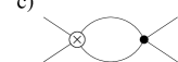
Figure 18: Graphs with an ultrasoft gluon, which contribute to the three-loop running of the Coulomb potential.

Because the energy in the potential loop is of order $mv^{2}$, the potential and the ultrasoft loops are not separable. The sum of the diagrams in the singlet channel reads

$$\mbox{Fig.\ \ref{figCoulombusoft}}\,=\,-\frac{4i}{3}\frac{C_{F}C_{A}^{3}}{8}\,\frac{[{\cal V}_{c}^{(T)}\mu_{S}^{2\epsilon}]^{3}\,[\alpha_{s}(m\nu^{2})\mu_{U}^{2\epsilon}]}{(4\pi)^{3}\,{\mathbf{k}}^{2}}\,\bigg{[}\,\frac{1}{\epsilon}+\ldots\,\bigg{]}$$ (79)

$$=-\frac{4i}{3}\frac{C_{F}C_{A}^{3}}{8}\,\frac{[\alpha_{s}(m\nu)]^{3}\,\alpha_{s}(m\nu^{2})\,\mu_{S}^{2\epsilon}}{{\mathbf{k}}^{2}}\,\bigg{[}\,\frac{1}{\epsilon}+\ln\Big{(}\frac{\mu_{U}^{2}}{E^{2}}\Big{)}+2\ln\Big{(}\frac{\mu_{S}^{2}}{\bf k^{2}}\Big{)}+\ldots\,\bigg{]}.\quad\quad$$

The total anomalous dimension in the singlet channel from the ultrasoft diagrams with respect to the velocity scaling parameter $\nu$ reads

$$\gamma_{U} = -\,\frac{4C_{F}C_{A}^{3}}{3}\,[\alpha_{s}(m\nu)]^{3}\,\alpha_{s}(m\nu^{2})\,.$$ (80)

After subtraction of subdivergences the three-loop soft graphs contain a UV divergence associated with the three-loop $\overline{\rm MS}$ $\beta$-function and a UV divergence that is induced by the UV divergence in the ultrasoft graphs discussed above. So the sum of all soft graphs gives the following contribution to the anomalous dimension

$$\gamma_{S} = C_{F}C_{A}^{3}\,[\alpha_{s}(m\nu)]^{4}+2C_{F}\beta_{2}\frac{[\alpha_{s}(m\nu)]^{4}}{(4\pi)^{2}}\,,$$ (81)

where $\beta_{2}=\frac{2857}{2}-\frac{5033}{18}\,n_{\ell}+\frac{325}{54}\,n_{\ell}^{2}\,.$ The result in Eq. (81) has been determined in Ref. [ $\!{}^{{\bf?}}$] without an explicit calculation. The first term on the RHS of Eq. (81) can be obtained directly from Eq. (79), because the overall dependence on the scales and on $\alpha_{s}$ of the corresponding divergence in the sum of the soft diagrams is proportional to $[\alpha_{s}(m\nu)\mu_{S}^{2\epsilon}]^{4}/\epsilon$. Taking into account the matching condition for the singlet coefficient at the hard scale, ${\cal V}_{c}^{(s)}(1)=-4\pi C_{F}\alpha_{s}(m)$, the full NNLL result reads $\!{}^{{\bf?}}$

$${\cal V}_{c}^{(s)}(\nu) = -4\pi C_{F}\alpha_{s}(m\nu)$$ (82)

$$+ \frac{8\pi C_{F}C_{A}^{3}}{3\beta_{0}}\alpha_{s}^{3}(m)\bigg{[}\frac{11}{4}-2z-\frac{z^{2}}{2}-\frac{z^{3}}{4}+4\ln(w)\bigg{]}\,,$$

where $z=\alpha_{s}(m\nu)/\alpha_{s}(m)$ and $w=\alpha_{s}(m\nu^{2})/\alpha_{s}(m)$. This result is needed for a NNLL order description of the non-relativistic $Q\bar{Q}$ dynamics. At the same order the coefficients of the $1/m^{2}$ potentials are needed at LL order, and the coefficients of the $1/(m|{\mathbf{k}}|)$ potentials are needed at NLL. The corresponding computations were carried out in Refs. [ $\!{}^{{\bf?}}$] and [ $\!{}^{{\bf?}}$], respectively.

To describe the production of $Q\bar{Q}$ pairs at NNLL order in $e^{+}e^{-}$ annihilation one needs the LL evolution of the coefficients $c_{2}$ and $c_{3}$ (see Eq. (73)) and the NNLL order evolution of $c_{1}$. The complete NNLL running of $c_{1}$ is not yet known. The NLL running was determined in Refs. [ $\!{}^{{\bf?},{\bf?}}$] and arises from UV divergent one- and two-loop graphs with insertions of the $1/(m|{\mathbf{k}}|)$ and $1/m^{2}$ potentials. At LL order $c_{1}(\nu)=1$, i.e. it does not run. The LL evolution of the axial-vector coefficient $c_{3}$ would be determined by UV divergent diagrams of order $\alpha_{s}v$, but such diagrams do not exist and $c_{3}(\nu)=c_{3}(1)=1$. The LL running of $c_{2}$ was determined in Ref. [ $\!{}^{{\bf?}}$] and arises from UV divergences in the ultrasoft graphs of order $\alpha_{s}v^{2}$ shown in Fig. 19.

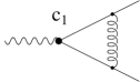
Figure 19: Graphs with an ultrasoft gluon with ${\mathbf{p}}.{\mathbf{A}}$ couplings which contribute to the running of $c_{2}(\nu)$.

The pull-up to the hard scale is provided by tadpole-like soft one-loop diagrams that vanish in dimensional regularization. The soft graphs arise from those in Fig. 19 by replacing the ultrasoft gluons by soft gluons and contracting the internal quark line to a point. The resulting anomalous dimension reads

$$\nu{\partial\over\partial\nu}c_{2}(\nu) = \frac{8C_{F}}{3\pi}\alpha_{s}(m\nu^{2})\,c_{1}(\nu)\,,$$ (83)

with the solution

$$c_{2}(\nu) = -\frac{1}{6}-\frac{8C_{F}}{3\beta_{0}}\ln\bigg{[}\frac{\alpha_{s}(m\nu^{2})}{\alpha_{s}(m)}\bigg{]}\,,$$ (84)

where Eq. (73) is used as the initial condition.

6 vNRQCD versus pNRQCD

The effective theories vNRQCD and pNRQCD are not equivalent. From the phenomenological point of view pNRQCD is the by fare more ambitious theory, because it was devised with the aim to treat systems with the hierarchy $m\gg mv\gg mv^{2}\gg\Lambda_{\rm QCD}$ as well as systems, where $\Lambda_{\rm QCD}$ is larger. In addition, it is supposed to treat, at the same time, systems with dynamical quark pairs and systems where the quarks are static.$\!{}^{{\bf?}}$ It is fair to say that some conceptual and technical aspects are not yet fully worked out, as the authors admit at some occasions, but it is argued that this does not affect the concepts of pNRQCD.$\!{}^{{\bf?}}$ On the other hand, vNRQCD has been designed only for the case $m\gg mv\gg mv^{2}\gg\Lambda_{\rm QCD}$, with the primary aim to provide a theory that is fully worked out technically and conceptually for this special case. The treatment of systems where $\Lambda_{\rm QCD}$ is larger is by construction difficult in vNRQCD. The theories pNRQCD and vNRQCD are not equivalent, because they lead to different predictions in the case $m\gg mv\gg mv^{2}\gg\Lambda_{\rm QCD}$.

It is very instructive to have a closer look at the mechanisms working in vNRQCD and pNRQCD by means of two examples. One, the order $m_{e}\alpha^{5}\ln\alpha$ Lamb shift in hydrogen in QED, where both effective theories agree, and the other, the Coulomb potential in the QCD Schrödinger equation for a color singlet $Q\bar{Q}$ pair, where both theories disagree. For simplicity, I will only concentrate on the mechanism of renormalization and the structure of logarithmic terms, which is sufficient to pinpoint the conceptual and technical differences. We note that both theories also disagree on their results for the $1/m$ potentials and the $Q\bar{Q}$ production currents. Those cases will not be discussed here, but the origin of the disagreement is the same as for the Schrödinger Coulomb potential.

6.1 Hydrogen Lamb Shift

The Lamb shift is the $2S_{1/2}$–$2P_{1/2}$ level splitting in the hydrogen spectrum. For infinite proton mass the order $m_{e}\alpha^{5}\ln\alpha$ term reads

$$\Delta E = -\frac{m_{e}\,\alpha^{5}}{3\,\pi}\,\ln\alpha\,,$$ (85)

where $\alpha=1/137$ is the fine structure constant and $m_{e}$ the electron mass. The result in Eq. (85) can be derived in vNRQED from the LL running of the ${\cal V}_{2}$ potential $\!{}^{{\bf?}}$ (Eq. (51)) and in the framework of pNRQED from the LL running of the $D_{d,s}^{(2)}$ potential (Eq. (33)) (see Ref. [ $\!{}^{{\bf?}}$] for a fixed order calculation).

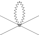
Figure 20: One-loop vNRQCD diagrams contributing to the LL anomalous dimension of ${\cal V}_{2}$.

In vNRQED the LL anomalous dimension of ${\cal V}_{2}$ comes from soft scattering loop diagrams, such as in Fig. 20a and b and from ultrasoft graphs, such as in Fig. 20c and d. In QED the leading soft two-fermion vertex is of order $1/m$ and there is no contribution from the soft diagram in Fig. 20a, if the proton mass is infinite. The soft diagram in Fig. 20b gives a massless tapole and vanishes in dimension regularization. Distinguishing between soft UV and IR divergences the result reads

Fig. 20b $$= -i\,\frac{2}{3m_{e}^{2}}\,[\alpha\,\mu_{S}^{2\epsilon}]^{2}\,\Big{[}\,\frac{1}{\epsilon_{\rm UV}}-\frac{1}{\epsilon_{\rm IR}}\,\Big{]}\,.$$ (86)

In Coulomb gauge the ultrasoft contributions are generated by ultrasoft photons with ${\mathbf{p}}.{\mathbf{A}}/m$ couplings dressing the Coulomb potential. Typical diagrams are displayed in Figs. 20c and d. For infinite proton mass only the diagram in Fig. 20c contributes. For on-shell external electrons ($E=\frac{\mathbf{p}^{2}}{2m}$) and including wave function renormalization constants the result reads

Fig. 20c $$= -i\,\frac{2}{3m_{e}^{2}}\,[\alpha\,\mu_{U}^{2\epsilon}]\,[\alpha\,\mu_{S}^{2\epsilon}]\,\Big{[}\,\frac{1}{\epsilon_{\rm UV}}-\frac{1}{\epsilon_{\rm IR}}\,\Big{]}\,.$$ (87)

The ultrasoft IR divergence in Eq. (87) is present also in full QED and not relevant for the renormalization procedure. This can be seen from the fact that the IR divergence is regularized for an off-shell electron with $E\neq\frac{\mathbf{p}^{2}}{2m}$. The ultrasoft UV divergence is canceled by a counter term in the unrenormalized ${\cal V}_{2}$ potential. The soft IR divergence is unphysical and does not exist in full QED. It is associated with the soft scale $m_{e}v$ and matches with the ultrasoft UV divergence, because in vNRQED the photon from full QED has been split into soft photon fields and an ultrasoft photon field. The full soft tadpole contribution pulls the ultrasoft running up to the hard scale. This feature exists for any ultrasoft running in vNRQCD. The final result for the LL anomalous dimension of ${\cal V}_{2}$ is determined from the ultrasoft UV divergence in Eq. (87) and reads 

$$\nu\frac{\partial}{\partial\nu}{\cal V}_{2}(\nu) = \frac{8}{3}\,\alpha^{2}\,.$$ (88)

In practical calculations the UV and IR divergences in soft loops do not need to be distinguished, because the pull-up is an automatic mechanism. This means that in the case of the Lamb shift the soft diagram would not have to be calculated at all. However, the IR divergences in ultrasoft loops have to be identified, because they are IR divergences of full QED and do not take part in the renormalization of vNRQED. The anomalous dimension in Eq. (88) can be trivially integrated giving

$${\cal V}_{2}(\nu) = -\frac{\pi\,\alpha}{2}+\frac{8}{3}\,\alpha^{2}\,\ln\nu\,,$$ (89)

where ${\cal V}_{2}(1)=-\frac{\pi\alpha}{2}$ is obtained from tree level matching. Interestingly, Eqs. (88) and (89) show that there is no infinite series of logarithmic terms $\propto\alpha(\alpha\ln\nu)^{n}$. The series terminates because $\alpha$ does not run and because there is no non-trivial mixing from other running operators.$\!{}^{{\bf?}}$ Since the ${\cal V}_{2}$ potential is the delta function in configuration space the contribution to the $2S_{1/2}$–$2P_{1/2}$ level splitting can be readily calculated,

$$\left\langle\,2S\,\left|-\frac{{\cal V}_{2}(\nu=\alpha)}{m_{e}^{2}}\,\right|\,2S\,\right\rangle = -\,\left|\Psi_{n=2}(0)\right|^{2}\,\frac{{\cal V}_{2}(\alpha)}{m_{e}^{2}}\,,$$ (90)

where $|\Psi_{n}(0)|^{2}=m_{e}^{3}\alpha^{3}/(\pi n^{3})$, which gives the known order $m_{e}\alpha^{5}\ln\alpha$ term in Eq. (85). A complete calculation of the order $m_{e}\alpha^{5}\ln\alpha$ Lamb shift for arbitrary masses in vNRQED can be found in Ref. [ $\!{}^{{\bf?}}$]. (The same work also contains the determination of the order $m_{e}\alpha^{8}\ln^{3}\alpha$ Lamb shift, the order $m_{e}\alpha^{7}\ln^{2}\alpha$ hyperfine splitting for arbitrary masses, and the order $\alpha^{2}\ln\alpha$ and $\alpha^{3}\ln^{2}\alpha$ corrections to ortho- and para-positronium decay in vNRQED using the renormalization group equations.)

In pNRQED the determination of $D_{d,s}^{(2)}$ is divided into two steps. In NRQED (supplemented by the $1/m$ expansion) the running of the Darwin coefficient $c_{D}$ is carried out from $\mu=m$ to $\mu=\mu_{s}$. The anomalous dimension of $c_{D}$ is obtained from one-loop vertex corrections and wave function diagrams such as displayed in Fig. 21

Figure 21: One-loop HQET vertex and wave function diagrams that contribute to the anomalous dimension of $c_{D}$. The photon in the loop couples with ${\mathbf{p}}.{\mathbf{A}}/m_{e}$ and the external photon with $A^{0}$.

and has been carried out before in the framework of HQET.$\!{}^{{\bf?}}$ In these diagrams the photon in the loop couples with ${\mathbf{p}}.{\mathbf{A}}/m_{e}$ to the electron. For on-shell electrons with momenta $\mathbf{p}$ and $\mathbf{p}^{\prime}$ the sum of diagrams relevant for the renormalization of $c_{D}$ reads

Figs. 21 $$= -\frac{i}{6\pi}\,\frac{(\mathbf{p}-\mathbf{p}^{\prime})^{2}}{m_{e}^{2}}\,[g\,\mu^{\epsilon}]\,[\alpha\,\mu^{2\epsilon}]\,\Big{[}\,\frac{1}{\epsilon_{\rm UV}}-\frac{1}{\epsilon_{\rm IR}}\,\Big{]}\,,$$ (91)

when IR and UV divergences are distinguished. Interestingly, the result seems to be equivalent to the soft vNRQCD amplitude in Eq. (87), when the photon exchange to the proton is included. However, here the IR divergence is the IR divergence from full QED, because NRQED is supposed to describe the whole momentum space below the scale $m_{e}$. At this point this observation seems to be only a curious fact, but it is at the heart of the conceptual differences between vNRQCD and pNRQCD. The UV divergence in Eq. (91) is canceled by a counter term in the unrenormalized $c_{D}$ interaction and the anomalous dimension of $c_{D}$ reads

$$\mu\frac{\partial}{\partial\mu}c_{D}(\mu) = -\frac{8\,\alpha}{3\,\pi}$$ (92)

with the solution

$$c_{D}(\mu) = 1-\frac{8\,\alpha}{3\,\pi}\,\ln\Big{(}\frac{\mu}{m_{e}}\Big{)}\,,$$ (93)

where $c_{D}(m_{e})=1$ is obtained from tree level matching. The second step is carried out in pNRQED. The matching condition for the $D_{d,s}^{(2)}$ potential at $\mu=\mu_{s}$ is obtained by calculating the NRQED Born scattering diagram in Fig. 22

Figure 22: NRQCD diagram contributing to the Born matching condition of the $D_{d,s}^{(2)}$ potential in pNRQCD.

for off-shell electron momenta $(0,\mathbf{p})$ and $(0,\mathbf{p}^{\prime})$ for the incoming and outgoing electron, respectively. The little square indicates the $c_{D}$-coupling. This gives

$$D_{d,s}^{(2)}(\mu=\mu_{s}) = \frac{\alpha}{2}\,c_{D}(\mu_{s})\,=\,\frac{\alpha}{2}-\frac{4\,\alpha^{2}}{3\,\pi}\ln\Big{(}\frac{\mu_{s}}{m_{e}}\Big{)}\,.$$ (94)

The running of $D_{d,s}^{(2)}$ in pNRQCD is determined as described in Sec. 4 from the ultrasoft one-loop diagrams in Fig. 6b in the $1/m$ expansion. For electrons with external momenta $(0,\mathbf{p})$ and $(0,\mathbf{p}^{\prime})$ the result reads

Fig. 6b $$= -i\,\frac{2\,\alpha}{3m_{e}^{2}}\,[\alpha\,\mu^{2\epsilon}]\,\Big{[}\,\frac{1}{\epsilon_{\rm UV}}-\frac{1}{\epsilon_{\rm IR}}\,\Big{]}\,.$$ (95)

The IR divergence is again the full QED IR divergence. The UV divergence is canceled by a counterterm in the unrenormalized $D_{d,s}^{(2)}$ potential and leads to the following LL anomalous dimension for $D_{d,s}^{(2)}$,

$$\frac{d}{d\ln\mu}D_{d,s}^{(2)}(\mu) = -\frac{4\,\alpha^{2}}{3\,\pi}\,.$$ (96)

This is again integrated trivially giving

$$D_{d,s}^{(2)}(\mu_{u}) = D_{d,s}^{(2)}(\mu_{s})-\frac{4\,\alpha^{2}}{3\,\pi}\,\ln\Big{(}\frac{\mu_{u}}{\mu_{s}}\Big{)}\,=\,\frac{\alpha}{2}-\frac{4\,\alpha^{2}}{3\,\pi}\ln\Big{(}\frac{\mu_{u}}{m_{e}}\Big{)}$$ (97)

$$= \frac{\alpha}{2}\,c_{D}(\mu_{u})$$

at the scale $\mu=\mu_{u}$. For $\mu_{u}=m_{e}\alpha^{2}$ this agrees with ${\cal V}_{2}$ up to a convention-dependent factor and also leads to Eq. (85) for the order $m_{e}\alpha^{5}\ln\alpha$ Lamb shift. Comparing the computations we see that the difference between vNRQED and pNRQED appears to be simply that the running is distributed in a different way. In vNRQED running happens in one step and in pNRQED it happens in two steps. Agreement is in fact found for the LL running of all $1/m^{2}$ potentials in vNRQCD (Refs. [ $\!{}^{{\bf?},{\bf?}}$]) and pNRQCD (Ref. [ $\!{}^{{\bf?}}$]).

One of the main differences between QED and QCD is that the coupling constant runs itself. If we consider the Lamb shift of muonic hydrogen and treat the electron as massless we can “simulate”, in a simplified way, one difference of the calculation presented above to the QCD case. If massless electrons are included, the fine structure constant becomes scale-dependent using let’s say the $\overline{\rm MS}$ renormalization scheme. This makes the couplings in all potentials scale-dependent and makes the $2S_{1/2}$–$2P_{1/2}$ level splitting more complicated. As shown in Sec. 6.2, the $\alpha$ in the Coulomb-potential has to be set at the scale $\mu_{s}$ or $m\nu$ and, as the consequence, also the $\alpha$ in the wavefunction at the origin in Eq. (90). In addition, also the $\alpha$ in the Spin-Orbit potential (the $D^{(2)}_{LS,s}$ term in Eq. (33) and the ${\cal V}_{\Lambda}$ terms in Eq. (50)), has to be set at the scale $\mu_{s}$ or $m\nu$ and now contributes logarithmic terms to the $2S_{1/2}$–$2P_{1/2}$ level splitting. For the purpose of this discussion we only consider the coefficients $D_{d,s}^{(2)}$ and ${\cal V}_{2}$ in some detail, because they contain a non-trivial ultrasoft running involving the scales $\mu_{u}$ or $m\nu^{2}$. In the pNRQCD computation for $c_{D}$ the coupling in the anomalous dimension in Eq. (92) is $\alpha(\mu)$ and the result for $c_{D}$ is

$$c_{D}(\mu) = 1+\frac{16}{3\,\bar{\beta}_{0}}\,\ln\bigg{(}\frac{\alpha(\mu)}{\alpha(m_{\mu})}\bigg{)}\,,$$ (98)

where $\bar{\beta}_{0}=-\frac{4}{3}n_{\ell}$, $n_{\ell}=1$. The $\alpha$ in the matching condition of Eq. (94) is evaluated at $\mu=\mu_{s}$ and the LL anomalous dimension for $D_{d,s}^{(2)}$ reads

$$\frac{d}{d\ln\mu}D_{d,s}^{(2)}(\mu) = -\frac{4\,\alpha(\mu_{s})}{3\,\pi}\,\alpha(\mu)\,.$$ (99)

The coefficient of the LL static potential is set at the scale $\mu_{s}$ and does not run below $\mu_{s}$. The solution just reads

$$D_{d,s}^{(2)}(\mu_{u})=\frac{\alpha(\mu_{s})}{2}c_{D}(\mu_{u})\,.$$

In vNRQED with massless electrons the anomalous dimension for ${\cal V}_{2}$ also gets a contribution from loops in Fig. 20a and b where the soft photons are replaced by soft (massless) electrons. The modified version of Eq. (88) then reads

$$\frac{d}{d\ln\nu}{\cal V}_{2}(\nu) = \frac{8}{3}\,\alpha(m_{\mu}\nu)\,\alpha(m_{\mu}\nu^{2})+\frac{\bar{\beta}_{0}}{4}\,[\alpha(m_{\mu}\nu)]^{2}\,c_{4\mu 2e}(\nu)\,,$$

$$c_{4\mu 2e}(\nu) = c_{D}(m_{\mu}\nu^{2})\,,$$ (100)

where $c_{4\mu 2e}$ is the coefficient of the 6-fermion operator contained in Fig. 20b. (This type of operators, involving four heavy quarks and two soft gluons or massless quarks, has been missed in Ref. [ $\!{}^{{\bf?}}$]. Their numerical contribution is small $\!{}^{{\bf?}}$ and does not affect conclusions drawn based on the results of Ref. [ $\!{}^{{\bf?}}$].)

It turns out that this coefficient is equal to the $c_{D}$ obtained in NRQED at the scale $\mu=m_{\mu}\nu^{2}$. Integrating Eq. (100) with the initial condition ${\cal V}_{2}(1)=-\pi\alpha(m)/2$ gives

$${\cal V}_{2}(\nu) = -\frac{\pi\,\alpha(m_{\mu}\nu)}{2}\,c_{D}(m_{\mu}\nu^{2})\,,$$ (101)

which agrees again with the pNRQED result up to a convention-dependent factor. The vNRQCD and pNRQCD computations agree, because only one-loop diagrams contribute to the LL anomalous dimensions of the $1/m^{2}$ potentials. So at this level it seems to be merely a choice of convention whether one uses vNRQCD or pNRQCD, because the running is just distributed in a different way. The actual reason for agreement, however, it that at LL order the (one-loop) diagrams cannot contain non-separable ultrasoft and potential loops at the same time, which connects in a subtle way the evolution with respect to soft and ultrasoft scales.

6.2 Schrödinger Coulomb Potential at NNLL Order

The subtle difference in the renormalization of vNRQCD and pNRQCD becomes apparent beyond the LL approximation, when non-trivial multi-loop diagrams with UV divergences contain loops dominated by the ultrasoft and the potential region. Examples are the Coulomb potential $\propto 1/{\mathbf{k}}^{2}$ in the NNLL order Schrödinger equation for a color singlet $Q\bar{Q}$ pair (see Ref. [ $\!{}^{{\bf?}}$] for vNRQCD and Ref. [ $\!{}^{{\bf?}}$] for pNRQCD) or the $1/(m|{\mathbf{k}}|)$ potential at NLL order (see Ref. [ $\!{}^{{\bf?}}$] for vNRQCD and Refs. [ $\!{}^{{\bf?},{\bf?}}$] for pNRQCD). Because the $1/(m|{\mathbf{k}}|)$ potentials contribute to the NLL running of the $Q\bar{Q}$ production current, vNRQCD and pNRQCD predictions also differ for the latter case (see Refs. [ $\!{}^{{\bf?},{\bf?}}$] for vNRQCD and Ref. [ $\!{}^{{\bf?}}$] for pNRQCD). Let us discuss the NNLL order Coulomb potential that appears in the Schrödinger equation. Its determination in vNRQCD and pNRQCD has already been described in previous sections and will not be repeated in detail.

In vNRQCD the NNLL $1/(\mathbf{p}-\mathbf{p}^{\prime})^{2}$ potential that appears in the Schrödinger equation, called $V_{c}^{v}$ in the following, consists of the sum of the Coulomb potential ${\cal V}_{c}{(s)}/(\mathbf{p}-\mathbf{p}^{\prime})^{2}$ at NNLL order and the time-ordered products of soft vertices proportional to $1/(\mathbf{p}-\mathbf{p}^{\prime})^{2}$ at one (Figs. 12c and Eq. (77)) and two loops (see Figs. 17) that determine the running of ${\cal V}_{c}$ at LL and NLL order. Im momentum space for $D=4$ the sum is ($\mathbf{k}=(\mathbf{p}-\mathbf{p}^{\prime})$)

$$\tilde{V}_{c}^{v}({\mathbf{p}},{\mathbf{q}})=\frac{{\cal{V}}_{c}^{(s)}(\nu)}{{\mathbf{k}}^{2}}\,-\,\frac{4\pi C_{F}\,\alpha_{s}(m\nu)}{\mathbf{k}^{2}}\bigg{\{}\frac{\alpha_{s}(m\nu)}{4\pi}\,\bigg{[}-\beta_{0}\,\ln\Big{(}\frac{\mathbf{k}^{2}}{m^{2}\nu^{2}}\Big{)}+a_{1}\bigg{]}$$ (102)

$$+\bigg{(}\frac{\alpha_{s}(\mu_{s})}{4\pi}\bigg{)}^{2}\bigg{[}\beta_{0}^{2}\,\ln^{2}\Big{(}\frac{\mathbf{k}^{2}}{m^{2}\nu^{2}}\Big{)}-\Big{(}2\,\beta_{0}\,a_{1}+\beta_{1}\Big{)}\,\ln\Big{(}\frac{\mathbf{k}^{2}}{m^{2}\nu^{2}}\Big{)}+a_{2}\bigg{]}\,\bigg{\}}\qquad$$

$$= \Big{[}\mbox{Eq.\ (\ref{staticpotentialschroeder})}\Big{]}+\frac{8\pi C_{F}C_{A}^{3}}{3\beta_{0}\,{\mathbf{k}}^{2}}\,\alpha_{s}^{3}(m)\,\bigg{[}\frac{11}{4}-2z-\frac{z^{2}}{2}-\frac{z^{3}}{4}+4\ln(w)\bigg{]}\,,$$

where $z=\alpha_{s}(m\nu)/\alpha_{s}(m)$ and $w=\alpha_{s}(m\nu^{2})/\alpha_{s}(m\nu)$. In principle it is inappropriate to consider the soft time-ordered products together with the ${\cal V}_{c}^{(s)}$ term as a single quantity for $D=4$ because they are matrix elements depending non-trivially on $D=4-2\epsilon$ dimensions. Therefore, they should not be considered for $\epsilon\to 0$ independently of the other matrix elements relevant for a given process. However, as long as insertions of the soft time-ordered products do not generate UV divergences relevant for the process, Eq. (102) can be used. This is also the case for the NNLL order description of $Q\bar{Q}$ pairs, when the quarks are stable.

In the pNRQCD framework the NNLL $1/(\mathbf{p}-\mathbf{p}^{\prime})^{2}$ potential that appears in the Schrödinger equation, called $V_{c}^{p}$ in the following, is obtained directly from the two-step matching and running through NRQCD and pNRQCD. The NNLL result reads

$$\tilde{V}_{c}^{p}(\mathbf{p},\mathbf{q}) = -\frac{4\pi C_{F}\alpha_{V_{s}}(\mu_{u},\mu_{s})}{\mathbf{k}^{2}}$$ (103)

$$= \Big{[}\mbox{Eq.\ (\ref{staticpotentialschroeder})}\Big{]}-\frac{2\pi C_{F}C_{A}^{3}}{3\beta_{0}\,{\mathbf{k}}^{2}}\alpha_{s}^{3}(\mu_{s})\ln\bigg{(}\frac{\alpha_{s}(\mu_{s})}{\alpha_{s}(\mu_{u})}\bigg{)}\,.$$

The first term is the two-loop pNRQCD matching condition and the second term arises from the pNRQCD running from $\mu_{s}$ to $\mu_{u}$. All computations are carried out in the static limit abandoning the non-relativistic power counting for $Q\bar{Q}$ pairs because otherwise the NRQCD computations cannot be properly defined. It is one of the most important assumptions in the pNRQCD framework that the static calculation of the running coefficients can be applied also for moving dynamical quark pairs.

Comparing Eqs. (102) and (103) one finds disagreement in the contributions associated with the ultrasoft gluons. Expanding the second term in Eq. (102) (times a factor ${\mathbf{k}}^{2}$) in $\alpha_{s}(m)$, we find

$$-\frac{1}{3}\,{C_{F}C_{A}^{3}}\,\alpha_{s}^{4}(m)\ln(\nu)+\frac{2\beta_{0}}{3\pi}\,{C_{F}C_{A}^{3}}\,\alpha_{s}^{5}(m)\ln^{2}(\nu)+\ldots\,.$$ (104)

The analogous result for the static calculation in Eq. (103) for $\mu_{s}=m\nu$ and $\mu_{u}=m\nu^{2}$ reads

$$-\frac{1}{3}\,{C_{F}C_{A}^{3}}\,\alpha_{s}^{4}(m)\ln(\nu)+\frac{3\beta_{0}}{4\pi}\,{C_{F}C_{A}^{3}}\,\alpha_{s}^{5}(m)\ln^{2}(\nu)+\ldots\,.$$ (105)

The single $\ln\nu$ terms agree, but the higher order logarithms differ. From the phenomenological point of view the difference is quite small for most applications, but both theories claim to sum the correct higher order logarithms.

In vNRQCD the result arises from the UV divergences in the three-loop ultrasoft-potential diagrams in Fig. 18 and the associated UV divergences in three-loop soft diagrams. The individual quark propagators $i/(k_{0}-{\mathbf{k}}^{2}/m+i\delta)$ in the ultrasoft-potential diagrams describe dynamical quarks. The resulting anomalous dimension in Eq. (80) describes running from $\nu=1$ to $\nu=v$ and includes the scale-dependence from all three loops, i.e. the factors $\mu_{S}^{4\epsilon}\,\mu_{U}^{2\epsilon}$ for the ultrasoft-potential diagrams and $\mu_{S}^{6\epsilon}$ for the soft as well as the scale-dependence of all the coupling constants that occur in the diagrams. In pNRQCD the result arises from the UV divergence of the one-loop diagram Fig. 5 with one ultrasoft gluon and a static $Q\bar{Q}$ propagator $i/(i\partial_{0}+(\frac{1}{2}C_{A}-C_{F})\alpha_{V_{o}}/r)$. This propagator sums an infinite number of static potential rungs in $D=4$ dimensions. The resulting anomalous dimension in Eq. (40) describes running from $\mu=\mu_{s}\sim mv$ to $\mu=\mu_{u}\sim mv^{2}$ and includes only the scale dependence of the ultrasoft loop, i.e. the factor $\mu^{2\epsilon}$ and the ultrasoft coupling $\alpha_{s}(\mu)$. The quarks in the loops with the Coulomb rungs are not dynamical. Clearly, if the calculation would involve only true one-loop diagrams, as was the case for the Lamb shift discussed before, we would find again agreement, because loops involving multiple iterations of potentials wouldn’t exist.

At the conceptual level the difference can be understood as the difference between a calculation for static and dynamical quarks. In the dynamical vNRQCD calculation the correlation between soft and ultrasoft scales through the quark equation of motion is maintained at all times. In the static pNRQCD calculation the scale correlation is broken at intermediate steps through the $1/m$ expansion, i.e. energy and three-momentum are treated independently. The discussion above shows that dynamical and static $Q\bar{Q}$ systems are different. In particular, it can be problematic to use results obtained in static quark systems for problems involving dynamical quarks.

At this point it is, once more, instructive to see with a very simple example $\!{}^{{\bf?}}$ how the $1/m$ expansion breaks the non-relativistic power counting. In the static calculation the time-ordered product of a $1/(m|\mathbf{k}|)$ and a $1/\mathbf{k}^{2}$ potential is

$$\int\frac{d^{4}k}{(2\pi)^{4}}\,\frac{1}{m|\mathbf{k}|}\,\frac{1}{\left(k_{0}+i\delta\right)}\,\frac{1}{\left(k_{0}-i\delta\right)}\,\frac{1}{\mathbf{k}^{2}} \,\sim\, \frac{1}{m}$$ (106)

and hence suppressed by $1/m$.

Figure 23: Loop graph with an insertion of the $1/(m|{\bf k})$ and $1/{\bf k^{2}}$ potentials.

In the dynamical calculation (see Fig. 23) the time-ordered product of a $1/(m|\mathbf{k}|)$ and a $1/\mathbf{k}^{2}$ potential is

$$\int\frac{d^{4}k}{(2\pi)^{4}}\,\frac{1}{m|\mathbf{k}|}\,\frac{1}{\left(k_{0}-\frac{\mathbf{k}^{2}}{2m}+i\delta\right)}\,\frac{1}{\left(k_{0}+\frac{\mathbf{k}^{2}}{2m}-i\delta\right)}\,\frac{1}{\mathbf{k}^{2}}$$ (107)

$$\sim \int\frac{d^{3}k}{(2\pi)^{3}}\,\frac{1}{m|\mathbf{k}|}\,\frac{m}{\left(\mathbf{k}^{2}-i\delta\right)}\,\frac{1}{\mathbf{k}^{2}}\,\sim\,1$$

and of order $1$.

7 Heavy Quark Mass and Renormalons

In the discussions of the previous sections on non-relativistic effective theories we have assumed the pole mass definition $m$ for the heavy quarks. From the effective Lagrangians one can derive the one-particle-irreducible two-point function for a quark with energy $E=\sqrt{s}-2m_{\rm pole}$, $\sqrt{s}$ being the total center-of-mass energy, and three-momentum ${\mathbf{p}}$,

$$E\,-\,\frac{{\mathbf{p}}^{2}}{2m_{\rm pole}}\,+\,\frac{{\mathbf{p}}^{4}}{8m^{3}_{\rm pole}}\,+\,\ldots\,,$$ (108)

which vanishes for an on-shell quark in the center-of-mass frame ($E={\mathbf{p}}=0$). The on-shell condition is useful for the determination of matching conditions and anomalous dimensions in the effective theories. So at this stage the use of the pole mass definition is appropriate and useful. For a general mass definition $M=m_{\rm pole}+\delta M$ the effective Lagrangians contain additional bilinear quark operators $\delta M\psi^{\dagger}\psi$, $\delta M\psi^{\dagger}\frac{{\mathbf{p}}^{2}}{M^{2}}\psi$, etc., and the one-particle-irreducible two-point function for a quark reads

$$E_{M}\,+\,2\delta M\,-\,\frac{{\mathbf{p}}^{2}}{2M}\bigg{(}1+\frac{\delta M}{M}+\ldots\bigg{)}\,+\,\frac{{\mathbf{p}}^{4}}{8M^{3}}\,+\,\ldots\,,$$ (109)

where $E_{M}=\sqrt{s}-2M$.

7.1 Pole Mass and Static Potential

Since quark masses, just like coupling constants such as $\alpha_{s}$, are parameters of the Lagrangian and not physical observables, in principle any quark mass definition can be employed as long as its perturbative definition is known and well defined. A suitable mass definition should also have reasonable properties such as being gauge-invariant and IR-safe. The pole mass definition certainly belongs to this class.$\!{}^{{\bf?}}$ However, there are good reasons not to use the pole mass definition for the analysis of experimental data, because it induces artificially large perturbative corrections. In the framework of the theory of asymptotic series these perturbative corrections can, with certain assumptions on their large order behavior, be interpreted as an intrinsic ambiguity of the pole mass definition of the order $\Lambda_{\rm QCD}\approx 300$ MeV caused by a strong linear sensitivity to small momenta of order $\Lambda_{\rm QCD}$. (The exact amount of the uncertainty is difficult to estimate, and I have just given a personal (and probably biased) number to be definite. It is also not intended to rely on a specific scheme when the notion of “$\Lambda_{\rm QCD}$” is used.) This unpleasant property is, at least from the perturbative point of view, not characteristic for all quark mass definitions. For the pole mass this property was first discussed in the analysis of B meson decays in the framework of HQET.$\!{}^{{\bf?},{\bf?}}$ In the context of non-relativistic $Q\bar{Q}$ systems the same problem was first realized by Aglietti and Ligeti $\!{}^{{\bf?}}$ in an analysis of the large order behavior of the perturbative static $Q\bar{Q}$ potential. Initially, however, the connection to the properties of the pole mass parameters was not noticed. The problems associated with the pole mass definition are not academic. For heavy quarkonium systems it is important to consider the issue seriously, since the parametric perturbative uncertainty of present next-to-next-to-leading order computations is already at a level where an ambiguity of a mass definition of order $\Lambda_{\rm QCD}$ is relevant.

Aglietti and Ligeti $\!{}^{{\bf?}}$ considered the color singlet static potential in the “large-$\beta_{0}$” approximation,

$$\tilde{V}_{\rm static}^{\beta_{0}}({\mathbf{k}}) = -\frac{4\pi C_{F}\alpha_{s}(\mu)}{{\mathbf{k}}^{2}}\,\sum\limits_{n=0}^{\infty}\bigg{[}-\frac{\alpha_{s}(\mu)}{4\pi}\,\beta_{0}\,\ln\Big{(}\frac{{\mathbf{k}}^{2}e^{c}}{\mu^{2}}\Big{)}\,\bigg{]}^{n}\,,$$ (110)

where $c=-5/3$ in the $\overline{\rm MS}$ scheme. The large-$\beta_{0}$ approximation assumes that the highest power of $\beta_{0}$ in each order of perturbation theory dominates numerically the rest of the contributions.$\!{}^{{\bf?}}$ At this point the distinction between the static pNRQCD potential and the Schrödinger Coulomb potential in vNRQCD is irrelevant, because the large-$\beta_{0}$ approximation is the same in both cases. The large order behavior can then be analyzed through the Borel transform of $\tilde{V}_{\rm static}^{\beta_{0}}$ with respect to $\alpha_{s}\beta_{0}/(4\pi)$,

$$B[\tilde{V}_{\rm static}^{\beta_{0}}](u) = -\frac{16\pi^{2}C_{F}}{\beta_{0}\,{\mathbf{k}}^{2}}\,\sum\limits_{n=0}^{\infty}\frac{1}{n!}\,\bigg{[}-u\,\beta_{0}\,\ln\Big{(}\frac{{\mathbf{k}}^{2}e^{c}}{\mu^{2}}\Big{)}\,\bigg{]}^{n}$$ (111)

$$= -\frac{16\pi^{2}C_{F}}{\beta_{0}\,{\mathbf{k}}^{2}}\,\frac{\mu^{2u}e^{-cu}}{({\mathbf{k}}^{2})^{1+u}}\,.$$

The inverse Borel transform reads

$$\tilde{V}_{\rm stat}^{\beta_{0}}({\mathbf{k}})=\int_{0}^{\infty}du\,B[\tilde{V}_{\rm stat}^{\beta_{0}}](u)\,\exp\Big{(}-\frac{4\pi u}{\beta_{0}\alpha_{s}(\mu)}\Big{)}\,.$$

The impact of the large order behavior of Eq. (110) in bound state calculations can be visualized by considering the static potential in configuration space, describing the static energy of a $Q\bar{Q}$ pair with distance $r\ll\frac{1}{\Lambda_{\rm QCD}}$ in the pole mass scheme,

$$B[V_{\rm static}^{\beta_{0}}](u) = \int\frac{d^{3}{\mathbf{k}}}{(2\pi)^{3}}\,e^{i{\mathbf{k}}.{\mathbf{r}}}\,B[\tilde{V}_{\rm static}^{\beta_{0}}](u)$$ (112)

$$= -\frac{4C_{F}e^{-cu}}{\beta_{0}\,r}\,(\mu r)^{2u}\,\frac{\Gamma(\mbox{$\frac{1}{2}+u$})\Gamma(\mbox{$\frac{1}{2}-u$})}{\Gamma(2u+1)}\,.$$

The RHS of Eq. (112) has poles on the positive real axis at $u=(2k+1)/2$, $k=0,1,2,3,\ldots$, with residues $\propto(\mu r)^{2k+1}/r$. These poles cause ambiguities in $V_{\rm stat}^{\beta_{0}}(r)$ proportional to

$$\frac{(\mu r)^{2k+1}}{r}\exp\Big{(}-\frac{4\pi}{\beta_{0}\alpha_{s}(\mu)}\frac{2k+1}{2}\Big{)}\sim\frac{(\Lambda_{\rm QCD}\,r)^{2k+1}}{r}\,,$$

since there is no a priori prescription how the poles on the positive real axis should be treated in the inverse Borel transformation. The pole closest to the origin at $u=1/2$ is dominant and causes an ambiguity of order $\Lambda_{\rm QCD}$. It corresponds to an asymptotic large order behavior of $V_{\rm stat}^{\beta_{0}}(r)$ proportional to

$$\alpha_{s}(\mu)\,\mu\,\left(\frac{\alpha_{s}(\mu)\beta_{0}}{2\pi}\right)^{n}n!\,\,.$$

One might wonder how such an $r$-independent behavior can arise in the static potential, which has an overall factor $1/r$. It was shown in Ref. [ $\!{}^{{\bf?}}$] that it arises from an exponential structure of the $\ln(\mu r)$ terms in the order $\alpha_{s}^{n+1}$ term in $V_{\rm stat}^{\beta_{0}}(r)$ of the form

$$\sim\frac{\alpha_{s}}{r}\left(\frac{\alpha_{s}\beta_{0}}{2\pi}\right)^{n}\,n!\,\bigg{[}\,\frac{1}{(n-1)!}\ln^{n-1}(\mu r)+\ldots+\frac{1}{2}\ln^{2}(\mu r)+\ln(\mu r)+1\,\bigg{]}$$ (113)

$$\approx \frac{\alpha_{s}}{r}\left(\frac{\alpha_{s}\beta_{0}}{2\pi}\right)^{n}\,n!\,\,e^{\ln(\mu r)}\,=\,\alpha_{s}\,\mu\,\left(\frac{\alpha_{s}\beta_{0}}{2\pi}\right)^{n}\,n!\,.\hskip 113.81102pt$$

It should be noted that the large-$\beta_{0}$ approximation is just a heuristic concept. However, explicit multi-loop calculations for example for the perturbative relation between $\overline{\rm MS}$ and pole mass $\!{}^{{\bf?},{\bf?},{\bf?}}$ have shown a remarkable consistency with the large-$\beta_{0}$ approximation. On the other hand, it has also been reported $\!{}^{{\bf?},{\bf?}}$ that the large-$\beta_{0}$ approximation gives only order of magnitude estimates for higher order corrections in mass relations that do not involve the pole mass definition. Numerical evidence for the bad behavior of the static potential in configuration space was in fact noticed quite early, see e.g. Refs. [ $\!{}^{{\bf?}}$], but the observations were not interpreted as a consequence of the pole mass definition.

If the previously described large order behavior would be real, the determination of perturbative quark mass parameters would be forever limited to an uncertainty of order $\Lambda_{\rm QCD}$. However, it was found by Hoang et al. $\!{}^{{\bf?}}$ and Beneke $\!{}^{{\bf?}}$ (see also Refs. [ $\!{}^{{\bf?}}$]) that the ambiguity of order $\Lambda_{\rm QCD}$ is unphysical and merely an artifact of using the pole mass definition. The pole mass counterterm subtracts, apart from the usual UV divergent term, also a finite piece that correspond to the static quark selfenergy,

$$\frac{1}{2}\int\frac{d^{3}{\mathbf{k}}^{3}}{(2\pi)^{3}}\tilde{V}_{\rm stat}({\mathbf{k}})\,.$$ (114)

This expression is just the leading term in the non-relativistic expansion of the finite piece in the pole mass counterterm. Its asymptotic large order behavior is exactly $1/2$ times the asymptotic large order behavior of the static potential displayed in Eq. (113). If a mass definition is chosen that does not subtract the static selfenergy, the order $\Lambda_{\rm QCD}$ ambiguity and the corresponding bad large order behavior of the perturbative series described above do not arise in the first place. Hoang et al. $\!{}^{{\bf?}}$ and Beneke $\!{}^{{\bf?}}$ demonstrated that the total static energy,

$$E_{\rm stat} = 2m_{\rm pole}\,+\,V_{\rm stat}(r)\,,$$ (115)

is free of the ambiguity of order $\Lambda_{\rm QCD}$, at least from the point of view of perturbation theory.

It was shown by Smith and Willenbrock $\!{}^{{\bf?}}$ that even if the quark is unstable and decays with a finite lifetime smaller than $1/\Lambda_{\rm QCD}$, the static quark selfenergy in Eq. (114) produces the same large corrections described above. Thus the problematic behavior of the pole mass definition remains also for short-lived quarks such as the top quark with $\Gamma_{t}\approx 1.5$ GeV in the Standard Model.

The previous discussion disqualifies the pole mass a priori for the use in analyses of experimental data, since it induces artificially large corrections that are compensated e.g. by shifts in the pole mass value itself, when higher order corrections are included. In principle, the pole mass can still be employed as an order- and scale-dependent correlated quantity, similar to the value of a matrix element. $\!{}^{{\bf?}}$ In such an approach the large perturbative corrections associated with the pole mass are contained in its numerical value. Since these corrections depend on the order and on the choice for renormalization scales and couplings, the numerical value of the pole mass needs to be treated as a function of these parameters in order to achieve the proper cancellation of the large corrections, if the pole mass value is used in computations for other mass-dependent quantities. It should be noted, however, that this strategy can become increasingly unreliable for orders $n$ where the corrections induced by the pole mass are large enough that their numerical cancellation is incomplete. Results for analyses in the pole mass scheme for the $t\bar{t}$ production close to threshold in $e^{+}e^{-}$ annihilation and for bottom mass extraction from $b\bar{b}$ sum rules are discussed in Secs. 9 and 10.

The subdominant ambiguity in the static potential is order $\Lambda_{\rm QCD}^{2}r\sim\Lambda_{\rm QCD}^{2}/(m\alpha_{s})$ and quite small parametrically. The associated large order behavior of the perturbative series was analyzed by Brambilla et al. in Ref. [ $\!{}^{{\bf?}}$], and it was found that it cancels with the large order behavior of the leading ultrasoft corrections shown in Fig. 5 coming from two insertions of the ${\mathbf{r}}.{\mathbf{E}}$ interaction. The cancellation is independent of the choice for the quark mass definition. The ambiguity of order $\Lambda_{\rm QCD}^{2}r$ can be ignored for any practical analysis of the non-relativistic $Q\bar{Q}$ dynamics.

7.2 $\overline{\rm MS}$ Mass and Threshold Masses

To avoid the problems of the pole mass definition it is advantageous to use quark mass definitions that are less sensitive to low momenta and do not contain the static quark selfenergy in the mass counter term. Such quark mass definitions are called “short-distance” masses and have a parametric ambiguity or order $\Lambda_{\rm QCD}^{2}/M$ or smaller. In principle, the most natural choice of a short-distance mass would be the $\overline{\rm MS}$ (or MS) mass, because its mass counter term subtracts only the UV poles $\propto 1/\epsilon^{n}$ and does not contain any infrared-sensitive subtraction. This means that the $\overline{\rm MS}$ mass is only sensitive to scales of order or larger than $m$ and that it is from the conceptual point of view not allowed to lower the scale of the $\overline{\rm MS}$ mass below $m$. The relation between the pole mass and the $\overline{\rm MS}$ mass $\overline{m}(\overline{m})$ reads ($\bar{\alpha}_{s}=\alpha_{s}^{(n_{\ell}+1)}(\overline{m}(\overline{m}))$)

$$r_{m} \equiv \frac{m_{\rm pole}}{\overline{m}(\overline{m})}\,=\,1+\frac{4\bar{\alpha}_{s}}{3\pi}+\Big{(}\frac{\bar{\alpha}_{s}}{\pi}\Big{)}^{2}\,\Big{(}13.4434-1.0414n_{\ell}\Big{)}$$ (116)

$$\qquad\quad+\Big{(}\frac{\bar{\alpha}_{s}}{\pi}\Big{)}^{3}\,\Big{(}190.595-26.655n_{\ell}+0.6527n_{\ell}^{2}\Big{)}+\ldots$$

for $n_{\ell}$ massless light quark species. The two-loop correction was determined in Ref. [ $\!{}^{{\bf?}}$] and the three-loop term in Ref. [ $\!{}^{{\bf?}}$] (see Ref. [ $\!{}^{{\bf?}}$] for a numerical computation). For b quarks with $\bar{\alpha}_{s}=0.22$ and $n_{\ell}=4$ the series on the RHS of Eq. (116) reads $1-0.093+0.045+0.032$. Its rather poor convergence properties at already low orders illustrate the infrared sensitivity of the pole mass. The use of the $\overline{\rm MS}$ mass for non-relativistic $Q\bar{Q}$ systems would in principle be welcome, because it is also the preferred mass definition for high energy processes or electroweak precision observables. Unfortunately, the $\overline{\rm MS}$ mass breaks the non-relativistic power counting. The parametric size of the terms of the one-particle-irreducible two-point function of Eq. (108) is of order $mv^{2}\sim m\alpha_{s}^{2}$. In the $\overline{\rm MS}$ scheme, however, $\delta m_{\overline{\rm MS}}$ is of order $m\alpha_{s}$ and exceeds all the other terms in Eq. (108), which would in principle require that $\delta m_{\overline{\rm MS}}$ is not treated as a correction. This leads essentially back to the pole mass definition.$\!{}^{{\bf?}}$ Explicit examples for the use of the $\overline{\rm MS}$ mass for $t\bar{t}$ production close to threshold in $e^{+}e^{-}$ annihilation and for bottom mass extractions from $b\bar{b}$ sum rules have been given in Ref. [ $\!{}^{{\bf?}}$]. From the physical point of view, the incompatibility of the $\overline{\rm MS}$ mass with non-relativistic $Q\bar{Q}$ systems is a consequence of the fact that it is a mass definition adapted to the situation where the heavy quark has a virtuality $|q^{2}-m^{2}|$ of order or larger than $m^{2}$, $q$ being the heavy quark four-momentum. Thus the $\overline{\rm MS}$ mass is the preferred mass definition to describe virtual effects of a heavy particle in low energy processes with characteristic energies $E\ll m$ or mass effects in high energy processes with characteristic energies $E\gg m$.

An appropriate mass definition to use for non-relativistic $Q\bar{Q}$ systems is a short-distance mass that also complies with the non-relativistic power counting, i.e. $\delta M$ is parametrically of order $Mv^{2}\sim M\alpha_{s}^{2}$. Such masses are called “threshold masses”, since they are adapted to the situation where the quark virtuality is small.$\!{}^{{\bf?}}$ Obviously an arbitrary number of such threshold masses can be invented, because the number of subtractions possible to achieve $\delta M\sim M\alpha^{2}$ is infinite. Meanwhile, a considerable number of threshold mass definitions can be found in the literature. In the following I briefly comment on the threshold masses in the current literature in historic order.

Kinetic Mass
The kinetic mass has been proposed by Bigi et al. in Ref. [ $\!{}^{{\bf?}}$]. Originally it was devised as a mass definition for the description of B mesons. It is defined as

$$M_{\rm kin}(\mu_{\rm kin}) = m_{\rm pole}-\left[\bar{\Lambda}(\mu_{\rm kin})\right]_{\rm pert}-\left[\frac{\mu^{2}_{\pi}(\mu_{\rm kin})}{2m_{\rm pole}}\right]_{\rm pert}+\ldots$$ (117)

$$= m_{\rm pole}-\frac{16}{9}\,\frac{\alpha_{s}}{\pi}\,\mu_{\rm kin}\,+\,\ldots\,,$$

where $\left[\bar{\Lambda}(\mu_{\rm kin})\right]_{\rm pert}$ and $\left[\mu_{\pi}^{2}(\mu_{\rm kin})\right]_{\rm pert}$ are perturbative evaluations of HQET matrix elements that describe the difference between the pole and the B meson mass. The two-loop contributions to the kinetic mass have been calculated in Ref. [ $\!{}^{{\bf?}}$]. The three-loop contributions, which correspond to NNLO in the non-relativistic power counting, are known in the large-$\beta_{0}$ approximation. In the first line of Eq. (117) the ellipses indicate matrix elements of operators with higher dimension, which have not been included in any analysis so far. The kinetic mass is dependent on the scale $\mu_{\rm kin}$, which is the momentum cutoff for the evaluation of the matrix elements. The cutoff has to be chosen of order $m\alpha_{s}$ to comply with the non-relativistic power counting. Thus the order $\mu_{\rm kin}\alpha_{s}$ term is LO in the non-relativistic power counting, the order $\mu_{\rm kin}\alpha_{s}^{2}$ term is NLO, etc.. If the kinetic mass is used in the perturbative series for quantities that do not have non-relativistic power counting, the explicit counting in powers of $\alpha_{s}$ is used, i.e. $\mu_{\rm kin}$ is formally counted of order $m$. This is the case for example in the relation between the $\overline{\rm MS}$ and the kinetic mass or when the kinetic mass is used in computations for B mesons.

Potential Subtracted Mass
The potential subtracted (PS) mass $m_{\rm PS}$ has been proposed by Beneke $\!{}^{{\bf?}}$ and is defined by

$$M_{\rm PS}(\mu_{\rm PS}) = m_{\rm pole}+\frac{1}{2}\,\int\limits^{|{\scriptsize\mathbf{q}}|<\mu_{\tiny\rm PS}}\frac{d^{3}{\mathbf{k}}}{(2\pi)^{3}}\,\tilde{V}_{\rm stat}({\mathbf{k}})$$ (118)

$$= m_{\rm pole}-\frac{4}{3}\,\frac{\alpha_{s}}{\pi}\,\mu_{\rm PS}\,+\,\ldots\,,$$

where $\tilde{V}_{\rm stat}$ is the singlet static potential in momentum space representation (see Eqs. (36) and (103)). In the last line of Eq. (118) the first term in an expansion in $\alpha_{s}$ is displayed. The additional subtraction of the PS mass is equal to the non-relativistic selfenergy mentioned before and can be regarded as a kind of minimal way to cancel the large higher order corrections in the static potential in Eq. (115). This subtraction has in fact been proposed before by Bigi et al. in Ref. [ $\!{}^{{\bf?}}$], but no explicit mass definition resulted from the subtraction prescription. The PS mass is dependent on the scale $\mu_{\rm PS}$, which is the cutoff for the selfenergy integration. The cutoff has to be chosen of order $m\alpha_{s}$ to comply with the non-relativistic power counting. Thus the order $\mu_{\rm PS}\alpha_{s}$ term is LO in the non-relativistic power counting, the order $\mu_{\rm PS}\alpha_{s}^{2}$ term is NLO, etc.. At NNLL order in perturbation theory the PS mass receives an additional dependence on the pNRQCD renormalization scale $\mu_{u}$ due to the ultrasoft anomalous dimension of the static potential caused by the selfenergy diagram shown in Fig. 5. This scale is correlated to the renormalization scale $\mu_{p}$ used in the computation of the pNRQCD matrix elements by Eq. (42). If the PS mass is used in perturbative series for quantities that do not have non-relativistic power counting, the explicit counting in powers of $\alpha_{s}$ is used, i.e. $\mu_{\rm PS}$ is formally counted of order of $m$. A modified version of the PS mass, called the ${\overline{\rm PS}}$ mass was proposed by Yakovlev and Groote.$\!{}^{{\bf?}}$ In the ${\overline{\rm PS}}$ scheme additional $1/m$-suppressed corrections from the non-relativistic expansion of the quark selfenergy are included in Eq. (118).

1S Mass
The 1S mass has been proposed by Hoang et al. $\!{}^{{\bf?},{\bf?}}$ and is defined as half of the perturbative series for the mass of the $n=1$, ${}^{2s+1}L_{j}={}^{3}S_{1}$ quarkonium bound state,

$$M_{\rm 1S} = \frac{1}{2}\,\left[\,M_{\Upsilon_{Q\bar{Q}}(1\,{}^{3}S_{1})}\,\right]_{\rm pert}$$ (119)

$$= m_{\rm pole}-\frac{2}{9}\,\alpha_{s}^{2}\,m_{\rm pole}\,+\,\ldots\,.$$

In the last line of Eq. (119) the LO term is displayed. The 1S mass is scale-independent, and it is determined with the same methods that are used for the computations of the non-relativistic quantities for which it is used as the quark mass definition. By construction, the value of the 1S mass very weakly correlated to other parameters such as $\alpha_{s}$ or the renormalization scale in extractions from the $Q\bar{Q}$ spectrum. As such it will in general have small perturbative uncertainties. If the 1S mass is used in perturbative series for quantities that do not have non-relativistic power counting, the order $\alpha_{s}^{2}$ term has to be counted as order $\alpha_{s}$, the order $\alpha_{s}^{3}$ term has to be counted as order $\alpha_{s}^{2}$, etc.. This prescription is called the “upsilon expansion”.$\!{}^{{\bf?}}$ In the case $m\gg mv\gg mv^{2}\gg\Lambda_{\rm QCD}$ the physical $1^{3}S_{1}$ quarkonium mass is equal to $2M_{\rm 1S}$ up to non-perturbative corrections, which are parametrically of order $m\Lambda_{\rm QCD}^{4}/(m\alpha)^{4}$ and which can be related to local condensates of the operators product expansion of Shifman et al. $\!{}^{{\bf?}}$ (Sec. 11).

Renormalon Subtracted Mass
The renormalon subtracted mass has been proposed by Pineda $\!{}^{{\bf?}}$ and is defined as the perturbative series that results from subtracting all non-analytic pole terms from the Borel transform of the pole-$\overline{\rm MS}$ mass relation at $u=1/2$ with a fixed choice for the renormalization scale $\mu=\mu_{\rm RS}$. The scale $\mu_{\rm RS}$ is then kept independent from the renormalization scale used for the computation of the non-relativistic quantities of interest. The terms in the relation between the pole mass and the RS mass are formally known to all orders, but the numerical value of the individual coefficients of the series are known only approximately due to yet undetermined subleading contributions to the residue at $u=1/2$. To order $\alpha_{s}$ the relation between RS mass and pole mass reads,

$$M_{\rm RS}(\mu_{\rm RS}) = m_{\rm pole}-c\,\alpha_{s}\,\mu_{\rm RS}\,+\,\ldots\,,$$ (120)

where the constant $c$ depends on the number of light quark species and has an uncertainty because the residue at $u=1/2$ in the Borel transform of the pole-$\overline{\rm MS}$ mass relation is known only approximately. The scale $\mu_{\rm RS}$ has to be chosen of order $m\alpha_{s}$ to comply with the non-relativistic power counting. If the RS mass is used in perturbative series for quantities that do not have non-relativistic power counting, $\mu_{\rm RS}$ is formally counted of order of $m$. Pineda also proposed a slightly modified version of the RS scheme, which he called RS^′ scheme.

At this point I refrain from a general numerical comparison of the various threshold masses. Comparisons for some cases can be found in the references given above (see also Ref. [ $\!{}^{{\bf?}}$]). To allow for a comparison between the results that have been obtained for the various threshold masses in the literature it has become practice to determine in a second step the $\overline{\rm MS}$ mass $\overline{m}(\overline{m})$. The perturbative uncertainty in the $\overline{\rm MS}$ mass that is obtained from the conversion can be larger than the perturbative uncertainty in the threshold masses, because the large order $\alpha_{s}$ term in the pole-$\overline{\rm MS}$ mass relation (Eq. (116)) is quite sensitive to the uncertainty of $\alpha_{s}$.

7.3 Threshold Masses and Heavy Quark Decay

The application of threshold masses is not restricted to non-relativistic $Q\bar{Q}$ systems. Threshold masses are in general useful for systems, where the virtuality of the heavy quarks is small, i.e. if the heavy quarks are close to their mass-shell. For non-relativistic $Q\bar{Q}$ systems the virtuality $q^{2}-m^{2}$ is of order $m^{2}v^{2}\ll m^{2}$. A similar situation arises in B mesons, where the heavy quark virtuality is of order $m\Lambda_{\rm QCD}\ll m^{2}$.

As an example consider the inclusive semileptonic $B\to X_{u}e\nu$ decay rate, which is relevant for the determination of the CKM matrix element $|V_{ub}|$. The inclusive semileptonic partial rate into light hadrons has been analyzed in the 1S $\!{}^{{\bf?}}$ and the kinetic mass scheme $\!{}^{{\bf?}}$ (see also Refs. [ $\!{}^{{\bf?},{\bf?}}$]). The semileptonic $B\to X_{u}e\nu$ partial rate has a particularly strong dependence on the bottom quark mass $\propto G_{F}^{2}(m^{b})^{5}$ and its perturbative series illustrates the properties of the various mass definitions. In the following I show the behavior of the perturbative series of the semileptonic $B\to X_{u}e\nu$ partial rate in the pole, $\overline{\rm MS}$ , 1S and kinetic mass schemes. For simplicity, $\alpha_{s}=0.22$ at the scale of the respective mass definition has been used as the expansion parameter. For a realistic phenomenological application of the results in the 1S and kinetic mass schemes including the effects of non-perturbative contributions and I refer to Ref. [ $\!{}^{{\bf?}}$].

In the pole mass scheme the perturbative series for the inclusive decay rate reads

$$\Gamma\left(\bar{B}\to X_{u}e\bar{\nu}\right) = \frac{G_{F}^{3}|V_{ub}|^{2}}{192\pi^{3}}\,\Big{(}m_{\rm pole}^{b}\Big{)}^{5}\,\Big{[}\,1\,-\,0.17\,-\,0.10\,-\ldots\,\Big{]}\,,$$ (121)

where $G_{F}$ is the Fermi constant, and the second and third term in the brackets correspond to the one- and two-loop $\!{}^{{\bf?}}$ corrections. The contributions of non-perturbative matrix elements are not displayed. In the large-$\beta_{0}$ approximation the two-loop term is estimated as $-0.13$, which agrees reasonably well with the true result $-0.10$; the three-loop term is unknown and estimated as $-0.12$ in the large-$\beta_{0}$ approximation. The convergence of the series is not very good. In particular, the estimate for the three-loop correction indicates that two- and three-loop corrections are of the same size. This is an artifact of the pole mass definition. If the $\overline{\rm MS}$ scheme is employed the series reads 

$$\Gamma\left(\bar{B}\to X_{u}e\bar{\nu}\right) = \frac{G_{F}^{3}|V_{ub}|^{2}}{192\pi^{3}}\,\Big{(}\overline{m}^{b}(\overline{m}^{b})\Big{)}^{5}\,\Big{[}\,1\,+\,0.30\,+\,0.13\,+\ldots\,\Big{]}\,.$$ (122)

In the large-$\beta_{0}$ approximation the two-loop term is estimated as $+0.19$ and the three-loop term is estimated as $+0.05$. While the use of the $\overline{\rm MS}$ mass leads to a cancellation of the bad pole mass behavior at high orders, the corrections are still large at low orders. On the other hand, in the 1S mass scheme the series for the inclusive semileptonic $B\to X_{u}e\nu$ decay rate reads

$$\Gamma\left(\bar{B}\to X_{u}e\bar{\nu}\right) = \frac{G_{F}^{3}|V_{ub}|^{2}}{192\pi^{3}}\,\Big{(}M^{b}_{\rm 1S}\Big{)}^{5}\,\Big{[}\,1\,-\,0.115\,-\,0.031\,-\ldots\,\Big{]}\,,$$ (123)

where the upsilon expansion $\!{}^{{\bf?}}$ has to be used to obtain the terms in the series. In the large-$\beta_{0}$ approximation the two-loop term is estimated as $-0.035$, which agrees well with the exact result $-0.031$; the three-loop term is estimated as $+0.005$ in the large-$\beta_{0}$ approximation. So the series in the 1S scheme has considerably better convergence properties than in the pole and the $\overline{\rm MS}$ scheme. In the kinetic mass scheme for $\mu_{\rm kin}=1$ GeV the decay rate reads $\!{}^{{\bf?}}$

$$\Gamma\left(\bar{B}\to X_{u}e\bar{\nu}\right) = \frac{G_{F}^{3}|V_{ub}|^{2}}{192\pi^{3}}\,\Big{(}M^{b}_{\rm kin}\Big{)}^{5}\,\Big{[}\,1\,-\,0.022\,-\,0.006\,-\ldots\,\Big{]}\,.$$ (124)

The series converges even better than in the 1S scheme, which is a consequence of the specific choice $\mu_{\rm kin}=1$ GeV. In Ref. [ $\!{}^{{\bf?}}$] all inclusive semileptonic B decay modes were studied in the 1S mass scheme including an analysis of the semileptonic B decay form factors. Other applications of threshold mass schemes in B decays can be found e.g. in Refs. [ $\!{}^{{\bf?}}$].

8 Heavy Quark Pair Production at Threshold

The production of heavy quark-antiquark pairs in the kinematic regime close to threshold $\sqrt{s}\approx 2m$ is currently the most important application of non-relativistic effective theories for quark-antiquark systems in QCD. Moments of the total cross section $\sigma(e^{+}e^{-}\to b\bar{b}+X)$ in the threshold region are an important tool for precise determinations of the bottom quark mass parameter, and $t\bar{t}$ production close to threshold is a major part of the top physics program of the future Linear Collider with the aim to provide high precision measurements of the top mass and other parameters. In this section I will review the calculational steps necessary for a computation of the total production cross section of a genuine color singlet $Q\bar{Q}$ pair close to threshold assuming the hierarchy $m\gg mv\gg mv^{2}\gg\Lambda_{\rm QCD}$ and concentrating mainly on $e^{+}e^{-}$ annihilation. For simplicity the quarks are assumed stable and electroweak effects are neglected except for the production mechanism. Non-perturbative effects are also neglected. Applications to $t\bar{t}$ and $b\bar{b}$ production including discussions on non-perturbative effects (to the extent they are known) are given in Secs. 9 and 10. For an application on $\tau$ pair production close to threshold in QED see Ref. [ $\!{}^{{\bf?}}$]. I will first review a recent computation of the total cross section at NNLL order in the framework of vNRQCD and then comment on computations in NRQCD at NNLO in the fixed order approach, i.e. without summation of QCD logarithms of $v$.

8.1 $Q\bar{Q}$ Production At NNLL Order

Generically, the normalized total heavy $Q\bar{Q}$ cross section in $e^{+}e^{-}$ annihilation at NNLL order in the non-relativistic expansion takes the form

$$R = \frac{\sigma(e^{+}e^{-}\to Q\bar{Q})}{\sigma_{\mu^{+}\mu^{-}}}\,=\,v\,\sum\limits_{k}\left(\frac{\alpha_{s}}{v}\right)^{k}\sum\limits_{i}\left(\alpha_{s}\ln v\right)^{i}$$ (125)

$$\hskip 28.45274pt\times\bigg{\{}1\,\mbox{(LL)};\alpha_{s},v\,\mbox{(NLL)};\alpha_{s}^{2},\alpha_{s}v,v^{2}\,\mbox{(NNLL)}\bigg{\}}\,,$$

where the indicated terms are LL, NLL and NNLL order. The summation of logarithms can be performed using the renormalization group equations in the framework of the non-relativistic effective theories discussed in Secs. 4 and 5. In the following I will review the computation of $\sigma(e^{+}e^{-}\to Q\bar{Q})$ in the framework of vNRQCD using dimension regularization in the $\overline{\rm MS}$ scheme.$\!{}^{{\bf?}}$ In the framework of pNRQCD such a computation has not yet been carried out, but follows essentially the same lines. For $Q\bar{Q}$ production with a different initial state ($\gamma\gamma$, etc.) or production of other colored massive particles such as squarks or for QED systems the same method can be applied with straightforward modifications.

Schrödinger Equation and Potentials
At NNLL order ultrasoft corrections enter only through mixing into the coefficients of potentials and currents (Sec. 5). Therefore the NNLL order non-relativistic $Q\bar{Q}$ dynamics is described by a common time-independent two-body Schrödinger equation. In momentum space and with a threshold mass definition $M$ (Sec. 7) the NNLL order Schrödinger equation takes the form

$$\bigg{[}\,\frac{\mathbf{p}^{2}}{M}\bigg{(}1+\frac{\delta M}{M}\bigg{)}-\frac{\mathbf{p}^{4}}{4M^{3}}-(E+2\,\delta M)\,\bigg{]}\,\tilde{G}({\mathbf{p}},{\mathbf{p}}^{\prime},E)$$ (126)

$$\quad+\int D^{n}{\mathbf{k}}\,\tilde{V}({\mathbf{p}},{\mathbf{k}})\,\tilde{G}({\mathbf{k}},{\mathbf{p}^{\prime}},E)=\,(2\pi)^{n}\,\delta^{(n)}({\mathbf{p}}-{\mathbf{p}}^{\prime})\,,$$

where

$$E=\sqrt{s}-2M\equiv Mv^{2}\,,\quad n=3-2\epsilon\,,\quad{\rm and}\quad D^{n}{\mathbf{k}}\equiv e^{\epsilon(\gamma_{E}-\ln 4\pi)}\mu_{S}^{2\epsilon}\,d^{n}{\mathbf{k}}/(2\pi)^{n}\,.$$

The term

$$\delta M=M-m_{\rm pole}=\delta M_{\rm LL}+\delta M_{\rm NLL}+\delta M_{\rm NNLL}$$

is the difference between pole and threshold mass. For the term ${\mathbf{p}}^{2}\delta M/M^{2}$ only the LL expression needs to be taken into account. The Schrödinger equation in Eq. (126) is obtained from the NNLL order equation of motion of a $Q\bar{Q}Q\bar{Q}$ four point function with center-of-mass momenta $(\frac{E}{2}\pm p_{0},\pm{\mathbf{p}})$ and $(\frac{E}{2}\pm p_{0}^{\prime},\pm{\mathbf{p}}^{\prime})$ for the incoming and outgoing quarks, respectively, supplemented by a contour integration over $p_{0}$ and $p_{0}^{\prime}$ (see e.g. Ref. [ $\!{}^{{\bf?}}$]). The Green function $\tilde{G}({\mathbf{p}},{\mathbf{p}^{\prime}},E)$ describes production and annihilation of an off-shell $Q\bar{Q}$ pair with relative momenta $2{\mathbf{p}}$ and $2{\mathbf{p}}^{\prime}$, respectively, at total center-of-mass energy $\sqrt{s}=2M+E$. The potential $\tilde{V}$ arises from the potential-type operators up to order $1/m^{2}$ (see Eq. (51) and Fig. 11b) and from time-ordered products of the two-quark soft interactions (see Eq. (52) and Figs. 10, 12c). The full potential at NNLL order for a $Q\bar{Q}$ pair in a S-wave state reads

$$\tilde{V}({\mathbf{p}},{\mathbf{p}}^{\prime})\,=\,\tilde{V}_{c}({\mathbf{p}},{\mathbf{p}}^{\prime})+\tilde{V}_{\delta}({\mathbf{p}},{\mathbf{p}}^{\prime})+\tilde{V}_{r}({\mathbf{p}},{\mathbf{p}}^{\prime})+\tilde{V}_{k}({\mathbf{p}},{\mathbf{p}}^{\prime})\,,$$ (127)

where $\tilde{V}_{c}$ has been given before in Eq. (102) and (${\mathbf{q}}={\mathbf{p}}-{\mathbf{p}}^{\prime}$)

$$\tilde{V}_{k}({\mathbf{p}},{\mathbf{p}}^{\prime}) = \frac{\pi^{2}}{M|{\mathbf{q}}|}\,{\cal{V}}_{k}^{(s)}(\nu)\,,\qquad\quad\tilde{V}_{\delta}({\mathbf{p}},{\mathbf{p}}^{\prime})\,=\,\frac{{\cal{V}}_{2}^{(s)}(\nu)+{\mathbf{S}}^{2}{\cal{V}}_{s}^{(s)}(\nu)}{M^{2}}\,,$$

$$\tilde{V}_{r}({\mathbf{p}},{\mathbf{p}}^{\prime}) = \frac{({\mathbf{p}}^{2}+{\mathbf{p}}^{\prime\,2})}{2M^{2}{\mathbf{q}}^{2}}\,{\cal{V}}_{r}^{(s)}(\nu)\,.$$ (128)

The color singlet components of the potential are obtained from Eq. (59). The running of the potential coefficients was determined in Refs. [ $\!{}^{{\bf?},{\bf?},{\bf?},{\bf?}}$]. For $\nu\sim v$ all QCD logarithms of $v$ that arise from the non-relativistic $Q\bar{Q}$ dynamics at NNLL order are summed into the coefficients of the potentials. In $e^{+}e^{-}$ annihilation the $Q\bar{Q}$ pair is predominantly produced in a ${}^{3}S_{1}$ state where the spin functions in Eq. (51) are ${\mathbf{S}}^{2}=2$ and $\Lambda=T=0$. For a ${}^{1}S_{0}$ state (e.g. $\gamma\gamma\to Q\bar{Q}$) the spin functions read ${\mathbf{S}}^{2}=\Lambda=T=0$. The spin function are evaluated in the convention that the traces of the Pauli-matrices are carried out in three dimensions. The difference between using three and $n$ dimensional Pauli matrices is a change in the renormalization scheme.$\!{}^{{\bf?}}$ A similar scheme dependence arises in chiral perturbation theory.$\!{}^{{\bf?}}$

Currents
To describe $Q\bar{Q}$ production at NNLL order in $e^{+}e^{-}$ annihilation one needs the ${}^{3}S_{1}$ vector current with operators of dimension three and five and the ${}^{3}P_{1}$ axial-vector current with dimension four,

$${\bf J}^{v}_{\mathbf{p}} = c_{1}(\nu)\mbox{\boldmath$O$}_{\mbox{\scriptsize$\mathbf{p}$},1}(\nu)+c_{2}(\nu)\mbox{\boldmath$O$}_{\mbox{\scriptsize$\mathbf{p}$},2}(\nu)\,,$$

$${\bf J}^{a}_{\mathbf{p}} = c_{3}(\nu)\mbox{\boldmath$O$}_{\mbox{\scriptsize$\mathbf{p}$},3}(\nu)\,,$$ (129)

where the currents $\mbox{\boldmath$O$}_{\mbox{\scriptsize$\mathbf{p}$},1-3}$ are given in Eqs. (61) and (62). In this operators basis there is an additional dimension five vector current, $\mbox{\boldmath$O$}_{\mbox{\scriptsize$\mathbf{p}$},4}=\frac{1}{m^{2}}\,{\psi_{\mathbf{p}}}^{\dagger}\,({\mathbf{p}}({\mbox{\boldmath$\sigma$}}.{\mathbf{p}})-\mbox{\boldmath$\sigma$}\frac{\mathbf{p}^{2}}{3})\,(i\sigma_{2})\,{\chi_{\mathbf{-p}}^{*}}$. However it produces a $D$-wave quark-antiquark pair and therefore does not contribute at NNLL order. The current $\mbox{\boldmath$O$}_{\mbox{\scriptsize$\mathbf{p}$},1}$ is dominant and contributes at LL order. The currents $\mbox{\boldmath$O$}_{\mbox{\scriptsize$\mathbf{p}$},2-3}$ are suppressed and only contribute at NNLL order. Thus $c_{1}$ has to be known at NNLL order, i.e. one needs to know the two-loop matching condition and the three-loop anomalous dimension. The two-loop matching condition has been determined in Ref. [ $\!{}^{{\bf?},{\bf?}}$] and is displayed in Eq. (74). The anomalous dimension is currently only known at NLL order.$\!{}^{{\bf?},{\bf?}}$ The coefficients $c_{2}$ and $c_{3}$ are needed at LL order and have been determined in Ref. [ $\!{}^{{\bf?}}$], see Eq. (84).

Total Cross Section
In full QCD the expression for the total cross section $\sigma_{\rm tot}^{\gamma,Z}(e^{+}e^{-}\to\gamma^{*},Z^{*}\to Q\bar{Q})$ for quarks at center of mass energy $\sqrt{s}$ is

$$\sigma_{\rm tot}^{\gamma,Z}(s)=\sigma_{\rm pt}\Big{[}\,F^{v}(s)\,R^{v}(s)+F^{a}(s)R^{a}(s)\Big{]}\,,$$ (130)

where $\sigma_{\rm pt}=4\pi\alpha^{2}/(3s)$. The vector and axial-vector $R$-ratios are

$$R^{v}(s)\,=\,\frac{4\pi}{s}\,\mbox{Im}\,\left[-i\int d^{4}x\>e^{iq\cdot x}\left\langle\,0\,\left|\,T\,j^{v}_{\mu}(x)\,{j^{v}}^{\mu}(0)\,\right|\,0\,\right\rangle\,\right]\,,$$

$$R^{a}(s)\,=\,\frac{4\pi}{s}\,\mbox{Im}\,\left[-i\int d^{4}x\>e^{iq\cdot x}\left\langle\,0\,\left|\,T\,j^{a}_{\mu}(x)\,{j^{a}}^{\mu}(0)\,\right|\,0\,\right\rangle\,\right]\,,$$ (131)

where $q=(\sqrt{s},0)$ and $j^{v}_{\mu}$ ($j^{a}_{\mu}$) is the vector (axial-vector) current that produces a quark-antiquark pair. With both $\gamma$ and $Z$ exchange the prefactors in Eq. (130) are

$$F^{v}(s) = \bigg{[}\,Q_{q}^{2}-\frac{2s\,v_{e}v_{q}Q_{q}}{s-m_{Z}^{2}}+\frac{s^{2}(v_{e}^{2}+a_{e}^{2})v_{q}^{2}}{(s-m_{Z}^{2})^{2}}\,\bigg{]}\,,\quad F^{a}(s)\,=\,\frac{s^{2}\,(v_{e}^{2}+a_{e}^{2})a_{q}^{2}}{(s-m_{Z}^{2})^{2}}\,,$$

$$v_{f} = \frac{T_{3}^{f}-2Q_{f}\sin^{2}\theta_{W}}{2\sin\theta_{W}\cos\theta_{W}}\,,\qquad\qquad a_{f}\,=\,\frac{T_{3}^{f}}{2\sin\theta_{W}\cos\theta_{W}}\,.$$ (132)

Here $Q_{f}$ is the charge for fermion $f$, $T_{3}^{f}$ is the third component of weak isospin, and $\theta_{W}$ is the weak mixing angle.

In vNRQCD at NNLL order the current correlators are replaced by the correlators of the non-relativistic currents $\mbox{\boldmath$O$}_{\mbox{\scriptsize$\mathbf{p}$},i}$, so that

$$R^{v}(s) = \frac{4\pi}{s}\,\mbox{Im}\Big{[}\,c_{1}^{2}(\nu)\,{\cal A}_{1}(v,M,\nu)+2\,c_{1}(\nu)\,c_{2}(\nu)\,{\cal A}_{2}(v,M,\nu)\,\Big{]}\,,$$ (133)

$$R^{a}(s) = \frac{4\pi}{s}\,\mbox{Im}\Big{[}\,c_{3}^{2}(\nu)\,{\cal A}_{3}(v,M,\nu)\,\Big{]}\,,$$ (134)

with

$${\cal A}_{1} = i\,\sum\limits_{\mbox{\scriptsize\boldmath$p$},\mbox{\scriptsize\boldmath$p^{\prime}$}}\int\!d^{4}x\>e^{i\hat{q}\cdot x}\>\Big{\langle}\,0\,\Big{|}\,T\,\mbox{\boldmath$O$}_{\mbox{\scriptsize$\mathbf{p}$},1}(x){\mbox{\boldmath$O$}^{\dagger}_{\mbox{\scriptsize\boldmath$p^{\prime}$},1}}(0)\Big{|}\,0\,\Big{\rangle}\,,$$

$${\cal A}_{2} = \frac{i}{2}\,\sum\limits_{\mbox{\scriptsize\boldmath$p$},\mbox{\scriptsize\boldmath$p^{\prime}$}}\int\!d^{4}x\>e^{i\hat{q}\cdot x}\>\Big{\langle}\,0\,\Big{|}\,T\,\Big{[}\mbox{\boldmath$O$}_{\mbox{\scriptsize$\mathbf{p}$},1}(x){\mbox{\boldmath$O$}^{\dagger}_{\mbox{\scriptsize\boldmath$p^{\prime}$},2}}(0)+\mbox{\boldmath$O$}_{\mbox{\scriptsize$\mathbf{p}$},2}(x){\mbox{\boldmath$O$}^{\dagger}_{\mbox{\scriptsize\boldmath$p^{\prime}$},1}}(0)\Big{]}\Big{|}\,0\,\Big{\rangle}\,,$$

$${\cal A}_{3} = i\,\sum\limits_{\mbox{\scriptsize\boldmath$p$},\mbox{\scriptsize\boldmath$p^{\prime}$}}\int\!d^{4}x\>e^{i\hat{q}\cdot x}\>\Big{\langle}\,0\,\Big{|}\,T\,\mbox{\boldmath$O$}_{\mbox{\scriptsize$\mathbf{p}$},3}(x){\mbox{\boldmath$O$}^{\dagger}_{\mbox{\scriptsize\boldmath$p^{\prime}$},3}}(0)\Big{|}\,0\,\Big{\rangle}\,.$$ (135)

Here $\hat{q}\equiv(\sqrt{s}-2M,0)$. The correlators ${\cal A}_{i}$ are functions of the quark mass $M$, the velocity scaling parameter $\nu$, and the velocity

$$v = \left(\frac{\sqrt{s}-2M+2\delta M_{LL}}{M}\right)^{\frac{1}{2}}\,,$$ (136)

where $\delta M_{LL}$ is the LL contribution in the relation between pole mass and the threshold mass that is used for the computation. The correlator ${\cal A}_{2}$ can be related to ${\cal A}_{1}$ using the quark equation of motion (see also Ref. [ $\!{}^{{\bf?}}$]) giving

$${\cal A}_{2}(v,M,\nu) = {v^{2}}\,{\cal A}_{1}(v,M,\nu)\,.$$ (137)

The correlators can be computed from the Green function of the Schrödinger equation (126),

$${\cal A}_{1}(v,M,\nu)\, = \,6\,N_{c}\,\int D^{n}{\mathbf{p}}\,D^{n}{\mathbf{p}}^{\prime}\,\tilde{G}({\mathbf{p}},{\mathbf{p}}^{\prime})\,,$$

$${\cal A}_{3}(v,M,\nu)\, = \,\frac{12\,N_{c}}{m^{2}\>n}\,\int D^{n}{\mathbf{p}}\,D^{n}{\mathbf{p}}^{\prime}\,({\mathbf{p}}.{\mathbf{p}}^{\prime})\,\tilde{G}({\mathbf{p}},{\mathbf{p}}^{\prime})\,,$$ (138)

where $N_{c}=3$ is the number of colors.

The computation can be divided into two parts. The higher order contributions coming from the Coulomb potential $\tilde{V}_{c}$ do not lead to any divergences in the absorptive part of ${\cal A}_{1}$, so they can be determined in $n=3$ dimensions. An extensive technology has been developed to carry out the corresponding computations. For example, in Refs. [ $\!{}^{{\bf?},{\bf?},{\bf?}}$] various analytic methods were used within time-ordered perturbation theory,

$$\delta\tilde{G}({\mathbf{p}},{\mathbf{p}}^{\prime}) = -\int D^{n}{\mathbf{k}}_{1}D^{n}{\mathbf{k}}_{2}\tilde{G}_{c}({\mathbf{p}},{\mathbf{k}}_{1})\delta\tilde{V}({\mathbf{k}}_{1},{\mathbf{k}}_{2})\tilde{G}_{c}({\mathbf{k}}_{2},{\mathbf{p}}^{\prime})+\ldots\,,\quad$$ (139)

where $\tilde{G}_{c}$ is the Coulomb Green function that solves the LL Schrödinger equation. In a different approach the Coulombic corrections were determined by solving the corresponding Schrödinger equation exactly. In Ref. [ $\!{}^{{\bf?},{\bf?},{\bf?}}$] the computations were carried out in configuration space, and in Refs. [ $\!{}^{{\bf?},{\bf?},{\bf?}}$] they were done in momentum space based on numerical routines developed in Ref. [ $\!{}^{{\bf?}}$]. The corrections to ${\cal A}_{1}$ from the $1/(m|{\mathbf{k}}|)$ and the $1/m^{2}$ potentials, on the other hand, lead to UV divergences, which are associated with the NLL anomalous dimension of the leading order current $\mbox{\boldmath$O$}_{\mbox{\scriptsize$\mathbf{p}$},1}$ and the evolution of $c_{1}$. Here, the computations need to be carried out in $n=3-2\epsilon$ dimensions in the $\overline{\rm MS}$ scheme. In general, the scheme has to be the same as for the determination of the anomalous dimensions and the matching conditions. The results for ${\cal A}_{3}$ and for the UV-divergent corrections to ${\cal A}_{1}$ in $n=3-2\epsilon$ dimensions in the $\overline{\rm MS}$ scheme have been determined in Ref. [ $\!{}^{{\bf?}}$]. It is also necessary to treat the different orders in $\delta M$ in the same way as the corrections to the potentials to achieve a complete cancellation of the large unphysical corrections associated with the pole mass scheme.

8.2 $Q\bar{Q}$ Production In Fixed Order Perturbation Theory

In renormalization-group-improved perturbation theory the quantity $\alpha_{s}\ln v$ is considered as a quantity of order $1$. It is summed to all orders in $\alpha_{s}$ as indicated in Eq. (125). After scaling all coefficients and couplings of the effective theory down from $\nu=1$ to $\nu=v$ in vNRQCD (or from $\mu_{p}=m$ to $\mu_{p}=mv$ in pNRQCD) QCD logarithms of $v$ are summed into the coefficients and couplings, and matrix elements of the operators are free of QCD logarithms of $v$. This is the approach that I have discussed up to this point in this review and that is used in most modern QCD computations involving scale hierarchies. Experience has shown that summing potentially large logarithms can lead to better controlled QCD predictions.

It is also possible to consider $\ln v$ not as large. In this case the term $\alpha_{s}\ln v$ is counted of order $\alpha_{s}$ and the normalized cross section has the generic form

$$R = \frac{\sigma(e^{+}e^{-}\to Q\bar{Q})}{\sigma_{\mu^{+}\mu^{-}}}\,=\,v\,\sum\limits_{k}\left(\frac{\alpha_{s}}{v}\right)^{k}$$ (140)

$$\hskip 28.45274pt\times\bigg{\{}1\,\mbox{(LO)};\alpha_{s},v\,\mbox{(NLO)};\alpha_{s}^{2},\alpha_{s}v,v^{2}\,\mbox{(NNLO)}\bigg{\}}\,.$$

I will call this counting scheme “fixed order perturbation theory”. The indicated terms are leading order (LO), next-to-leading order (NLO) and next-to-next-to-leading order (NNLO) in fixed order perturbation theory and each are a subset of the LL order, NLL order and NNLL order corrections in renormalization-group-improved perturbation theory. Of course, the counting $\alpha_{s}/v\sim 1$ is maintained, since the summation of the Coulomb singuarity is at the heart of the non-relativistic expansion and is what makes up the Schrödinger equation.

At present, most computations of the total $Q\bar{Q}$ cross section have in fact been carried out in fixed order perturbation theory. In Refs. [ $\!{}^{{\bf?},{\bf?},{\bf?}}$] cutoff schemes were employed using NRQCD as the conceptual basis for the computation. In Ref. [ $\!{}^{{\bf?}}$] dimensional regularization and the threshold expansion were used. Since the cutoff schemes still employed the running QCD coupling $\alpha_{s}$ from full QCD, the computations that used a cutoff were unavoidably dependent on several scales, which are a priori independent. I will report in Secs. 9.3 and 10 on the fixed order results for $t\bar{t}$ production close to threshold and non-relativistic $b\bar{b}$ sum rules. In the fixed order computations only a partial summation of QCD logarithms is carried out, for example by setting the scale of $\alpha_{s}$ to a non-relativistic scale. From the point of view of the effective theories pNRQCD and vNRQCD these summations are inconsistent. For the rest of this section I review the basic technical steps in the computation of the total $Q\bar{Q}$ production cross section at NNLO in fixed order perturbation theory and discuss the main differences to the renormalization-group-improved calculation.

Schrödinger Equation and Potentials
At NNLO in fixed order perturbation theory ultrasoft corrections do not enter anywhere in the computations. In addition, the coefficients of the operators do not run apart from the evolution of $\alpha_{s}$ that is already know from full QCD. The NNLO non-relativistic $Q\bar{Q}$ dynamics is also described by a common time-independent Schrödinger equation, which is similar to Eq. (126). Here, $\delta M=\delta M_{\rm LO}+\delta M_{\rm NLO}+\delta M_{\rm NNLO}$. The potential $\tilde{V}$ is constructed from the NRQCD interactions using Labelle’s multipole expansion $\!{}^{{\bf?}}$ (Sec. 2.2). The full fixed order potential at NNLO for a $Q\bar{Q}$ pair in a ${}^{3}S_{1}$ state reads

$$\tilde{V}^{f}({\mathbf{p}},{\mathbf{p}}^{\prime})\,=\,\tilde{V}_{c}^{f}({\mathbf{p}},{\mathbf{p}}^{\prime})+\tilde{V}_{\delta}^{f}({\mathbf{p}},{\mathbf{p}}^{\prime})+\tilde{V}_{r}^{f}({\mathbf{p}},{\mathbf{p}}^{\prime})+\tilde{V}_{k}^{f}({\mathbf{p}},{\mathbf{p}}^{\prime})\,,$$ (141)

where ($a_{s}=\alpha_{s}(\mu)$)

$$\tilde{V}_{c}^{f}({\mathbf{p}},{\mathbf{p}}^{\prime}) = -\,\frac{4\,\pi\,C_{F}\,a_{s}}{{\mathbf{q}}^{2}}\,\bigg{\{}\,1+\Big{(}\frac{a_{s}}{4\,\pi}\Big{)}\,\Big{[}\,-\beta_{0}\,\ln\Big{(}\frac{{\mathbf{q}}^{2}}{\mu^{2}}\Big{)}+a_{1}\,\Big{]}$$

$$\quad+\Big{(}\frac{a_{s}}{4\,\pi}\Big{)}^{2}\,\Big{[}\,\beta_{0}^{2}\,\ln^{2}\Big{(}\frac{{\mathbf{q}}^{2}}{\mu^{2}}\Big{)}-\Big{(}2\,\beta_{0}\,a_{1}+\beta_{1}\Big{)}\,\ln\Big{(}\frac{{\mathbf{q}}^{2}}{\mu^{2}}\Big{)}+a_{2}\,\Big{]}\,\bigg{\}}\,,$$

$$\tilde{V}_{k}^{f}({\mathbf{p}},{\mathbf{p}}^{\prime}) = -\frac{\pi^{2}C_{F}(2C_{A}-C_{F})}{2M|{\mathbf{q}}|}\,a_{s}^{2}\,,\qquad\quad\tilde{V}_{\delta}^{f}({\mathbf{p}},{\mathbf{p}}^{\prime})\,=\,\frac{8\pi C_{F}}{3M^{2}}a_{s}\,,$$

$$\tilde{V}_{r}^{f}({\mathbf{p}},{\mathbf{p}}^{\prime}) = -\frac{2\pi C_{F}({\mathbf{p}}^{2}+{\mathbf{p}}^{\prime\,2})}{M^{2}{\mathbf{q}}^{2}}\,a_{s}\,.$$ (142)

In some publications (see e.g. Refs. [ $\!{}^{{\bf?},{\bf?},{\bf?}}$]) slightly different conventions, employing off-shell potentials $\propto({\mathbf{p}}^{2}-{\mathbf{p}}^{\prime 2})$ were used. This does, however, not affect the final results. The coefficients of the potentials in the fixed order approach do not run except for the evolution of $\alpha_{s}$. To get an impression of the impact of the summation of QCD logarithms, it is instructive to consider the numerical difference between the fixed order coefficients and the coefficients in renormalization-group-improved perturbation theory for scales below $M$. In Fig. 24 the ratios ${\cal V}_{c}^{(s)}(\nu)/{\cal V}_{c}^{(s)}(1)$ (solid line), ${\cal V}_{k}^{(s)}(\nu)/{\cal V}_{k}^{(s)}(1)$ (dashed line), $({\cal V}_{2}^{(s)}(\nu)+2{\cal V}_{s}^{(s)}(\nu))/({\cal V}_{2}^{(s)}(1)+2{\cal V}_{s}^{(s)}(1))$ (dotted line) and ${\cal V}_{r}^{(s)}(\nu)/{\cal V}_{r}^{(s)}(1)$ (dash-dotted line) are displayed for $\nu<1$ for $M=175$ GeV and $\alpha_{s}(M)=0.1074$ using four-loop running of the strong coupling.

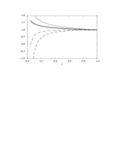
Figure 24: Evolution of renormalization-group-improved potential coefficients in vNRQCD (black lines) and fixed order coefficients (gray lines) for $\nu<1$ in the $t\bar{t}$ system.

The results show the evolution of the potential coefficients in vNRQCD for the $t\bar{t}$ system. For the $b\bar{b}$ system the results are similar. The results in pNRQCD agree for the $1/m^{2}$ potentials, but disagree for the Coulomb and the $1/(m|{\mathbf{k}}|)$ potential. On the horizontal scale of Fig. 24 there is no notable numerical difference between the Coulomb coefficient in vNRQCD (${\cal V}_{c}^{(s)}$) and the corresponding expression in pNRQCD, see Eqs. (102) and (103). In the fixed order approach the ratios simply reduce to $\alpha_{s}^{2}(Mv)/\alpha_{s}^{2}(M)$ for the $\tilde{V}_{k}$ potential (upper gray line) and to $\alpha_{s}(Mv)/\alpha_{s}(M)$ for all the other potentials (lower gray line). The curve for $\alpha_{s}(Mv)/\alpha_{s}(M)$ is on top of the solid line that displays the running of ${\cal V}_{c}^{(s)}(\nu)/{\cal V}_{c}^{(s)}(1)$. This shows that the contributions in the three-loop anomalous dimension of ${\cal V}_{c}^{(s)}(\nu)$ that are induced by the ultrasoft corrections are quite small for the $t\bar{t}$ system.

We find that the evolution in the fixed order and the renormalization-group-improved approach roughly agrees for the Coulomb coefficient and for the $\tilde{V}_{\delta}$ potential. Up to small corrections, both evolve basically with the QCD $\beta$-function. For the $\tilde{V}_{k}$ and the $\tilde{V}_{r}$ potentials, however, the evolution of the fixed order and the renormalization-group-improved coefficients is profoundly different. Whereas the fixed order coefficients grow with $\alpha_{s}$ for smaller scales, the renormalization-group-improved coefficients become smaller. Expanding for example the vNRQCD coefficient ${\cal V}_{k}^{(s)}(\nu)$ in terms of $\alpha_{s}(m)$, we find $\!{}^{{\bf?}}$

$${\cal V}_{k}^{(s)}(\nu) = \Big{(}\frac{C_{F}^{2}}{2}-C_{F}C_{A}\Big{)}\alpha_{s}^{2}(m)-\frac{\beta_{0}}{\pi}\Big{(}\frac{C_{F}^{2}}{2}-C_{F}C_{A}\Big{)}\alpha_{s}^{3}(m)\ln(\nu)$$ (143)

$$-\,\frac{4C_{A}C_{F}(C_{A}+2C_{F})}{3\pi}\>{\alpha_{s}^{3}(m)}\ln(\nu)+\ldots\,.$$

In the expansion of the corresponding fixed order coefficient the order $\alpha_{s}^{3}\beta_{0}$ term agrees, but the third term is missing, because the anomalous dimension of the $\tilde{V}_{k}$ potential is not accounted for properly. Numerically the coefficient of the third term is larger than the coefficient of the second term and has a different sign. This explains the different running for scales below $M$, and leads to a profoundly different behavior of higher order corrections in both approaches.

Currents and Total Cross Section
In the fixed order approach the $Q\bar{Q}$ production currents can be defined in analogy to Eq. (129), see e.g. Refs. [ $\!{}^{{\bf?}}$], and the computation of the correlators ${\cal A}_{1-3}$ follows the lines of Sec. 8.1. Since a consistent summation of higher order QCD logarithms is not intended, the basic requirement is that the regularization scheme used in the solution of the Schrödinger equation in Eq. (126) is also employed in the matching procedure. For the currents $\mbox{\boldmath$O$}_{\mbox{\scriptsize$\mathbf{p}$},2-3}$ Born matching is sufficient. For the dominant current $\mbox{\boldmath$O$}_{\mbox{\scriptsize$\mathbf{p}$},1}$ two-loop matching has to be carried out.

For example, in Ref. [ $\!{}^{{\bf?}}$] a cutoff scheme was used, where the Schrödinger equation in Eq. (126) was solved in a three-dimensional momentum space sphere with radius $\Lambda\sim M$. The coefficient $c_{1}$ was then computed by demanding that the total cross section in NRQCD equals the total cross section in full QCD at order $\alpha_{s}^{2}$ in the limit $\alpha_{s}\ll v\ll 1$. The resulting expression for $c_{1}$ is a complicated function of $M$ and $\Lambda$ and also contains the power counting breaking effects discussed at the end of Sec. 2.2. This matching procedure at the level of the total cross section is called “direct matching” $\!{}^{{\bf?}}$ and also works for ad-hoc regularization schemes that do not have a straightforward definition in mathematical terms. For example in Refs. [ $\!{}^{{\bf?}}$] a cutoff $\Lambda$ was suggested, where the solution of Eq. (126) was expanded for $\Lambda\to\infty$. Logarithmic divergent terms were kept and linear, quadratic, etc. divergences dropped by hand. This scheme was later adopted by all fixed order computations at NNLO except for Refs. [ $\!{}^{{\bf?},{\bf?}}$]. In this scheme also the power counting breaking effects just mentioned are removed by hand. The resulting expression for $c_{1}$ is simpler than in Ref. [ $\!{}^{{\bf?}}$] and has the same order $\alpha_{s}$ contribution as Eq. (74). The scale of $\alpha_{s}$ in $c_{1}$ obtained in this scheme is independent of the scale of $\alpha_{s}$ in the correlators.

9 Top Quark Pair Production at Threshold

Top–antitop quark pair production close to the threshold will provide an integral part of the top quark physics program at the Linear Collider, which is supposed to be the next major accelerator project after the LHC. It is fair to say that top threshold physics was the main motivation for the conceptual and technical progress in heavy quarkonium physics in the recent years. The theoretical interest in the top–antitop quark threshold arises from the fact that the large top quark mass and width ($\Gamma_{t}\approx 1.5$ GeV) lead to a suppression of non-perturbative effects.$\!{}^{{\bf?},{\bf?}}$ Effectively, the top quark velocity is

$$v_{\rm eff}=\left(\frac{\sqrt{s}-2M+2\delta M+i\Gamma_{t}}{M}\right)^{1/2}\,,$$ (144)

so the hierarchy $M_{t}\gg M_{t}|v_{\rm eff}|\gg M_{t}|v_{\rm eff}|^{2}\gg\Lambda_{\rm QCD}$ is satisfied for any energy in the threshold region. This makes top threshold physics an ideal application of the non-relativistic effective theories reviewed in the previous sections. In particular, perturbative methods are a reliable tool to describe the physics of non-relativistic $t\bar{t}$ pairs and allow for measurements of top quark properties directly at the parton level.

Due to the large top width the total $t\bar{t}$ production cross section line shape is a smooth function of the energy, which rises rapidly at the point where the remnant of a toponium 1S resonance can be formed. From the energy where this increase occurs, the top quark mass can be determined, whereas shape and height of the cross section near threshold can be used to determine $\Gamma_{t}$, the coupling strength of top quarks to gluons and, if the Higgs boson is not heavy, the top Yukawa coupling.$\!{}^{{\bf?},{\bf?}}$ For the total top quark width only very few other methods to determine it are known. From differential quantities, such as the top momentum distribution,$\!{}^{{\bf?},{\bf?}}$ the forward–backward asymmetry or certain leptonic distributions,$\!{}^{{\bf?},{\bf?}}$ one can obtain measurements of $\Gamma_{t}$, the top quark spin and possible anomalous couplings.$\!{}^{{\bf?}}$

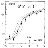
Figure 25: (a) Sensitivity of the $t\bar{t}$ line shape, convoluted by the TESLA $e^{+}e^{-}$ beam luminosity spectrum, to the top quark mass. The solid line corresponds to the nominal mass, while the dotted lines to values which differ from the nominal value by $\pm 200$ and $\pm 400$ MeV. The diagram is taken from an early DESY simulation study in Ref. [ $\!{}^{{\bf?}}$], where the “experimental” points and error bars each correspond to total luminosity of $1$ fb^-1. Theoretical uncertainties are not taken into account. (b) Typical form of the luminosity spectrum at the Linear Collider at nominal beam energy of $350$ GeV due to initial state radiation, beamstrahlung and beam energy spread from Ref. [ $\!{}^{{\bf?}}$].

A considerable number of experimental studies were carried out in the past to assess the feasibility of such measurements.$\!{}^{{\bf?},{\bf?},{\bf?},{\bf?},{\bf?}}$ The measurement of the top quark mass from a threshold line shape scan is particularly interesting, see Fig. 25a for an early simulation study.$\!{}^{{\bf?}}$ In contrast to the standard top mass determination method, which relies on the reconstruction of the invariant mass of jets originating from the decay of a single top quark, the line shape measurement has the advantage that only color-singlet $t\bar{t}$ events have to be counted. Therefore, the effects of final state interactions, uncertainties from hadronization modeling, etc. are suppressed, and systematic uncertainties in the top mass determination are small. Recent simulation studies have shown that, for a total luminosity of $100$ fb^-1, statistical and systematical experimental uncertainties in the top mass determination are well below 50 MeV.$\!{}^{{\bf?},{\bf?}}$ Such a precision would be relevant for example in supersymmetric scenarios, where the lightest CP-even Higgs mass can have a very strong dependence on the top quark mass due to top-stop loops.$\!{}^{{\bf?}}$

9.1 Theoretical Achievements

With the excellent experimental prospect in view it is obvious that a careful analysis and assessment of theoretical uncertainties in the prediction of the total cross section and various distributions is mandatory, in order to determine whether the theoretical precision can meet the experimental one. Initially, a number of leading order $\!{}^{{\bf?}}$ and next-order computations,  $\!{}^{{\bf?},{\bf?},{\bf?},{\bf?},{\bf?},{\bf?}}$ were carried out. The latter relied basically on QCD-inspired potential models that used phenomenological input from $\Upsilon$ and charmonium data. As such they did not represent true first-principles QCD calculations, and there was no systematic way how the computations could be consistently improved to include higher order radiative or relativistic corrections.

After adoption of the concepts of effective theories in the framework of NRQCD (Sec. 2), consistent fixed order NNLO computations appeared in Refs. [ $\!{}^{{\bf?},{\bf?},{\bf?},{\bf?},{\bf?},{\bf?},{\bf?},{\bf?},{\bf?}}$]. The results were not just some new higher order corrections, but led to a number of surprising and important insights. The NNLO corrections to the location where the cross section rises and the height of the cross section were found to be much larger than expected from the results at NLO. The large corrections to the location of the rise were found to be an artifact of the on-shell pole mass definition and it was realized that the top pole mass cannot be extracted with an uncertainty smaller than ${\cal{O}}(\Lambda_{\rm QCD})$ from non-relativistic heavy quark–antiquark systems (Sec. 7). Subsequently, carefully designed threshold mass definitions were suggested to allow for a stable extraction of the top quark mass parameter (Sec. 7). The remaining uncertainties in the normalization of the cross section were estimated $\!{}^{{\bf?}}$ to about $20$% and seemed to jeopardize precise measurements of the top width, the top quark coupling to gluons and the Higgs boson. Some N³LO logarithmic corrections to the cross section were found to be large too $\!{}^{{\bf?},{\bf?}}$ and at present the only way to possibly improve the situation in the fixed order approach seems to be the determination of N³LO corrections in order to learn more about the structure of the perturbative series.

An alternative way is to reorganize the perturbative series by using renormalization-group-improved perturbation theory (Sec. 8.1), which counts $\alpha_{s}\ln v$ of order one and sums all QCD logarithms of $v$ at a certain order into the coefficients of the effective theory. Such a treatment has become standard in many other areas of QCD where physics is governed by widely separated scales. The theoretical framework that allows to carry out such a summation consistently is more sophisticated than NRQCD (Sec. 2). Currently, there are two alternative formulations in the literature, called pNRQCD (Sec. 4) and vNRQCD (Sec. 5). The two effective theories are not equivalent (Sec. 6). Recently, a renormalization-group-improved calculation in vNRQCD of the total cross section at NLL order and including most NNLL order corrections has been provided in Refs. [ $\!{}^{{\bf?}}$]. It was found that the normalization uncertainties are an order of magnitude smaller and the remaining relative uncertainty in the normalization of the cross section was estimated at the level of $3$%.

In the following sections I discuss how the top quark width and non-perturbative effects are implemented into computations of the non-relativistic $t\bar{t}$ dynamics, and I give a more detailed discussion of results for the total cross section in fixed order perturbation theory and the recent results obtained in vNRQCD.

9.2 Top Width and Non-Perturbative Effects in the Total Cross Section

For computations of the total cross section the top width can be understood as a modification of the coefficients of the effective theory caused by electroweak corrections, since one is not interested in the dynamics of the top quark decay. (In general, the top decay would be associated with external currents similarly to the current that produces the $t\bar{t}$ pair.) Because the particles involved in these corrections are lighter than the top quark, they can lead to non-zero imaginary parts in the coefficients of the effective theory. This is a known concept in quantum mechanics of inelastic processes. In the context of top quark threshold production the effects of the top quark decay are the most important part of a whole array of electroweak corrections.

The dominant effect of the top quark width is obtained by including the electroweak top quark selfenergy in the matching conditions for the coefficients of the bilinear top operators. Since the matching is determined for on-shell top quarks, the dominant effect of the top decay is that of an imaginary mass term proportional to the top quark width being added to the effective Lagrangian. For example, in vNRQCD the operators

$$\delta{\cal L}=\sum_{{\mathbf{p}}}\psi_{\mathbf{p}}^{\dagger}\>\frac{i}{2}\Gamma_{t}\>\psi_{\mathbf{p}}\ +\ \sum_{{\mathbf{p}}}\chi_{\mathbf{p}}^{\dagger}\>\frac{i}{2}\Gamma_{t}\>\chi_{\mathbf{p}}\,.$$ (145)

have to be added to the Lagrangian, $\Gamma_{t}$ being the on-shell top decay width. In the Standard Model the dominant decay channel is $t\to bW^{+}$ and gives a width of $\Gamma_{t}=1.43\,{\rm GeV}$ for $m^{t}_{\rm pole}=175$ GeV including one-loop electroweak $\!{}^{{\bf?}}$ (see also Ref. [ $\!{}^{{\bf?}}$]) and two-loop QCD $\!{}^{{\bf?}}$ effects. In the effective theories, $\Gamma_{t}$ is treated as a fixed parameters that can be determined from experiment. Since the typical energy of the top quark is $E\sim M|v_{\rm eff}|^{2}\sim 4\,{\rm GeV}$, it is natural in the Standard Model to count $\Gamma_{t}$ of order $Mv^{2}$. Thus, the propagator of a top quark with momentum $(p^{0},{\mathbf{p}})$ is

$$\frac{i}{p^{0}-\frac{{\mathbf{p}}^{2}}{2M}+\delta M+\frac{i}{2}\Gamma_{t}+i\delta}\,.$$ (146)

In extensions of the Standard Model, where the total top width is different, the $v$-counting might have to be modified. The use of this propagator is equivalent to the replacement $\!{}^{{\bf?}}$ $E\to E+i\Gamma_{t}$ in $t\bar{t}$ Green functions obtained from the Schrödinger equation for stable quarks in Eq. (126), i.e. it is sufficient to replace $v$ by the effective velocity $v_{\rm eff}$ defined in Eq. (144) in the Schrödinger equation of Eq. (126). For the total $t\bar{t}$ cross section the operators in Eq. (145) have been shown to be sufficient to account for all electroweak effects at LO $\!{}^{{\bf?}}$ and NLO $\!{}^{{\bf?}}$ in the fixed order approach. At NNLO the treatment of electroweak effects is more involved, since also first order electroweak corrections to top quark production and decay and background processes consistent with the top decay final state need to be taken into account. The complete set of electroweak effects at NNLO order is currently unknown. However, some one-loop electroweak corrections to the $t\bar{t}$ production current $\!{}^{{\bf?}}$ and some non-resonant background contributions $\!{}^{{\bf?}}$ have been computed. Also, the structure of some higher order effects associated with the electroweak top quark selfenergy is understood. The next order corrections from the selfenergy leads to a top wave function correction in the effective theory, which is up to a different sign equal to the corresponding vertex correction to the gluon-quark coupling contained in the Coulomb potential. In computations of energy levels both contributions cancel due to gauge-invariance. The remaining subdominant width effect arises from the non-relativistic expansion of the top quark spinors of full QCD. In vNRQCD this leads to the following additional operators

$$\delta{\cal L}=-\sum_{{\mathbf{p}}}\psi_{\mathbf{p}}^{\dagger}\>\frac{i}{2}\Gamma_{t}\>\frac{{\mathbf{p}}^{2}}{2M^{2}}\psi_{\mathbf{p}}\ -\ \sum_{{\mathbf{p}}}\chi_{\mathbf{p}}^{\dagger}\>\frac{i}{2}\Gamma_{t}\>\frac{{\mathbf{p}}^{2}}{2M^{2}}\chi_{\mathbf{p}}\,.$$ (147)

Since the effective Lagrangian describes the non-relativistic $t\bar{t}$ dynamics in the center-of-mass frame, these operators can be interpreted as a time-dilatation effect $\sim\Gamma_{t}(1-\langle\frac{{\mathbf{p}}^{2}}{2M^{2}}\rangle+\ldots)$ that arises from the Fermi motion of the individual top quarks in the $t\bar{t}$ system at rest. The cancellation between the electroweak wave function corrections and the electroweak vertex corrections to the Coulomb potential was verified at the one-loop level by explicit calculation in Ref. [ $\!{}^{{\bf?}}$] (see also Ref. [ $\!{}^{{\bf?}}$]). For muonic atoms it was noted before in Ref. [ $\!{}^{{\bf?}}$] and later again in Ref. [ $\!{}^{{\bf?}}$]. An analogous discussion for the $B_{c}$ lifetime can be found in Ref. [ $\!{}^{{\bf?}}$].

The large top quark width plays a crucial role in suppressing the size of non-perturbative hadronic contributions governed by the scale $\Lambda_{\rm QCD}$. Even arbitrarily close to the threshold point, the $t\bar{t}$ system has an effective energy set by the perturbative scale $\Gamma_{t}$, see Eq. (144). For stable quarks, an operator product expansion $\!{}^{{\bf?},{\bf?}}$ in powers of $\Lambda_{\rm QCD}/E$ can be used to incorporate non-perturbative contributions. The first non-perturbative correction arises from the radiation and absorption of a gluon with an energy of order $\Lambda_{\rm QCD}$. In the framework of pNRQCD and in configuration space representation the correction can be understood from the insertion of two ${\mathbf{r}}.{\mathbf{E}}$ interactions, where the gluon field carries no energy and momentum as shown in Fig. 26.

Figure 26: Leading non-perturbative correction in the operator product expansion due to the vacuum average of two chromoelectric fields.

Due to Lorentz and gauge invariance the one-particle-irreducible two-point function of the two chromoelectric fields is related to the vacuum average (or vacuum condensate) of two gluon field strength tensors,

$$\langle 0|E_{i}^{A}E^{B}_{k}|0\rangle=-\frac{1}{96}\delta_{ik}\delta^{AB}\langle 0|G_{\mu\nu}^{C}G^{\mu\nu\,C}|0\rangle\,.$$

The resulting leading correction to the color singlet Green function of the Schrödinger equation in configuration space representation reads $\!{}^{{\bf?}}$

$$\delta G_{s}({\mathbf{r}},{\mathbf{r}}^{\prime}) = -\frac{\pi}{18}\langle 0|\alpha_{s}\,G_{\mu\nu}G^{\mu\nu}|0\rangle\,\int\!d^{3}{\mathbf{x}}\,\int\!d^{3}{\mathbf{y}}\,{\mathbf{x}}.{\mathbf{y}}\,G_{s}({\mathbf{r}},{\mathbf{x}})G_{o}({\mathbf{x}},{\mathbf{y}})G_{s}({\mathbf{y}},{\mathbf{r}}^{\prime})\,,$$

where $G_{o}$ stands for the Green function of the Schrödinger equation with the octet Coulomb potential. For $t\bar{t}$ production the relative size of the gluon condensate correction is of order $[\Lambda_{\rm QCD}/(E+i\Gamma_{t})]^{4}\times v_{\rm eff}^{2}\sim 10^{-4}$. The first factor arises for dimensional reasons and the second term from the ${\mathbf{p}}.{\mathbf{A}}/M$ interaction that comes from the multipole expansion. The radiation of the gluon off the potential (Fig. 3) gives the same estimate. An explicit expression for the gluon condensate corrections to the correlator ${\cal A}_{1}$ was derived in Ref. [ $\!{}^{{\bf?}}$],

$$\delta{\cal A}_{1}(v_{\rm eff},M,\nu)\,=\,\frac{9\,i\,C_{F}^{2}\,\alpha_{s}^{2}}{8\,M^{2}\,v_{\rm eff}^{7}}\,\,\langle 0|\alpha_{s}\,G_{\mu\nu}G^{\mu\nu}|0\rangle\,$$ (149)

$$\qquad\times\,\sum_{n=0}^{\infty}\,\frac{\Gamma(n+4)\Gamma^{2}(n-\lambda)}{(n+2+\frac{\lambda}{8})\Gamma(n+1)\Gamma^{2}(n+5-\lambda)}\hskip 28.45274pt$$

where $\lambda=-C_{F}\alpha_{s}/(2v_{\rm eff})$ and $\Gamma$ is the gamma function. The size of this correction for the (conservative) literature value $\langle 0|\alpha_{s}\,G_{\mu\nu}G^{\mu\nu}|0\rangle=0.05\pm 0.03\,\mbox{GeV}^{4}$ is consistent with the previous parametric estimate and can be safely neglected in view of the current perturbative uncertainties. It is a quite interesting question, whether this estimate of the size of non-perturbative corrections is indeed correct.

9.3 Cross Section at NNLO in the Fixed Order Approach

In the fixed order approach NNLO computations of the $t\bar{t}$ cross section close to threshold in $e^{+}e^{-}$ annihilation have been carried out by Hoang et al., $\!{}^{{\bf?},{\bf?}}$ Melnikov et al., $\!{}^{{\bf?}}$ Yakovlev, $\!{}^{{\bf?}}$ Beneke et al., $\!{}^{{\bf?}}$ Nagano et al., $\!{}^{{\bf?}}$ and Penin et al. $\!{}^{{\bf?}}$ Penin et al. $\!{}^{{\bf?}}$ have also provided a NNLO computation of the $t\bar{t}$ cross section in $\gamma\gamma$ collisions. Since the fixed order computations basically use NRQCD as the conceptual framework (Sec. 2), which does not fix a preferred convention for the regularization of UV divergences, the results obtained by the various groups are, partly, quite different. The differences of the results in the various conventions and regularization schemes can be interpreted as differences in the treatment of corrections from beyond NNLO and serve as an important tool to estimate the inherent uncertainties in the fixed order approach.

In Ref. [ $\!{}^{{\bf?}}$] Hoang et al. solved the momentum space Schrödinger equation in Eq. (126) exactly for the Coulomb potential based on the numerical routines of Ref. [ $\!{}^{{\bf?}}$]; the other $1/m$ suppressed contributions where calculated with time-ordered perturbation theory using a momentum cutoff keeping only terms that depend logarithmically on the cutoff and discarding terms that depend linearly, quadratically, etc. on the cutoff. In Ref. [ $\!{}^{{\bf?}}$] Hoang et al. solved the complete NNLO Schrödiner equation exactly in a momentum sphere with radius $\Lambda\sim M$. In Ref. [ $\!{}^{{\bf?}}$] Melnikov et al. solved the NNLO Schrödinger equation exactly in configuration space representation for the Green function $G(0,r_{0})$, where the distance $r_{0}$ served as the cutoff parameter. They also kept only terms that a logarithmically dependent on $r_{0}$ and discarded power-like divergences. The method was also employed by Yakovlev in Ref. [ $\!{}^{{\bf?}}$] and Nagano et al. in Ref. [ $\!{}^{{\bf?}}$]. A similar regularization method was employed by Penin et al in Refs. [ $\!{}^{{\bf?}}$], but the entire Schrödinger equation was solved with time-ordered perturbation theory supplemented by partial resummations to avoid multiple energy poles. All methods used the direct matching procedure $\!{}^{{\bf?}}$ to determine the coefficient $c_{1}$ of the dominant $t\bar{t}$ production current. The results obtained in these cutoff schemes had a residual dependence on three different scales, the renormalization scale $\mu$ of $\alpha_{s}$ in the potentials, the cutoff and the renormalization scale of $\alpha_{s}$ in the coefficient $c_{1}$. A different strategy was used by Beneke et al. in Refs. [ $\!{}^{{\bf?}}$]. They used dimensional regularization identifying the contributions from the various momentum regions in Eq. (21), i.e. potentials, coefficients, etc., using the threshold expansion and solving the Schrödinger equation in time-ordered perturbation theory. In this approach the potentials and coefficients were determined without an explicit matching calculation. The result had a residual dependence on two different scales, the renormalization scale $\mu$ of $\alpha_{s}$ in the potentials, and the factorization scale. In addition, a summation of some NLL order logarithms was included in $c_{1}$. The prescription used for this summation, however, is not consistent with the known NLL order anomalous dimensions in pNRQCD or vNRQCD. In addition, $c_{1}$ was not included as a global factor of the correlator ${\cal A}_{1}$ but expanded out.

In Ref. [ $\!{}^{{\bf?}}$] the results for the normalized total photon-induced cross section $Q_{t}^{2}R^{v}=\sigma(e^{+}e^{-}\to\gamma\to t\bar{t})/\sigma_{\rm pt}$ of all groups were compiled and compared numerically in detail using an equivalent set of parameters to analyze the scheme-dependence of the fixed order approach. Since the axial-vector current contributions are only a small correction at the few percent level it is justified to consider only the photon-induced cross section. Figure 27 shows the results obtained in Ref. [ $\!{}^{{\bf?}}$] in the pole mass scheme for $m_{\rm pole}=175.05$ GeV, $\alpha_{s}(M_{Z})=0.119$, $\Gamma_{t}=1.43$ GeV and $\mu=15,30$ and $60$ GeV. The other scales where fixed at $M_{\rm pole}$. The effects of the luminosity spectrum of the $e^{+}e^{-}$ beams, which leads to a smearing of the line shape, were not taken into account.

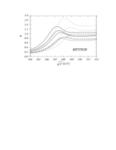
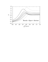
Figure 27: The total normalized photon-induced $t\bar{t}$ cross section $R$ at the Linear Collider versus the c.m. energy in the threshold regime at LO (dotted curves), NLO (dashed) and NNLO (solid) in the pole mass scheme for $m_{t}^{\rm pole}=175.05$ GeV, $\alpha_{s}(M_{Z})=0.119$ , $\Gamma_{t}=1.43$ GeV and $\mu=15$, $30$, $60$ GeV. The plots were given in Ref. [ $\!{}^{{\bf?}}$] from results provided by Hoang-Teubner (HT), Melnikov-Yelkhovsky-Yakovlev-Nagano-Ota-Sumino (MYYNOS), Penin-Pivovarov (PP) and Beneke-Signer-Smirnov (BSS).

Since the method used by Melnikov et al., Yakovlev et al. and Nagano et al. were equivalent, a single figure is displayed for their results. The result of Hoang and Teubner was based on the momentum sphere method of Ref. [ $\!{}^{{\bf?}}$] and has the smallest variations. In particular, the LO result and the NLO and NNLO corrections are smaller than for the other groups. The results in Fig. 27 demonstrate the instability of the “peak position” in the pole mass scheme and the necessity of using threshold masses. It was concluded in Ref. [ $\!{}^{{\bf?}}$] that the perturbative uncertainty in an extraction of the pole mass parameter from the peak position (i.e. when the beam smearing effects are neglected) is around $300$ MeV. The results in Fig. 27 also show a large uncertainty in the normalization of the cross section. This uncertainty is particularly puzzling, because there is no obvious physical reason for its existence. At present it does not seem to be related to renormalon-type higher order corrections, although it has also been speculated that the large size of the corrections could have some infrared origin.$\!{}^{{\bf?}}$ On the other hand, it has been shown in Ref. [ $\!{}^{{\bf?}}$] that the dominant N³LO logarithmic corrections to the cross section of (relative) order $\alpha_{s}^{3}\ln^{2}v$ are at the level of $10$% and not small. It was estimated in Ref. [ $\!{}^{{\bf?}}$] that the present theoretical relative uncertainty in the normalization of the cross section in the fixed order approach is around $20$%.

In Ref. [ $\!{}^{{\bf?}}$] it was also studied how well the peak position can be stabilized, when threshold mass schemes are employed (Sec. 7.2). Figure 28 shows the results for the photon induced total cross section obtained in Ref. [ $\!{}^{{\bf?}}$]

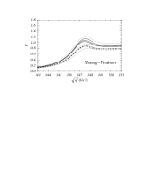
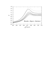
Figure 28: The total normalized photon-induced $t\bar{t}$ cross section $R$ at the Linear Collider versus the c.m. energy in the threshold regime at LO (dotted curves), NLO (dashed) and NNLO (solid) for $\alpha_{s}(M_{Z})=0.119$ , $\Gamma_{t}=1.43$ GeV and $\mu=15$, $30$, $60$ GeV. Hoang–Teubner used the 1S mass $M_{1S}=173.68$ GeV, Melnikov–Yelkhovsky the kinetic $M_{\rm kin}(15~{}\mbox{GeV})=173.10$ GeV, and Beneke–Signer–Smirnov and Yakovlev the PS mass $M_{\rm PS}(20~{}\mbox{GeV})=173.30$ GeV. The plots were given in Ref. [ $\!{}^{{\bf?}}$] from results provided by Hoang–Teubner (HT), Melnikov–Yelkhovsky (MY), Beneke–Signer–Smirnov (BSS) and Yakovlev.

where the respective values of the threshold masses were obtained from the top $\overline{\rm MS}$ mass value $\overline{m}(\overline{m})=165$ GeV as a reference point. Numerically, the series (in an expansion in powers of $\alpha_{s}$ for $\mu=\overline{m}$) that relate the pole mass and the threshold masses used in Fig. 28 to the $\overline{\rm MS}$ mass are as follows: $\!{}^{{\bf?}}$

$$m_{\rm pole} = [\,165+7.64+1.64+0.52+0.25^{(*)}\,]~{}\mbox{GeV}$$

$$M_{\rm 1S} = [\,165+7.21+1.24+0.23+0.05^{(*)}\,]~{}\mbox{GeV}$$

$$M_{\rm PS}(20~{}\mbox{GeV}) = [\,165+6.72+1.21+0.29+0.08^{(*)}\,]~{}\mbox{GeV}$$

$$m_{\rm kin}(15~{}\mbox{GeV}) = [\,165+6.68+1.15+0.27^{(*)}\,]~{}\mbox{GeV}\,.$$ (150)

The numbers indicated by the superscript $(*)$ are estimated in the large-$\beta_{0}$ approximation and $\alpha_{s}(M_{Z})=0.119$ (which corresponds to $\alpha_{s}(165~{}\mbox{GeV})=0.1091$ using four-loop running) has been used. The order $\alpha_{s}^{3}$ terms for the threshold masses are about a factor two smaller than for the pole mass. The results shown in Fig. 28 demonstrate that the peak position is significantly stabilized when threshold masses are employed. It was concluded in Ref. [ $\!{}^{{\bf?}}$] that the perturbative uncertainty in the determination of threshold masses from the peak position (i.e. when beam smearing effects are neglected), is between $50$ and $80$ MeV. It was also pointed out that the $\overline{\rm MS}$ mass can be determined with a comparable perturbative precision, only if $\alpha_{s}(M_{Z})$ is known with an uncertainty of around $0.001$. This restriction arises from the relatively large order $\alpha_{s}$ correction in the relation between threshold masses and $\overline{\rm MS}$ mass. For example, for a given measurement of the 1S mass, let’s say $M_{\rm 1S}=175$ GeV$\,\pm\,\delta M_{\rm 1S}$, and $\alpha_{s}(M_{Z})=0.118\pm x\,0.001$ the result for $\overline{m}(\overline{m})$ reads $\!{}^{{\bf?}}$

$$\overline{m}(\overline{m}) = \bigg{[}\,175-7.58\,-\,0.96\,-\,0.23\,\,\pm\,\delta M_{1S}\,\pm\,x\,0.07\,\bigg{]}~{}\mbox{GeV}\,\qquad$$ (151)

where the first four numbers represent the perturbative series.

The results in Fig. 28 also show that the threshold masses do not affect the normalization of the cross section; the uncertainty of around $20$% remains in threshold mass schemes. This can be understood from the fact that the transfer from the pole mass to threshold masses corresponds predominantly to a shift in the threshold point. The large normalization uncertainties could have severe consequences for experimental measurements. For the measurement of the top quark mass it is conceivable that, after the luminosity spectrum of a specific collider design is folded into the calculations for the cross section, the resulting “peak-less” line-shape (see Fig. 25a) could lead to a transfer of normalization uncertainties into the top mass measurement. In general, such beam effects are smaller for $\mu^{+}\mu^{-}$ colliders, because beamstrahlung is suppressed by the muon mass, see e.g. Ref. [ $\!{}^{{\bf?}}$]. On the other hand, the large normalization uncertainties would make precise measurements of $\alpha_{s}$, $\Gamma_{t}$ or the top quark Yukawa coupling to the Higgs, $y_{t}$ impossible. In the fixed order approach, effects of a Standard Model Higgs can be implemented by a Higgs potential $\tilde{V}_{\rm tth}=-y_{t}^{2}/[2({\mathbf{q}}^{2}+m_{h}^{2})]$ and a correction to the coefficient $c_{1}$.$\!{}^{{\bf?},{\bf?}}$ For a light Higgs they are typically at the level of several percent. Figure 31 shows the variation of the theoretical total cross section $\sigma(e^{+}e^{-}\to\gamma,Z\to t\bar{t}$) for changes in the input parameters $\alpha_{s}$, $\Gamma_{t}$ and $y_{t}$.

The question how well the top mass and the strong coupling can be determined from a threshold scan in $e^{+}e^{-}$ collisions with the TESLA-LC design $\!{}^{{\bf?}}$ was addressed by Peralta et al. $\!{}^{{\bf?}}$ in a simulation study based on the theoretical NNLO calculations for the cross section from Hoang et al. in Ref. [ $\!{}^{{\bf?}}$]. The theoretical computations from Ref. [ $\!{}^{{\bf?}}$] have the smallest theoretical variations of all NNLO computations, so the estimates for the theoretical uncertainties obtained in the experimental study of Ref. [ $\!{}^{{\bf?}}$] are likely to be larger, if the NNLO computation of the other groups are used in a similar analysis. However, the results of Ref. [ $\!{}^{{\bf?}}$] illustrate very well the dependence of the measurements on theoretical uncertainties. In the simulation Peralta et al. included the TESLA luminosity sprectrum and realistic assumptions on efficiencies, background and other systematics. In the study nine scan points were placed onto the $t\bar{t}$ line shape similar to Fig. 25a and a tenth scan point was placed well below the threshold to evaluate the background. At each point an integrated luminosity of $10$ fb^-1 was spent.

                                 

Figure 29: (a) Results of a two-parameter ($M$–$\alpha_{s}(M_{Z})$) $\chi^{2}$ fit ($\Delta\chi^{2}=1$) for the pole, 1S and PS ($\mu_{\rm PS}=20$ GeV) masses using the same NNLO theoretical cross section ($\mu=25$ GeV) for “experiment” and theory. The ellipses show the experimental errors. (b) Result for a two-parameter $M_{\rm 1S}$–$\alpha_{s}(M_{Z})$ $\chi^{2}$ fit ($\Delta\chi^{2}=1$) using different theoretical cross sections for the “experiment” while keeping the theory fixed to NNLO with $\mu=25$ GeV. The shifts in the locations of the ellipses show the theoretical errors. The analysis was carried out in Ref. [ $\!{}^{{\bf?}}$] based on the computations in Ref. [ $\!{}^{{\bf?}}$].

For a two-parameter fit of top mass and $\alpha_{s}(M_{Z})$ Peralta el al. found the correlations shown in Fig. 29a. The error ellipses correspond to $\Delta\chi^{2}=1$. Because the corrections to the ${}^{3}S_{1}$ toponium ground state mass are zero in the 1S scheme, the correlation is smallest for the 1S mass leading to the smallest experimental uncertainties. The experimental uncertainty is $40$ MeV ($50$ MeV) for $M_{\rm 1S}$ ($M_{\rm PS}(20~{}\mbox{GeV})$) and $120$ MeV for the pole mass. The correlation is larger in the pole mass scheme. In order to test the impact of the theoretical uncertainties in the normalization of the cross section the fits were repeated for “experimental” data generated from the LO, NLO and NNLO theoretical predictions and for three different values of the renormalization scale, $\mu=15,25,60$ GeV. The difference in the location of the ellipses are a measure for the theoretical uncertainties; see Fig. 29b for the result in the 1S scheme ($\Delta\chi^{2}=1$). For $M_{\rm 1S}$ and $M_{\rm PS}(20~{}\mbox{GeV})$ the theoretical uncertainties were found to be at the level of $10$–$40$ MeV, whereas the error in $\alpha_{s}(M_{Z})$ was 0.013, which is several times larger then the current world average. For the pole mass the theoretical uncertainty was found to be about $100$ MeV, and the error in $\alpha_{s}(M_{Z})$ was 0.012. This result shows that in a two-parameter fit the large normalization uncertainties of the total cross section are fed almost entirely into $\alpha_{s}$ and essentially leave the measurement of threshold mass parameters unaffected.

Peralta et al. $\!{}^{{\bf?}}$ also carried out a constraint fit taking $\alpha_{s}(M_{Z})=0.120\pm 0.001$ as an input. Here it was found that the experimental uncertainties for $M_{\rm 1S}$, $M_{\rm PS}(20~{}\mbox{GeV})$ and the pole mass are slightly smaller than in the two-parameter fit, but that the theoretical uncertainties for the masses are about $3$–$4$ time larger. This behavior can be understood from the correlation between masses and $\alpha_{s}$ shown in Fig. 29a and from the fact that the large normalization uncertainties of the total cross section are partly absorbed into the mass for a constraint fit.

In a more recent simualtion study by Martinez $\!{}^{{\bf?}}$ the size of the experimental uncertainties for simultaneous measurements of the $1S$ mass, $\alpha_{s}(M_{Z})$, $\Gamma_{t}$ and $y_{t}$ in a top threshold run at an $e^{+}e^{-}$ Linear Collider was reexamined taking into account “data” on total cross section, top three-momentum distribution and forward-backward asymmetry for a 9+1 point threshold scan using a total integrated luminosity of $300$ fb^-1. The intention was to determine which experimental uncertainties could be eventually achieved, and not to estimate theoretical uncertainties. Fixing $y_{t}$ to the Standard Model (SM) value Martinez et al. obtained $\Delta M_{\rm 1S}=18$ MeV, $\Delta\alpha_{s}(M_{Z})=0.0012$ and $\Delta\Gamma_{t}=30$ MeV from a three-parameter fit. In a one parameter fit, fixing all other parameters, they obtained $\delta y_{t}/y_{t}$ between $12$ and $24$%. In a fit where $\Gamma_{t}$ is fixed to the SM value and $\alpha_{s}$ is constrained to $\alpha_{s}(M_{Z})=0.120\pm 0.001$ they obtained $\delta M_{\rm 1S}=25$ MeV and $\delta y_{t}/y_{t}=(+0.31,-0.49)$. In a fit where only $\alpha_{s}$ is constrained to $\alpha_{s}(M_{Z})=0.120\pm 0.001$ they obtained $\delta M_{\rm 1S}=30$ MeV, $\delta\Gamma_{t}=33$ MeV and $\delta y_{t}/y_{t}=(+0.33,-0.57)$ for a Higgs mass of $m_{h}=120$ GeV. For simulation studies for $\mu^{+}\mu^{-}$ colliders see for example Ref. [ $\!{}^{{\bf?}}$].

At present it appears questionable whether the experimental precision for measurements of $\alpha_{s}$, $\Gamma_{t}$ and $y_{t}$ can be matched by the precision of the theoretical computations in the fixed order approach.

9.4 Cross Section at NNLL Order in vNRQCD

At present there exists only one computation of the total $t\bar{t}$ production cross section close to threshold in the renormalization-group-improved approach by Hoang et al. $\!{}^{{\bf?}}$ in the framework of vNRQCD. Since $c_{1}$ does not run and the Coulomb potential evolves trivially with $\alpha_{s}$ at LL order, the LL cross section in the renormalization-group-improved approach and the LO fixed order cross section are equivalent. The NLL cross section in vNRQCD and the NLO fixed order cross section differ because $c_{1}$ runs non-trivially at NLL order. Thus the NLL order cross section and the fixed order NLO cross section differ by a normalization factor. At NNLL order all relevant coefficients for potentials and currents run non-trivially, and the difference to the fixed order NNLO results can be significant with respect to the normalization as well as to the shape of the cross section. Hoang et al. $\!{}^{{\bf?}}$ determined the cross section at LL, NLL and NNLL order. The NNLL order result is incomplete, since it does not include the three-loop evolution of $c_{1}$, which is presently unknown.

In Refs. [ $\!{}^{{\bf?}}$] the calculations were carried out in $D=4-2\epsilon$ dimensions in the $\overline{\rm MS}$ scheme. The Schrödinger equation in Eq. (126) has been solved exactly with numerical methods for all Coulombic contributions, and the corrections from the kinetic energy term ${\mathbf{p}}^{4}/(4M^{3})$ and the $1/m$-suppressed potentials were determined in time-independent perturbation theory.

Figure 30: (a) Normalized photon-induced cross section $Q_{t}^{2}R^{v}$ at LL (dotted lines), NLL (dashed lines) and NNLL (solid lines) order for $M_{\rm 1S}=175$ GeV, $\alpha_{s}(M_{Z})=0.118$, $\Gamma_{t}=1.43$ GeV and $\nu=0.1,0.125,0.2,0.4$ at each order. (b) Total NNLL order cross section in units of pb for the same parameters. The dotted, dashed, dot-dashed, and solid curves correspond to $\nu=0.1,0.15,0.2,0.4$. The figures were obtained with renormalization-group-improved perturbation theory in Ref. [ $\!{}^{{\bf?}}$] using vNRQCD.

In Fig. 30a the normalized photon-induced cross section obtained in Ref. [ $\!{}^{{\bf?}}$] is displayed at LL (dotted lines), NLL (dashed lines) and NNLL (solid lines) order in the 1S mass scheme for $M_{\rm 1S}=175$ GeV and four different choices of the velocity scaling parameter, $\nu=0.1,0.125,0.2,0.4$. The peak position is stable due to the use of a threshold mass scheme. In contrast to the fixed order computations discussed in the previous subsection an excellent convergence of the normalization and a decreasing sensitivity to changes in $\nu$ at higher orders is observed. It was shown that this behavior is a consequence of the evolution of the vNRQCD coefficients, which sum QCD logarithms of $v$ if $\nu$ is chosen of order $v\sim\alpha_{s}$. In particular, the non-trivial evolution of the potential coefficients (Fig. 24) leads to a partial cancellation of NNLL order corrections because some coefficients develop a relative sign difference when $\nu$ is lowered. Such a behavior does not exist at NNLO in the fixed order approach, where all coefficients scale trivially with $\alpha_{s}$ and grow in the same relative direction when the scale $\mu$ is lowered. In Fig. 30b the total NNLL order $t\bar{t}$ cross section including $\gamma$ and $Z$ exchange in units of pb determined in Refs. [ $\!{}^{{\bf?}}$] is displayed for $\nu=0.1,0.15,0.2,0.4$.

From the size of the NNLL order corrections,the $\nu$-variation of the the cross section and an examination of some known higher order corrections, Hoang et al. estimated the remaining perturbative uncertainty of the normalization of the cross section as $3$%, which is a reduction by almost an order of magnitude with respect to estimates in the fixed order approach. If the uncertainty of the renormalization-group-improved approach is established, the prospects for the size of theoretical uncertainties in measurements of top mass, $\alpha_{s}$, $\Gamma_{t}$ and the Yukawa coupling $y_{t}$ from a top threshold scan are significantly better than in the fixed order approach. In particular, for fits where the top couplings are fixed, the danger that the perturbative normalization uncertainties are fed into the top mass measurement is avoided. On the other hand, measurements of $\alpha_{s}$, $\Gamma_{t}$ and $y_{t}$ with acceptable theoretical uncertainties appear only to be possible in the renormalization-group-improved approach.

                          

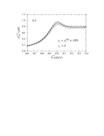
Figure 31: Variation of the NNLL cross section in vNRQCD [ $\!{}^{{\bf?}}$] without beam effects for a) the value of the strong coupling, b) the top quark width, and c) the inclusion of a Standard Model (SM) Higgs boson. Changes relative to the central value (solid lines) are shown by dashed red lines. In c) there are two solid lines, the lower black line is the decoupling limit for the Higgs boson, and the upper blue line is for a SM Higgs with mass $m_{H}=115\,{\rm GeV}$. The parameters $M_{\rm 1S}=175$ GeV, $\Gamma_{t}=1.43$ GeV, $\alpha_{s}(M_{Z})=0.118$, $y_{t}=0$ and $\nu=0.15$ have been used unless stated otherwise.

In Figs. 31 the variation of the NNLL cross section $\sigma_{\rm tot}^{\gamma,Z}$ obtained in Ref. [ $\!{}^{{\bf?}}$] is displayed as a function of $\sqrt{s}$ for different choices of the input parameters $\alpha_{s}(M_{Z})$, $\Gamma_{t}$ and $y_{t}$. In all figures the parameters $M_{\rm 1S}=175$ GeV, $\Gamma_{t}=1.43\,{\rm GeV}$, $\alpha_{s}(M_{Z})=0.118$, $y_{t}=0$ and $\nu=0.15$ are chosen, unless stated otherwise. The upper left panel shows the cross section for $\alpha_{s}(M_{Z})=0.116$ (lower dashed red line), $0.118$ (solid black line), and $0.120$ (upper dashed red line). At the peak one finds a $\pm 2.7\%$ variation when varying $\alpha_{s}(M_{Z})$ by $\pm 0.002$. The upper right panel shows the cross section for $\Gamma_{t}=1.43$ GeV (solid black line). The dashed red lines correspond to variations of $\Gamma_{t}$ by $\pm 10\%$, where for a smaller width the peak becomes more pronounced. At the peak one finds a $(-2.3\%,+2.6\%)$ variation of the cross section when varying $\Gamma_{t}$ by $\pm 5\%$. Finally, the lower panel shows the cross section for zero Yukawa coupling (solid black line), the Standard Model value for the Yukawa coupling (solid blue line), and a $\pm 20\%$ variation of the coupling with respect to the SM value (upper/lower dashed red lines). The Higgs mass was chosen to be $m_{H}=115$ GeV. At the peak one finds a $(+3.3\%,-2.6\%)$ variation when varying $y_{t}^{\rm SM}$ by $\pm 20\%$. For $m_{H}=130$ and $150\,{\rm GeV}$ the corresponding variations are $(+2.9\%,-2.3\%)$ and $(+2.5\%,-2.0\%)$ respectively. Thus, given that the remaining theoretical uncertainty in the normalization of the cross section is $3$%, measurements with theoretical uncertainties $\delta\alpha_{s}(M_{Z})\sim 0.002$, $\delta\Gamma_{t}/\Gamma_{t}\sim 5\%$ and $\delta y_{t}/y_{t}\sim 20\%$ appear feasible. These uncertainties match quite well the estimated experimental uncertainties from a recent simulation study by Martinez $\!{}^{{\bf?}}$ (see end of Sec. 9.3).

10 Bottom Mass from $\Upsilon$ Sum rules

The determination of the Cabibbo-Kobayashi-Maskawa (CKM) matrix elements is one of the main goals of current B physics experiments. A sufficiently accurate determination of the size of the CKM matrix elements and their relative phases will lead to a better understanding of the origin of CP violation, the structure of the weak interaction, and, possibly, to the establishment of physics beyond the Standard Model. For the extraction of the CKM matrix elements from inclusive B decay rates, such as of $V_{cb}$ from the semileptonic decays into $D$ mesons or of $V_{ub}$ from semileptonic decays into light hadrons, an accurate and precise knowledge of the bottom quark mass is desirable due to the strong dependence of the total decay rate on the bottom quark mass parameter (Sec. 7.2).

Non-relativistic sum rules for the masses and electronic decay widths of $\Upsilon$ mesons, bottom-antibottom quark bound states with ${}^{2s+1}L_{j}={}^{3}S_{1}$, are an ideal tool to determine the bottom quark mass: using causality and global duality arguments one can relate integrals over the total cross section for the production of hadrons containing a bottom-antibottom quark pair in $e^{+}e^{-}$ collisions to derivatives of the vacuum polarization function of bottom quark currents at zero-momentum transfer. The $n$-th derivative is referred to as the $n$-th moment of the total cross section. For a particular range of $n$ the moments are dominated by the experimental data on the $\Upsilon$ mesons and, at the same time, can be calculated reliably using perturbative QCD in the non-relativistic expansion. Because the moments have, for dimensional reasons, a strong dependence on the bottom quark mass, $P_{n}\sim 1/M^{2n}$, these sum rules can be used to determine the bottom quark mass to high precision. Within the last few years there have been several analyses at NLO and NNLO in the non-relativistic expansion in the fixed order approach. Initially, the bottom pole mass was extracted, $\!{}^{{\bf?},{\bf?},{\bf?},{\bf?}}$ whereas later analyses $\!{}^{{\bf?},{\bf?},{\bf?},{\bf?}}$ determined threshold mass parameters and the $\overline{\rm MS}$ mass $\overline{m}(\overline{m})$. For an application of non-relativistic sum rules to the $\psi$ family for an extraction of the charm quark mass see Ref. [ $\!{}^{{\bf?}}$].

10.1 Basic Theoretical Issues and Experimental Data

The sum rules for the $\Upsilon$ mesons start from the correlator of two electromagnetic vector currents of bottom quarks at momentum transfer $q$,

$$\Pi(q^{2}) = -\,i\int dx\,e^{i\,q.x}\,\langle\,0\,|\,T\,j^{v}_{\mu}(x)\,j^{v\,\mu}(0)\,|\,0\,\rangle\,.$$ (152)

The $n$-th moment $P_{n}$ of the vacuum polarization function is defined as

$$P_{n}\,\equiv\,\frac{4\,\pi^{2}\,Q_{b}^{2}}{n!}\,\bigg{(}\frac{d}{dq^{2}}\bigg{)}^{n}\,\frac{\Pi(q^{2})}{q^{2}}\bigg{|}_{q^{2}=0}\,,$$ (153)

where $Q_{b}=-1/3$ is the electric charge of the bottom quark. Due to causality the $n$-th moment $P_{n}$ can also be written as a dispersion integral

$$P_{n}\,=\,Q_{b}^{2}\,\int\limits^{\infty}_{s_{\rm min}}\frac{ds}{s^{n+1}}\,R^{v}(s)\,,$$ (154)

where

$$Q_{b}^{2}\,R^{v}(s)\,=\,\frac{\sigma(e^{+}e^{-}\to\gamma\to\mbox{$b\bar{b}$+X})}{\sigma_{\rm pt}}\,=\,\frac{4\,\pi\,Q_{b}^{2}}{s}\,\mbox{Im}\,\Pi(s)$$ (155)

is the total normalized photon-induced cross section of bottom quark–antiquark production in $e^{+}e^{-}$ annihilation. The lower limit of the integration in Eq. (154) is set by the mass of the lowest-lying $b\bar{b}$ resonance. Assuming global duality, the moments $P_{n}$ can be either calculated from experimental data on $R$ or theoretically using perturbative QCD.

The experimental moments $P_{n}^{\rm ex}$ are determined by using the data on the $\Upsilon$ meson masses, $M_{\rm kS}$, and $e^{+}e^{-}$ partial widths, $\Gamma_{\rm kS}$, for $k=1,\ldots,6$, see Ref. [ $\!{}^{{\bf?}}$]. The formula that is used for the experimental moments has the typical form

$$P_{n}^{\rm ex} = \frac{9\,\pi}{\tilde{\alpha}^{2}_{\rm em}}\,\sum\limits_{k=1}^{6}\,\frac{\Gamma_{\rm kS}}{M_{\rm kS}^{2n+1}}\,+\,\int\limits_{s_{{\rm B}\bar{\rm B}}}^{\infty}\frac{ds}{s^{n+1}}\,r_{\rm cont}(s)\,,$$ (156)

and is based on the narrow width approximation for the known $\Upsilon$ resonances; $\tilde{\alpha}_{\rm em}$ is the electromagnetic coupling at the scale $10$ GeV. Because the difference in the electromagnetic coupling for the different $\Upsilon$ masses is negligible, one can chose $10$ GeV as the scale of the electromagnetic coupling for all resonances. Since the continuum cross section above the ${\rm B}\bar{\rm B}$ threshold is quite poorly known experimentally a number of different methods to estimate it has been used in the literature. Usually it is approximated by some theoretically motivated model, based on the perturbative predictions for the continuum region. For very low values of $n\mathrel{\raise 1.29167pt\hbox{$<$\kern-7.5pt\lower 4.30554pt\hbox{$\sim$}}}4$ the uncertainties in the knowledge of the continuum cross section are a significant contribution in the uncertainties of the bottom mass extractions. For $n\mathrel{\raise 1.29167pt\hbox{$>$\kern-7.5pt\lower 4.30554pt\hbox{$\sim$}}}4$ the continuum contribution is suppressed sufficiently so that only a rough estimate of the continuum region is needed. Here, it is sufficient to assume that $r_{c}$ is a constant compatible with the perturbative predictions. In Tab. 1 a compilation is given of the experimental numbers for the $\Upsilon$ resonances needed in Eq. (156).

nS	$M_{\rm nS}/[\mbox{GeV}]$		$\Gamma_{\rm nS}/[\mbox{keV}]$
1S	$\hskip 17.07182pt9$.	$460$	$1.32\pm 0.04\pm 0.03$
2S	$10$.	$023$	$0.52\pm 0.03\pm 0.01$
3S	$10$.	$355$	$0.48\pm 0.03\pm 0.03$
4S	$10$.	$58$	$0.25\pm 0.03\pm 0.01$
5S	$10$.	$86$	$0.31\pm 0.05\pm 0.07$
6S	$11$.	$02$	$0.13\pm 0.03\pm 0.03$

Table 1: The experimental numbers for the $\Upsilon$ masses and electronic decay widths used for the calculation of the experimental moments $P_{n}^{\rm ex}$. For the widths, the first error is statistical and the second one systematic. All errors are estimated from the numbers presented in Refs. [ $\!{}^{{\bf?},{\bf?}}$]. The electromagnetic coupling at $10$ GeV and the ${\rm B}\bar{\rm B}$ threshold point are $\tilde{\alpha}_{\rm em}^{-1}=\alpha_{\rm em}^{-1}(10\,\mbox{GeV})=131.8(1\pm 0.005)$ and $(\sqrt{s})_{{\rm B}\bar{\rm B}}=2\times 5.279$ GeV. The errors in the $\Upsilon$ masses and the ${\rm B}\bar{\rm B}$ threshold $(\sqrt{s})_{{\rm B}\bar{\rm B}}$ are small and can be neglected.

A reliable computation of the theoretical moments $P_{n}^{\rm th}$ based on perturbative QCD is only possible if the effective energy range contributing to the integration in Eq. (154) is sufficiently larger than $\Lambda_{\rm QCD}\sim 300$ MeV.$\!{}^{{\bf?}}$ For large values of $n$ the theoretical moments are dominated by the non-relativistic kinematic regime close to the $\Upsilon$ resonances, and it can be shown that the size of the energy range is proportional $M/n$. This implies that $n$ should be chosen sufficiently smaller than $15$–$20$. A practical upper bound for $n$ is $10$, which has been used in Refs. [ $\!{}^{{\bf?},{\bf?},{\bf?},{\bf?}}$]. Larger values for $n$ up to $20$ have been used in the analyses of Refs. [ $\!{}^{{\bf?},{\bf?},{\bf?},{\bf?}}$]. One argument in favor of using also values of $n$ larger than $10$ is that the leading order gluon condensate contribution of the large-$n$ theoretical moments $\!{}^{{\bf?},{\bf?}}$ (see Fig. 26 and Eq. (LABEL:condensate1)),

$$P_{n}^{\tiny<G^{2}>} = -\frac{\pi\,n^{3}}{72\,M^{4}}\,e^{-0.4C_{F}\alpha_{s}\sqrt{n}}\,\langle 0|\alpha_{s}\,G_{\mu\nu}G^{\mu\nu}|0\rangle\,P^{\rm p.t.}_{n}\,+\,\ldots\,,\qquad$$ (157)

where the $P_{n}^{\rm p.t.}$ is the $n$’s moment obtained from perturbation theory, is less then a percent even for $n<20$. On the other hand, the estimate of non-perturbative effects based on a local expansion in gluonic and light quark condensates is only reliable if $M/n\gg\Lambda_{\rm QCD}$, see Ref. [ $\!{}^{{\bf?}}$]. In addition, the size of the non-perturbative corrections coming from the dimension-$6$ (and higher) condensates as well as all perturbative Wilson coefficients for the condensates are not well known. It has also been argued recently that the condensates might actually not be the dominant non-perturbative effects.$\!{}^{{\bf?}}$

In order to suppress uncertainties from non-perturbative corrections, $n$ should be chosen as small as possible. If $n$ is chosen very small, typically $n\mathrel{\raise 1.29167pt\hbox{$<$\kern-7.5pt\lower 4.30554pt\hbox{$\sim$}}}4$, the dynamics of the $b\bar{b}$ pair encoded in the moments is dominated by relativistic energies and momenta of order $M$, and the usual perturbative expansion in the number of loops can be employed to determine the theoretical moments. At present the normalized photon-induced heavy quark pair production cross section including the full mass dependence is known at two-loop order.$\!{}^{{\bf?}}$ Very few analyses in terms of low-$n$ moments exist in the literature. A recent analysis in terms of low-$n$ moments and extracting the bottom $\overline{\rm MS}$ mass as $\overline{m}(\overline{m})=4.21\pm 0.05$ GeV was carried out in Ref. [ $\!{}^{{\bf?}}$]. Since this review concentrates on non-relativistic dynamics, no discussion on this method can given here. It should be noted that the result from Ref. [ $\!{}^{{\bf?}}$] is consistent with the large-$n$ sum rule analyses that used threshold masses (see Tab. 2).

The strategy that has been employed most frequently in the literature is to use $n$ as large as possible in order to suppress the contribution from the $b\bar{b}$ continuum. Here, $n$ can already been considered large for $n\mathrel{\raise 1.29167pt\hbox{$>$\kern-7.5pt\lower 4.30554pt\hbox{$\sim$}}}4$. The experimental uncertainties for large-$n$ extractions of the bottom mass are around $15$ MeV. In this case, theoretical uncertainties dominate and there is the chance to reduce the uncertainties in the bottom mass extractions by theoretical considerations. In large-$n$ moments the $b\bar{b}$ dynamics is dominated by non-relativistic physics and it is necessary to sum the Coulomb singularities $(\alpha_{s}/v)^{i}$ in the cross section (see Eqs. (125) and (140)). Because the size of the energy range contributing to the $n$-th moment is of order $M/n$, the typical center-of-mass velocity of the bottom quarks in the $n$-th moment is of order $v_{n}=1/\sqrt{n}$. This counting rule allows for a quantitative formulation of the two requirements for the choice of $n$: theoretical reliability demands $Mv_{n}^{2}\gg\Lambda_{\rm QCD}$, and dominance of the non-relativistic dynamics demands $v_{n}\ll 1$. If both requirements are met, the $b\bar{b}$ dynamics encoded in the moments is non-relativistic and perturbative, i.e. the hierarchy $M\gg Mv_{n}\gg Mv_{n}^{2}\gg\Lambda_{\rm QCD}$ is valid and the moments can be computed with the effective theory methods described in the previous section. Thus, from the conceptual point of view there is only a quite narrow window of $n$ values between about $4$ and $10$ that should be used for large-$n$ sum rules. If these considerations are applied to $c\bar{c}$ systems, there is no window of $n$ values left for which a sum rule analysis based on non-relativistic moments can be justified.

At present only fixed order analyses have been carried out for the large-$n$ $\Upsilon$ sum rules. Initially the bottom pole mass was determined. After the relevance of the bad high order behavior of the pole mass for $Q\bar{Q}$ systems was fully appreciated and suitable threshold mass schemes were proposed (Sec. 7), subsequent analyses extracted threshold masses, which were in a second step converted to the $\overline{\rm MS}$ mass $\overline{m}(\overline{m})$. In the following I give a historically ordered compilation of the various sum rule analyses including brief descriptions of the respective methods. The main results that have been given by the authors are collected in Tab. 2. In Tab. 2 I have also collected bottom quark mass results from $b\bar{b}$ sum rules not discussed in this review and from perturbative computations of the $\Upsilon(\mbox{1S})$ mass (Sec. 11.2). The results are compatible to recent lattice analyses (see Refs. [ $\!{}^{{\bf?}}$] and references therein) and the measurements from three-jet rates a LEP. $\!{}^{{\bf?}}$ It should be noted that the uncertainties obtained from recent lattice analyses have uncertainties that are comparable to the ones obtained from the perturbative analyses discussed in this review. However, the lattice numbers for $\overline{m}(\overline{m})$ generally tend towards larger values. $\!{}^{{\bf?}}$

author	$\overline{m}_{b}(\overline{m}_{b})$	other mass	comments, Ref.
Voloshin 95		$m_{\rm pole}=4.83\pm 0.01$	NLO $\Upsilon$ sum rules, no theo.uncert. [ $\!{}^{{\bf?}}$]
Kühn 98		$m_{\rm pole}=4.78\pm 0.04$	NLO $\Upsilon$ sum rules [ $\!{}^{{\bf?}}$]
Penin 98		$m_{\rm pole}=4.78\pm 0.04$	NNLO $\Upsilon$ sum rules [ $\!{}^{{\bf?}}$]
Hoang 98		$m_{\rm pole}=4.88\pm 0.13$	NLO $\Upsilon$ sum rules [ $\!{}^{{\bf?}}$]
Hoang 98	$4.26\pm 0.09$ *	$m_{\rm pole}=4.88\pm 0.09$	NNLO $\Upsilon$ sum rules [ $\!{}^{{\bf?}}$]
Melnikov 98	$4.20\pm 0.10$	$M^{1\mbox{\tiny GeV}}_{\rm kin}=4.56\pm 0.06$	NNLO $\Upsilon$ sum rules [ $\!{}^{{\bf?}}$]
Penin 98	$4.21\pm 0.11$ *	$m_{\rm pole}=4.80\pm 0.06$	NNLO $\Upsilon$ sum rules [ $\!{}^{{\bf?}}$]
Jamin 98	$4.19\pm 0.06$		$\Upsilon$ sum rules; no exact info [ $\!{}^{{\bf?}}$]
Hoang 99	$4.20\pm 0.06$	$M_{\rm 1S}=4.71\pm 0.03$	NNLO $\Upsilon$ sum rules [ $\!{}^{{\bf?}}$]
Beneke 99	$4.26\pm 0.09$	$M^{2\mbox{\tiny GeV}}_{\rm PS}=4.60\pm 0.11$	NNLO $\Upsilon$ sum rules [ $\!{}^{{\bf?}}$]
Hoang 00	$4.17\pm 0.05$	$M_{\rm 1S}=4.69\pm 0.03$	NNLO $\Upsilon$ sum rules, charm mass eff. [ $\!{}^{{\bf?}}$]
Kühn 01	$4.21\pm 0.05$		low-$n$ $\Upsilon$ sum rules, ${\cal O}(\alpha_{s}^{2})$ [ $\!{}^{{\bf?}}$]
Pineda 97		$m_{\rm pole}=5.00^{+0.10}_{-0.07}$	NNLO $\Upsilon(\mbox{1S})$ mass & non-pert. eff. [ $\!{}^{{\bf?}}$]
Beneke 99	$4.24\pm 0.09$	$M^{2\mbox{\tiny GeV}}_{\rm PS}=4.58\pm 0.08$	NNLO $\Upsilon(\mbox{1S})$ mass & non-pert. eff. [ $\!{}^{{\bf?}}$]
Hoang 99	$4.21\pm 0.07$	$M_{\rm 1S}=4.73\pm 0.05$	NNLO $\Upsilon(\mbox{1S})$ mass &. non-pert. eff. [ $\!{}^{{\bf?}}$]
Pineda 01	$4.21\pm 0.09$	$M_{\rm RS}^{2\mbox{\tiny GeV}}=4.39\pm 0.11$	NNLO $\Upsilon(\mbox{1S})$ mass & non-pert. eff. [ $\!{}^{{\bf?}}$]
Brambilla 01	$4.19\pm 0.03$		NNLO $\Upsilon(\mbox{1S})$ mass, p.th. only [ $\!{}^{{\bf?}}$]

Table 2: Collection in historical order of results of bottom quark mass determinations from $\Upsilon$ sum rules (upper part) and calculations of the $\Upsilon(\mbox{1S})$ mass (lower part). All results are given in units of GeV and rounded to units of $10$ MeV. Only results where $\alpha_{s}$ was taken as an input are shown. The uncertainties quoted in the respective references have been added quadratically. For analyses with several authors only the respective first author is quoted. The $\overline{\rm MS}$ mass result that are indicated with a star have been determined with an inconsistent conversion formula.

10.2 Pole Mass Results

Extractions of the bottom quark pole mass were carried out at NLO by Voloshin $\!{}^{{\bf?}}$ and by Kühn et al., $\!{}^{{\bf?}}$ and at NNLO by Penin and Pivovarov $\!{}^{{\bf?}}$ and by Hoang.$\!{}^{{\bf?}}$ In this section the methods and results are briefly described. The corresponding values for $\overline{m}(\overline{m})$ are computed from the formula for $m_{\rm pole}/r_{m}$ in Eq. (116). The two-loop relation is used for a NLO sum rule analysis and the three-loop relation for a NNLO sum rule analysis. This order-dependent conversion is necessary to achieve the numerical cancellation of the large infrared-sensitive contributions contained in the pole mass definition (Sec. 7.2). Since in all analyses the information on the exact correlation of the numerical pole mass value with the set of theoretical parameters used for the fits was not quoted, I carry out the conversion treating the pole mass result as uncorrelated. All uncertainties are added quadratically and perturbative conversion uncertainties are included. The values for the $\overline{\rm MS}$ mass obtained from the pole mass in this way needs to be interpreted with some caution, because the full correlation should have been taken into account (Sec. 7.1).

The NLO analysis by Voloshin $\!{}^{{\bf?}}$ was the first large-$n$ sum rule analysis consistent with non-relativistic power counting. Voloshin used time-independent perturbation theory to determine the NLO corrections to the correlator ${\cal A}_{1}$ (Eq. (135)). The moment integration of Eq. (154) was carried out in a strict non-relativistic expansion. After deforming the contour into the complex energy plane away from the bound state poles the integration can be solved using inverse Laplace transformations. This method has the feature that bound state and continuum contributions are treated at the same time and in exactly the same way with respect to the non-relativistic expansion, i.e. the corrections to bound state energies in the energy denominators of the resonances are also expanded. For each moment Voloshin set the scale $\mu$ in the Coulomb potential such that the NLO correction to the Green function vanishes. The scale of $\alpha_{s}$ in $c_{1}$ (Eqs. (133)) was set to the bottom mass. He carried out a two parameter $\chi^{2}$ fit for $m_{\rm pole}$ and $\alpha_{s}$ using four moments $P_{n}$ ($n=8,12,16,20$) and obtained $m_{\rm pole}=4.827\pm 0.007$ MeV and $\alpha_{s}(M_{Z})=0.109\pm 0.001$. The result does not account for perturbative uncertainties. Using Voloshin’s value for $\alpha_{s}$ the corresponding $\overline{\rm MS}$ mass, and two-loop conversion, gives $\overline{m}(\overline{m})=4.33\pm 0.01$ GeV. For $\alpha_{s}(M_{Z})=0.118\pm 0.003$ one obtains $\overline{m}(\overline{m})=4.27\pm 0.04$ GeV.

Voloshin’s NLO analyses was repeated by Kühn, Penin and Pivovarov (KPP) in Ref. [ $\!{}^{{\bf?}}$] and Hoang in Ref. [ $\!{}^{{\bf?}}$]. KPP used time-independent perturbation theory for ${\cal A}_{1}$ and solved the moment integration exactly in the form of Eq. (154). This method treats bound state and continuum contributions differently, because the bound state energy corrections in the energy denominators of the resonances are not expanded out. KPP also improved the convergence of the perturbative series by absorbing some part of the higher order corrections in the Coulomb potential into the LO Coulomb charge. KPP fitted individual moments for $10\leq n\leq 20$ taking $\alpha_{s}(M_{Z})=0.118$ as an input. The scale of $\alpha_{s}$ in $c_{1}$ was set equal to $\mu$, the scale in the LO Coulomb potential. They obtained $m_{\rm pole}=4.78\pm 0.04$ GeV, where the uncertainty was estimated from the variation of the result with $n$, $\mu=1.2$–$4.8$ GeV and when the NNLO corrections to the Coulomb potential in the Schrödinger equation are included. For the corresponding $\overline{\rm MS}$ mass, using the two-loop relation, one obtains $\overline{m}(\overline{m})=4.18\pm 0.05$ GeV for $\alpha_{s}(M_{Z})=0.118\pm 0.003$.

Hoang $\!{}^{{\bf?}}$ used Voloshin’s method to determine the NLO moments, but did not fix $\mu$. He carried out $\chi^{2}$ fits using moments for various sets of $n$’s in the range between $4$ and $10$ for a given value of $\mu$. Perturbative uncertainties were estimated by repeating the fit many times choosing random values for $\mu$ between $1.5$ and $3.5$ GeV and for the scale of $\alpha_{s}$ in $c_{1}$ between $2.5$ and $10$ GeV. In a two-parameter fit he obtained $m_{\rm pole}=4.78\pm 0.14$ GeV and $\alpha_{s}(M_{Z})=0.109\pm 0.023$. The result for the pole mass corresponds to $\overline{m}(\overline{m})=4.18\pm 0.13$ GeV at the two-loop level for $\alpha_{s}(M_{Z})=0.118\pm 0.003$ as an input. Taking $\alpha_{s}(M_{Z})$ as an input Hoang obtained $m_{\rm pole}=4.88\pm 0.13$ GeV for $\alpha_{s}(M_{Z})=0.118\pm 0.004$. This corresponds to $\overline{m}(\overline{m})=4.28\pm 0.13$ GeV at the two-loop level for $\alpha_{s}(M_{Z})=0.118\pm 0.003$.

In the first NNLO analyses by Penin and Pivovarov (PP) $\!{}^{{\bf?}}$ and the NNLO analysis by Hoang $\!{}^{{\bf?}}$ time-independent perturbation theory was used to determine the NNLO corrections to the correlators. The UV-divergences were regularized with a cutoff and the two-loop corrections to $c_{1}$ were determined using the direct matching method.$\!{}^{{\bf?}}$ The moment integration and the fitting procedure were equivalent to the respective methods by PP and Hoang in their NLO analyses. PP improved the convergence as in Ref. [ $\!{}^{{\bf?}}$] and fitted individual moments for $10\leq n\leq 20$ taking $\alpha_{s}(M_{Z})=0.118$ as an input. The scale of $\alpha_{s}$ in $c_{1}$ and the cutoff scale were set equal to $\mu$, the scale of $\alpha_{s}$ in the LO Coulomb potential. They obtained $m_{\rm pole}=4.78\pm 0.04$ GeV, where the uncertainty was estimated from the varying $n$ and the scale $\mu=m_{\rm pole}\pm 1$ GeV. In order to determine $\overline{m}(\overline{m})$ from this NNLO pole mass result one now has to use the three-loop relation for $n_{\ell}=4$ massless quarks. For $\alpha_{s}(M_{Z})=0.118\pm 0.003$ one obtains $\overline{m}(\overline{m})=4.05\pm 0.07$ GeV.

In his NNLO analysis Hoang $\!{}^{{\bf?}}$ carried out $\chi^{2}$ fits using moments for various sets of $n$’s in the range between $4$ and $10$ for a given value of $\mu$. As in his NLO analysis, perturbative uncertainties were determined from varying independently $\mu$ between $1.5$ and $3.5$ GeV, and the scale in $\alpha_{s}$ in $c_{1}$ and the cutoff between $2.5$ and $10$ GeV. In a two-parameter fit Hoang obtained $m_{\rm pole}=4.83\pm 0.07$ GeV and $\alpha_{s}(M_{Z})=0.110\pm 0.014$. The pole mass value corresponds to $\overline{m}(\overline{m})=4.10\pm 0.09$ GeV at the three-loop level for $\alpha_{s}(M_{Z})=0.118\pm 0.003$. Taking $\alpha_{s}(M_{Z})=0.118\pm 0.004$ as an input he obtained $m_{\rm pole}=4.88\pm 0.09$ GeV, which corresponds to $\overline{m}(\overline{m})=4.14\pm 0.10$ GeV using the three-loop conversion for $\alpha_{s}(M_{Z})=0.118\pm 0.003$. For the determination of the $\overline{\rm MS}$ mass Hoang used the two-loop relation and obtained $\overline{m}(\overline{m})=4.26\pm 0.09$ GeV for the two-parameter fit and $\overline{m}(\overline{m})=4.24\pm 0.08$ GeV, if $\alpha_{s}$ is taken as an input. In both cases Hoang accounted for the correlation between $m_{\rm pole}$ and $\alpha_{s}(M_{Z})$ obtained from the fitting.

In the second NNLO analysis by PP $\!{}^{{\bf?}}$ the methods from their first analysis were used, but $\mu$ was varied between $3.5$ and $6.5$ GeV and moments for $n$ between $8$ and $12$ were employed. In this analysis PP obtained $m_{\rm pole}=4.80\pm 0.06$ GeV, taking $\alpha_{s}(M_{Z})=0.118$ as an input. For $\alpha_{s}(M_{Z})=0.118\pm 0.003$ this result corresponds to $\overline{m}(\overline{m})=4.06\pm 0.08$ GeV if the proper three-loop relation is used. PP used the two-loop relation and obtained $\overline{m}(\overline{m})=4.21\pm 0.11$ GeV.

10.3 Threshold Mass Results

Extractions of threshold masses at NNLO were carried out by Melnikov and Yelkhovsky, $\!{}^{{\bf?}}$ Hoang $\!{}^{{\bf?},{\bf?}}$ and Beneke and Signer.$\!{}^{{\bf?}}$ In this section the methods and results of the respective analyses are briefly described.

In the analysis by Melnikov and Yelkhovsky (MY) $\!{}^{{\bf?}}$ the kinetic mass $M_{\rm kin}(1~{}\mbox{GeV})$ was determined. The theoretical moments were determined in time-independent perturbation theory in the pole mass scheme using the same methods as previous NNLO analyses. The moment integration was carried out in the form Eq. (154) and the energy denominators of the bound state resonances were not expanded out. MY fitted individual moments for $n=14,16,18$ taking $\alpha_{s}(M_{Z})=0.118$ as an input and extracted the bottom pole mass as a correlated parameter for a given choice of $\mu$ between $2$ and $4.5$ GeV. The scale of $\alpha_{s}$ in $c_{1}$ and the cutoff were fixed to $5$ GeV. For each value of $\mu$ MY determined subsequently the kinetic mass using the numerical value for $\mu$ for which the pole mass value was determined. To achieve the numerical cancellation of the large infrared-sensitive corrections it was important to keep the bound state energy denominators unexpanded. In Tab. 3 the results obtained by MY for $\mu$ between $2$ and $4.5$ GeV are displayed.

$$\begin{array}[]{||c||c||c|c||c|c||c|c||}\hline\cr&&\vrule\lx@intercol\hfil 14\hfil\lx@intercol\vrule\lx@intercol&\vrule\lx@intercol\hfil 16\hfil\lx@intercol\vrule\lx@intercol&\vrule\lx@intercol\hfil 18\hfil\lx@intercol\vrule\lx@intercol\\ \cline{3-8}\cr{\rm Scales}&{\rm Order~{}of~{}PT}&m_{\rm pole}&M_{\rm kin}&m_{\rm pole}&M_{\rm kin}&m_{\rm pole}&M_{\rm kin}\\ \hline\cr\hline\cr\mu=4.5~{}{\rm GeV}&{\rm LO}&4.69&4.57&4.7&4.57&4.7&4.575\\ \cline{2-8}\cr\mu_{c_{1}}=5~{}{\rm GeV}&{\rm NLO}&4.74&4.49&4.75&4.50&4.76&4.51\\ \cline{2-8}\cr\Lambda=5~{}{\rm GeV}&{\rm NNLO}&4.89&4.51&4.90&4.52&4.91&4.53\\ \hline\cr\hline\cr\mu=3.5~{}{\rm GeV}&{\rm LO}&4.73&4.59&4.73&4.59&4.73&4.595\\ \cline{2-8}\cr\mu_{c_{1}}=5~{}{\rm GeV}&{\rm NLO}&4.77&4.50&4.78&4.511&4.79&4.52\\ \cline{2-8}\cr\Lambda=5~{}{\rm GeV}&{\rm NNLO}&4.95&4.54&4.96&4.55&4.96&4.55\\ \hline\cr\hline\cr\mu=2.5~{}{\rm GeV}&{\rm LO}&4.79&4.63&4.79&4.63&4.79&4.63\\ \cline{2-8}\cr\mu_{c_{1}}=5~{}{\rm GeV}&{\rm NLO}&4.82&4.505&4.83&4.517&4.84&4.525\\ \cline{2-8}\cr\Lambda=5~{}{\rm GeV}&{\rm NNLO}&5.08&4.595&5.08&4.595&5.09&4.6\\ \hline\cr\hline\cr\mu=2~{}{\rm GeV}&{\rm LO}&4.84&4.67&4.84&4.666&4.84&4.66\\ \cline{2-8}\cr\mu_{c_{1}}=5~{}{\rm GeV}&{\rm NLO}&4.84&4.49&4.85&4.505&4.86&4.514\\ \cline{2-8}\cr\Lambda=5~{}{\rm GeV}&{\rm NNLO}&5.21&4.66&5.21&4.66&5.21&4.66\\ \hline\cr\end{array}$$

Table 3: The bottom quark pole mass and the kinetic mass $M_{\rm kin}(1~{}\mbox{GeV})$ in units of GeV for $\mu$ between $2$ and $4.5$ GeV obtained by Melnikov and Yelkhovsky in Ref. [ $\!{}^{{\bf?}}$] for the moments $n=14,16,18$.

MY found pole mass values in the range between $4.5$ and $5.2$ GeV, where the NNLO shifts were larger than the NLO one. For the kinetic mass the results were more stable in the range between $4.49$ and $4.67$ GeV. However, the NNLO shifts were still quite large compared to the NLO ones. For $\mu=4.5$ the convergence is quite good, but for $\mu=2$ GeV the NNLO and NLO shifts are of equal size. Since the resulting series for $m_{\rm kin}(1~{}\mbox{GeV})$ is alternating, MY argued heuristically that the convergence could be improved by an Euler transformation on the series. In this way they obtained the result

$$M_{\rm kin}(1~{}\mbox{GeV})\,=\,4.56\,\pm\,0.06~{}\mbox{GeV}\,,$$

which is somewhat between the NLO and NNLO values and has an uncertainty that is smaller than the range covered by the NLO and NNLO values obtained in the analysis. Since the kinetic mass is a short-distance mass there is no conceptual need to convert the result to the $\overline{\rm MS}$ mass at a particular order. In general, one should go for the best (i.e. highest order) conversion. MY determined the $\overline{\rm MS}$ mass at two-loop order and obtained $\overline{m}(\overline{m})=4.20\pm 0.10$ GeV.

In the analysis by Hoang $\!{}^{{\bf?}}$ the 1S mass was determined. The theoretical moments were computed directly in the 1S mass scheme using time-independent perturbation theory and the methods of Ref. [ $\!{}^{{\bf?}}$] (Sec. 10.2). All NLO and NNLO corrections in the Schrödinger equation in Eq. (126) were strictly treated perturbatively, i.e. the cancellation of the large infrared-sensitive corrections associated with the pole mass were eliminated analytically. For the fitting procedure exactly the same method was used as for the earlier pole mass analysis in Ref. [ $\!{}^{{\bf?}}$]. Hoang carried out $\chi^{2}$ fits using various sets of $n$’s in the range between $4$ and $10$. For all moments in a given set the same value of $\mu$ was chosen. This fitting procedure is different from fits of individual moments, because it put highest statistical weight on linear combinations of moments that are the least sensitive to the experimental uncertainties in the electronic partial widths of the $\Upsilon$ mesons. Since the correlation of the experimental moments coming from the $e^{+}e^{-}$ partial widths (see Eq. (156)) is similar to the correlation of the theoretical moments coming from their dependence on the $b\bar{b}$ wave function at the origin, the resulting $\chi^{2}$ function has a smaller sensitivity to variations of $\mu$ than the individual moments. In contrast to fits of individual moments, which exclusively use information on the size of the moments, the $\chi^{2}$ fitting procedure also uses information on the relative size of the moments as a function of $n$. Hoang estimated the perturbative uncertainties by repeating the fit many times choosing independently random values for $\mu$ between $1.5$ and $3.5$ GeV, for the scale of $\alpha_{s}$ in $c_{1}$ and for the cutoff between $2.5$ and $10$ GeV. In a two-parameter fit Hoang obtained $M_{\rm 1S}=4.67\pm 0.07$ GeV and $\alpha_{s}(M_{Z})=0.112\pm 0.023$ at NLO and $M_{\rm 1S}=4.70\pm 0.03$ GeV and $\alpha_{s}(M_{Z})=0.116\pm 0.013$ at NNLO. A graphical representation of the NLO and NNLO fit results is displayed in Fig. 32a and b.

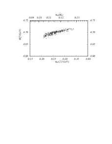
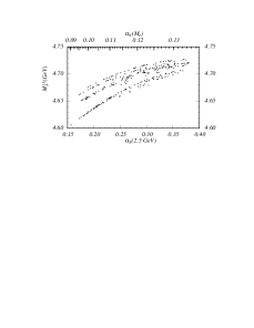
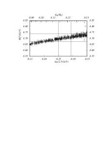
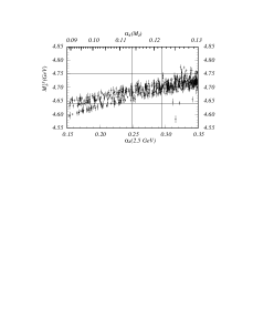
Figure 32: Result for the allowed region in the $M_{\rm 1S}^{b}$-$\alpha_{s}$ plane obtained by Hoang in Ref. [ $\!{}^{{\bf?}}$]. (a) Two parameter fit at NNLO and (b) NLO. The dots represent points of minimal $\chi^{2}$ for a large number of random choices for the scales and sets of $n$’s. Experimental errors are not displayed. (c) Single parameter fit at NNLO and (d) NLO taking $\alpha_{s}$ as an input. The dots represent points of minimal $\chi^{2}$ for a large number of random choices for the scales, sets of $n$’s and $\alpha_{s}$ . Experimental errors at 95% CL are displayed as vertical bars.

In a single parameter fit taking $\alpha_{s}(M_{Z})=0.118\pm 0.004$ as an input Hoang obtained $M_{\rm 1S}=4.70\pm 0.05$ GeV at NLO. At NNLO he obtained

$$M_{\rm 1S}=4.71\pm 0.03~{}\mbox{GeV}\,,$$

which was considered the main result of the analysis. A graphical representation of the NLO and NNLO fit results is displayed in Fig. 32c and d. The results in Fig. 32 show that the 1S mass has a very weak correlation to $\alpha_{s}$. Thus the uncertainty in $\alpha_{s}$ is practically irrelevant for the error in the 1S mass. In contrast to the analysis by Melnikov and Yelkovsky $\!{}^{{\bf?}}$ and later by Beneke and Signer $\!{}^{{\bf?}}$ the results at NLO and NNLO by Hoang are consistent with each other. The range of the NNLO result is contained entirely in the range of the NLO result. This is a consequence of the fitting method used by Hoang. Hoang converted the result to the $\overline{\rm MS}$ mass at two loops using the large-$\beta_{0}$ approximation for the three-loop correction as an estimate for the perturbative uncertainty. He obtained $\overline{m}(\overline{m})=4.20\pm 0.06$ GeV for $\alpha_{s}(M_{Z})=0.118\pm 0.004$. The uncertainty is larger than for the 1S mass because of the perturbative uncertainty in the conversion ($40$ MeV) and the uncertainty in $\alpha_{s}(M_{Z})$ ($40$ MeV), which arises from a relatively large one-loop correction in the relation between 1S and $\overline{\rm MS}$ mass, see Eq. (116). In Ref. [ $\!{}^{{\bf?}}$] Hoang repeated the analysis taking into account also the effects of the non-zero charm quark mass. For $\overline{m}_{c}(\overline{m}_{c})=1.4\pm 0.3$ GeV he obtained

$$M_{\rm 1S}=4.69\pm 0.03~{}\mbox{GeV}$$

for the 1S mass for the same fitting procedure. The result was converted to the $\overline{\rm MS}$ mass using the full three-loop relation leading to $\overline{m}(\overline{m})=4.17\pm 0.05$ GeV for $\alpha_{s}(M_{Z})=0.118\pm 0.003$.

In the analysis by Beneke and Signer (BS) $\!{}^{{\bf?}}$ the PS mass $m_{\rm PS}(2~{}\mbox{GeV})$ was determined. The theoretical moments were computed in the PS mass scheme using time-independent perturbation theory to solve the Schrödinger equation of Eq. (126). BS used dimensional regularization and identified the form of the potentials and coefficients using the threshold expansion, i.e. they did not carry out an explicit matching calculation. The moments of BS depend on $\mu$, the scale of $\alpha_{s}$ and the factorization scale, which was set to the bottom quark mass. The moment integration was solved in the form of Eq. (154), but all NLO and NNLO corrections were strictly treated perturbatively by expanding out the resonance delta functions in $R^{v}$ in order to achieve an explicit analytical cancellation of the large infrared-sensitive corrections associated with the pole mass definition. BS also carried out a summation of some NLL order logarithms in $c_{1}$. The prescription they used, however, is not consistent with the known NLL order anomalous dimensions in pNRQCD or vNRQCD. BS fitted the $n=10$ moment taking $\alpha_{s}(M_{Z})=0.118\pm 0.003$ as an input and varying $\mu$ between $2$ GeV and $2m_{\rm PS}(2~{}\mbox{GeV})/\sqrt{10}$. At NNLO they obtained

$$M_{\rm PS}(2~{}\mbox{GeV})=4.60\pm 0.11~{}\mbox{GeV}\,,$$

where the scale variation is the dominant source of uncertainty ($100$ MeV). The uncertainty from the strong coupling ($30$ MeV) and from the experimental data ($20$ MeV) are small. At NLO BS obtained $m_{\rm PS}(2~{}\mbox{GeV})=4.44$ GeV as the central value with a smaller scale variation. No explicit uncertainties for the NLO result were quoted. A graphical representation of the results is shown in Fig. 33.

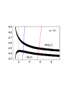
Figure 33: The value of $M_{\rm PS}(2\,\mbox{GeV})$ in units of GeV obtained by Beneke and Signer in Ref. [ $\!{}^{{\bf?}}$] from the 10th moment as a function of the renormalization scale in NLO and NNLO and for $\alpha_{s}(M_{Z})=0.118$. The dark region specifies the variation due to the experimental error on the moment. The two outer lines display the scale variation from which the perturbative error was computed.

Similar to the analysis of Melnikov and Yelkhovsky, which was also based on fits of individual moments, the NLO and NNLO results are not compatible numerically. BS considered the NNLO result given above as the main result of the analysis. The discrepancy with the NLO number was not included in the error estimate. The PS mass at $2~{}\mbox{GeV}$ has a stronger correlation to the input value of $\alpha_{s}(M_{Z})$ than for example the 1S mass. Taking into account this correlation to $\alpha_{s}$ and $\mu$ BS obtained $\overline{m}(\overline{m})=4.26\pm 0.09$ GeV for the $\overline{\rm MS}$ mass using two-loop conversion. The mean value also contains a $-10$ MeV shift from a large-$\beta_{0}$ estimate for the (at the time of the analysis unknown) three-loop correction. The uncertainty from the strong coupling ($10$ MeV) and from the conversion ($20$ MeV) were small. The mean value for the $\overline{\rm MS}$ mass obtained by BS is higher than the one by MY. This is because BS did not take into account their NLO results in the determination of the mean value.

The analyses by MY, Hoang and BS are conceptually equivalent with respect to the computations of the moments in the framework of NRQCD. The differences in the results are a consequence of differences in the fitting methods and the treatment of perturbative uncertainties. Because the uncertainties are dominated by theory, the error estimate is, naturally, a quite delicate task. As such none of the analyses can a priori be considered better or more realistic than another one. Nevertheless, the quoted uncertainties have been subject to controversial discussions, which shall be not repeated in this review. From a (at least for me) conservative point of view it is fair to say all three analyses contain elements that allow to consider the quoted uncertainties as optimistic. The analysis by MY and BS showed that the results for the threshold masses at NLO and NNLO obtained from fits of individual moments are not compatible. MY dealt with this problem by using heuristic arguments on alternating series and BS by ignoring the NLO results in the final result. The origin of the difference between NLO and NNLO results is that the R-ratio that is contained in the moments of Eq. (154) has quite large NNLO corrections. We face this problem also in fixed order computations of the $t\bar{t}$ production cross section close to threshold, which is discussed in Sec. 9.3, see Fig. 28. In the fitting procedure by Hoang the normalization problem of the R-ratio was treated by also using information of the relative size of the moments for different $n$, similar to taking ratios of the moments.

Clearly, the situation is not completely satisfactory and further improvements in the computation of theoretical moments will be necessary to settle the question of the uncertainties in the bottom quark determination from $\Upsilon$ sum rules. One promising path might be to use renormalization-group-improved perturbation theory for the computation of the moments. In the case of top production this has indeed improved the stability of the R-ratio (Sec. 9.4). At the present time a renormalization-group-improved sum rule analysis has not yet been carried out.

11 Heavy Quarkonium Spectrum

Theoretical descriptions of the heavy quarkonium spectrum represent the classic application of non-relativistic quarkonium physics. Early work in QCD-inspired potential models provided very precise determinations of charmonium and bottomonium spectra and physical insights into the long-distance aspects of interquark forces.$\!{}^{{\bf?}}$ However, potential models cannot be derived quantitatively from first principles in QCD, which makes them less suitable for determinations of QCD parameters, most notably the heavy quark masses. With the advent of effective theories for heavy quarkonium systems (Secs. 2, 4, 5) a first principle description of the spectrum has become possible conceptually, but precise computations are difficult, because a reliable technology only exists for systems where the hierarchy $m\gg mv\gg mv^{2}\gg\Lambda_{\rm QCD}$ is valid. This is the case that is discussed generically in Sec. 11.1. In this case the predictions of the effective theories can be computed perturbatively supplemented by local condensate contributions, which incorporate averaged non-perturbative effects. As a matter of principle, at most the bottomonium ground states can be expected to be described with this technology. Determinations of the bottom quark mass from the mass of the $\Upsilon(\mbox{1S})$ state are described in Sec. 11.2. Considerations of the toponium spectrum are irrelevant, due to the large top decay width $\Gamma_{t}\approx 1.5~{}\mbox{GeV}\gg\Lambda_{\rm QCD}$ (see Sec. 9).

For most quarkonium systems $mv^{2}$ is of order $\Lambda_{\rm QCD}$ or even smaller. In the framework of pNRQCD an approach for these systems has been roughly outlined $\!{}^{{\bf?}}$ (Sec. 4.6), but no systematic prescription to carry out quantitative computations of the spectrum has yet been devised. In the framework of vNRQCD such systems can a priori not be treated because ultrasoft modes are by construction already present at the hard matching scale and because soft and ultrasoft scales are correlated at all times (Sec. 5). In the framework of NRQCD (Sec. 2), on the other hand, a systematic treatment of the spectrum of these systems is unknown with analytic methods, but is possible with lattice simulations.$\!{}^{{\bf?}}$ On the lattice, theoretical precision is limited by systematic uncertainties, such as from unquenching and extrapolating and matching to the continuum limit. No further discussion on lattice methods for heavy quarkonium spectra is given in this review. In a recent analysis Brambilla et al. $\!{}^{{\bf?},{\bf?}}$ examined the charmonium, bottomonium and $B_{c}$ spectrum using only the perturbative contributions for the case $m\gg mv\gg mv^{2}\gg\Lambda_{\rm QCD}$. Setting the renormalization scale using a minimal sensitivity prescription they found remarkable agreement of the bottomonium sprectrum up to the $n=3$ radial excitation without accounting for any non-perturbative effects. Brambilla et al. concluded that perturbative methods devised for the case $m\gg mv\gg mv^{2}\gg\Lambda_{\rm QCD}$ might have a wider range of applicability than previously expected. For subsequent discussions following the same interpretation see also Ref. [ $\!{}^{{\bf?}}$]. The results of Brambilla et al., however, appear to be in sharp contradiction to results on the size of non-perturbative corrections obtained for higher bottomonium excitations in Ref. [ $\!{}^{{\bf?}}$].

11.1 Calculation of the $Q\bar{Q}$ Spectrum

For the case $m\gg mv\gg mv^{2}\gg\Lambda_{\rm QCD}$ the computation of the heavy quarkonium spectrum follows the presentation given in Sec. 8 on heavy quark production close to threshold. At NNLL order in the renormalization-group-improved approach of pNRQCD (Sec. 4) or vNRQCD (Sec. 5), or at NNLO in the fixed order NRQCD (Sec. 2) approach the perturbative contribution of $Q\bar{Q}$ dynamics can be described by a common text-book two-body Schrödinger equation. In momentum space representation and in a threshold mass scheme the Schrödinger equation has the generic form

$$\bigg{[}\,\frac{\mathbf{p}^{2}}{M}\bigg{(}1+\frac{\delta M}{M}\bigg{)}-\frac{\mathbf{p}^{4}}{4M^{3}}-(E+2\,\delta M)\,\bigg{]}\,\tilde{\Psi}({\mathbf{p}})$$ (158)

$$\quad\qquad\qquad\qquad\qquad+\int\frac{d^{3}{\mathbf{k}}}{(2\pi)^{3}}\,\tilde{V}({\mathbf{p}},{\mathbf{k}})\,\tilde{\Psi}({\mathbf{k}})=\,0\,.$$

The perturbative contribution of the masses of the $Q\bar{Q}$ states are given by the energy eigenvalues of Eq. (158),

$$M_{Q\bar{Q}}^{\rm\scriptsize pert} = 2M+E\,.$$ (159)

The classification of the solutions according to quantum numbers is standard text-book knowledge and shall not be repeated here. The renormalization-group-improved computation for the energy eigenvalues at NNLL order takes the generic form

$$E = M\alpha_{s}^{2}\,\sum\limits_{i}\left(\alpha_{s}\ln\alpha_{s}\right)^{i}\,\bigg{\{}1\,\mbox{(LL)};\alpha_{s},\,\mbox{(NLL)};\alpha_{s}^{2}\,\mbox{(NNLL)}\bigg{\}}\,.$$ (160)

In the fixed order approach logarithms of $\alpha_{s}$ are not summed and the energy eigenvalues at NNLO have the generic form

$$E = M\alpha_{s}^{2}\,\bigg{\{}1\,\mbox{(LO)};\alpha_{s},\,\mbox{(NLO)};\alpha_{s}^{2}\,\mbox{(NNLO)}\bigg{\}}\,.$$ (161)

In Eq. (158) the difference between renormalization-group-improved and fixed order computation is just the form of the coefficients of the potential $\tilde{V}$ (see Secs. 8.1 and 8.2). From the technical point of view the computations needed to solve Eq. (158) are equivalent in both approaches. In the fixed order approach the first computation of the NNLO $Q\bar{Q}$ spectrum was carried out by Pineda and Yndurain $\!{}^{{\bf?}}$ (see also Refs. [ $\!{}^{{\bf?},{\bf?}}$]). Renormalization-group-improved computations at NNLL order were carried out by Hoang et al. in Ref. [ $\!{}^{{\bf?}}$] and by Pineda in Ref. [ $\!{}^{{\bf?}}$]. Technically, the energy eigenvalues are determined using Rayleigh-Schrödinger time-independent perturbation theory starting from the well known leading order non-relativistic Coulomb solution and including successively higher order terms from the potential and the kinetic energy term. To achieve an explicit cancellation of the unphysical large-order behavior associated with the pole mass it is mandatory to consistently include the contributions of $\delta M$ at each order of perturbation theory (Sec. 7.2). Since at NNLL order (or NNLO) the corresponding integrals do not contain any UV divergences, no regularization prescription for Eq. (158) needs to be specified at this order.

At N³LL order (or N³LO) the computations of the perturbative part of the $Q\bar{Q}$ spectrum becomes more complicated. Apart from N³LL order (or N³LO) corrections to the potential $\tilde{V}$, which include for example two-loop corrections to the $1/m|{\mathbf{k}}|$ potential or three-loop corrections to the Coulomb potential and the corresponding three- and four-loop anomalous dimensions, also non-logarithmic corrections from ultrasoft gluons need to be considered (see for example Figs. 5 and 18). The latter corrections involve UV divergences and depend on the regularization scheme. The corresponding UV divergences are canceled by conterterms of the $1/m^{2}$, $1/m|{\mathbf{k}}|$ and $1/{\mathbf{k}^{2}}$ potentials (Secs. 4.3, 5.7 and 6), which become renormalized. The sum of the ultrasoft corrections and the corrections from the potentials are scheme-independent. The ultrasoft corrections are the QCD analogue of the Bethe-log corrections known from QED and cannot be represented by a two-body Schrödinger equation, because they correspond to a higher Fock $Q\bar{Q}$-Gluon state. Some corrections at N³LO in the fixed order approach are already known. The non-logarithmic corrections from ultrasoft gluons were determined in Ref. [ $\!{}^{{\bf?}}$], and two-loop corrections to the $1/m|{\mathbf{k}}|$ potential were determined in Ref. [ $\!{}^{{\bf?}}$]. The N³LO corrections in the large-$\beta_{0}$ approximation were determined in Refs. [ $\!{}^{{\bf?},{\bf?}}$]. From the NNLL order renormalization-group-improved computations $\!{}^{{\bf?},{\bf?}}$ (see also Ref. [ $\!{}^{{\bf?}}$]) all N³LO corrections proportional to powers of $\ln\alpha_{s}$ are also known. In Ref. [ $\!{}^{{\bf?}}$] Kiyo and Sumino claimed that additional NNLO corrections $\propto M\alpha_{s}^{4}$ and $M\alpha_{s}^{4}\ln\alpha_{s}$ are found when Bethe-Salpeter rather than effective theory techniques are employed with dimensional regularization. The contributions found in Ref. [ $\!{}^{{\bf?}}$] originate from an incomplete expansion of the small $k_{0}$ component of the one-loop corrections to the Coulomb potential in the potential region (Eq. (21)) and are unphysical.

In the case $m\gg mv\gg mv^{2}\gg\Lambda_{\rm QCD}$ the non-perturbative contributions to the spectrum can be expressed as an expansion in terms of local gluon and light quark condensates.$\!{}^{{\bf?},{\bf?}}$ At leading order in the multipole expansion the first non-perturbative correction arises from radiation and absorption of a gluon with energy of order $\Lambda_{\rm QCD}$ from the $Q\bar{Q}$ pair. Conceptually this contribution is closely related to the ultrasoft correction mentioned before. For $mv^{2}\gg\Lambda_{\rm QCD}$, both contributions can be separated by an expansion in $\Lambda_{\rm QCD}/mv^{2}$, see Refs. [ $\!{}^{{\bf?},{\bf?}}$]. Physically, this expansion means that the time span between emission and absorption of the gluon is much smaller than the non-perturbative correlation time. In configuration space representation the coupling of the gluon to the $Q\bar{Q}$ pair is just the ${\mathbf{r}}.{\mathbf{E}}$ interaction in pNRQCD. In momentum space representation the interaction arises from the diagrams in Fig. 3. The first non-perturbative correction is in analogy to Eq. (LABEL:condensate1) and reads $\!{}^{{\bf?},{\bf?}}$

$$E_{nl}^{\rm\scriptsize n.p.} = -\frac{\pi}{18}\,\langle 0|\alpha_{s}G_{\mu\nu}G^{\mu\nu}|0\rangle\,\int\!d^{3}{\mathbf{x}}\,\int\!d^{3}{\mathbf{y}}\,{\mathbf{x}}.{\mathbf{y}}\,\Psi_{nl}({\mathbf{x}})\,G_{o}({\mathbf{x}},{\mathbf{y}})\,\Psi_{nl}({\mathbf{y}})$$ (162)

$$= \frac{8\,\pi\,n^{6}\,M\,a_{nl}}{9\,(MC_{F}\alpha_{s})^{4}}\,\langle 0|\alpha_{s}G_{\mu\nu}G^{\mu\nu}|0\rangle\,,$$

where $a_{1S}=1.652$, $a_{2S}=1.783$, $a_{3S}=1.869$, $a_{2P}=1.123$, etc.. The next order terms in the $\Lambda_{\rm QCD}/mv^{2}$ expansion correspond to dimension-six condensates and have been determined by Pineda in Ref. [ $\!{}^{{\bf?}}$]. It should be noted that the coefficients of the operator expansion in local condensates are at present only known at LO (or LL order) in the non-relativistic expansion and still have a rather large scheme-dependence.

The summation of all orders in $\Lambda_{\rm QCD}/mv^{2}$ leads formally to non-local condensate contributions (see e.g. Refs. [ $\!{}^{{\bf?},{\bf?}}$]) describing the non-perturbative corrections for $\Lambda_{\rm QCD}\sim mv^{2}$. A reliable quantitative treatment of non-perturbative corrections for this case in quarkonium systems has not yet been developed. However, for $\Lambda_{\rm QCD}\sim mv^{2}$ also the perturbative contributions are affected because gluons with ultrasoft energies and energies of order $\Lambda_{\rm QCD}$ are identical and cannot be separated, and because $\alpha_{s}(mv^{2})$ has to be considered of order one. This means that the non-perturbative/ultrasoft corrections have to be counted as NNLO contributions.

11.2 Bottom Mass Determinations from the $\Upsilon(\mbox{1S})$ Mass

There are a number of analyses where the bottom mass was determined from the $\Upsilon(\mbox{1S})$ mass using fixed order calculations at NNLO as described in the previous section. From the technical point of view, in all analyses it was assumed that the hierarchy $m\gg mv\gg mv^{2}\gg\Lambda_{\rm QCD}$ is valid and that non-perturbative corrections can be expressed as an operator expansion in terms of local condensates. The expression for the perturbative contribution of the $\Upsilon(\mbox{1S})$ mass at NNLO in a threshold mass scheme (Sec. 7.2) with $\delta M=M-m_{\rm pole}=\delta M_{\rm LO}+\delta M_{\rm NLO}+\delta M_{\rm NNLO}$ reads ($a_{s}=\alpha_{s}^{(n_{\ell}=4)}(\mu)$)

$$M_{\Upsilon(\mbox{\scriptsize 1S})}^{\mbox{\scriptsize pert}} = 2\,M\,-\,2\,\Big{[}\,M\Delta^{\rm LO}+\delta M_{\rm LO}\,\Big{]}\,-\,2\,\Big{[}\,M\Delta^{\rm NLO}+\delta M_{\rm NLO}\,\Big{]}$$ (163)

$$\hskip 28.45274pt\,-\,2\,\Big{[}\,M\Delta^{\rm NNLO}+\delta M_{\rm NNLO}-\Delta^{\rm LO}\delta M_{\rm LO}\,\Big{]}\,,$$

where, assuming massless light quarks,

$$\Delta^{\rm LO} = \frac{C_{F}^{2}\,a_{s}^{2}}{8}\,,\qquad\Delta^{\rm NLO}\,=\,\frac{C_{F}^{2}\,a_{s}^{2}}{8}\,\Big{(}\frac{a_{s}}{\pi}\Big{)}\,\bigg{[}\,\beta_{0}\,\bigg{(}L+1\,\bigg{)}+\frac{a_{1}}{2}\,\bigg{]}\,,$$

$$\Delta^{\rm NNLO} = \frac{C_{F}^{2}\,a_{s}^{2}}{8}\,\Big{(}\frac{a_{s}}{\pi}\Big{)}^{2}\,\bigg{[}\,\beta_{0}^{2}\,\bigg{(}\,\frac{3}{4}L^{2}+L+\frac{\zeta_{3}}{2}+\frac{\pi^{2}}{24}+\frac{1}{4}\,\bigg{)}+\beta_{0}\,\frac{a_{1}}{2}\,\bigg{(}\,\frac{3}{2}\,L+1\,\bigg{)}$$

$$\hskip 14.22636pt+\frac{\beta_{1}}{4}\,\bigg{(}\,L+1\,\bigg{)}+\frac{a_{1}^{2}}{16}+\frac{a_{2}}{8}+\bigg{(}\,C_{A}-\frac{C_{F}}{48}\,\bigg{)}\,C_{F}\pi^{2}\,\bigg{]}\,,$$

$$L \equiv \ln\Big{(}\frac{\mu}{C_{F}\,a_{s}\,M}\Big{)}\,.$$ (164)

The one- and two-loop coefficients of the beta-function, $\beta_{0}$ and $\beta_{1}$, and the constants $a_{1}$ and $a_{2}$ are from the corrections to the Coulomb potential in Eq. (36). In the 1S mass scheme $\delta M_{\rm LO,NLO}=-M\Delta^{\rm LO,NLO}$ and $\delta M_{\rm NNLO}=-M\Delta^{\rm NNLO}-M(\Delta^{{\rm LO}})^{2}$, and, by construction, perturbative corrections are zero. The non-perturbative contribution from Eq. (162) reads

$$E_{10}^{\rm\scriptsize n.p.} = \frac{0.465\,\pi}{M^{3}\,\alpha_{s}^{4}}\,\langle 0|\alpha_{s}G_{\mu\nu}G^{\mu\nu}|0\rangle\,.$$ (165)

Typical values for the gluon condensate used in the literature are in the range $\langle 0|\alpha_{s}G_{\mu\nu}G^{\mu\nu}|0\rangle=0.05\pm 0.03\,\mbox{GeV}^{4}$. The threshold mass is extracted from fitting $M_{\Upsilon(\mbox{\scriptsize 1S})}^{\mbox{\scriptsize pert}}+E_{10}^{\rm\scriptsize n.p.}$ to the experimental value $\!{}^{{\bf?}}$ $M_{\Upsilon(\mbox{\scriptsize 1S})}^{\mbox{\scriptsize exp}}=9460.30\pm 0.26$ MeV.

In the following I review the bottom mass determinations based on fixed order NNLO calculations in historical order. The results obtained in the analyses are collected in Tab. 2. To simplify the presentation on the determination of uncertainties I discuss only the dominant source of uncertainties as obtained in the different analyses.

Pineda and Yndurain (PY) $\!{}^{{\bf?}}$ determined the pole mass. For the strong coupling PY used a scheme where part of the corrections to the Coulomb potential are absorbed into $\alpha_{s}$. In this scheme the size of the non-perturbative contribution was at the level of $10$ MeV. PY obtained $m_{\rm pole}=5.00^{+0.10}_{-0.07}$ GeV, where the uncertainty was dominated by the error in the strong coupling, $\alpha_{s}(M_{Z})=0.114^{+0.006}_{-0.004}$. PY also determined the $\overline{\rm MS}$ mass using two-loop conversion, $\overline{m}(\overline{m})=4.44^{+0.04}_{-0.03}$ GeV. Converting to the $\overline{\rm MS}$ mass at three loops, which is necessary to achieve the numerical cancellation of the large unphysical corrections associated with the pole mass, the central value reads $\overline{m}(\overline{m})=4.32$ GeV for $\alpha_{s}(M_{Z})=0.114$, using the formula for $m_{\rm pole}/r_{m}$ in Eq. (116).

Hoang $\!{}^{{\bf?}}$ determined the 1S mass. In the 1S scheme there is, by construction, no correlation to $\alpha_{s}$. Perturbative uncertainties cannot be estimated in the usual way by changing the renormalization scale $\mu$. A conservative estimate would be, for example, to account for the difference in the result when $\Delta_{\rm NNLO}$ is replaced by its large-$\beta_{0}$ approximation. Hoang assigned $100$ MeV for the size of the non-perturbative contributions and treated them as an overall uncertainty without including them in the determination of the central value. He obtained $M_{\rm 1S}=4.73\pm 0.05$ GeV. Perturbative uncertainties were not included. Using three-loop conversion to the $\overline{\rm MS}$ mass he obtained $\overline{m}(\overline{m})=4.21\pm 0.07$ GeV for $\alpha_{s}(M_{Z})=0.118\pm 0.004$. The uncertainty is larger than the one of the 1S mass because the $\overline{\rm MS}$ -1S mass relation has a rather strong dependence on $\alpha_{s}$ coming from the one-loop correction in the $\overline{\rm MS}$ -pole mass relation. Since the 1S mass (as well as the PS and the RS mass mentioned below) are short-distance masses the conversion to the $\overline{\rm MS}$ mass does not have to be carried out at a specific order. However, one should go for the highest order conversion to keep perturbative uncertainties small. A compact approximation of the three-loop conversion formula for the $\overline{\rm MS}$ -1S mass relation, which also accounts for charm mass effects and the scale $\mu$ in the strong coupling, was given in Ref. [ $\!{}^{{\bf?}}$],

$$\overline{m}(\overline{m}) = \Big{[}\,4.169\,\mbox{GeV}-0.01\,\Big{(}\overline{m}_{c}(\overline{m}_{c})-1.4\,\mbox{GeV}\Big{)}+0.925\,\Big{(}M_{\rm 1S}-4.69\,\mbox{GeV}\Big{)}$$ (166)

$$\,-9.1\,\Big{(}\alpha_{s}^{(5)}(M_{Z})-0.118\Big{)}\,\mbox{GeV}+0.0057\,\Big{(}\mu-4.69\Big{)}\,\mbox{GeV}\,\Big{]}\,.$$

For $\overline{m}_{c}(\overline{m}_{c})>0.4$ GeV and $\mu>2.5$ GeV the difference between this approximation formula and the exact result is less than $3$ MeV.

Beneke and Signer (BS) $\!{}^{{\bf?}}$ determined the PS mass. They estimated the uncertainty in the PS mass coming from the non-perturbative contributions as $\pm 70$ MeV and obtained $M_{\rm PS}(2~{}\mbox{GeV})=4.58\pm 0.08$ GeV, where non-perturbative contributions were not included in the central value and $\alpha_{s}(M_{Z})=0.118\pm 0.004$ was taken as an input. For the $\overline{\rm MS}$ mass BS used three-loop conversion, and they obtained $\overline{m}(\overline{m})=4.24\pm 0.09$ GeV.

Pineda $\!{}^{{\bf?}}$ determined the RS and RS^′ masses assuming a $75$ MeV uncertainty from the non-perturbative and N³LO ultrasoft contributions. He obtained $M_{\rm RS}(2~{}\mbox{GeV})=4.39\pm 0.11$ GeV and $M_{\rm RS^{\prime}}(2~{}\mbox{GeV})=4.78\pm 0.08$ GeV. The error in the RS mass is significantly larger than the error from the non-perturbative and N³LO ultrasoft contributions due to a theoretical ambiguity in the subtraction term that defines the RS mass. For the $\overline{\rm MS}$ mass he used three-loop conversion, and obtained a combined result of $\overline{m}(\overline{m})=4.21\pm 0.09$ GeV.

Brambilla, Sumino and Vairo (BSV) $\!{}^{{\bf?}}$ determined the $\overline{\rm MS}$ mass directly from the $\Upsilon(\mbox{1S})$ mass without taking into account non-perturbative contributions, which technically means that they used Eq. (166) inserting half the $\Upsilon(\mbox{1S})$ mass as the 1S mass value. They fixed the renormalization scale $\mu$ using a minimal sensitivity requirement, which corresponds to $\mu\approx 2.5$ GeV in Eq. (166). BSV obtained $\overline{m}(\overline{m})=4.19\pm 0.03$ GeV taking $\alpha_{s}(M_{Z})=0.118\pm 0.002$ as an input.

12 Conclusions

In the last few years the conceptual understanding of the perturbative treatment of heavy quarkonium systems with $m\gg mv\gg mv^{2}\gg\Lambda_{\rm QCD}$, $m$ and $v$ being the heavy quark mass and velocity, respectively, has improved considerably. New effective theories have been developed that are more sophisticated than NRQCD and that allow systematic QCD calculations using fixed order or renormalization-group-improved perturbation theory. Starting from solutions of the non-relativistic Schrödinger equation, perturbative corrections can now be computed in dimensional regularization to any order using a fixed set of rules. At the same time, the required technology has been developed to carry out computations at next-to-next-to-leading and higher orders, and the role of the infrared sensitivity of quark mass definitions in the non-relativistic context has been understood. In this review I have tried to give a comprehensive overview of the developments and the applications of the new technologies to bottom quark mass determinations and top quark threshold physics. What comes next?

The main field of application of the new technologies is top quark pair production close to threshold, which is a major part of the top physics program at the Linear Collider. This is because the top mass and the top quark widths are so much larger than the typical hardonization scale. Practically all aspects of the non-relativistic top-antitop dynamics can be described predominantly with perturbative methods based on the new developments. Thus, top threshold measurements will very likely provide the insights into the interplay of perturbative and non-perturbative aspects of QCD one hoped for already after the discovery of $J/\psi$. Still, a lot of work remains to be done to establish the theoretical tools that will make this possible. At present, the new effective theory methods have exclusively been applied to computations of the total cross section, where non-perturbative and electroweak effects are small. The most important outcome of these calculations is that top mass measurements from a threshold scan will have a precision at the level of $100$ MeV, which will be unsurpassed by any other method. But calculations should also be attempted with the same theoretical precision for differential observables. At certain kinematic endpoints the impact of non-perturbative and also electroweak effects can be enhanced. At present, systematic studies of such effects using the new technologies have not yet been carried out. Measured by the progress that already happened in the last few years I am optimistic that developments in this direction will take place in short time.

References

References

- [1] T. Appelquist and H. D. Politzer, Phys. Rev. Lett. 34, 43 (1975); A. De Rujula and S. L. Glashow, Phys. Rev. Lett. 34, 46 (1975); T. Appelquist, A. De Rujula, H. D. Politzer and S. L. Glashow, Phys. Rev. Lett. 34, 365 (1975); T. Appelquist and H. D. Politzer, Phys. Rev. D12, 1404 (1975).
- [2] W. Buchmuller and S. H. Tye, Phys. Rev. D24, 132 (1981).
- [3] K. G. Wilson, Phys. Rev. D10, 2445 (1974).
- [4] M. A. Shifman, A. I. Vainshtein and V. I. Zakharov, Nucl. Phys. B147, 385 (1979); V. A. Novikov, et al. Phys. Rept. 41 (1978) 1.
- [5] M. B. Voloshin, Nucl. Phys. B154, 365 (1979); Yad. Fiz. 35, 1016 (1982) [Sov. J. Nucl. Phys. 35, 592 (1982)]; Yad. Fiz. 36, 247 (1982) [Sov. J. Nucl. Phys. 36,143 (1982)].
- [6] H. Leutwyler, Phys. Lett. B98, 447 (1981).
- [7] H. A. Bethe and E. E. Salpeter, Quantum Mechanics of One- and Two-Electron Atoms, (Academic Press Inc., New York, 1957).
- [8] W. E. Caswell and G. P. Lepage, Phys. Lett. B167, 437 (1986).
- [9] G. T. Bodwin, E. Braaten and G. P. Lepage, Phys. Rev. D51, 1125 (1995) [Erratum-ibid. D55, 5853 (1995)] [hep-ph/9407339].
- [10] S. Fleming, hep-ph/0112058; F. Maltoni, hep-ph/0007003. I. Z. Rothstein, hep-ph/9911276.
- [11] B. A. Thacker and G. P. Lepage, Phys. Rev. D43, 196 (1991).
- [12] A. H. Hoang, Phys. Rev. D56, 5851 (1997) [hep-ph/9704325]; Phys. Rev. D57, 1615 (1998) [hep-ph/9702331].
- [13] A. Pineda and J. Soto, Nucl. Phys. Proc. Suppl. 64, 428 (1998) [hep-ph/9707481].
- [14] M. E. Luke, A. V. Manohar and I. Z. Rothstein, Phys. Rev. D61, 074025 (2000) [hep-ph/9910209].
- [15] M. Beneke and V. A. Smirnov, Nucl. Phys. B522, 321 (1998) [hep-ph/9711391].
- [16] A. V. Manohar, Phys. Rev. D56, 230 (1997) [hep-ph/9701294].
- [17] P. Labelle, Phys. Rev. D58, 093013 (1998) [hep-ph/9608491].
- [18] P. Labelle and S. Mohammad Zebarjad, Can. J. Phys. 77, 267 (1999) [hep-ph/9611313].
- [19] T. Kinoshita and M. Nio, Phys. Rev. D53, 4909 (1996) [hep-ph/9512327]; Phys. Rev. D55, 7267 (1997) [hep-ph/9702218].
- [20] P. Labelle, G. P. Lepage and U. Magnea, Phys. Rev. Lett. 72, 2006 (1994) [hep-ph/9310208]; A. H. Hoang, P. Labelle and S. M. Zebarjad, Phys. Rev. Lett. 79, 3387 (1997) [hep-ph/9707337]; Phys. Rev. A 62, 012109 (2000) [hep-ph/9909495].
- [21] R. Hill and G. P. Lepage, Phys. Rev. D62, 111301 (2000); R. J. Hill, Phys. Rev. Lett. 86, 3280 (2001).
- [22] P. Labelle, Ph.D.Thesis, Cornell University (1994), UMI-94-16736-mc.
- [23] G. P. Lepage, nucl-th/9706029.
- [24] H. Georgi, Phys. Lett. B240, 447 (1990).
- [25] B. Grinstein and I. Z. Rothstein, Phys. Rev. D57, 78 (1998) [hep-ph/9703298].
- [26] M. E. Luke and M. J. Savage, Phys. Rev. D57, 413 (1998) [hep-ph/9707313].
- [27] V. A. Smirnov, Commun. Math. Phys. 134, 109 (1990); Phys. Lett. B394, 205 (1997) [hep-ph/9608151].
- [28] A. Czarnecki and K. Melnikov, Phys. Rev. Lett. 87, 013001 (2001) [hep-ph/0012053].
- [29] A. Czarnecki and K. Melnikov, hep-ph/0110028.
- [30] V. A. Smirnov, Renormalization And Asymptotic Expansions, (Basel, Switzerland: Birkhäuser (1991) 380 p., Progress in physics, 14).
- [31] V. A. Smirnov, Applied Asymptotic Expansions in Momenta and Masses (Berlin, Germany: Springer (2002) 263 p., Springer Tracts in Modern Physics, Vol. 177).
- [32] V. A. Smirnov, Phys. Lett. B465, 226 (1999) [hep-ph/9907471].
- [33] A. Czarnecki and K. Melnikov, Phys. Rev. Lett. 80, 2531 (1998) [hep-ph/9712222]; M. Beneke, A. Signer and V. A. Smirnov, Phys. Rev. Lett. 80, 2535 (1998) [hep-ph/9712302].
- [34] B. A. Kniehl, A. A. Penin, M. Steinhauser and V. A. Smirnov, hep-ph/0106135.
- [35] A. Czarnecki and K. Melnikov, hep-ph/0108233.
- [36] H. W. Griesshammer, Phys. Rev. D58, 094027 (1998) [hep-ph/9712467].
- [37] A. H. Hoang, A. V. Manohar, I. W. Stewart and T. Teubner, Phys. Rev. Lett. 86, 1951 (2001) [hep-ph/0011254]; Phys. Rev. D65, 014014 (2002) [hep-ph/0107144].
- [38] A. Pineda and J. Soto, Phys. Rev. D58, 114011 (1998) [hep-ph/9802365].
- [39] A. Pineda, hep-ph/0109117.
- [40] N. Brambilla, A. Pineda, J. Soto and A. Vairo, Nucl. Phys. B566, 275 (2000) [hep-ph/9907240].
- [41] C. Bauer and A. V. Manohar, Phys. Rev. D57, 337 (1998) [hep-ph/9708306].
- [42] J. G. Gatheral, Phys. Lett. B133, 90 (1983); J. Frenkel and J. C. Taylor, Nucl. Phys. B246, 231 (1984).
- [43] W. Fischler, Nucl. Phys. B129, 157 (1977); A. Billoire, Phys. Lett. B92, 343 (1980).
- [44] Y. Schroder, Phys. Lett. B447, 321 (1999) [hep-ph/9812205]; M. Peter, Phys. Rev. Lett. 78, 602 (1997) [hep-ph/9610209]; Nucl. Phys. B501, 471 (1997) [hep-ph/9702245].
- [45] M. Melles, Phys. Rev. D58, 114004 (1998) [hep-ph/9805216]; Phys. Rev. D62, 074019 (2000) [hep-ph/0001295].
- [46] F. A. Chishtie and V. Elias, Phys. Lett. B 521, 434 (2001) [hep-ph/0107052].
- [47] T. Appelquist, M. Dine and I. J. Muzinich, Phys. Lett. B69, 231 (1977); Phys. Rev. D17, 2074 (1978).
- [48] N. Brambilla, A. Pineda, J. Soto and A. Vairo, Phys. Rev. D60, 091502 (1999) [hep-ph/9903355].
- [49] A. Pineda and J. Soto, Phys. Lett. B495, 323 (2000) [hep-ph/0007197].
- [50] A. Pineda, hep-ph/0110216.
- [51] A. V. Manohar and I. W. Stewart, Phys. Rev. D62, 014033 (2000) [hep-ph/9912226].
- [52] A. V. Manohar and I. W. Stewart, Phys. Rev. D63, 054004 (2001) [hep-ph/0003107].
- [53] C. W. Bauer, D. Pirjol and I. W. Stewart, hep-ph/0109045; C. W. Bauer, S. Fleming, D. Pirjol and I. W. Stewart, Phys. Rev. D63, 114020 (2001) [hep-ph/0011336].
- [54] A. V. Manohar and I. W. Stewart, Phys. Rev. D62, 074015 (2000) [hep-ph/0003032].
- [55] A. H. Hoang, A. V. Manohar and I. W. Stewart, Phys. Rev. D64, 014033 (2001) [hep-ph/0102257].
- [56] A. H. Hoang, Phys. Rev. D56, 7276 (1997) [hep-ph/9703404].
- [57] A. H. Hoang and T. Teubner, Phys. Rev. D58, 114023 (1998) [hep-ph/9801397].
- [58] M. Beneke, A. Signer and V. A. Smirnov, Phys. Lett. B454, 137 (1999) [hep-ph/9903260].
- [59] A. V. Manohar and I. W. Stewart, Phys. Rev. Lett. 85, 2248 (2000) [hep-ph/0004018].
- [60] A. H. Hoang, A. V. Manohar and I. W. Stewart, work in progress.
- [61] A. Pineda and J. Soto, Phys. Lett. B420, 391 (1998) [hep-ph/9711292].
- [62] N. Brambilla, A. Pineda, J. Soto and A. Vairo, Phys. Lett. B470, 215 (1999) [hep-ph/9910238].
- [63] A. S. Kronfeld, Phys. Rev. D58, 051501 (1998) [hep-ph/9805215]; R. Tarrach, Nucl. Phys. B183, 384 (1981).
- [64] I. I. Bigi, M. A. Shifman, N. G. Uraltsev and A. I. Vainshtein, Phys. Rev. D50, 2234 (1994) [hep-ph/9402360];
- [65] M. Beneke and V. M. Braun, Nucl. Phys. B426, 301 (1994) [hep-ph/9402364].
- [66] U. Aglietti and Z. Ligeti, Phys. Lett. B364, 75 (1995) [hep-ph/9503209].
- [67] P. Ball, M. Beneke and V. M. Braun, Nucl. Phys. B452, 563 (1995) [hep-ph/9502300].
- [68] A. H. Hoang, Z. Ligeti and A. V. Manohar, Phys. Rev. Lett. 82, 277 (1999) [hep-ph/9809423]; Phys. Rev. D59, 074017 (1999) [hep-ph/9811239].
- [69] N. Gray, D. J. Broadhurst, W. Grafe and K. Schilcher, Z. Phys. C48, 673 (1990).
- [70] K. Melnikov and T. v. Ritbergen, Phys. Lett. B482, 99 (2000) [hep-ph/9912391];
- [71] K. G. Chetyrkin and M. Steinhauser, Nucl. Phys. B573, 617 (2000) [hep-ph/9911434].
- [72] Y. Kiyo and Y. Sumino, Phys. Lett. B496, 83 (2000) [hep-ph/0007251].
- [73] A. H. Hoang, hep-ph/0008102.
- [74] M. Jezabek, J. H. Kuhn and T. Teubner, hep-ph/9311235; M. Jezabek, J. H. Kuhn, M. Peter, Y. Sumino and T. Teubner, Phys. Rev. D58, 014006 (1998) [hep-ph/9802373].
- [75] A. H. Hoang, M. C. Smith, T. Stelzer and S. Willenbrock, Phys. Rev. D59, 114014 (1999) [hep-ph/9804227].
- [76] M. Beneke, Phys. Lett. B434, 115 (1998) [hep-ph/9804241].
- [77] N. Uraltsev, hep-ph/9804275; A. Pineda, PhD Thesis, Univ. Barcelona (1998).
- [78] M. C. Smith and S. S. Willenbrock, Phys. Rev. Lett. 79, 3825 (1997) [hep-ph/9612329].
- [79] A. V. Manohar and M. B. Wise, Phys. Lett. B344, 407 (1995) [hep-ph/9406392].
- [80] A. H. Hoang, Nucl. Phys. Proc. Suppl. 86, 512 (2000) [hep-ph/9909356].
- [81] A. H. Hoang et al., Eur. Phys. J. direct C3, 1 (2000) [hep-ph/0001286].
- [82] I. I. Bigi, M. A. Shifman, N. Uraltsev and A. I. Vainshtein, Phys. Rev. D56, 4017 (1997) [hep-ph/9704245].
- [83] A. Czarnecki, K. Melnikov and N. Uraltsev, Phys. Rev. Lett. 80, 3189 (1998) [hep-ph/9708372].
- [84] O. I. Yakovlev and S. Groote, Phys. Rev. D63, 074012 (2001) [hep-ph/0008156].
- [85] A. H. Hoang and T. Teubner, Phys. Rev. D60, 114027 (1999) [hep-ph/9904468].
- [86] A. Pineda, JHEP 0106, 022 (2001) [hep-ph/0105008].
- [87] M. Beneke, hep-ph/9911490.
- [88] N. Uraltsev, Int. J. Mod. Phys. A 14, 4641 (1999) [hep-ph/9905520].
- [89] D. Abbaneo et al. [ALEPH Collaboration], hep-ex/0112028.
- [90] T. van Ritbergen, Phys. Lett. B454, 353 (1999) [hep-ph/9903226].
- [91] Z. Ligeti, hep-ph/9911336.
- [92] P. Gambino and M. Misiak, Nucl. Phys. B611, 338 (2001) [hep-ph/0104034]; C. W. Bauer, Z. Ligeti and M. E. Luke, Phys. Rev. D64, 113004 (2001) [hep-ph/0107074];
- [93] P. Ruiz-Femenia and A. Pich, Phys. Rev. D64, 053001 (2001) [hep-ph/0103259].
- [94] M. J. Savage, K. A. Scaldeferri and M. B. Wise, Nucl. Phys. A652, 273 (1999) [hep-ph/9811029].
- [95] M. Gremm and A. Kapustin, Phys. Lett. B407, 323 (1997) [hep-ph/9701353].
- [96] A. A. Penin and A. A. Pivovarov, Phys. Lett. B435, 413 (1998) [hep-ph/9803363]; Nucl. Phys. B549, 217 (1999) [hep-ph/9807421].
- [97] K. Melnikov and A. Yelkhovsky, Phys. Rev. D59, 114009 (1999) [hep-ph/9805270].
- [98] K. Melnikov and A. Yelkhovsky, Nucl. Phys. B528, 59 (1998) [hep-ph/9802379].
- [99] O. I. Yakovlev, Phys. Lett. B457, 170 (1999) [hep-ph/9808463].
- [100] T. Nagano, A. Ota and Y. Sumino, Phys. Rev. D60, 114014 (1999) [hep-ph/9903498].
- [101] M. Jezabek, J. H. Kuhn and T. Teubner, Z. Phys. C56, 653 (1992).
- [102] J. H. Kühn, Acta Phys. Polon. B12, 347 (1981); I. I. Bigi, Y. L. Dokshitzer, V. Khoze, J. Kühn and P. Zerwas, Phys. Lett. B181, 157 (1986);
- [103] V. S. Fadin and V. A. Khoze, JETP Lett. 46, 525 (1987).
- [104] M. J. Strassler and M. E. Peskin, Phys. Rev. D43, 1500 (1991).
- [105] R. Harlander, M. Jezabek and J. H. Kuhn, Acta Phys. Polon. 27, 1781 (1996) [hep-ph/9506292].
- [106] Y. Sumino, K. Fujii, K. Hagiwara, H. Murayama and C. K. Ng, Phys. Rev. D47, 56 (1993).
- [107] H. Murayama and Y. Sumino, Phys. Rev. D47, 82 (1993); R. Harlander, M. Jezabek, J. H. Kuhn and T. Teubner, Phys. Lett. B346, 137 (1995) [hep-ph/9411395].
- [108] R. Harlander, M. Jezabek, J. H. Kuhn and M. Peter, Z. Phys. C73, 477 (1997) [hep-ph/9604328]; M. Peter and Y. Sumino, Phys. Rev. D57, 6912 (1998) [hep-ph/9708223].
- [109] M. Jezabek, T. Nagano and Y. Sumino, Phys. Rev. D62, 014034 (2000) [hep-ph/0001322].
- [110] G. Bagliesi et al., CERN-PPE-92-005, DESY 92-123A (1992) 327.
- [111] K. Fujii, T. Matsui and Y. Sumino, Phys. Rev. D50, 4341 (1994). P. Comas, R. Miquel, M. Martinez and S. Orteu, CERN-PPE-96-040, DESY 96-123D (1996) 57.
- [112] D. Cinabro, hep-ex/0005015.
- [113] D. Peralta, M. Martinez and R. Miquel, talk presented at the 4th International Workshop on Linear Colliders, Sitges, Barcelona, Spain, April 28 - May 5 1999.
- [114] M. Martinez, talk presented at the Extended ECFA/DESY study on physics and detectors for a future linear collider, Cracow, Poland, Sept. 14 - 18 2001.
- [115] G. Weiglein, hep-ph/0108063.
- [116] V. S. Fadin and V. A. Khoze, Sov. J. Nucl. Phys. 48 (1988) 309 [Yad. Fiz. 48 (1988) 487].
- [117] W. k. Kwong, Phys. Rev. D43, 1488 (1991).
- [118] A. A. Penin and A. A. Pivovarov, Nucl. Phys. B550, 375 (1999) [hep-ph/9810496]; Phys. Atom. Nucl. 64, 275 (2001) [Yad. Fiz. 64, 323 (2001)] [hep-ph/9904278].
- [119] B. A. Kniehl and A. A. Penin, Nucl. Phys. B563, 200 (1999) [hep-ph/9907489].
- [120] B. A. Kniehl and A. A. Penin, Nucl. Phys. B577, 197 (2000) [hep-ph/9911414].
- [121] A. Denner and T. Sack, Nucl. Phys. B358, 46 (1991); W. Beenakker et al., Nucl. Phys. B411, 343 (1994); G. Eilam, R. R. Mendel, R. Migneron and A. Soni, Phys. Rev. Lett. 66, 3105 (1991).
- [122] M. Jezabek and J. H. Kuhn, Phys. Rev. D48, 1910 (1993) [Erratum-ibid. D49, 4970 (1993)] [hep-ph/9302295].
- [123] A. Czarnecki and K. Melnikov, Nucl. Phys. B544, 520 (1999) [hep-ph/9806244]; K. G. Chetyrkin et al., Phys. Rev. D60, 114015, (1999) [hep-ph/9910339].
- [124] K. Melnikov and O. Yakovlev, Phys. Lett. B324, 217 (1994) [hep-ph/9302311]; V. S. Fadin, V. A. Khoze and A. D. Martin, Phys. Rev. D49, 2247 (1994); W. Beenakker, F. A. Berends and A. P. Chapovsky, Phys. Lett. B454, 129 (1999) [hep-ph/9902304].
- [125] R. J. Guth and J. H. Kuhn, Nucl. Phys. B368, 38 (1992).
- [126] A. Biernacik, K. Cieckiewicz and K. Kolodziej, Eur. Phys. J. C20, 233 (2001) [hep-ph/0102253]; K. Kolodziej, hep-ph/0110063.
- [127] W. Modritsch and W. Kummer, Nucl. Phys. B430, 3 (1994); Phys. Lett. B349, 525 (1995) [hep-ph/9501406].
- [128] M. Jezabek and T. Teubner, hep-ph/9304304.
- [129] H. Überall, Phys Rev. 119, 365 (1960)
- [130] A. Czarnecki, G. P. Lepage and W. J. Marciano, Phys. Rev. D61, 073001 (2000) [hep-ph/9908439].
- [131] M. Beneke and G. Buchalla, Phys. Rev. D53, 4991 (1996) [hep-ph/9601249].
- [132] V. S. Fadin and O. I. Yakovlev, Sov. J. Nucl. Phys. 53, 688 (1991) [Yad. Fiz. 53, 1111 (1991)].
- [133] Y. Kiyo and Y. Sumino, hep-ph/0110277.
- [134] M. S. Berger, hep-ph/9712486.
- [135] J. A. Aguilar-Saavedra et al. [ECFA/DESY LC Physics Working Group Collaboration], hep-ph/0106315.
- [136] M. B. Voloshin, Int. J. Mod. Phys. A10, 2865 (1995) [hep-ph/9502224].
- [137] J. H. Kühn, A. A. Penin and A. A. Pivovarov, Nucl. Phys. B534, 356 (1998) [hep-ph/9801356].
- [138] A. H. Hoang, Phys. Rev. D59, 014039 (1999) [hep-ph/9803454].
- [139] A. H. Hoang, Phys. Rev. D61, 034005 (2000) [hep-ph/9905550].
- [140] M. Beneke and A. Signer, Phys. Lett. B471, 233 (1999) [hep-ph/9906475].
- [141] M. Jamin and A. Pich, Nucl. Phys. Proc. Suppl. 74, 300 (1999) [hep-ph/9810259]; see also Nucl. Phys. B507, 334 (1997) [hep-ph/9702276].
- [142] M. Eidemuller and M. Jamin, Phys. Lett. B498, 203 (2001) [hep-ph/0010334].
- [143] D. E. Groom et al. [Particle Data Group Collaboration], Eur. Phys. J. C15, 1 (2000).
- [144] H. Albrecht et al. [ARGUS Collaboration], Z. Phys. C65, 619 (1995).
- [145] E. C. Poggio, H. R. Quinn and S. Weinberg, Phys. Rev. D13, 1958 (1976).
- [146] A. I. Onishchenko, hep-ph/0005127.
- [147] F. V. Gubarev, M. I. Polikarpov and V. I. Zakharov, Phys. Lett. B438, 147 (1998) [hep-ph/9805175]; Nucl. Phys. Proc. Suppl. 86, 437 (2000) [hep-ph/9908293].
- [148] K. G. Chetyrkin, A. H. Hoang, J. H. Kuhn, M. Steinhauser and T. Teubner, Eur. Phys. J. C2, 137 (1998) [hep-ph/9711327].
- [149] J. H. Kuhn and M. Steinhauser, Nucl. Phys. B619, 588 (2001) [hep-ph/0109084].
- [150] S. Ryan, Nucl. Phys. Proc. Suppl. 106, 86 (2002) [hep-lat/0111010]; V. Lubicz, Nucl. Phys. Proc. Suppl. 94, 116 (2001) [hep-lat/0012003].
- [151] P. Abreu et al. [DELPHI Collaboration], Phys. Lett. B418, 430 (1998); A. Brandenburg, P. N. Burrows, D. Muller, N. Oishi and P. Uwer, Phys. Lett. B468, 168 (1999) [hep-ph/9905495]; R. Barate et al. [ALEPH Collaboration], Eur. Phys. J. C 18, 1 (2000) [hep-ex/0008013]; G. Abbiendi et al. [OPAL Collaboration], Eur. Phys. J. C 21, 411 (2001) [hep-ex/0105046].
- [152] N. Brambilla, Y. Sumino and A. Vairo, Phys. Lett. B513, 381 (2001) [hep-ph/0101305];
- [153] N. Brambilla, Y. Sumino and A. Vairo, hep-ph/0108084.
- [154] A. Pineda and F. J. Yndurain, Phys. Rev. D58, 094022 (1998) [hep-ph/9711287]; Phys. Rev. D61, 077505 (2000) [hep-ph/9812371].
- [155] S. Titard and F.J. Yndurain, Phys. Rev. D49, 6007 (1994).
- [156] Y. Kiyo and Y. Sumino, hep-ph/0112328.
- [157] A. Pineda, Nucl. Phys. B494, 213 (1997) [hep-ph/9611388].
- [158] H. G. Dosch, M. Eidemuller, M. Jamin and E. Meggiolaro, JHEP 0007, 023 (2000) [hep-ph/0004040].