Abstract

We study QCD hard processes at scales of order $\mathbf{k}^{2}\gg\Lambda^{2}$ in the limit in which the beta-function coefficient $b$ is taken to be small, but ${\bar{\alpha}}_{s}(\mathbf{k}^{2})$ is kept fixed. The (nonperturbative) Pomeron is exponentially suppressed in this limit, making it possible to define purely perturbative high-energy Green’s functions. The hard Pomeron exponent acquires diffusion and running coupling corrections which can be expanded in the $b$ parameter and turn out to be dependent on the effective coupling $b{\bar{\alpha}}_{s}^{2}Y$. We provide a general setup for this $b$-expansion and we calculate the first few terms both analytically and numerically.

1 Introduction

High energy hard scattering has received considerable attention in recent years, due to the increase with the squared center-of-mass energy $s$ of the experimental cross section seen at HERA [1]. The analysis of high energy QCD [2] shows that, at leading $\log s$ level in which $\alpha_{s}$ is considered to be frozen, the cross section is power behaved, and its exponent $\omega_{s}={\bar{\alpha}}_{s}\chi_{m}\equiv{\alpha_{s}N_{c}\over\pi}\chi_{m}$ is provided by the saddle-point $\chi_{m}$ of the characteristic function $\chi(\gamma)$ of the BFKL kernel.

When higher order corrections are taken into account [3], the theoretical analysis changes conceptually, because of running coupling effects and of higher loop contributions to the kernel. First of all, $\omega_{s}={\bar{\alpha}}_{s}(t)\chi_{m}$ becomes $t$-dependent (where $t=\ln k^{2}/\Lambda^{2}$ and $k$ is the momentum of the hard probe) and is no longer related to the leading singularity in the $\omega$-plane. Furthermore, the fact that ${\bar{\alpha}}_{s}(t)$ becomes larger at small values of $k^{2}={\cal O}(\Lambda^{2})$ causes the existence of bound states (isolated, or in some cases dense $\omega$ singularities) so that the leading one, the Pomeron $\omega_{\mathrm{I\!P}}$, becomes crucially dependent on the strong coupling region and thus on the soft physics. The question then arises of what one can really compute and measure in a perturbative QCD approach.

It is a common belief that the “hard Pomeron” exponent is actually measurable in two-scale hard processes (for example the two jet production in hadronic collisions [4], the forward jet/$\pi^{0}$ production in deep inelastic scattering [5] or the $\gamma^{*}(k)\gamma^{*}(k_{0})\rightarrow X$ process [6]) in which for sufficiently large $k^{2},k_{0}^{2}\gg\Lambda^{2}$, the cross section is roughly determined by the exponent $\omega_{s}$, evaluated at some average scale $kk_{0}$. It is also believed, though, that diffusion corrections [7, 8, 9] to this exponent are to be expected, and that for sufficiently large $Y\equiv\ln\frac{s}{kk_{0}}$ the asymptotic, nonperturbative Pomeron $\omega_{\mathrm{I\!P}}$ takes over.

The interplay of the hard Pomeron regime (large $k^{2}$’s) with the Pomeron one (large $Y$) has been the subject of intensive studies [10, 11], mostly dealing with running coupling effects and diffusion corrections. Recently, it has been pointed out [12, 13] for various BFKL-type models that the transition to the Pomeron regime is more like a sudden tunneling phenomenon rather than a slow diffusion process. A key result of this analysis is that for $k\simeq k_{0}\gg\Lambda$, the hard Pomeron behaviour dominates if $\omega_{s}(kk_{0})Y$ is large but not too large, its critical value being of the order of $\bar{t}$, if $\omega_{\mathrm{I\!P}}\simeq\frac{\chi_{m}}{b\bar{t}}$ parametrises the size of the Pomeron exponent ($\bar{t}$ is the scale at which ${\bar{\alpha}}_{s}(t)$ is regularized). Thus, the puzzling question arises again: is there really room for an observable hard Pomeron regime?

Some source of optimism comes from the fact that the physical Pomeron of soft physics is indeed rather weak (the exponent is around $0.08$ in most estimates [14]). Thus if $\omega_{\mathrm{I\!P}}$ is such a Pomeron, the effective critical value of $\omega_{s}Y$ may be sufficiently large for the hard Pomeron to be seen. It is true that, the physical Pomeron is a complicated unitarity effect which turns out to be weak and approximately factorized for well studied [15] but not well understood reasons. However, the trend of subleading corrections [3] is that of reducing the high-energy exponents and the diffusion coefficient, and this presumably slows down the onset of the nonperturbative behaviour as well.

A different way of studying the problem, motivated in the present paper, relies on a somewhat different, but crucial observation (Sec. 2). The size of the tunneling probability at scale $t=\ln k^{2}/\Lambda^{2}$ is easily seen to be of the order $\exp[-\frac{1}{b{\bar{\alpha}}_{s}(t)}g({\bar{\alpha}}_{s}(t))]$, where $b$ is the beta-function coefficient which determines the running of the coupling ${\bar{\alpha}}_{s}(t)=1/bt$, and $g({\bar{\alpha}}_{s}(t))$ is a function whose exact form depends on the nature of the problem being studied. Therefore, in the formal limit $b\rightarrow 0$ with ${\bar{\alpha}}_{s}$ taken to be fixed there is no tunneling to the Pomeron and only the hard Pomeron survives. In this paper, we take advantage of the Pomeron suppression for $b\rightarrow 0$ in order to study the perturbative part of the gluon Green function by expanding it in the $b$ parameter both analytically and numerically. It turns out, that in BFKL-type models $b$ plays the role of $\hbar$ in a semiclassical expansion, and thus the above observation is actually the basis for a full calculation of the Green’s function exponent which allows to find the diffusion corrections to the hard Pomeron in a systematic way (Sec. 3).

We stress the point that we are expanding in $b$ the gluon Green function with two hard scales ($t$,$t_{0}\gg 1$) by keeping ${\bar{\alpha}}_{s}(t)$ and possibly ${\bar{\alpha}}_{s}(t_{0})$ fixed, we are not expanding the renormalization group logarithms themselves. Therefore, our expansion is somewhat different from previous related expansions of the Green’s function [7, 8, 9] and from analogous expansions applied to the collinear factorization limit [16, 17]. We also stress that our expansion concerns the perturbative part of the gluon Green’s function, the Pomeron one being exponentially suppressed as stated before. Here a technical point arises: how to define such perturbative part? We argue in Sec.3 that the customary [10] double $\gamma$ representation can be given a precise perturbative meaning in a general BFKL-type model, apart from the intrinsic renormalon ambiguities, which come from the Landau-pole regularisation and are suppressed like $\sim\exp(-\frac{1}{b{\bar{\alpha}}_{s}(t)})$. We thus overcome the difficulties found in Ref. [8] for the principal value prescription, by a careful choice of the integration contours.

The $b$-expansion provides a hierarchy of diffusion corrections to the Green’s function exponent for $t\simeq t_{0}$ depending on the parameter $z=\frac{1}{2}b^{2}{\bar{\alpha}}_{s}^{2}\chi_{m}\chi_{m}^{{}^{\prime\prime}}{\bar{\alpha}}_{s}^{2}Y^{2}$, introduced in Ref. [18], and which turns out to be of the order $b^{2}$. For $z\ll 1$ or $\omega_{s}Y\ll t$ we recover the well known [7, 8, 9] ${\bar{\alpha}}_{s}^{5}Y^{3}$ terms, and we compute new $\sim{\bar{\alpha}}_{s}^{4}Y^{2}$ and ${\bar{\alpha}}_{s}^{3}Y$ diffusion corrections which change the normalisation and the exponent at order $b^{2}$ (Sec.3). The estimate of the $Y^{3}$ and $Y^{2}$ terms is confirmed by the numerical methods (Sec.5), which could be extended to the realistic model [19] with the purpose of resumming subleading effects, as in the improved equation [20], or in the alternative approaches [21, 22, 23, 24, 25]. We are also able to evaluate the convergence radius $z_{c}$ of the above series, and the large $z$ behaviour which turns out to be oscillatory [18] and is actually masked by the onset of the asymptotic Pomeron. An amusing result is an essentially explicit evaluation of the perturbative Green’s function for the Airy diffusion model (Sec.4) which improves the estimates of Ref. [18].

Another application of the $b$-expansion is in the numerical determination of high-energy Green’s functions. Current practice in numerical solutions of the small-$x$ evolution equations (see for example [26, 27]) is to evaluate a perturbative result with an infrared regularised coupling (e.g. with a cutoff) and then define the perturbatively accessible region in $Y$ as that insensitive to the choice of regularisation. While physically intuitive, this approach has two significant disadvantages. Firstly the choice of a particular set of regularisation schemes is quite subjective. Secondly the formal limit on the perturbative region is determined by tunneling, i.e. $Y_{\mathrm{max}}\sim 1/\alpha_{s}(t_{0})$, whereas perturbative predictions can in principle be made up to values of $Y$ of order $1/\alpha_{s}^{2}(t_{0})$. As is discussed in section 5, the $b$-expansion offers a solution to both these problems.

The overall picture emerging from this work is that the hard Pomeron and its corrections can be properly defined in the $b$-expansion, and its features can be found either numerically or analytically at semiclassical level in a precise way. Beyond this level of accuracy some ill-defined exponentially suppressed terms come in which are nonperturbative in both $b$ and ${\bar{\alpha}}_{s}$ and among them the asymptotic Pomeron itself. It is not known whether the size of such contributions may be hinted at or restricted on the basis of perturbative arguments.

2 Hard Pomeron vs Pomeron in the perturbative regime

The basic problem of small $x$ QCD is to determine the gluon Green’s function $G(Y;t,t_{0})$, where the logarithmic variables $Y=\log\,{s/kk_{0}}$, $t=\log\,{\mathbf{k}}^{2}\!/\Lambda^{2}$ and $t_{0}=\log\,{\mathbf{k}_{0}}^{2}\!/\Lambda^{2}$ are related to the center-of-mass energy $\sqrt{s}$ and to the transverse momenta of the gluons $\mathbf{k}$, $\mathbf{k_{0}}$ ($k=|\mathbf{k}|$, $k_{0}=|\mathbf{k_{0}}|$) and $\Lambda$ is a QCD parameter. In BFKL-type models, the function $G$ satisfies the following evolution equation

$$\frac{\partial}{\partial Y}\;G(Y;t,t_{0}) = K\otimes G$$

$$G(0;t,t_{0}) = \delta(t-t_{0})\;,$$ (1)

where $K$ is a kernel in $t$-space. It is well known [2] that, at leading level in $\log s$, the kernel $K(t,t^{\prime})={\bar{\alpha}}_{s}K_{0}(t-t^{\prime})$, is scale invariant with symmetric characteristic function ${\bar{\alpha}}_{s}\chi_{0}(\gamma)={\bar{\alpha}}_{s}\chi_{0}(1-\gamma)$, so that the high-energy exponent of Eq. (1) becomes

$$\omega_{\mathrm{I\!P}}\;=\;\omega_{s}^{0}\;=\;{\bar{\alpha}}_{s}\max_{\sigma\in\mathbb{R}}\;\chi_{0}(\frac{1}{2}+i\sigma)\;=\;{\bar{\alpha}}_{s}\chi_{0}(\frac{1}{2}),\hskip 28.45274pt{\bar{\alpha}}_{s}=\frac{N_{c}\alpha_{s}}{\pi}.$$ (2)

Therefore, in the LLA this exponent is both the leading singularity in the $\omega$ plane (conjugated to $Y$) and the saddle point value of the characteristic function $\chi$. For not too large values of $t-t_{0}$, a good approximation of $G$ is provided by the diffusion model

$$G(Y;t,t_{0})\;\simeq\;\frac{1}{\sqrt{4\pi D^{0}\omega_{s}^{0}Y}}\exp\bigg{(}\omega_{s}^{0}Y-\frac{(t-t_{0})^{2}}{4D^{0}\omega_{s}^{0}Y}\bigg{)},\hskip 28.45274ptD^{0}=\frac{1}{2}\frac{\chi_{0}^{\prime\prime}(1/2)}{\chi_{0}(1/2)}\;.$$ (3)

When subleading corrections in $\log s$ are evaluated [3] running coupling and higher loop corrections come into play. The kernel $K$ is no longer scale invariant — being dependent on ${\bar{\alpha}}_{s}(t)$ in a essential way — and may have, besides the continuum spectrum, a discrete one whose maximum eigenvalue is $\omega_{\mathrm{I\!P}}$. Furthermore, the fact that ${\bar{\alpha}}_{s}(t)$ becomes stronger at small values of $k^{2}\simeq{\cal O}(\Lambda^{2})$ favours the diffusion towards small $t$ values, so that eventually the asymptotic exponent in Y, that is $\omega_{\mathrm{I\!P}}$, is crucially dependent on the soft physics. The magnitude of $\omega_{\mathrm{I\!P}}$ will then depend on the details of the physical regularisation of ${\bar{\alpha}}_{s}(t)$ adopted in the region around the Landau pole. We shall refer for definiteness to kernels of the slightly asymmetrical form

$$K={\bar{\alpha}}_{s}(t)\tilde{K}(t-t^{\prime})$$ (4)

where ${\bar{\alpha}}_{s}(t)$ embodies the strong coupling boundary condition below some scale $\bar{t}$ and $\tilde{K}$ is scale invariant.

On the other hand it is still believed that, when $t$ and $t_{0}$ are fixed by the experimental probes to be sufficiently large (for example in scattering of two highly virtual photons) the diffusion to low $t^{\prime}s$ is suppressed and the $s$ dependence is basically power-like and $t$-dependent

$$G(Y;t,t_{0})\;\simeq\;\frac{1}{\sqrt{4\pi D\omega_{s}(\frac{t+t_{0}}{2})Y}}\exp\bigg{(}\omega_{s}(\frac{t+t_{0}}{2})Y+{\rm corrections}\bigg{)}\;,\hskip 14.22636ptY\gtrsim\;t,t_{0}\;\gg 1\;,$$ (5)

where the exponent $\omega_{s}(t)$ is now perturbatively calculable. It should be noted however that $\omega_{s}(t)$ is no longer a singularity in the $\omega$ plane in that case.

Some insight into the interplay of $\omega_{s}(t)$ and $\omega_{\mathrm{I\!P}}$ is gained [18] in simplified models like the Airy diffusion model [28] or collinear models [12] in which the gluon Green’s function in $\omega$ space is factorized for a kernel $K$ of the form (4) as follows

$${\cal G}_{\omega}(t,t_{0})\;=\;\frac{t_{0}}{\omega}\left({{\cal F}_{\omega}}(t)\tilde{{\cal F}}_{\omega}(t_{0})\Theta(t-t_{0})\;+\;t\longleftrightarrow t_{0}\right)\;,$$ (6)

where ${\cal F}_{\omega}(t)$ is the (right) regular solution for $t\rightarrow\infty$ of the stationary homogeneous diffusion equation $(\omega-K){\cal F}=0$, and $t_{0}\tilde{\cal F}(t_{0})$ is instead the (left) regular one for $t_{0}\rightarrow-\infty$ ($k_{0}^{2}\rightarrow 0$). In such models the strong coupling boundary condition on $\tilde{{\cal F}}_{\omega}$ determines it in the form

$$\tilde{\cal F}_{\omega}(t_{0})\;=\;{\cal F}_{\omega}^{I}(t_{0})\;+\;S(\omega){\cal F}_{\omega}(t_{0}),$$ (7)

where ${\cal F}^{I}$ is now an irregular solution for $t_{0}\rightarrow\infty$ and the reflection coefficient $S(\omega)$ carries the leading spectral singularities of the problem, in particular the Pomeron singularity $\omega_{\mathrm{I\!P}}$. By using the decomposition (7) of $\tilde{\cal{F}}$ into its perturbative and nonperturbative components in representation (6) we obtain the following general expression for the gluon Green’s function

$$G(Y;t,t_{0})\;=\;\int\frac{d\omega}{2\pi i}e^{\omega Y}\,\frac{t_{0}}{\omega}\bigg{[}{\cal F}_{\omega}(t){\cal F}_{\omega}^{I}(t_{0})+S(\omega){\cal F}_{\omega}(t){\cal F}_{\omega}(t_{0})\bigg{]}\;,\hskip 14.22636ptt>t_{0}\;.$$ (8)

This expression is interpreted as a decomposition into perturbative and nonperturbative part of the gluon Green’s function

$$G(Y;t,t_{0})\;=\;G_{pert}(Y;t,t_{0})\;+\;G_{\mathbb{P}}(Y;t,t_{0})\;.$$ (9)

The second term on the right hand side of Eqs. (8) and (9) defines the Pomeron contribution at $Y\rightarrow\infty$

$$G_{\mathbb{P}}(Y;t,t_{0})\;\simeq\;R\exp(\omega_{\mathrm{I\!P}}Y)\;{\cal F}_{\omega_{\mathrm{I\!P}}}(t)\;{\cal F}_{\omega_{\mathrm{I\!P}}}(t_{0})\frac{t_{0}}{\omega_{\mathrm{I\!P}}}\;,$$ (10)

where we set $R={\rm Res}_{\omega_{\mathrm{I\!P}}}S(\omega)$. For instance, in the case of the Airy diffusion model with cutoff at $t=\bar{t}$, $R$ is roughly estimated [13] to be equal $R=\Delta\omega_{\mathrm{I\!P}}/\xi_{0}[\mathrm{Ai}^{\prime}(-\xi_{0})]^{2}$, on the basis of the bound state condition $\mathrm{Ai}(-\xi_{0})=0$, with $\Delta\omega_{\mathrm{I\!P}}=\omega_{s}(\bar{t})-\omega_{\mathrm{I\!P}}\simeq$
$\simeq[\sqrt{D}b{\bar{\alpha}}_{s}(\bar{t})]^{2/3}\omega_{\mathrm{I\!P}}$, where $D=\chi_{m}^{\prime\prime}/2\chi_{m}$.

Result (10) suggests an estimate of the Pomeron contribution on the basis of the $\gamma$ representation of the regular solution

$${\cal F}_{\omega}(t)\;=\;\int\frac{d\gamma}{2\pi i}e^{(\gamma-1/2)t-\frac{1}{b\omega}X(\gamma)}\;,$$ (11)

where we have used

$${\bar{\alpha}}_{s}(t)=\frac{1}{bt}\;,\hskip 56.9055ptb=11/12\;.$$ (12)

This representation was argued to be valid [20] in the perturbative regime $t,(b\omega)^{-1}\gg 1$ for kernels of type (4) for which $X^{\prime}(\gamma)=\chi(\gamma)$ is the characteristic function of $\tilde{K}$, and can be extended to the case of more general kernels in the framework of $\omega$-expansion. Suppose now, that besides $b{\bar{\alpha}}_{s}(t)\simeq\frac{1}{t}$, $b\omega_{\mathrm{I\!P}}$ also is a small parameter. This is possible in a realistic case (that is $b\sim{\cal O}(1)$), if, for some reason $\omega_{\mathrm{I\!P}}$ itself is small (weak Pomeron) and is also possible in the case of fixed $\omega_{\mathrm{I\!P}}$ in the limit of $b\rightarrow 0$, i.e. in the small $b$-expansion being considered here. Then, one can estimate the magnitude of ${\cal F}_{\omega_{\mathrm{I\!P}}}$ from the saddle point condition applied to (11)

$$b\omega_{\mathrm{I\!P}}t\;=\;\chi(\frac{1}{2}-p)$$ (13)

which implicitly defines $p(b\omega_{\mathrm{I\!P}}t)$ and yields

$${\cal F}_{\omega_{\mathrm{I\!P}}}(t)\;\simeq\;\exp\bigg{(}-\frac{1}{b\omega_{\mathrm{I\!P}}}\int_{\chi_{m}}^{b\omega_{\mathrm{I\!P}}t}\!\!p(x)dx\bigg{)}\sqrt{\frac{b\omega_{\mathrm{I\!P}}}{-2\pi\chi^{\prime}[p(b\omega_{\mathrm{I\!P}}t)]}}\;,\hskip 14.22636pt\chi_{m}=\chi(1/2),$$ (14)

where we have used the relation

$$p(b\omega_{\mathrm{I\!P}}t)\,bt+\frac{1}{\omega_{\mathrm{I\!P}}}X(\frac{1}{2}-p(b\omega_{\mathrm{I\!P}}t))=\frac{1}{\omega_{\mathrm{I\!P}}}\int_{\chi_{m}}^{b\omega_{\mathrm{I\!P}}t}\!\!p(x)dx\;.$$ (15)

Because of the decomposition (9) and of the perturbative behaviour (5) we obtain the estimate

$$\frac{G_{\mathbb{P}}(Y;t,t)}{G_{pert}(Y;t,t)}\;\simeq\;\frac{btR}{|\chi^{\prime}(\bar{\gamma})|\omega_{\mathrm{I\!P}}}\sqrt{\frac{D\omega_{s}Y}{\pi}}\exp\bigg{[}(\omega_{\mathrm{I\!P}}-\omega_{s}(t))Y-\frac{2}{b\omega_{\mathrm{I\!P}}}\int_{\chi_{m}}^{b\omega_{\mathrm{I\!P}}t}\!\!p(x)dx\bigg{]}\;.$$ (16)

In other words, the Pomeron is potentially leading for $Y\rightarrow\infty$ because $\omega_{\mathrm{I\!P}}>\omega_{s}(t)$ for $t\gg 1$, but is exponentially suppressed with the hard scale parameter $t$. We notice that the suppression exponent is dependent on the parameter $b\omega_{\mathrm{I\!P}}t=\omega_{\mathrm{I\!P}}/{\bar{\alpha}}_{s}$, and also on the model being considered (implying a different solution for $p(x)$ from (13)), but is always of the form

$$\frac{1}{b{\bar{\alpha}}_{s}(t)}g({\bar{\alpha}}_{s}(t)),$$ (17)

(the $\omega_{\mathrm{I\!P}}$ dependence is implicit in $g$). For instance in the case of the Airy diffusion model we get

$$x=\chi_{m}[1+Dp(x)^{2}]\;\;\longrightarrow\;\;p(x)=\frac{1}{\sqrt{D}}\sqrt{\frac{x}{\chi_{m}}-1}\;.$$ (18)

Therefore in the limit $b\omega_{\mathrm{I\!P}}t\gg 1$ we get the suppression factor

$$\exp\bigg{[}-\frac{4}{3b{\bar{\alpha}}_{s}}\sqrt{\frac{\omega_{\mathrm{I\!P}}}{D\omega_{s}(t)}}\,\bigg{]}\sim\exp[-{\rm const}\;t^{3/2}]\;,$$ (19)

with the function $g\sim{\rm const}/\sqrt{{\bar{\alpha}}_{s}}$. On the other hand in the collinear model with ${\chi(\gamma)=1/(\gamma(1-\gamma))}$ one obtains

$$x=\frac{1}{\frac{1}{4}-p(x)^{2}}\;\;\longrightarrow\;\;p(x)=\sqrt{\frac{1}{4}-x}\;,$$ (20)

which yields the suppression factor of the form,

$$\exp[-\frac{1}{b{\bar{\alpha}}_{s}}]\simeq\exp(-t),\;\;g\sim{\rm const}\;.$$ (21)

We conclude that, at large values of $t$, the transition probability to the Pomeron behaviour is typical of a tunneling phenomenon and is of the general form

$$\exp\bigg{(}-\frac{1}{b{\bar{\alpha}}_{s}}g({\bar{\alpha}}_{s})\bigg{)}\;.$$ (22)

so that the $b$ parameter at fixed values of ${\bar{\alpha}}_{s}$ plays a role of $\hbar$ in a semiclassical approach in quantum mechanics.

A better insight into the tunneling phenomenon is gained in the simple example of the Airy diffusion model which is obtained by expanding the kernel eigenvalue into the second order in $\gamma$. By using this approximation, the evolution equation (1) takes the form

$$\frac{\partial}{\partial Y}G(Y;t,t_{0})\;=\;\omega_{s}(t)\bigg{[}1\;+\;D\frac{\partial^{2}}{\partial t^{2}}\bigg{]}G(Y;t,t_{0}).$$ (23)

We make then the following change of variables

$$x\;=\;b\int^{t}\!\frac{dt}{\sqrt{\omega_{s}(t)D}}\;,$$ (24)

which in this case results in

$$x\;=\;\frac{2}{3}\frac{(bt)^{3/2}}{\sqrt{D\chi_{m}}}\;.$$ (25)

Making use of (24,25) and performing additionally the transformation $G=x^{-\frac{1}{6}}\hat{G}$ one can recast Eq. (23) into the Schroedinger-like diffusion equation

$$-\frac{\partial}{\partial Y}\hat{G}\;=\;\bigg{[}\hat{p}^{2}\;+\;V(x)\bigg{]}\hat{G}\;,$$ (26)

where now the rapidity $Y$ is interpreted as the imaginary time and $\hat{p}\equiv{ib}\frac{\partial}{\partial x}$ is the “momentum” variable conjugated to $x$. The potential $V(x)$ has the following form

$$V(x)\;=\;-\omega_{s}[t(x)]-\frac{5}{36}\,b^{2}\,\frac{1}{x^{2}}\,,$$ (27)

and is basically provided by the $-\omega_{s}[t(x)]$ part dependent on the running coupling ${\bar{\alpha}}_{s}(t)$, apart from the quantum corrections proportional to $b^{2}$.

In this interpretation, which differs slightly from the $\omega$-dependent ones discussed previously [12], the non-perturbative parameter $\omega_{\mathrm{I\!P}}$ is directly given by the lowest energy state in the stationary equation corresponding to (26), whose potential is pictured in Fig. 1. Therefore the barrier is directly that arising at energy $-\omega_{\mathrm{I\!P}}$ by the fact that $\omega_{s}(t)$ decreases to zero at large values of $t(x)$. Both the binding of the Pomeron and its suppression at large values of $t$ are provided by the running of ${\bar{\alpha}}_{s}(t)$ which implies that the strong coupling region is much more “attractive” than the weak coupling one. The detailed estimate of $\omega_{\mathrm{I\!P}}$ depends crucially on the shape of the potential well for small values of $t$ which instead is provided by specifying the strong coupling behaviour of $\omega_{s}(t)$ and ${\bar{\alpha}}_{s}(t)$. For instance in the case of the cut-off prescription (Fig. 1)

$${\bar{\alpha}}_{s}(t)=\Theta(t-\bar{t})\frac{1}{bt}\,,$$ (28)

one requires the solution to vanish at the boundary $\bar{t}$,

$$\tilde{{\cal F}}_{\omega_{\mathrm{I\!P}}}(\bar{t})=0\,.$$ (29)

The suppression factor on the other hand is basically provided by the perturbative regime and by Eq. (16) in the semiclassical approximation.

Figure 1: Shape of the potential $V(x)$ in Schroedinger-like equation from the diffusion model with running coupling, Eq. (26). Solid line: leading term $-\omega_{s}(t(x))$; dotted line: leading term + quantum corrections $-\frac{5}{36}\frac{b^{2}}{x^{2}}$. The dashed line illustrates the boundary $x(\bar{t})$ at which one has specified the regularisation of ${\bar{\alpha}}_{s}(t)$.

In the potential-like interpretation above, the Pomeron contribution to the Green’s function corresponds to the lowest lying bound state and nearby ones (which are solutions to the homogenous equation) and the perturbative contribution roughly corresponds to the continuum of positive energies, yielding singularities at Re$\,\omega\leq 0$, see Fig.2. This decomposition is however not unique (neither was (7), because of ambiguities in the definition of the irregular solution ${\cal F}^{I}_{\omega}$). In fact, subleading bound states, $\omega_{b}<\omega_{\mathbb{P}}$, see Fig. 2 can be incorporated into the perturbative part also, depending on the size of $\omega_{s}(t)$ . Since they are still suppressed by $\exp(-\frac{1}{b{\bar{\alpha}}_{s}(t)})$ factors, like the Pomeron, they appear to play a role similar to renormalon ambiguities in QCD perturbation theory. The important point is that the whole Green’s function is well defined, given the strong coupling boundary condition, as is also the Pomeron contribution, provided by the lowest energy bound state $-\omega_{\mathrm{I\!P}}$ in the potential $V(x)$.

Figure 2: Schematic representation of the states in an arbitrary potential well. The continuum, which corresponds to Re $\omega<0$, is the perturbative part; $\omega_{\mathrm{I\!P}}$ is the lowest lying bound state corresponding to the Pomeron; $\omega_{b}$ denotes the subleading (discrete or continuum) bound states.

3 Perturbative Green’s function and its $b$-expansion

We have just understood on the basis of a few solvable examples, that the gluon Green’s function can be decomposed (in a non-unique way) into a perturbative part, which gives the $\omega_{s}(t)$ exponent, Eq. (5) at large values of $t$, and a Pomeron part which is leading for $Y\rightarrow\infty$, but is suppressed by the tunneling factor (16) at large $t$’s. We shall now analyse a similar decomposition in the more general case of a BFKL model with running coupling, in which $K$ has the form (4) where $\tilde{K}$ is a scale invariant kernel with eigenvalue function $\chi(\gamma)$. It is known [10] that for such a model, a formal solution for the Green’s function in the perturbative regime is provided by the double $\gamma$-representation

$${\cal G}_{\omega}(t,t_{0})\;=\;\int^{c+i\infty}_{c-i\infty}\!\!\frac{d\gamma}{2\pi i}\int_{\gamma}^{c(\infty)}\!\frac{d\gamma_{0}\,t_{0}}{\omega}\;\exp\bigg{[}(\gamma-\frac{1}{2})t-({\gamma}_{0}-\frac{1}{2})t_{0}-\frac{1}{b\omega}X(\gamma)+\frac{1}{b\omega}X(\gamma_{0})\bigg{]}$$ (30)

This expression should be used with care for several reasons. Firstly it is a formal solution of Eq. (1) with running coupling ${\bar{\alpha}}_{s}(t)=1/bt$ which diverges at $t=0$ (Landau pole). Thus it may be acceptable for $t,t_{0}\gg\bar{t}$ only, where $\bar{t}$ parametrizes the boundary of the strong coupling region, when ${\bar{\alpha}}_{s}(t)$ departs from the perturbative expression $1/bt$. Furthermore, the representation (30) has an essential singularity at $\omega=0$. Therefore, the Pomeron singularity $\omega_{\mathrm{I\!P}}>0$ arising from the regularisation of the strong coupling is not obviously included in this representation. Finally, the definition (30) is ambiguous also, because the convergence path of the $\gamma_{0}$ contour is not specified for $\gamma_{0}\rightarrow\infty$. Any further specification will represent the addition of a single $\gamma$-representation (11), that is a solution of the homogenous equation (1) (as is the Pomeron). Given these questions we shall first provide a more rigorous definition of the perturbative part of the gluon Green’s function.

3.1 Relation of the double-$\gamma$ representation to the spectrum

We start considering the double $\gamma$ representation (30) in the context of the principal value regularisation of the Landau pole in Eq. (4). Such regularisation was already considered in Ref. [8] and was shown to result in a continuous $\omega$ spectrum, with $\omega$ having all real values from $-\infty$ to $+\infty$. This seems paradoxical at first sight, but is actually hardly surprising, since in such a case the strong coupling constant ${\bar{\alpha}}_{s}(t)$ is not positive definite and is unbounded. Since we actually aim at a physical Landau pole regularisation in which ${\bar{\alpha}}_{s}(t)$ keeps its positivity and is bounded, we should properly handle in Eq. (30) the contribution of the positive end of the $\omega$-spectrum, which is an artifact of the principal value regularisation.

Let us recall [8] that, in the analytical principal value regularisation

$$P\left(\frac{1}{t}\right)=\frac{1}{2}\left(\frac{1}{t+i\epsilon}+\frac{1}{t-i\epsilon}\right)$$ (31)

the eigenfunctions in $\gamma=\frac{1}{2}+i\nu$ space of the kernel (4) take the form

$${\cal F}_{\omega}(\gamma) = \exp[-\frac{1}{b\omega}X(\gamma)]\;,$$

$$\bar{{\cal F}}_{\omega}(\gamma_{0}) = -\frac{\chi(\gamma_{0})}{2\pi b\omega^{2}}\exp[\frac{1}{b\omega}X(\gamma_{0})]\;,$$ (32)

where we have used the representation $t=-\partial_{\gamma}$ to derive the (right) eigenfunctions, and the conjugate (left) eigenfunctions due to the asymmetrical role of the coupling in Eq. (4), are defined by $\bar{{\cal F}}_{\omega}(\gamma_{0})=-\frac{\partial_{\gamma_{0}}}{2\pi\omega}{\cal F}^{*}_{\omega}(\gamma_{0})$ and satisfy the delta-function normalisation $(\bar{{\cal F}}_{\omega},{\cal F}_{\omega^{\prime}})=\delta(\omega-\omega^{\prime})$. As a consequence, the Green’s function ${\cal G}_{\omega}=(\omega-K)^{-1}$ satisfies the spectral representation

$${\cal G}_{\omega}(\gamma,\gamma_{0})\;=\;\int_{-\infty}^{+\infty}\!\frac{d\omega^{\prime}}{\omega-\omega^{\prime}}\,{\cal F}_{\omega^{\prime}}(\gamma)\,\bar{{\cal F}}_{\omega^{\prime}}(\gamma_{0})\;,$$ (33)

where the variables $\gamma=1/2+i\nu$ and $\gamma_{0}=1/2+i\nu_{0}$ run along the Re $\gamma=1/2$ axis. In order to evaluate the integral (33) we shall distort the $\omega^{\prime}$ contour so as to go to Im $\omega^{\prime}>0$ (Im $\omega^{\prime}<0$) for $\nu_{0}>\nu$ ($\nu>\nu_{0}$). We have to additionally assume that $\chi_{m}<0$, so that $i(X(\gamma_{0})-X(\gamma))$ has always the sign of $\nu_{0}-\nu$. The case $\chi_{m}>0$ will then be treated by analytical continuation. The result of this contour integration in Eq. (33) reads then

$${\cal G}_{\omega}(\gamma,\gamma_{0})\;=\;-\frac{1}{\omega}\frac{\partial}{\partial\gamma_{0}}\bigg{\{}\epsilon_{\omega}(\nu_{0}-\nu)\exp\bigg{[}\frac{1}{b\omega}(X(\gamma_{0})-X(\gamma))\bigg{]}\bigg{\}}\;,$$ (34)

with

$$\epsilon_{\omega}(\nu_{0}-\nu)=\left\{\begin{array}[]{rl}\Theta(\nu_{0}-\nu),&\mbox{Im $\omega>0$}\\ -\Theta(\nu-\nu_{0}),&\mbox{Im $\omega<0$}\;.\end{array}\right.$$ (35)

Then, by performing a Fourier transform to $t$-space, it is straightforward to derive from the expression (34) the double $\gamma$-representation of Eq. (38) with the additional constraint that the contour $c(\infty)$ is chosen so as to make Re $(\gamma_{0}-\gamma)/\omega>0$.

It is now important to realise that the positive $\omega$ spectrum in (33) is strongly dependent on the details of the regularisation procedure around the Landau pole of the running coupling ${\bar{\alpha}}_{s}(t)$. In fact, if one assumes that $\chi_{m}<0$ and ${\bar{\alpha}}_{s}(t)$ is frozen for $t<\bar{t}$ where $\bar{t}$ is large and negative, one realises that the spectrum has a gap for $0<\omega<{\chi_{m}}/(b\bar{t})$. The simplest way to see it is by using the Schroedinger picture of Ref. [29], in which the eigenfunctions are solutions with negative energy $\chi_{m}$ in the linear potential $\sim b\omega t$ plotted in Fig.3. We need in fact that the potential depth $|b\omega\bar{t}|>|\chi_{m}|$ for the continuum to begin.

Figure 3: Plot of the linear potential $b\omega t$ with freezing below $\bar{t}$. $\chi_{m}$ has here the interpretation of the energy in the Schroedinger-like problem. Dashed lines correspond to the principle value regularisation of the running coupling.

Because of the gap, the Green function ${\cal G}_{\omega}(t,t_{0})$ can be continued analytically in the whole cut $\omega$-plane, while the eigenfunctions and the expression (34) will be only slightly distorted for $t,t_{0}>0$ if $-\bar{t}\gg 1$. Therefore we can define, see Fig.4

$$G_{pert}(Y;t,t_{0})=\int_{\epsilon-i\infty}^{\epsilon+i\infty}\frac{d\omega}{2\pi i}{\cal G}_{\omega}(t,t_{0})e^{\omega Y}=\left\{\begin{array}[]{rr}\int_{-\infty}^{0}d\omega^{\prime}e^{\omega^{\prime}Y}{\cal F}_{\omega^{\prime}}(t)\bar{{\cal F}}_{\omega^{\prime}}(t_{0}),&(Y>0)\\ &\\ -\int_{\omega_{m}}^{\infty}d\omega^{\prime}e^{\omega^{\prime}Y}{\cal F}_{\omega^{\prime}}(t)\bar{{\cal F}}_{\omega^{\prime}}(t_{0}),&(Y<0)\end{array}\right.$$ (36)

Figure 4: Spectrum of $\omega$ values with a gap and the corresponding contour for the perturbative Green’s function.

This expression cuts off the (Pomeron-like) positive $\omega$ spectrum completely and yields an asymptotically decreasing function for both positive and negative $Y$’s (recall that $\chi_{m}<0$). Furthermore, for $|\bar{t}|\gg 1$, one can use (34) and therefore the double $\gamma$ representation (30) in order to estimate it. We have thus achieved our goal, that was to show that the double $\gamma$ representation, with the $\omega$-contour running over the imaginary axis, is an acceptable definition of the perturbative part $G_{pert}(Y;t,t_{0})$. In fact, while the negative $\omega$ spectrum with large eigenfunctions in the large $t\gg 1$ regime is weakly dependent on the regularisation procedure, the positive $\omega$ spectrum strongly depends on it but it is completely cut off by the $\omega$ integral being used. Since the $\omega>0$ eigenfunctions are large in the $t<0$ regime, changing the regularisation procedure to a physical one will now affect the perturbative part only through the tunneling from $t<0$ to $t>0$ . Such effect is suppressed as $\sim\exp[-1/(b{\bar{\alpha}}_{s}(t))]$ for $|t|\gg 1$, as was the Pomeron in the estimate in Sec.2.

In other words, we propose to define the perturbative Green’s function by the $\omega$-contour over the imaginary axis in Eq. (36) in the double $\gamma$ representation with $\chi_{m}<0$ (followed by the analytic continuation to $\chi_{m}>0$). This is an acceptable definition and cuts off the positive $\omega$-spectrum in the principal value regularisation, to be replaced by the Pomeron one in the physical case. However there is an intrinsic, renormalon-like ambiguity in such a definition due to the fact that the strong coupling boundary condition still distorts the perturbative eigenfunctions by terms which are of the relative order $\sim\exp[-1/(b{\bar{\alpha}}_{s}(t))]$.

3.2 $\boldsymbol{b}$-expansion and diffusion corrections

We have just shown that the gluon Green’s function for the kernel (4) with a physical regularisation of ${\bar{\alpha}}_{s}(t)$, can be written as,

$$G(Y;t,t_{0})\;=\;G_{pert}(Y;t,t_{0})\;+\;G_{\mathbb{P}}(Y;t,t_{0})\;,$$ (37)

where we propose to take

$$G_{pert}(Y;t,t_{0})\simeq\int\!\!\frac{d\omega}{2\pi i}e^{\omega Y}\frac{t_{0}}{\omega}\int^{c+i\infty}_{c-i\infty}\!\!\frac{d\gamma}{2\pi i}\int_{0}^{c(\infty)}\!\!d\delta e^{(\gamma-1/2)t-({\gamma}+\delta-1/2)t_{0}-\frac{1}{b\omega}X(\gamma)+\frac{1}{b\omega}X(\gamma+\delta)},$$ (38)

and $c(\infty)$ is a proper specification of the $\delta$ contour with $\mathrm{Re}\frac{\delta}{\omega}>0$ . As was mentioned in the previous subsection this decomposition is not unique, but here we focus on properties of the perturbative expression (38) which are independent of renormalon ambiguities.

Let us now evaluate (38) in the regime in which $t,t_{0},1/b\omega,\omega Y$ are all large parameters. One way of looking at it is to let $b\rightarrow 0$ with ${\bar{\alpha}}_{s}(t),{\bar{\alpha}}_{s}(t_{0})$ and $bY$ kept fixed, which is the $b$-expansion we are investigating. This allows us to perform a saddle point estimate of the exponent in (38) for any $\omega$ value. It also ensures that the Pomeron contribution is strongly suppressed by the tunneling factor (22). In such a regime we obtain the saddle point conditions

$$\begin{array}[]{lll}b\bar{\omega}t&=&\chi(\bar{\gamma})\\ b\bar{\omega}t_{0}&=&\chi(\bar{\gamma}+\bar{\delta})\\ b\bar{\omega}^{2}Y&=&X(\bar{\gamma}+\bar{\delta})-X(\bar{\gamma})\;.\end{array}$$ (39)

For instance, if we take $t_{0}=t$ and we use the (anti)symmetry of $\chi(\gamma)$ ($X(\gamma)$) for $\gamma\leftrightarrow 1-\gamma$, we can define $\bar{\gamma}=\frac{1}{2}-\bar{p}$ with the equations

$$\bar{\delta} = 2\bar{p}$$

$$b\bar{\omega}t = \chi(\frac{1}{2}-\bar{p})$$

$$b\bar{\omega}^{2}Y = -2X(\frac{1}{2}-\bar{p})=2X(\frac{1}{2}+\bar{p})\;,$$ (40)

and the saddle point exponent of (38) becomes

$$E(Y;t,t_{0})\;=\bar{\omega}Y-2\bar{p}t+\frac{2}{b\bar{\omega}}X(\frac{1}{2}+\bar{p})\;=\;\bar{\omega}Y\;-\;\frac{2}{b\bar{\omega}}\int_{\chi_{m}}^{b\bar{\omega}t}\!\!p(x)dx\;,$$ (41)

where we have again used the integration by parts, analogous to (15). Insight into the behaviour of (41) is obtained by eliminating $\bar{\omega}$ in Eq. (40), to get ($\omega_{s}^{0}(t)=\chi_{m}/bt$ )

$$\bar{\omega} = \frac{\chi(\frac{1}{2}-\bar{p})}{bt}\;,$$

$$\zeta \equiv \frac{\chi_{m}Y}{bt^{2}}=\frac{2X(\frac{1}{2}+\bar{p})\chi_{m}}{\chi^{2}(\frac{1}{2}-\bar{p})}=g(\bar{p})\;.$$ (42)

Figure 5: Plot of the $g(\bar{p})$ function (42) in the case of collinear model $\chi(\gamma)=\frac{1}{\gamma(1-\gamma)}$.

We see, Fig. 5, that for any given value of parameter $\zeta=\omega_{s}^{0}(t)Y/t=b{\bar{\alpha}}_{s}\omega_{s}^{0}Y$ fixed by both energy and scale, there is a value of $\bar{p}$ which in turn determines the saddle point $\bar{\omega}={\bar{\alpha}}_{s}(t)\chi(\frac{1}{2}-\bar{p}[\zeta])$. When $\zeta\ll 1$ is a small parameter, the solution of (42) is driven towards the minimum of $\chi$ , corresponding to $\bar{p}=0$. The other solution with $\bar{p}\simeq 1/2$ ($\bar{\gamma}\simeq 0$) is instead subleading and unstable and is thus discarded. By expanding the eigenvalue function $\chi$ around the minimum we obtain,

$$\zeta \simeq 2\bar{p}\frac{1+\frac{1}{3}D\bar{p}^{2}}{(1+D\bar{p}^{2})^{2}}\simeq 2\bar{p}(1-\frac{5}{3}D\bar{p}^{2}+\frac{7}{3}D^{2}\bar{p}^{4}-\frac{9}{5!}\frac{\chi_{m}^{(4)}}{\chi_{m}}\bar{p}^{4}+\cdots)$$

$$\bar{p} \simeq \frac{\zeta}{2}(1+\frac{5}{12}D\zeta^{2}+\frac{3}{8}D^{2}\zeta^{4}+\frac{9}{80}\,\frac{\chi_{m}^{(4)}}{4!\chi_{m}}\zeta^{4}+\cdots)$$

$$\bar{\omega} = \omega_{s}^{0}(t)(1+D\frac{\zeta^{2}}{4}+\frac{5}{24}D^{2}\zeta^{4}+\frac{1}{16}\,\frac{\chi_{m}^{(4)}}{4!\chi_{m}}\zeta^{4}+\cdots)\;,$$ (43)

and the saddle point exponent (41) becomes

$$E(Y;t,t)\;=\;2\bigg{[}\chi(\frac{1}{2}-\bar{p})\frac{Y}{bt}-\bar{p}t\bigg{]}=\omega_{s}^{0}(t)Y\bigg{[}1+\frac{1}{12}D\zeta^{2}+\frac{1}{24}D^{2}\zeta^{4}+\frac{1}{120}\frac{\chi_{m}^{(4)}}{\chi_{m}}\left(\frac{\zeta}{2}\right)^{4}+\cdots\bigg{]}\,.$$ (44)

The result (44) exhibits the existence of a power series in the parameter $z=D\zeta^{2}$, previously emphasised [18] in the context of the Airy model. The first correction of this series yields the term $\sim D(\omega_{s}^{0}Y)^{3}/t^{2}$ found in various papers, for example see [7, 8, 9]. Further corrections, subleading in $Y$, come from integrating the fluctuations around the saddle point (40). The fluctuation matrix has two positive and one negative eigenvalue, roughly corresponding to $\gamma$ and $\omega$ fluctuations along the imaginary axis and to $\delta$ fluctuations along the real axis (see Appendix A). As a result one obtains the following normalisation factor

$$N(t,Y) = \sqrt{\frac{b\bar{\omega}}{-4\pi\chi^{\prime}(\bar{\gamma})}}\frac{1}{\sqrt{1+\frac{\chi^{\prime}(\bar{\gamma})}{\chi_{m}}\zeta}}=\frac{1}{\sqrt{4\pi D\omega_{0}(t)Y}}(1+aD\zeta^{2}+\cdots)$$ (45)

$$\mathrm{with}$$

$$a=\frac{5}{12}-\frac{1}{24}\frac{\chi_{m}\chi_{m}^{(4)}}{(\chi_{m}^{{}^{\prime\prime}})^{2}}$$

which shows further dependence on $z=D\zeta^{2}$, of the type $\sim Y^{2}$. From higher order fluctuations one finds also further subleading corrections with linear dependence on $Y$. In appendix B we show how to obtain them in the specific case of the Airy diffusion model (see Sec. 4).

Figure 6: Upper plot: the saddle point solution $\bar{\omega}(t)$ as a function of $t$ for the collinear model. Lower plot: saddle point solutions $\bar{\gamma}(t)$ (dashed line) and $\bar{\gamma}_{0}(t)$ (solid line) . The parameters are : $b=1$, rapidity $Y=5$ and scale $t_{0}=15$.

In the BFKL case the term linear in $Y$ is calculated in [19] and provides the shift

$$\delta\omega_{s}^{(2)}Y=\frac{1}{12}(b{\bar{\alpha}}_{s})^{2}D\omega_{s}^{0}Y\left[\frac{15}{4}-\frac{7}{4}\frac{\chi_{m}\chi_{m}^{(4)}}{\chi_{m}^{{}^{\prime\prime}2}}-\frac{1}{4}\frac{\chi_{m}^{2}\chi_{m}^{(4)2}}{\chi_{m}^{{}^{\prime\prime}4}}+\frac{1}{8}\frac{\chi_{m}^{2}\chi_{m}^{(6)}}{\chi_{m}^{{}^{\prime\prime}3}}\right]\;,$$ (46)

to the hard Pomeron exponent due to the diffusion corrections.

Let us note that the saddle point (42) can also be studied for $\zeta={\cal O}(1)$ and $0<\bar{p}<\frac{1}{2}$. Due to the expansion of $\chi$ around $\gamma=\frac{1}{2}$ and to the collinear behaviour $\chi(\gamma)\simeq\frac{1}{\gamma}+\frac{1}{1-\gamma}+\cdots$, the function $g(\bar{p})$ in the r.h.s of (42) is nonnegative and vanishes for both $\bar{p}\rightarrow 0$ ($g(\bar{p})\sim c\bar{p}$) and for $\bar{p}\rightarrow\frac{1}{2}$, ( $g(\bar{p})\sim(\bar{p}-1/2)^{2}\log(\bar{p}-1/2)$), see Fig. 5. Therefore it has a maximum at some value of $\bar{p}=p_{c}$. Correspondingly, for $\zeta\geq\zeta_{c}=g(\bar{p}_{c})$ , the saddle point(s) become complex conjugate, and the exponent $E(\omega Y,\zeta)$ acquires a branch point. In the case of BFKL the critical value $\zeta_{c}\simeq 0.264$. Such behaviour was hinted at in [18] and is here shown to be quite general.

To summarize, we have shown that the perturbative Green’s function in the $b$-expansion takes the form

$$G_{pert}(Y;t,t_{0})\;\simeq\;\frac{n(\zeta,t/t_{0})}{2\sqrt{\pi D\omega_{s}^{0}(t)Y}}\,\exp[\omega_{s}^{0}(t)\,Y\,{\cal E}(\zeta,t/t_{0})]\;,$$ (47)

where $\zeta=\omega_{s}^{0}(t_{0})Y/t_{0}$ and for $t=t_{0}$,

$$n(\zeta)=1+aD\zeta^{2}+\dots,\hskip 56.9055pt{\cal E}(\zeta)=1+\frac{1}{12}D\zeta^{2}+\dots\;,$$ (48)

are given by power series in $\zeta$ with convergence radius $\zeta_{c}$ which is equal to the maximum of the function $g(\bar{p})$, see Fig. 5. Note that the exponent in Eq. (47) is $\mathcal{O}\left(\frac{1}{b}\right)$ at fixed values of $bY$, ${\bar{\alpha}}_{s}(t)$ and $\zeta$, while the normalisation is $\mathcal{O}\left(1\right)$ and the fluctuations are $\mathcal{O}\left(b^{n}\right)$, $n\geq 1$, as is natural from the role of $b$ as a semiclassical expansion parameter.

Figure 7: Function $g(\bar{\gamma}_{0};t,t_{0})$ from Eq. (51) plotted versus $\bar{\gamma}_{0}$ for different values of $t$: $15,15.2,15.5,16,18,20$. The value of the maximum increases with increasing $t$. The dotted line represents the value of the parameter $\zeta=\chi_{m}Y/(bt_{0}^{2})$. The parameters are the same as in Fig. 6.

The above presented analysis can be easily extended to the case of different scales $t>t_{0}$, in order to reproduce the collinear limit. The exact solution to the set of equations (39) is rather complicated to be found analytically for the general case of non-equal scales; it can be however easily solved numerically. In Fig. 6 we show the solution for the $\bar{\omega},\bar{\gamma}$ and $\bar{\gamma}_{0}=\bar{\gamma}+\delta$ in the case of the collinear model $\chi(\gamma)=1/(\gamma(1-\gamma))$ as a function of scale $t$ starting from $t=t_{0}$. The saddle point exponent $\bar{\omega}$ first decreases with $t$, then has a minimum $\bar{\omega}_{m}=\omega_{s}^{(0)}(t_{0})$ at certain $t_{m}$ and then increases. The solution for the $\bar{\gamma}_{0}$ starts from the value $\bar{\gamma}_{0}>1/2$ but then moves towards zero as the $\bar{\gamma}$ also does. The point at which $\bar{\gamma}_{0}(t_{m})=1/2$ is exactly the minimum of the saddle point exponent $\bar{\omega}(t)$. In the regime when $t\gg t_{0}\gg 1$, both solutions tend to zero ($\bar{\gamma},\bar{\gamma}_{0}\rightarrow 0$) and one can recover the correct asymptotic behaviour by making the collinear approximation in (39)

$$b\bar{\omega}t \simeq\frac{1}{\bar{\gamma}}\;\;,\;\;b\bar{\omega}t_{0}\simeq\frac{1}{\bar{\gamma}_{0}}$$ (49)

$$b\bar{\omega}^{2}Y \simeq\ln\frac{\bar{\gamma}_{0}}{\bar{\gamma}}\simeq\ln\frac{t}{t_{0}}$$

which gives

$$\bar{\omega}\simeq\sqrt{\frac{1}{bY}\ln\frac{t}{t_{0}}}\hskip 28.45274pt\mathrm{and}\hskip 28.45274ptE(Y;t,t_{0})\simeq 2\sqrt{\frac{1}{b}Y\ln\frac{t}{t_{0}}}\;.$$ (50)

The function $g(\bar{p})$ is generalised in this case too, and depends additionally on $t$ and $t_{0}$

$$g(\bar{\gamma}_{0};t,t_{0})\equiv\chi_{m}\bar{\gamma}_{0}^{2}(1-\bar{\gamma}_{0})^{2}\,\ln\left[\frac{\bar{\gamma}_{0}}{1-\bar{\gamma}_{0}}\frac{\frac{1}{2}+\sqrt{\frac{t_{0}}{t}}\sqrt{(\bar{\gamma}_{0}-1/2)^{2}+\frac{\Delta t}{4t_{0}})}}{\frac{1}{2}-\sqrt{\frac{t_{0}}{t}}\sqrt{(\bar{\gamma}_{0}-1/2)^{2}+\frac{\Delta t}{4t_{0}})}}\right]\;,$$ (51)

where we have defined $\Delta t\equiv t-t_{0}$. In Fig. 7 we show it as a function of $\bar{\gamma}_{0}$ for different values of the scales $t$ and $t_{0}$. Again the value of the parameter $\zeta=\chi_{m}Y/(bt_{0}^{2})=g(\bar{\gamma}_{0},t,t_{0})$ will determine the solutions for the $\bar{\gamma}_{0}$ and the related quantities. The solution will be given by the lower value of $\bar{\gamma}_{0}$ and it will quickly pass $1/2$ and shift towards $0$ with increasing asymmetry $\Delta t$. The maximum of the curves $g(\bar{\gamma}_{0};t,t_{0})$ also increases with $\Delta t$ which means that in the collinear situation when $t\gg t_{0}\gg 1$ one has a real solution for quite large positive $\zeta$ and that the critical value $\zeta_{c}\sim\ln t/t_{0}$. Note, however that due to the peculiar shape of the function $g(\bar{\gamma}_{0};t,t_{0})$ (Fig. 7) for $\zeta\rightarrow 0^{+}$ both $\bar{\gamma}$ and $\bar{\gamma}_{0}$ drift towards zero, as in Eq. (49), and that the exponent in Eq. (50) implies a singular behaviour of the exponent function ${\cal E}$ in Eq. (47)

$${\cal E}(\zeta,t/t_{0})\simeq 2\sqrt{\frac{\log t/t_{0}}{\chi_{m}\zeta}}\;,\hskip 56.9055pt\;\zeta=\omega_{s}(t)Y/t_{0}\;\;.$$ (52)

Therefore, for $t>t_{0}$, the exponent function ${\cal E}$ is no longer a power series in $\zeta$ around $\zeta=0$, but should be rather expanded around some nontrivial value of $\zeta$ (like $\zeta=g(\frac{1}{2};t,t_{0})$, for which $\bar{\gamma_{0}}\simeq\frac{1}{2}$), so as to stay away from both $\zeta=0$ and $\zeta=\zeta_{c}$.

On the other hand, if $(t-t_{0})/t_{0}=b{\bar{\alpha}}_{s}(t_{0})\Delta t\ll 1$ the exponent in Eq. (50) takes up the double log DGLAP form $\sim 2\sqrt{Y{\bar{\alpha}}_{s}(t_{0})\Delta t}$ with frozen coupling (one cannot distinguish ${\bar{\alpha}}_{s}(t)$ from ${\bar{\alpha}}_{s}(t_{0})$ for such values of $\Delta t$). Since this expression is finite at fixed ${\bar{\alpha}}_{s}(t_{0})Y$, one can still perform an expansion of the exponent in $b$ in this small $\Delta t$ regime, as proposed for a numerical procedure in Sec.5.

4 Explicit Green’s function in the diffusion model

The diffusion model with running coupling of Eq. (23) has been discussed in the literature [28] in various ways, starting from its equivalence [29] with a Schroedinger-like problem in $t$ space. We reconsider it here with a purpose of providing a representation for it which makes the $b$-expansion and the evaluation of diffusion corrections quite explicit.

We start from Eq. (38), with $\chi_{m}<0$ and with the specification of the $\delta$ contour provided by Eq. (34), according to which Re$(\delta/\omega)$ should be positive. The exponent in (38) in the case of the diffusion model has the following form

$$E:=\omega Y+(\gamma-1/2)\Delta t-\delta t_{0}+\frac{\delta\chi_{m}}{b\omega}+\frac{1}{2}\frac{\delta\chi_{m}^{\prime\prime}}{b\omega}(\gamma-1/2)^{2}+\frac{1}{2}\frac{\delta^{2}\chi_{m}^{\prime\prime}}{b\omega}(\gamma-1/2)+\frac{1}{6}\frac{\chi_{m}^{\prime\prime}}{b\omega}\delta^{3}\;.$$ (53)

We notice that, since $X(\gamma)$ is cubic in $\gamma$ for the diffusion model, $X(\gamma+\delta)-X(\gamma)$ is quadratic in $\gamma$, with coefficient of the quadratic term given by $\frac{1}{2}\frac{\chi_{m}^{\prime\prime}\delta}{b\omega}$, which has a positive real part. Therefore the $\gamma$ integral, at fixed $\omega$ and $\delta/\omega$, converges along the imaginary axis and can be done explicitly to yield

$$G_{pert}(Y;t,t_{0})=\int\!\!\frac{d\omega e^{\omega Y}}{2\pi i}\!\int_{0}^{\infty}\!dx\sqrt{\frac{bt_{0}}{2\pi\chi_{m}^{\prime\prime}}}\,\exp\bigg{[}-x^{2}(\omega\frac{t+t_{0}}{2t_{0}}-\alpha_{0}\chi_{m})+\frac{\Omega\omega^{2}x^{6}}{4}-\frac{(\Delta t)^{2}bt_{0}}{2\chi_{m}^{\prime\prime}x^{2}}\bigg{]}$$ (54)

where we have introduced the variables

$$x^{2}=\frac{\delta t_{0}}{\omega},\hskip 28.45274pt\Delta t=t-t_{0}\,,\hskip 28.45274pt\Omega(t_{0})=\frac{1}{6}\frac{\chi_{m}^{\prime\prime}}{bt_{0}t_{0}^{2}}\,,\hskip 28.45274pt\bar{\alpha}_{0}=\frac{1}{bt_{0}}\,.$$ (55)

Surprisingly enough, the $\omega$ dependence of the exponent in Eq. (54) is still quadratic at fixed $x^{2}\sim\delta/\omega$, with positive coefficient of the quadratic term. Therefore the $\omega$ integral converges along the imaginary axis and can be done explicitly to yield

$$G_{pert}(Y;t,t_{0})=\int_{0}^{\infty}\!\!\frac{dx}{x^{3}\sqrt{\pi\chi_{m}^{\prime\prime}}}\sqrt{\frac{bt_{0}}{2\pi\Omega(t_{0})}}\exp\bigg{[}-\frac{(Y-x^{2}\frac{t+t_{0}}{2t_{0}})^{2}}{\Omega(t_{0})x^{6}}+\frac{\chi_{m}x^{2}}{bt_{0}}-\frac{(\Delta t)^{2}bt_{0}}{2\chi_{m}^{\prime\prime}x^{2}}\bigg{]}\,,$$ (56)

where we recall that the $x$ integral converges because we have set $\chi_{m}<0$ . Finally, by introducing the new integration variable $\xi=\frac{|Y|}{x^{2}}\frac{2t_{0}}{t+t_{0}}$, we obtain $(\tilde{t}\equiv\frac{t+t_{0}}{2})$

$$G_{pert}(Y;t,t_{0}) =\frac{t_{0}}{\tilde{t}}\int_{0}^{\infty}\!\!\frac{d\xi}{\sqrt{2\pi\chi_{m}^{\prime\prime}{\bar{\alpha}}_{s}(\tilde{t})|Y|}}\frac{1}{\sqrt{\pi\Omega(\tilde{t})|Y|}}$$

$$\quad\times\;\exp\bigg{[}-\frac{\xi(\xi\mp 1)^{2}}{\Omega(\tilde{t})|Y|}+\frac{\omega_{s}(\tilde{t})|Y|}{\xi}-\frac{(\Delta t)^{2}\xi}{2\chi_{m}^{\prime\prime}{\bar{\alpha}}_{s}(\tilde{t})|Y|}\bigg{]}$$ (57)

where $\omega_{s}(\tilde{t})=\frac{\chi_{m}}{b\tilde{t}}<0$ and the $-(+)$ sign holds according to whether $Y>0$ ($Y<0$).

Several features of Eq. (57) are worth noting. First, the solution decreases for $|Y|\rightarrow\infty$ in both directions, as expected from Eq. (36), but more strongly for $Y\rightarrow-\infty$. Secondly, it satisfies the following boundary condition

$$G(Y=0^{+};t,t_{0})-G(Y=0^{-};t,t_{0})=\delta(t-t_{0})\;,$$ (58)

but the $Y=0^{-}$ contribution is non-vanishing. As a matter of fact we have

$$G(Y=0^{+};t,t_{0}) = \int_{0}^{\infty}\!d\xi\,\delta(\sqrt{\xi}(t-t_{0}))\,\delta(\sqrt{\xi}(\xi-1))\,=\,2\delta(t-t_{0})$$

$$G(Y=0^{-};t,t_{0}) = \int_{0}^{\infty}\!d\xi\,\delta(\sqrt{\xi}(t-t_{0}))\,\delta(\sqrt{\xi}(\xi+1))\,=\,\delta(t-t_{0})\;,$$ (59)

and this means, according to Eq. (36), that the projector over the negative (positive) spectrum is 2(-1) in this case. Third, apart from the overall $t_{0}/\tilde{t}$ factor(due to the asymmetrical role of the running coupling in the kernel), the $t$ and $t_{0}$ dependence occurs mostly through the parameter $\tilde{t}=\frac{t+t_{0}}{2}$ corresponding to the scale $kk_{0}$ for the hard process. Finally, the $b$-dependence is nicely summarized by introducing the parameter

$$z\;=\;b^{2}{\bar{\alpha}}_{s}(\tilde{t})^{2}\frac{\chi_{m}\chi_{m}^{\prime\prime}}{2}({\bar{\alpha}}_{s}(\tilde{t})Y)^{2}\;=\;3\Omega(\tilde{t})\omega_{s}Y^{2}\,,$$ (60)

in terms of which Eq. (57) reads

$$G_{pert}(Y;t,t_{0})=\frac{t_{0}}{\tilde{t}}\int_{0}^{\infty}\!\frac{d\xi}{2\pi\sqrt{D\,|z|/3}}\exp\bigg{\{}\omega_{s}(\tilde{t})|Y|\bigg{[}\frac{\xi(\xi\mp 1)^{2}}{(-z)/3}+\bigg{(}\frac{\Delta t}{2\tilde{t}}\bigg{)}^{2}\frac{\xi}{(-z)}+\frac{1}{\xi}\bigg{]}\bigg{\}}$$ (61)

for $Y>0$ ($Y<0$) respectively. This equation provides the almost explicit representation of $G$ we were looking for.

Before analyzing Eq. (61) in more detail, let us consider the analytic continuation of Eq. (57) to the positive values of $\chi_{m}$. Only the $\xi=0$ region of the integral is affected. In this case the contour in the $\xi$-complex plane has to be distorted so as to reach the end point $\xi=0$ from the Re $\xi<0$ region, and this can be done in several ways, see Fig.8. Since the measure of the small $\xi$ region vanishes, this contribution is not expected to introduce sizeable ambiguities, which are roughly given by solutions of the homogeneous equation with $\omega=0$.

Figure 8: A possible continuation to $\chi_{m}>0$ of the contour in the $\xi$ plane for the integral (61) representing the perturbative solution of the Green’s function in the diffusion model.

The large positive $Y$ behaviour of Eq. (61) at fixed value of $z$ is determined by the saddle point

$$f(\xi,\frac{\Delta t}{t})\;=\;\xi^{2}\bigg{[}(3\xi-1)3(\xi-1)+\bigg{(}\frac{\Delta t}{2\tilde{t}}\bigg{)}^{2}\bigg{]}=-z\;.$$ (62)

For $z<0$ ($\chi_{m}<0$) there are four saddle points, the leading one being close to $\xi=1$. For $z>0$ ($\chi_{m}>0$) the saddle points close to $\xi=0$ (contributing to the completeness relation) become complex and two real ones remain. The leading one at $\bar{\xi}\simeq 1-\epsilon$ for $\Delta t\ll\tilde{t}$ and $z\ll 1$ is equal to

$$\bar{\xi}\;\simeq\;1-\frac{1}{6}\bigg{(}z(\tilde{t})+\frac{7}{12}z(\tilde{t})^{2}+\bigg{(}\frac{\Delta t}{2\tilde{t}}\bigg{)}^{2}\bigg{)}\;,$$ (63)

and yields the exponent

$$E(Y;t,t_{0})\;=\;\omega_{s}(\tilde{t})Y\bigg{[}1+\frac{z(\tilde{t})}{12}+\frac{z(\tilde{t})^{2}}{24}-\bigg{(}\frac{\Delta t}{2\tilde{t}}\bigg{)}^{2}\bigg{(}\frac{1}{z(\tilde{t})}+\frac{1}{6}\bigg{)}+\dots\bigg{]}\;,$$ (64)

thus confirming the results of Ref. [18] and generalizing them to arbitrary scale dependence.

Figure 9: Plot of the “saddle point” function $f(\xi,\Delta t/\tilde{t}=0)$ versus $\xi$, (62). The dotted line represents the value of $-z$ variable, (60). The intersection points define the saddle point solutions for the exponent in solution (61).

By taking into account the fluctuations around the saddle point we can also obtain the $\sim Y^{2}$ corrections (apart from the already known $\sim Y^{3}$ ones of Eq. (64)). It turns out that by considering the third order derivative of the exponent in (61) one can also identify the correction linear in $\sim Y$ which corresponds to the second order shift of $\omega_{s}(t)$. The details of the calculation are provided in appendix B and yield the result $\delta\omega_{s}^{(2)}Y=\frac{5}{32}(b{\bar{\alpha}}_{s})^{2}{\bar{\alpha}}_{s}\chi_{m}^{{}^{\prime\prime}}Y$, which reproduces the first term of (46).

The importance of the parameter $z(\tilde{t})$ is confirmed by the above procedure. In fact, above some critical value $z_{c}(\Delta t/\tilde{t})$ the saddle points collide and become complex, implying a singularity of the saddle point evaluation and thus a change of regime occurring for $\omega_{s}(t)Y\simeq\frac{\tilde{t}}{\sqrt{D}}\sqrt{z_{c}}$. The critical value of $z_{c}$ is $\frac{\Delta t}{\tilde{t}}$-dependent and ranges from $\frac{1}{2}(\frac{1}{2}+\frac{\sqrt{3}}{3})$ for $\Delta t=0$ to $z_{c}=0$ for $\frac{\Delta t}{2\tilde{t}}=1$, ($t_{0}\ll t$). This has to be contrasted with the results for the case of collinear model (see subsection 3.2 and discussion about Eq. (51)) where the critical value of $z_{c}$ is always positive and has the asymptotic behaviour $z_{c}\sim\ln^{2}t/t_{0}$ for $t\gg t_{0}\gg 1$. The fact that $z_{c}=0$ for the Airy model in the collinear regime just means that this approximation is no longer valid. In fact the validity of Airy model is strongly limited to small values of $\Delta t$ . Finally, for $z\gg 1$, the complex saddle points at $\xi=\pm\frac{1}{\sqrt{3}}(e^{\pm i\pi}\,z)^{1/4}$ dominate the exponents, which become in that case

$$E_{\pm}(Y;t,t_{0})\;=\;\frac{4}{\sqrt{3}}\omega_{s}(\tilde{t})Yz^{-\frac{1}{4}}e^{\mp\frac{i\pi}{4}}=\frac{4}{\sqrt{3}}\frac{\sqrt{Y\chi_{m}/b}}{D^{1/4}}e^{\mp\frac{i\pi}{4}}\;,$$ (65)

thus implying an unphysical oscillatory behaviour for $\omega_{s}(t)Y\gg\tilde{t}$, as already discussed in [18].

5 Numerical results

In addition to the analytical studies carried out above, it is also possible to examine the $b$-expansion from a numerical point of view. There are two main purposes to this. One is to examine the structure of the $b$-expansion somewhat more generally, be it at higher order, or in the context of more general kernels.

The other aim is to establish a way of numerically defining ‘purely perturbative’ predictions for high-energy scattering, as well as the potential domain of validity of these predictions. While for leading-order BFKL calculations this is not strictly necessary given the analytical tools at our disposition, when including higher-order corrections, numerical methods may represent a more practical approach.

5.1 Numerical $\boldsymbol{b}$-expansion

The BFKL equation (1) for the gluon Green’s function can be written in rapidity and transverse momentum space as

$$\frac{dG(Y;t,t_{0})}{dY}=\int\frac{d^{2}\vec{q}}{\pi q^{2}}\,{\bar{\alpha}}_{s}(X)\left[\frac{k}{k^{\prime}}G(Y;\ln{k^{\prime}}^{2},t_{0})-G(Y;t,t_{0})\Theta(k-q)\right],\;\begin{array}[]{l}k^{2}=e^{t}\,,\\ k^{\prime}=|\vec{k}+\vec{q}|\,,\end{array}$$ (66)

where the scale $X$ of the coupling may be $t$ (as has been the case so far in this article) or $\ln q^{2}$, or some other combination of scales in the problem. The gluon Green’s function is defined with the following initial condition:

$$G(0;t,t_{0})=\delta(t-t_{0})\,.$$ (67)

To determine the $b$-expansion of $G$, we carry out several numerical evolutions of the initial condition, each time with a different (small) value of $b$. For arbitrary $b$, the coupling is defined such that ${\bar{\alpha}}_{s}(t_{0})$ is independent of $b$:

$${\bar{\alpha}}_{s}^{b}(t)=\frac{{\bar{\alpha}}_{s}(t_{0})}{1+(t-t_{0})b{\bar{\alpha}}_{s}(t_{0})}\,.$$ (68)

Typically we use $b$ values of $-n\delta b,-(n-1)\delta b,\ldots,n\delta b$ with $\delta b$ of order $0.01$ and $n=3$. The smallness of $\delta b$ ensures the absence of non-perturbative tunneling contributions, since they are suppressed by a factor $\exp[-\frac{1}{|b|{\bar{\alpha}}_{s}(t_{0})}g({\bar{\alpha}}_{s})]$. The use of negative $b$’s may seem surprising, but actually Eq. (68) is valid for any sign of $b$, and the $\gamma$-representation also, provided one replaces $t_{0}$ by ${\bar{\alpha}}_{s}^{-1}(t_{0})/b$. One then considers the $b$-expansion for $\ln G(Y;t,t_{0})$,

$$\ln G(Y;t,t_{0})=\sum_{i=0}b^{i}\ell_{i}(Y;t-t_{0},{\bar{\alpha}}_{s}(t_{0}))\,.$$ (69)

where we assume that $t-t_{0}\ll t_{0}$. Expression (69) corresponds to the series in Eq. (48) for the normalisation and exponent functions in terms of the parameter $\zeta=b{\bar{\alpha}}_{s}(t_{0})\omega_{s}(t_{0})Y$. We note that this numerical $b$-expansion differs slightly from the analytical $b$-expansion discussed earlier. In particular while previously the expansion was performed with $\alpha_{s}(t_{0})$, $\alpha_{s}(t)$ and $bY$ fixed, here it is $\alpha_{s}(t_{0})$, $t-t_{0}$ and $\alpha_{s}(t_{0})Y$ that are kept fixed.

In the approximation that for the small $b$-values being considered, $\ln G$ is well represented by a truncation of the series (69) at term $i=2n$, it is straightforward to determine the $\ell_{i}$. Thus with $n=3$ we are able to determine terms in the expansion up to $\ell_{6}$. Formally the error on the determination of the $\ell_{i}$ from neglected terms is of order $(n\delta b)^{2n+1-i}\ell_{2n+1}$, though it can be larger if there is significant cancellation between terms.

In a number of the figures that follow we will actually consider the effective exponent

$$\omega_{\mathrm{eff}}(Y;t_{0},t_{0})\equiv\frac{d}{dY}\ln G(Y;t_{0},t_{0})$$ (70)

rather than the Green’s function itself — the use of $\omega_{\mathrm{eff}}$ facilitates the identification of the $Y$-dependence of certain of the $\ell_{i}$, and $\omega_{\mathrm{eff}}$ can itself also be expanded in powers of $b$,

$$\omega_{\mathrm{eff}}=\sum_{i=0}b^{i}\omega_{\mathrm{eff},i}\,.$$ (71)

Figure 10 shows the $\omega_{\mathrm{eff},i}$ for evolution with scale $t$ and ${\bar{\alpha}}_{s}(t_{0})=0.1$. This low value of $\alpha_{s}$ has been chosen so as to have a value of $\omega_{s}(t_{0})\simeq 0.277$, close to that expected for the more physical ${\bar{\alpha}}_{s}(t_{0})\simeq 0.2$ once one takes into account NLL corrections. Odd powers of $b$ have zero coefficient, due to the $b\leftrightarrow-b$ symmetry of Eq. (47), which in turn is due to the $\gamma\leftrightarrow 1-\gamma$ symmetry of the BFKL eigenvalue function and eigenfunctions, Eq. (32).

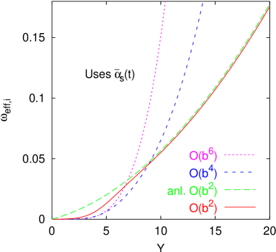
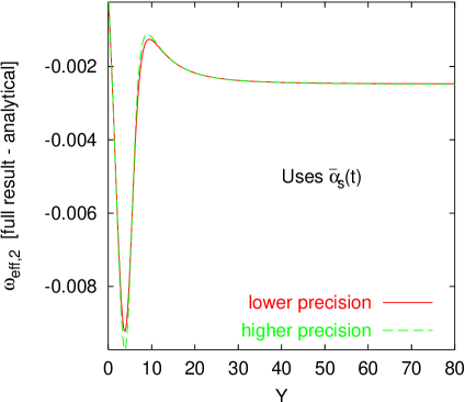
Figure 10: Left: terms in the $b$-expansion of $\omega_{\mathrm{eff}}(Y;t_{0},t_{0})$ up to order $b^{6}$, and additionally the asymptotic analytical prediction for the $b^{2}$ term ($b^{2}\alpha_{s}^{5}Y^{2}$ and $b^{2}\alpha_{s}^{4}Y$ contributions). Right: the difference between the full numerical result for the $b^{2}$ term and the asymptotic analytical result at lower and higher numerical precisions. In both cases ${\bar{\alpha}}_{s}(t_{0})=0.1$.

The $\mathcal{O}\left(b^{2}\right)$ term in the left-hand plot illustrates the characteristic $Y^{2}$ dependence expected from Eq. (44) (due to the derivative the contribution $b^{2}\alpha_{s}^{5}Y^{3}$ to $\ln G$ gives a contribution proportional to $Y^{2}$ in $\omega_{\mathrm{eff},2}$). It is compared to the sum of the analytically determined $b^{2}\alpha_{s}^{5}Y^{2}$ and $b^{2}\alpha_{s}^{4}Y$ terms and asymptotically one sees a good agreement. The right-hand plot shows the difference between the full numerical and partial analytical determination of $\omega_{\mathrm{eff},2}$ and one sees that it is consistent asymptotically with a constant term, which equals to $\delta\omega_{s}^{(2)}/b^{2}\simeq-0.002491$ from Eq. (46). The two curves in the right-hand plot have been determined with numerical evolutions of different accuracies so as to illustrate the numerical stability of the procedure. The differences visible at smaller $Y$ values are a consequence of sensitivity to the different approximations (widths) of the initial delta-function in $t$.

The left-hand plot also shows the $\omega_{\mathrm{eff},4}$ and $\omega_{\mathrm{eff},6}$ terms. While at low $Y$ they are suppressed, they grow much faster with $Y$ (as $Y^{4}$ and $Y^{6}$ respectively) and quickly dominate over the $\omega_{\mathrm{eff},2}$ term. Of course, they are suppressed in Eq. (71) by a power of $b$ also. But if we take $b=\mathcal{O}\left(1\right)$, then the $\zeta$ parameter in Eq. (42) is sizeable, and the importance of higher order terms increases with $Y$, meaning that the series (71) is slowly converging, because of nonanalyticity at $\zeta=\zeta_{c}$. This point will be discussed in more detail below and determines the perturbatively accessible range of $Y$ for BFKL predictions.

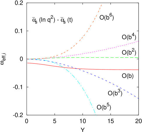
Figure 11: The difference between $\omega_{\mathrm{eff},i}(Y;t_{0},t_{0})$ for the case of a coupling that runs as ${\bar{\alpha}}_{s}(\ln q^{2})$ and one that runs as ${\bar{\alpha}}_{s}(t)$. Shown for ${\bar{\alpha}}_{s}(t_{0})=0.1$.

It is also of interest to examine what happens to the evolution when $\alpha_{s}$ is evaluated not at scale $t$ but at $\ln q^{2}$, which is favoured by the NLL corrections to the BFKL equation [3]. The differences in the $\omega_{\mathrm{eff},i}$ between these two options are shown in figure 11. This figure has been generated with a Gaussian ($\propto e^{-(t-t_{0})^{2}/2}$) initial condition as opposed to a delta-function, because with a delta-function, at small $Y$ one finds spuriously large contributions enhanced by logarithms of the ‘width’ of the delta-function.

With $\alpha_{s}(\ln q^{2})$ one loses the $b\leftrightarrow-b$ symmetry of the evolution and both odd and even powers of $b$ are present. At orders $b$ and $b^{2}$ the effect of changing from $\alpha_{s}(t)$ to $\alpha_{s}(\ln q^{2})$ is simply to modify $\omega_{\mathrm{eff}}$ by a constant — essentially the dynamics which led to the asymptotic $Y$-dependence in figure 10 is independent of what scale one chooses for $\alpha_{s}$. The constant shift is trivially $\Delta=-\omega_{s}^{0}\frac{b\omega_{s}^{0}}{2}$ at order $b$, and contains both scale changing and diffusion effects at order $b^{2}$. It is only at order $b^{3}$ and beyond that $Y$-dependence starts to appear, and one sees a form of mixing between the shift in $\omega_{\mathrm{eff}}$ which appears at relative order $b\omega_{s}^{0}$ due to the scale $\alpha_{s}(\ln q^{2})$ and the dynamical effects which arise for any choice of scale at relative order $(b{\bar{\alpha}}_{s}Y)^{2}$. This is reflected in the fact that the order $b^{3}$ and $b^{4}$ terms have a leading $Y^{2}$ dependence, while the $b^{5}$ and $b^{6}$ terms have a leading $Y^{4}$ dependence.

5.2 Pure perturbative predictions

One application of the $b$-expansion is that of extracting ‘purely perturbative’ numerical predictions.

One of the most common ways of obtaining BFKL predictions including running coupling is to solve Eq. (66) (or its analogues with various forms of higher-order correction) with a regularised running coupling, see for example [26, 27] . A measure of the perturbative uncertainty on the prediction can then be made by comparing different regularisations and seeing how they affect the Green’s function.

This is illustrated in Fig. 12a, which shows the Green’s function evaluated by direct numerical solution of Eq. (66) with two different regularisations of the coupling: in one the coupling is set to zero for $t<\bar{t}$ where ${\bar{\alpha}}_{s}(\bar{t})=0.5$, while in the other $\bar{t}$ is defined by ${\bar{\alpha}}_{s}(\bar{t})=0.25$. In this and other plots in this section, we use $\alpha_{s}(\ln q^{2})$ and the initial condition is a Gaussian rather than a delta-function so as to have sensible behaviour for $G$ at small $Y$.

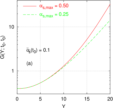
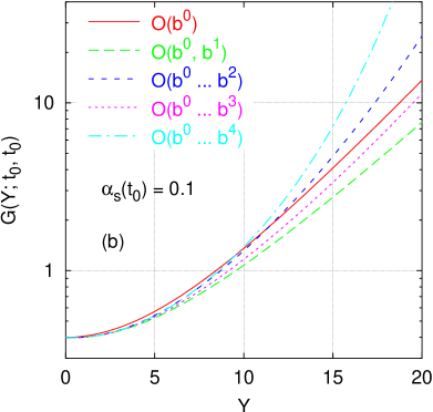
Figure 12: (a) the BFKL Green’s function evaluated with two regularisation of $\alpha_{s}$, a cutoff when ${\bar{\alpha}}_{s}=0.50$ and a cutoff when ${\bar{\alpha}}_{s}=0.25$; (b) the Green’s function evaluated by truncating the sum Eq. (69) at various orders.

At small and moderate $Y$ there is good agreement between the two curves, but beyond a certain point they no longer coincide, and one may deem this to be the limit of the perturbative prediction. However we could quite easily have chosen a different set of regularisations to compare to (e.g. with a coupling that freezes below $\bar{t}$) and one would have come to a different conclusion about the point where non-perturbative effects become important; it is difficult to make a strong case for one regularisation scheme as opposed to another.

A second point is that for small values of $\alpha_{s}(t_{0})$, in the numerical calculation the transition to the non-perturbative regime comes about by tunneling [12, 13], which places a limit on the maximum accessible rapidity, $Y_{\mathrm{max}}$, that scales as $1/\alpha_{s}(t_{0})$. However there are arguments that suggest that in the real world (as opposed to a numerical solution of a linear BFKL equation) effects such as unitarity [30, 31], or the fact that the Pomeron is soft, will eliminate or suppress tunneling. In such a situation the true non-perturbative limit on the maximum rapidity is believed to scale as $1/\alpha_{s}^{2}(t_{0})$ [18]. There is however a problem of how practically to calculate a Green’s function beyond the tunneling point.

The $b$-expansion offers a solution to both these problems. The question of how to determine the rapidity where perturbation theory breaks down reduces to that of establishing when the series expansion in $b$ stops converging. This is illustrated in Fig. 12b. One eliminates in this way the need for a subjective decision about a regularisation of the coupling. It is still necessary to decide where to truncate the series, but one has an analytical understanding of the properties of the series and the mathematical tools in such a case are well-established.

The problem of tunneling is also eliminated, because a truncated perturbative expansion in powers of $b$ will not reproduce a non-perturbative $e^{1/b\alpha_{s}}$ factor. The maximum perturbative rapidity in the $b$-expansion is therefore expected to behave precisely as discussed in [18], namely to scale as $1/\alpha_{s}^{2}(t_{0})$.

These ideas can be tested by considering a series of evolutions for different $\alpha_{s}(t_{0})$ values. In each case one establishes a maximum accessible rapidity, $Y_{\mathrm{max}}$, in two ways:

1. by examining when two non-perturbative regularisations lead to answers which differ by more than a certain threshold;

2. by examining when the difference between different truncations of the $b$-expansion differ by the same threshold.

In the first case we take the two regularisations used for Fig. 12a, while in the second case we take truncations at order $b^{3}$ and $b^{4}$. We define the threshold as being when $|\ln G_{a}/G_{b}|=0.2$, where $G_{a,b}$ are the Green’s function for the different regularisations or truncations.

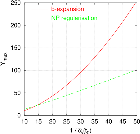
Figure 13: The maximum perturbatively accessible value of $Y$, as a function of $1/{\bar{\alpha}}_{s}(t_{0})$, determined by comparing different non-perturbative regularisations of $\alpha_{s}$, or different truncations of the $b$-expansion.

The results are shown in Fig. 13. There is a clear linear dependence on ${\bar{\alpha}}_{s}^{-1}(t_{0})$ for the case of the non-perturbative regularisation, a clear sign of tunneling being the relevant mechanism. In the $b$-expansion $Y_{\mathrm{max}}$ rises much more rapidly, in a manner quite compatible with a proportionality to ${\bar{\alpha}}_{s}^{-2}(t_{0})$. We note that the value of coefficient in front of ${\bar{\alpha}}_{s}^{-2}(t_{0})$, of the order of $0.1$, is in perfect agreement with the prediction based on the critical value $\zeta_{c}=0.26413$ found in Sec. 3.2, which yields $Y=\frac{\zeta_{c}}{b\chi_{m}}{\bar{\alpha}}_{s}^{-2}(t_{0})\simeq 0.104\;{\bar{\alpha}}_{s}^{-2}(t_{0})$.

Some comments are in order. For the case of nearly leading-log BFKL evolution that has been studied here, one could equally well have performed a normal expansion in powers of $\alpha_{s}$ for fixed $\alpha_{s}Y$ apart from the need of the Pomeron suppression. Indeed, it turns out that (for $t=t_{0}$) the $b^{i}\ell_{i}$ are functions only of $\alpha_{s}Y$ and $b\alpha_{s}$, and one can therefore rewrite the expansion for $\ln G$ as

$$\ln G\equiv\sum_{i=0}(b{\bar{\alpha}}_{s})^{i}\lambda_{i}(\alpha_{s}Y)$$ (72)

with $\lambda_{i}(\alpha_{s}Y)=\ell_{i}/\alpha_{s}^{i}=(\alpha_{s}Y)^{i+1}c_{i}+(\alpha_{s}Y)^{i}d_{i}+\dots,\hskip 8.5359pt(i\geq 1)$. From the point of view of Eq. (47) the highest $Y$ powers in $\lambda_{i}\sim(\alpha_{s}Y)^{i+1}$ correspond to the exponent function, the next-highest ones ($\sim(\alpha_{s}Y)^{i}$) to the normalisation, and lower ones to higher order fluctuations. Therefore, the $b$-expansion is needed to suppress the Pomeron, but is actually in one-to-one correspondence with an expansion in $\alpha_{s}$ at fixed $\alpha_{s}Y$.

For next-to-leading-logarithmic (and NⁿLL) evolution the situation is different. As is well known, the series convergence in $\alpha_{s}$ is extremely poor, because of several problems stemming essentially from large collinearly enhanced terms. To carry out an expansion in $\alpha_{s}$ for fixed $\alpha_{s}Y$ is therefore almost doomed to failure. The $b$-expansion will on the other hand be much more stable because at each order in $b$ one will effectively be able to resum collinearly-enhanced terms $\alpha_{s}^{n}(\alpha_{s}Y)^{m}$, in analogy with what is done in [20, 32]. The detailed behaviour is currently under investigation [19].

It is important keep in mind that after accounting for higher-order effects, the numerical values in figures such as Fig. 13 will be significantly altered, because on the one hand the diffusion coefficient is known to be very different at higher orders [3], and the tunneling behaviour is also expected to be numerically substantially modified. Nevertheless, we expect the qualitative features of that figure to persist.

Finally, one potential practical limitation of the $b$ expansion is the case when $t$ and $t_{0}$ are different, leading to the need for a collinear resummation. In such a case, as mentioned in Sec.3.2, in the regime where $t-t_{0}\ll t_{0}$, the coefficients of the $b$ expansion will be enhanced by powers of $(t-t_{0})$, and though the series may still be formally convergent, it is not clear whether it will be practical to include a sufficient number of terms for the convergence to be reached. To establish this point requires further investigation.

6 Conclusions

In this paper we have studied the properties of the gluon Green’s function in the case of the small-$x$ evolution equation with running coupling. In general the solution can be decomposed into perturbative — hard Pomeron and non-perturbative — Pomeron components. The hard Pomeron is then governed by the perturbatively calculable saddle point exponent $\omega_{s}(t)$ which is modified by the corrections due to running coupling effects. The non-perturbative part has instead a true singularity $\omega_{\mathrm{I\!P}}$ which is leading at large values of rapidity since $\omega_{\mathrm{I\!P}}>\omega_{s}(t)$. The Pomeron part is however suppressed at large values of $t$ by a tunneling factor which has a universal form of $\exp[-1/(b{\bar{\alpha}}_{s})g({\bar{\alpha}}_{s})]$. As a simple illustration, in the Airy diffusion model the Pomeron singularity is the lowest lying energy state of the potential in the Schroedinger-like problem. The perturbative part corresponds then to the continuum of states at $\mathrm{Re}\,\omega<0$. The decomposition into perturbative and non-perturbative parts is however non unique in the sense that some subleading bound states $\omega_{b}<\omega_{\mathrm{I\!P}}$ can be included in the perturbative part of the gluon Green’s function and are similar to a renormalon ambiguity.

Starting from this qualitative picture, we introduced the $b\rightarrow 0$, ${\bar{\alpha}}_{s}$ fixed limit in which the Pomeron is suppressed, in order to study the properties of the perturbative part $G_{pert}(Y;t,t_{0})$. By applying the $b$ expansion we obtained the saddle point exponent and the diffusion corrections. We showed that apart from the well known $\sim{\bar{\alpha}}_{s}^{5}Y^{3}$ corrections there are further subleading ones of type $\sim Y^{2}$ and $\sim Y$. The latter constitutes a second order $\omega_{s}$ shift, which adds up to dynamical corrections of the same order $b^{2}{\bar{\alpha}}_{s}^{2}Y$ coming from subleading corrections to the kernel. We have investigated in particular a scale change in the running coupling [19]. We found out that this perturbative expansion is controlled by the parameter $z=\frac{1}{2}(b{\bar{\alpha}}_{s})^{2}(\omega_{s}Y)^{2}\chi_{m}^{{}^{\prime\prime}}$ and is valid for $z\ll 1$. Outside this regime, when $z\gtrsim 1$, the perturbative solution starts to oscillate and the non-perturbative Pomeron takes over. Thus the genuine hard Pomeron part of the gluon Green’s function which is governed by $\omega_{s}(t)$ can be studied phenomenologically at large values of $t$ and moderate rapidities, in the limited regime where the non-perturbative part is strongly suppressed.

Additional NLL corrections are going to change the picture of diffusion and tunneling in a quantitative way. For example the so called kinematical constraint [33], incorporated in some resummations of subleading corrections [19] can be shown to increase the rapidity where tunneling occurs by about $t-t_{0}$; the proportionately larger effect of higher-order corrections at larger values of $\alpha_{s}$ will also delay the onset of tunneling, by reducing the non-perturbative Pomeron exponent. Both these effects can be expected to widen the window for phenomenological tests of the purely perturbative hard Pomeron. It should be also remarked that unitarity effects can in principle change significantly the phenomenon of tunneling. It was noticed in [30, 31] that in the case of the non-linear small $x$ evolution equation [34, 35], the generation of the saturation scale $Q_{s}(x)$ leads to the suppression of diffusion into the low scales $k<Q_{s}(x)$ and the distribution of the momenta is driven towards the perturbative regime. More detailed theoretical studies of these phenomena are thus needed.

7 Acknowledgments

This work was supported in part by the E.U. QCDNET contract FMRX-CT98-0194, MURST (Italy), the Alexander von Humboldt Stiftung and the Polish Committee for Scientific Research (KBN) grants no. 2P03B 05119, 2P03B 12019, 5P03B 14420.

Appendix A: Calculation of the fluctuations

The fluctuation matrix is obtained by taking the second derivatives with respect to $\gamma,\delta$ and $\omega$ of the exponent

$$E(\gamma,\delta,\omega)=\omega Y+(\gamma-1/2)t-(\gamma+\delta-1/2)t_{0}-\frac{1}{b\omega}X(\gamma)+\frac{1}{b\omega}X(\gamma+\delta)$$ (A.1)

in the double-$\gamma$ representation Eq. (38). It reads as follows:

$$\frac{1}{b\bar{\omega}}\left(\begin{array}[]{ccc}-2\chi^{\prime}(\bar{\gamma})&-\chi^{\prime}(\bar{\gamma})&0\\ &&\\ -\chi^{\prime}(\bar{\gamma})&-\chi^{\prime}(\bar{\gamma})&-bt\\ &&\\ 0&-bt&2bY\\ \end{array}\right)$$ (A.2)

where we have made use of the relations (40). The secular equation reads then

$$\left(\frac{2\chi^{\prime}(\bar{\gamma})}{b\bar{\omega}}+\lambda\right)\left(\frac{\chi^{\prime}(\bar{\gamma})}{b\bar{\omega}}+\lambda\right)\left(\frac{2Y}{\bar{\omega}}-\lambda\right)+$$ (A.3)

$$+ \left(\frac{2\chi^{\prime}(\bar{\gamma})}{b\bar{\omega}}+\lambda\right)\left(\frac{t}{\bar{\omega}}\right)^{2}+\left(\frac{\chi^{\prime}(\bar{\gamma})}{b\bar{\omega}}\right)^{2}\left(\lambda-\frac{2Y}{\bar{\omega}}\right)\;=\;0\;.$$

By looking at the separate terms in Eq. (A.3) it turns out that the sum and product of the eigenvalues have the following form ($\chi^{\prime}(\bar{\gamma})<0$)

$$\lambda_{1}+\lambda_{2}+\lambda_{3} = -\frac{3\chi^{\prime}(\bar{\gamma})}{b\bar{\omega}}+\frac{2Y}{\bar{\omega}}>0$$

$$\lambda_{1}\lambda_{2}\lambda_{3} = \frac{2\chi^{\prime}(\bar{\gamma})}{(b\bar{\omega})^{3}}[(bt)^{2}+bY\chi^{\prime}(\bar{\gamma})]<0\;,$$ (A.4)

which means that we have two positive eigenvalues and one negative - provided that

$$(b\,t)^{2}>-\chi^{\prime}(\bar{\gamma})\,b\,Y\;.$$ (A.5)

Since we have $bY=\zeta(bt)^{2}/\chi_{m}$, the condition (A.5) is equivalent to $\chi_{m}>-\zeta\chi^{\prime}(\bar{\gamma})$ and holds as long as $\zeta$ is a small parameter. Two positive eigenvalues correspond thus to fluctuations along the two imaginary axes and the negative eigenvalue to the fluctuation along the real axis in Eq. (38). After performing the integrations we obtain the following overall normalisation factor (using (A.4))

$$N(t,Y)\;=\;\frac{1}{(2\pi)^{2}}\frac{t_{0}}{\bar{\omega}}(2\pi)^{3/2}\frac{1}{\sqrt{-\lambda_{1}\lambda_{2}\lambda_{3}}}=\sqrt{\frac{b\bar{\omega}}{-4\pi\chi^{\prime}(\bar{\gamma})}}\frac{1}{\sqrt{1+\frac{\chi^{\prime}(\bar{\gamma})}{\chi_{m}}\zeta}}\;.$$ (A.6)

From (A.6) we can derive the subleading $\sim Y^{2}$ corrections. To this aim we expand, using (43), $\bar{\omega}$ and $\chi^{\prime}(\bar{\gamma})$ in $\zeta$ as follows

$$\bar{\omega} = \omega_{s}(t)(1+D\frac{\zeta^{2}}{4})+\dots$$

$$\chi^{\prime}(\bar{\gamma}=\frac{1}{2}-\bar{p}) = -\bar{p}\,\chi^{\prime\prime}(1/2)-\frac{1}{3!}\,\bar{p}^{3}\,\chi^{(4)}(1/2)=$$ (A.7)

$$= -\frac{\zeta}{2}(1+\frac{5}{12}D\zeta^{2})\left[\chi^{\prime\prime}(1/2)+\frac{1}{3!}\left(\frac{\zeta}{2}\right)^{2}\chi^{(4)}(1/2)\right]+\dots\;,$$

with $D=\chi_{m}^{{}^{\prime\prime}}/(2\chi_{m})$. Inserting (A.7) into (A.6) gives

$$N(t,Y) = \sqrt{\frac{b\omega_{s}}{2\pi\zeta\chi_{m}^{{}^{\prime\prime}}}}(1+\frac{1}{8}D\zeta^{2})(1-\frac{5}{24}D\zeta^{2})(1-\frac{1}{48}\frac{\chi_{m}^{(4)}}{\chi_{m}^{{}^{\prime\prime}}})(1+\frac{1}{2}D\zeta^{2})=$$ (A.8)

$$= \sqrt{\frac{1}{4\pi D\omega_{s}Y}}\left[1+D\zeta^{2}\left(\frac{5}{12}-\frac{1}{24}\frac{\chi_{m}^{(4)}\chi_{m}}{(\chi_{m}^{{}^{\prime\prime}})^{2}}\right)\right]\;.$$

Appendix B: Calculation of $Y^{2}$ and $Y$ terms in the Airy approximation

We show here how to obtain the quadratic $\sim Y^{2}$ and linear $\sim Y$ corrections to the saddle point exponent $\omega_{s}(t)$ in the case of the Airy diffusion model. We start from the exponent in the expression (61)

$$E\;=\;\omega_{s}(\tilde{t})|Y|\bigg{[}\frac{\xi(\xi-1)^{2}}{(-z)/3}+\bigg{(}\frac{\Delta t}{2\tilde{t}}\bigg{)}^{2}\frac{\xi}{(-z)}+\frac{1}{\xi}\bigg{]}\;,$$ (B.1)

and consider the expansion around the saddle point $\bar{\xi}$ defined by equation (62). We obtain

$$E=a_{0}+a_{1}\Delta\xi+\frac{1}{2}a_{2}(\Delta\xi)^{2}+\frac{1}{3!}a_{3}(\Delta\xi)^{3}+\dots\;,$$ (B.2)

where we defined

$$a_{n}\equiv{\partial^{n}E\over\partial\xi^{n}}\bigg{|}_{\xi=\bar{\xi}}\;,$$ (B.3)

and

$$\Delta\xi\equiv\xi-\bar{\xi}\;.$$ (B.4)

For simplicity we take ${\Delta t\over 2\tilde{t}}=0$. The saddle point condition $a_{1}=0$ results in equation (62) which at small values of $z$ has a solution (63) $\bar{\xi}=1-\frac{1}{6}z$ . The term $a_{0}$ instead provides the leading exponent $\omega_{s}$. The second derivative evaluated at $\bar{\xi}$ reads then

$$a_{2}\;=\;2\omega_{s}Y\left[{-3(3\bar{\xi}-2)\over z}+{1\over{\bar{\xi}}^{2}}\right]\;,$$ (B.5)

and the third one

$$a_{3}\;=\;-6\omega_{s}Y\left[{3\bar{\xi}\over z}+\frac{1}{\bar{\xi}^{4}}\right]\;.$$ (B.6)

We then expand the exponential in the following form

$$e^{\frac{1}{2}a_{2}(\Delta\xi)^{2}+\frac{1}{3!}a_{3}(\Delta\xi)^{3}}\simeq e^{\frac{1}{2}a_{2}(\Delta\xi)^{2}}\,[1+\frac{1}{3!}a_{3}(\Delta\xi)^{3}+\frac{1}{2}\left(\frac{a_{3}}{3!}\right)^{2}(\Delta\xi)^{6}\,]\;.$$ (B.7)

By integrating over $\Delta\xi$ the expression (B.7) we arrive at the following result

$$\sqrt{\frac{2\pi}{a_{2}}}\left(1+\frac{15}{16}\frac{2^{3}a_{3}^{2}}{(3!)^{2}a_{2}^{3}}\right)\;.$$ (B.8)

The first term in (B.8) i.e. the factor $\sqrt{2\pi/a_{2}}$ comes from the second order fluctuation and together with normalisation in (61) gives the following overall normalisation factor to $G_{pert}(Y;t,t_{0})$ and the $Y^{2}$ term

$$\frac{1}{2\pi\sqrt{D|z|/3}}\sqrt{\frac{\pi}{\omega_{s}Y\left[{-3\over z}(3\bar{\xi}-2)+{1\over{\bar{\xi}}^{2}}\right]}} \simeq \frac{1}{\sqrt{4\pi D\omega_{s}Y}}\frac{1}{\sqrt{1-\frac{5}{6}z}}\simeq$$ (B.9)

$$\simeq \frac{1}{\sqrt{4\pi D\omega_{s}Y}}(1+\frac{5}{12}z)\;,$$

which checks with the first term $\sim D\zeta^{2}$ in Eq. (A.8) (due to the Airy approximation we will not reproduce the second term with higher order derivatives).

The second term provides in turn the linear term in $Y$

$$\frac{15}{16}\frac{2^{3}a_{3}^{2}}{(3!)^{2}a_{2}^{3}}\simeq\frac{15}{16}\left(\frac{3\omega_{s}Y}{z}\right)^{2}\left(\frac{z}{3\omega_{s}Y}\right)^{3}=\frac{5}{16}\frac{z}{\omega_{s}Y}=\frac{5}{32}(b{\bar{\alpha}}_{s})^{2}{\bar{\alpha}}_{s}\chi_{m}^{\prime\prime}Y\;,$$ (B.10)

which is a second order shift to the saddle point value $\omega_{s}(t)$. The $(\Delta\xi)^{4}$ term in (B.7) can be safely neglected since it is of the subleading order $(b{\bar{\alpha}}_{s})^{4}$.

References

-
[1]
ZEUS Collab., M. Derrick et al., Phys. Lett. B316 (1993) 412;
ZEUS Collab., M. Derrick et al., Z. Phys. C 65, (1995) 379;
ZEUS Collab., M. Derrick et al., Z. Phys. C 72, (1996) 399;
ZEUS Collab., S. Chekanov et al., Eur. Phys. J. C21 (2001) 443;
H1 Collab., I. Abt et al., Nucl. Phys. B407, (1993) 515;
H1 Collab., S. Aid et al., Nucl. Phys. B 470, (1996) 3;
H1 Collab., C. Adloff et al., Nucl. Phys. B497, (1997) 3;
H1 Collab., C. Adloff et al., Eur. Phys. J. C 13, (2000) 609;
H1 Collab., C. Adloff et al., Eur. Phys. J. C 21 (2001) 33.
-
[2]
L. N. Lipatov, Sov. J. Nucl. Phys.
23 (1976) 338 ;
E. A. Kuraev, L. N. Lipatov, V. S. Fadin, Sov. Phys. JETP 45 (1977) 199;
I. I. Balitsky, L. N. Lipatov, Sov. J. Nucl. Phys. 28 (1978) 338. -
[3]
V. S. Fadin, M. I. Kotsky, R. Fiore,
Phys. Lett. B 359, (1995) 181;
V. S. Fadin, M. I. Kotsky, L. N. Lipatov, BUDKERINP-96-92, hep-ph/9704267;
V. S. Fadin, R. Fiore, A. Flachi, M. I. Kotsky, Phys. Lett. B 422, (1998) 287;
V. S. Fadin, L. N. Lipatov, Phys. Lett. B 429, (1998) 127;
G. Camici, M. Ciafaloni, Phys. Lett. B 386, (1996)341 ; Phys. Lett. B 412, (1997) 396 [Erratum-ibid. B 417, (1997)390 ]; Phys. Lett. B 430, (1998) 349. - [4] A.H. Mueller, H. Navelet, Nucl. Phys. B282 (1987) 727.
-
[5]
A.H. Mueller, Nucl. Phys. B (Proc. Suppl.)
18C,
(1990) 125;
A.H. Mueller, J. Phys. G 17, (1991) 1443;
J. Bartels, A. De Roeck, M. Loewe, Z. Phys. C 54, (1992) 635 ;
J. Kwieciński, A.D. Martin, P.J. Sutton, Phys. Rev. D 46, (1992) 921. - [6] for example see S.J. Brodsky, F. Hautmann, D.E. Soper, Phys. Rev. D56 (1997) 6957.
- [7] Y.V. Kovchegov, A.H. Mueller, Phys. Lett. B439 (1998) 428.
- [8] N. Armesto, J. Bartels, M.A. Braun, Phys. Lett. B442 (1998) 459.
- [9] E.M.Levin, Nucl. Phys. B453 (1995) 303; Nucl. Phys. B545 (1999) 481 .
- [10] J. Kwieciński, Z. Phys. C29 (1985) 561 .
- [11] J.C. Collins, J. Kwieciński Nucl. Phys. B316 (1989) 307.
- [12] M. Ciafaloni, D. Colferai, G. P. Salam, JHEP 9910 (1999) 017.
- [13] M. Ciafaloni, D. Colferai, G. P. Salam, A. M. Staśto, hep-ph/0204287.
- [14] A. Donnachie, P.V. Landshoff, Phys. Lett. B296 (1992) 227 .
- [15] A. Capella, A. Kaidalov, C. Merino, J. Tran Thanh Van, Phys. Lett. B337 (1994) 358; A. Capella, E.G. Ferreiro, C.A. Salgado, A.B. Kaidalov, Nucl. Phys. B593 (2001) 336.
- [16] R. S. Thorne, Phys. Rev. D64 (2001) 074005; Phys. Lett. B474 (2000) 372.
- [17] G. Altarelli, R. D. Ball, S. Forte, Nucl. Phys. B621 (2002) 359 .
- [18] M. Ciafaloni, A.H. Mueller, M. Taiuti, Nucl. Phys. B616 (2001) 349 .
- [19] M. Ciafaloni, D. Colferai, G. P. Salam, A. M. Staśto, in preparation.
-
[20]
M. Ciafaloni, D. Colferai, G. P. Salam, Phys. Rev. D60 (1999) 114036;
M. Ciafaloni, D. Colferai, Phys. Lett. B452 (1999) 372 . - [21] G. Altarelli, R. D. Ball, S. Forte, Nucl. Phys. B575 (2000) 313; Nucl. Phys. B599 (2001) 383.
- [22] S. J. Brodsky, V. S. Fadin, V. T. Kim, L. N. Lipatov, G. B. Pivovarov, JETP Lett. 70 (1999) 155.
- [23] C. R. Schmidt, Phys. Rev. D 60 (1999) 074003; MSUHEP-90416, hep-ph/9904368.
- [24] J. R. Forshaw, D. A. Ross, A. Sabio Vera, Phys. Lett. B455 (1999) 273.
- [25] V. S. Fadin, Nucl. Phys. A666 (2000) 155.
- [26] J. Kwiecinski, A. D. Martin and J. J. Outhwaite, Eur. Phys. J. C 9 (1999) 611.
- [27] B. Andersson, G. Gustafson and H. Kharraziha, Phys. Rev. D 57 (1998) 5543.
- [28] L. N. Lipatov, Sov. Phys. JETP 63 (1986) 904.
- [29] G. Camici , M. Ciafaloni, Phys. Lett. B395 (1997) 118 .
- [30] I. Balitsky, Phys. Lett. B518 (2001) 235 .
- [31] K. Golec-Biernat, L. Motyka, A. M. Staśto, Phys. Rev. D65 (2002) 074037.
- [32] G. P. Salam, JHEP 9807 (1998) 019.
-
[33]
M. Ciafaloni, Nucl. Phys. B296, (1988) 49;
B. Andersson, G. Gustafson, J. Samuelsson, Nucl. Phys. B467 (1996) 443;
J. Kwieciński, A. D. Martin, P. J. Sutton, Z. Phys. C 71 (1996) 585. - [34] I. I. Balitsky, Phys. Rev. Lett. 81 (1998) 2024; Phys. Rev. D60 (1999) 014020; JLAB-THY-00-44, hep-ph/0101042.
- [35] Yu. V. Kovchegov, Phys. Rev. D60 (1999) 034008; Phys. Rev. D61 (2000) 074018.