Classical gluodynamics in curved space–time
and the soft Pomeron

Abstract

QCD at the classical level possesses scale invariance which is broken by quantum effects. This “dimensional transmutation” phenomenon can be mathematically described by formulating classical gluodynamics in a curved, conformally flat, space–time with non–vanishing cosmological constant. We study QCD high–energy scattering in this theory. We find that the properties of the scattering amplitude at small momentum transfer are determined by the energy density of vacuum fluctuations. The approach gives rise to the power growth of the total hadron–hadron cross section with energy, i.e. the Pomeron. The intercept of the Pomeron and the multiplicity of produced particles are evaluated. We also speculate about a possible link between conformal anomaly and TeV scale quantum gravity.

1 Introduction

At the classical level, QCD is a scale invariant theory. Quantum fluctuations, however, give rise to scale anomaly [1] which is associated with dimensionful scale $\Lambda\approx 0.2$ GeV. The perturbative expansion is possible if the typical distance $Q^{-1}$ at which the interaction occurs is much smaller than $\Lambda^{-1}$, so the coupling is weak [2]: $\alpha_{s}(Q)\ll 1$. However, this does not mean that at short distances non-perturbative contributions can always be neglected. Indeed, the strength of the semi-classical vacuum fluctuations of the gluon field is inversely proportional to the coupling constant and thus can be large at short distances, when $\sim 1/\alpha_{s}(Q)\gg 1$. The goal of the present work is to derive an effective lagrangian for gluodynamics which makes it possible to systematically treat such contributions to the scattering amplitudes.

Gluodynamics is defined by the lagrangian

$$\mathcal{L}_{\mathrm{gluon}}=-\frac{1}{4}F^{a}_{\mu\nu}F^{a}_{\mu\nu}\quad.$$ (1)

If treated classically, this theory is invariant under the scale transformations $x\rightarrow\lambda x$. Transformation of scale is associated with the scale current $s_{\mu}$; its divergence is equal to the trace of the energy–momentum tensor:

$$\partial^{\mu}s_{\mu}=\theta_{\mu}^{\mu}(x).$$ (2)

Without quantum effects, $\theta_{\mu}^{\mu}(x)=0$, and the theory is scale invariant. Quantum effects break scale invariance [1]. However, the broken symmetry still manifests itself in the following set of low energy theorems for different Green functions involving operator $\theta_{\mu}^{\mu}(x)$ which can be proven by using renormalization group arguments [3]:

$$i^{n}\int dx_{1}\ldots dx_{n}\langle 0|T\{\theta_{\mu_{1}}^{\mu_{1}}(x_{1}),\ldots,\theta_{\mu_{n}}^{\mu_{n}}(x_{n})\}|0\rangle_{\mathrm{connected}}=\langle\theta_{\mu}^{\mu}(x)\rangle_{\mathrm{vac}}(-4)^{n}$$ (3)

In Ref. [4] it was shown that these low–energy theorems entirely determine the form of the effective low energy lagrangian for gluodynamics, which describes semi-classical vacuum fluctuations of gluon field at large distances. It is formulated in terms of an effective scalar dilaton field:

$$\mathcal{L}_{\mathrm{dilaton}}=\frac{|\epsilon_{\mathrm{v}}|}{m^{2}}\frac{1}{2}e^{\chi/2}(\partial_{\mu}\chi)^{2}+|\epsilon_{\mathrm{v}}|e^{\chi}(1-\chi)\quad,$$ (4)

where the real scalar field $\chi$ of mass $m$ represents the dilaton, and $-|\epsilon_{\mathrm{v}}|$ is the vacuum energy density.

The idea underlying the derivation can be formulated in the way which illustrates the analogy between gluodynamics and general relativity: QCD coupled to the conformally flat gravity is scale and conformally invariant in any number of dimensions, and thus such theory is anomaly–free. However, the vacuum energy density of flat–space gluodynamics $-|\epsilon_{\mathrm{v}}|$ (which plays a role of cosmological constant in general relativity) manifestly breaks scale and conformal symmetry of gluodynamics in conformally flat space-time. The low energy effective lagrangian (4) thus can be derived from the Einstein-Hilbert lagrangian for the described theory. Note that in the limit $|\epsilon_{\mathrm{v}}|\rightarrow 0$ lagrangian (4) is scale and conformally invariant, since another dimensionful parameter $m$ just sets the normalization of the dilaton field $\chi$. At small dilaton momenta $p\ll m$ the lagrangian (4) satisfies the low energy theorems (3). It is remarkable that the effective lagrangian involves only one scalar field. The reason is that the gravity is excited by the trace of energy momentum-tensor, so there is only one independent Einstein equation.

In the present work we are going to extend the range of validity of the effective lagrangian (4) to shorter distances by including the interactions of dilaton field with gluons. Generally, it can be obtained from the lagrangian of gluodynamics by integrating out soft gluon modes up to the scale $m$ which thus becomes the dimensionful scale of the theory. This implies that the scale $\Lambda$ and the dilaton mass $m$ are intimately connected. Actually, as we will show, it appears more convenient to construct the generalized effective lagrangian using Einstein equations once again. In the next section we employ this method to obtain the lagrangian (5). One can easily check that it is non-renormalizable. Therefore, we need to specify the additional dimensionful scale – the ultra-violet cutoff $M_{0}$. Obviously, $M_{0}$ is a function of $|\epsilon_{\mathrm{v}}|$ and $m$. It can be calculated using the requirement of vacuum stability, i.e.  all radiative corrections must cancel out to give correct value of vacuum energy density. Its numerical value turns out to be quite large, $M_{0}\sim 3$ GeV. This is in agreement with Ref. [3, 5, 6] where it has been argued that the typical scale of the vacuum gluon density due to semi-classical fluctuations can indeed be that large. In sec. 2 we discuss the effective lagrangian (5) in detail and calculate the scale $M_{0}$.

In sec. 3 we apply the effective lagrangian (5) to calculate a contribution of the non-perturbative semi-classical fluctuations of the QCD vacuum to the pomeron intercept. Experimental data on different reactions at high energies and small momentum transfer support existence of the pole in the scattering amplitude responsible for high energy behavior of the total cross sections [7]. This leads to the power-like behavior of the total cross section $\sigma_{\mathrm{tot}}=\varsigma\,s^{\alpha_{P}-1}$, where $\varsigma$ depends upon particular reaction and $\alpha_{P}$ is the universal parameter called the intercept. After decades of hard work, understanding the nature of the object exchanged in $t$-channel (pomeron) is still a challenging problem. It turned out that the perturbative QCD is far from giving a clear answer even if the scales inherent to colliding particles are hard. Partly, this is due to diffusion of the transverse momenta in the partonic cascade towards the non-perturbative scales. This implies that the main contribution to the pomeron stems, perhaps, from the non-perturbative sector of QCD. Assuming that some non-perturbative fluctuations of vacuum dominate the scattering amplitude at high energies one has to explain the power-like behavior of the total cross section $\sigma_{\mathrm{tot}}\sim s^{\alpha_{P}-1}$ and to obtain the correct numerical value of $\alpha_{P}$. A few authors have reported on this problem. Contribution of instantons to the scattering amplitude at high energies was investigated in Ref. [8, 9]. In Ref. [10] it has been argued that fluctuations of strings in the framework of AdS/CFT theory can yield the desired result. In Refs. [11, 12] the spectrum of glueballs in QCD was discussed as well as its relation to the structure of the pomeron. Possible contributions of extra compact dimensions was discussed in Ref. [13, 14]. A more phenomenological approach has been developed in framework of the BFKL gluon emission with additional assumption for such an emission in the non-perturbative QCD domain [15]. In Ref. [16] two of us have used the fact that the non-perturbative QCD vacuum is dominated by the semi-classical fluctuations of the gluon field which is inversely proportional to the coupling $F\sim 1/g$. The importance of such fluctuations can be understood in the following way. Consider a gluon ladder in each rung of which two gluons in a singlet state are produced in $s$-channel. Each rung gives contribution of the order $g^{2}F^{2}\sim\mathcal{O}{(1)}$ since the two-gluon singlet state gives contribution proportional to the trace of energy-momentum tensor. Such ladder diagrams can be summed up yielding a reasonable value of the pomeron intercept. In the present paper we suggest a method for systematic calculation of processes involving such non-perturbative modes of gluodynamics. In particular, we will calculate the total cross section at high energies, reproduce its power-like behavior and numerical value of the intercept. We also calculate the final state multiplicity in this approach.

We conclude the paper by presenting some speculative ideas on the possible link between QCD and gravity. Recall that the effective lagrangian (5) can be derived from the General Relativity. Thus the gravitational constant can be expressed in terms of the dilaton mass and the vacuum energy density, Eq. (11). Its numerical value $G=0.2\,\mathrm{GeV}^{-2}$, of course, has nothing to do with the Planck gravitational constant. Nevertheless, it may be possible to interpret this result as a signature of the strong gravitational interactions at scale much lower than the Planck one. If we accept this interpretation, then it turns out that the gravitational effects are essential already at the GeV scale, in order to be responsible for the QCD vacuum structure. Several authors have suggested mechanisms by which gravitational interactions can become strong at scales much larger than the Planck one [17]. Recently it has been suggested that quantum gravity can become strong at the TeV scale [18]. In sec. 4 we briefly discuss those ideas.

2 Dilaton effective lagrangian

The dilaton effective lagrangian in gluodynamics describing the propagation and interactions of gluon and dilaton fields can be constructed as a generalization of Eqs. (4),(1). It reads

$$\mathcal{L}=\frac{|\epsilon_{\mathrm{v}}|}{m^{2}}\frac{1}{2}e^{\chi/2}(\partial_{\mu}\chi)^{2}+|\epsilon_{\mathrm{v}}|e^{\chi}(1-\chi)-e^{\chi}(1-\chi)\frac{1}{4}F^{a}_{\mu\nu}F^{a\mu\nu}\quad.$$ (5)

Eq. (5) can be obtained utilizing Legendre transformation of the lagrangian describing coupling of gluodynamics to gravity

$$\mathcal{L}^{\prime}=\left(\frac{1}{8\pi G}R-\frac{1}{4}F^{a}_{\mu\nu}F^{a\mu\nu}+|\epsilon_{\mathrm{v}}|\right)\sqrt{-\det g_{\mu\nu}}\quad.$$ (6)

The first term in (6) corresponds to the gravitational lagrangian $\mathcal{L}_{G}$. It is expressed through the Ricci scalar $R$ which can be easily calculated for the conformally trivial metric $g_{\mu\nu}=\eta_{\mu\nu}e^{h(x)}$

$$\mathcal{L}_{G}=\frac{1}{8\pi G}R\sqrt{-\det g_{\mu\nu}}=\frac{1}{8\pi G}3e^{h}\left(\partial^{2}_{\mu}h+\frac{1}{2}(\partial_{\mu}h)^{2}\right)=-\frac{1}{8\pi G}\frac{3}{2}e^{h}(\partial_{\mu}h)^{2}\quad,$$ (7)

where we have used integration by parts to derive the last equation and $\eta_{\mu\nu}=\mathrm{diag}\!\{1,-1,-1,-1\}$. In (7) $G$ is the gravitational constant. The gravitational field $h$ couples to the gluodynamics by means of the second term

$$-\frac{1}{4}F^{a}_{\mu\nu}F^{a\mu\nu}e^{2h}\quad.$$

These two terms are invariant under scale and conformal transformations in a space-time of arbitrary dimension. However, the scale symmetry in QCD is broken down by non-vanishing gluon condensate $\langle F^{a}_{\mu\nu}F^{a}_{\mu\nu}\rangle$$>0$. This leads to the scale anomaly which manifests itself as an anomaly of the QCD energy-momentum tensor ($\theta^{\mu\nu}$) trace

$$\theta^{\mu}_{\mu}=\frac{\beta(g)}{2g}F^{a}_{\mu\nu}F^{a\mu\nu}\quad,$$ (8)

where the $\beta$-function in the leading order in the strong coupling $g$ reads

$$\beta(g)=-\frac{11\,g^{3}}{(4\pi)^{2}}\quad.$$ (9)

Its vacuum expectation value is

$$\langle\theta^{\mu}_{\mu}\rangle=-4|\epsilon_{\mathrm{v}}|\quad.$$ (10)

In order for the energy-momentum tensor, calculated from the lagrangian (6) to satisfy (10), the third term in (6) which explicitly breaks the scale invariance has been introduced. This term can also be thought of as the cosmological constant. In the absense of the gravitational part (7) of the lagrangian (5) the condition (10) is satisfied trivially at the tree level. Performing the Legendre transformation of (6) one arrives at (5) [4]. The mass of the dilaton can be expressed through the vacuum energy density and the gravitational constant as follows

$$m^{2}=\frac{64\pi}{3}\,|\epsilon_{\mathrm{v}}|\,G\quad.$$ (11)

Now we require the energy momentum tensor calculated from the lagrangian (5) to satisfy the vacuum normalization condition (10). This means cancelation of the dilaton and gluon contributions to the vacuum energy density. We can formulate (10) in terms of the vacuum expectation values. To this end let us calculate the trace of the energy-momentum tensor

$$\theta_{\mu}^{\mu}=\eta^{\mu\nu}\left(2\frac{\partial\mathcal{L}}{\partial\eta^{\mu\nu}}-\eta^{\mu\nu}\mathcal{L}\right)+\frac{8|\epsilon_{\mathrm{v}}|}{m^{2}}\partial_{\mu}^{2}\,e^{\chi/2}\quad,$$ (12)

where the last term in the right hand side is the total derivative [4]. Equation of motion for the dilaton field is

$$\frac{|\epsilon_{\mathrm{v}}|}{m^{2}}\,\partial_{\mu}\left(e^{\chi/2}\,\partial_{\mu}\chi\right)-\frac{|\epsilon_{\mathrm{v}}|}{4m^{2}}\,e^{\chi/2}\left(\partial_{\mu}\chi\right)^{2}+\chi\,e^{\chi}\,|\epsilon_{\mathrm{v}}|-\chi\,e^{\chi}\,\frac{1}{4}\,F_{\mu\nu}^{a}F^{a\mu\nu}=0\quad.$$ (13)

Using (13) in (12) we arrive at

$$\theta_{\mu}^{\mu}=-4\,|\epsilon_{\mathrm{v}}|\,e^{\chi}+\chi\,e^{\chi}\,F_{\mu\nu}^{a}F^{a\mu\nu}\quad.$$ (14)

Hence, (10) is equivalent to the following relation

$$\langle\;\chi\,e^{\chi}\,F_{\mu\nu}^{a}F^{a\mu\nu}\;\rangle=4\,|\epsilon_{\mathrm{v}}|\;\langle\,e^{\chi}-1\;\rangle\quad.$$ (15)

It is clear from equations (14) and (13) that in the limit $|\epsilon_{\mathrm{v}}|\rightarrow 0$ the classical equation $\theta_{\mu}^{\mu}=0$ is recovered. However, quantum corrections can give non–vanishing contributions to $\langle\theta_{\mu}^{\mu}\rangle$ in the same limit by introducing dimensonal cutoff. Eq. (15) assures that this does not happen in our theory.

Now, we proceed to the derivation of Feynman rules. In addition to usual Fyenman diagrams of gluodynamics there are those corresponding to the dilaton propagator, dilaton self-interactions and dilaton-gluon interactions. In this work we are interested only in contributions of the order of $g^{0}$. They are shown in Fig. 1. Other vertices, which contain three and four gluons coupled to the dilaton are supressed by factors $g^{1}$ and $g^{2}$ respectively. In our approach the strong coupling constant is necessarily small since all gluon modes which enter the lagrangian (5) are hard by construction. All soft modes, which carry momenta $p<m$, have been integrated out. The dilaton Feynman propagator can be read from (5):

$$D_{d}(p)=\frac{m^{2}}{|\epsilon_{\mathrm{v}}|}\ \frac{i}{p^{2}-m^{2}-i\varepsilon}\quad.$$ (16)

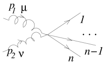
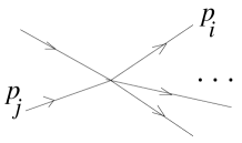
$(n-1)\,(p_{1}^{\nu}p_{2}^{\mu}-(p_{1}\cdot p_{2})\eta^{\mu\nu})\delta^{ab}$		$-|\epsilon_{\mathrm{v}}|\left\{(n-1)+\frac{2}{n(n-1)}\sum_{i>j}\frac{1}{2^{n}m^{2}}(p_{i}\cdot p_{j})\right\}$
$n=2,3,\ldots$		$n=3,4,\ldots$
(a)		(b)

Figure 1: Feynman diagrams of order $g^{0}$ and given number of dilatons $n$; (a) gluon-dilaton interaction, (b) dilaton self interaction.

To completely specify our effective theory we still have to calculate the ultra-violet cutoff $M_{0}$. Contributions to the vacuum energy density involve loops and therefore they are divergent in the ultra-violet regime of the theory. Let us introduce the cut-off $M_{0}$ which controls divergences of vacuum excitations contributing to the vacuum expectation value of the trace of the energy-momentum tensor. The same parameter controls divergences in the dilaton phase space. Our requirement that the normalization (10), or equivalently (15), holds means that we impose a restriction on the possible values of $M_{0}$. Consider a contribution stemming from pure dilaton vacuum fluctuations, Fig. 2(a).

(a)	(b)

Figure 2: Some vacuum excitations contributing to the energy-momentum tensor trace. (a) Dilaton self-interactions; first diagram is proportional to $\langle\chi^{2}\rangle$, (b) dilaton-gluon interactions.

In the next section we will argue that for the processes we are interested in here the phase space is available for the emission of only two dilatons. In this two-dilaton approximation

$$\langle\theta_{\mu}^{\mu}\rangle_{\mathrm{vac}}=-4|\epsilon_{\mathrm{v}}|\langle e^{\chi}\rangle_{\mathrm{vac}}\approx-4|\epsilon_{\mathrm{v}}|\left(1+\frac{1}{2}\langle\chi^{2}\rangle_{\mathrm{vac}}\right)\quad.$$ (17)

Hence, the contribution to the vacuum energy-density is

$$-2|\epsilon_{\mathrm{v}}|\langle\chi^{2}\rangle_{\mathrm{vac}}=-2|\epsilon_{\mathrm{v}}|\frac{1}{\pi}\int_{0}^{M_{0}^{2}}\frac{dM^{2}}{M^{2}}\,\frac{m^{2}}{|\epsilon_{\mathrm{v}}|}\int\frac{d^{3}k}{(2\pi)^{3}2\omega}=-\frac{1}{4\pi^{3}}m^{2}M_{0}^{2}\quad.$$ (18)

Another contribution of the same order in the strong coupling, $\mathcal{O}{(g^{0})}$, comes from the first diagram shown in Fig. 2(b). We have

$$(N_{c}^{2}-1)\,\frac{1}{\pi}\int_{0}^{M_{0}^{2}}\frac{dM^{2}}{M^{2}}\;\frac{1}{2!}\int\,\frac{d^{3}q_{1}}{(2\pi)^{3}2\omega_{1}}\int\,\frac{d^{3}q_{2}}{(2\pi)^{3}2\omega_{2}}\Gamma_{2}\left(q_{1}^{\nu}q_{2}^{\mu}-(q_{1}\cdot q_{2})\eta^{\mu\nu}\right)^{2}\theta(M-\omega_{1}-\omega_{2})$$

$$=\;\frac{M_{0}^{8}}{280\cdot 48\,(2\pi)^{6}}\,(N_{c}^{2}-1)\,\left(\frac{m^{2}}{|\epsilon_{\mathrm{v}}|}\right)^{2}\quad,$$ (19)

where $\Gamma_{2}$ is a two-dilaton phase-space factor, see (28). Contributions (18) and (19) cancel out when

$$M_{0}^{2}=8\pi\,2^{2/3}\,105^{1/3}\,(N_{c}^{2}-1)^{-1/3}\,\left(\frac{|\epsilon_{\mathrm{v}}|}{m}\right)^{2/3}\quad.$$ (20)

The pure gluon vacuum diagrams are proportional to the strong coupling constant $\alpha_{s}$ as can be easily seen from (8) and (9). Inasmuch as the strong coupling constant is small, those contributions to the vacuum energy density can be neglected.

3 Derivation of the soft pomeron

The leading contribution to the total cross section at high energies stems from the ladder diagrams [19]. Such a diagram is shown in Fig. 3. Note that the energy dependence of the Born amplitude is determined by the spin of particles exchanged in $t$-channel. Thus the leading contribution at high energies comes from exchange of vector particles – gluons [20, 21]. These gluons prefer to form ladders, since each rung gets enhanced by large logarithm of energy $\ln s\gg 1$. By virtue of the optical theorem, the total cross section $\sigma_{tot}$ can be calculated as a sum of all such diagrams

$$\sigma_{tot}=\sum_{r\geq 0}\sum_{n\geq 2}\sigma_{r}^{n}=\frac{2}{s}\sum_{r\geq 0}\sum_{n\geq 2}\mathrm{Im}\,\mathcal{M}_{\mathrm{el}}(t=0)_{r}^{n}\quad,$$ (21)

i.e.  we sum over all possible numbers $n\geq 2$ of dilatons produced in $s$-channel in each rung for a given number $r$ of rungs and then sum over all $r$.

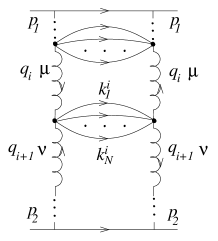
Figure 3: One of the ladder diagrams contributing to eq. (21).

The most convenient way to calculate the amplitudes associated with ladder diagrams is to employ the Weizsäcker-Williams approximation. This means replacing almost longitudinally polarized Coulomb gluons exchanged in $t$-channel by transversely polarized (real) ones. In this approximation the gluon propagator reads [21]:

$$D_{g}(q^{2})\,\approx\,\frac{2}{s}\frac{q_{\bot}^{\mu}q_{\bot}^{\nu}}{\alpha_{q}\beta_{q}q_{\bot}^{2}}\quad,$$ (22)

where $\alpha_{q}$ and $\beta_{q}$ are Sudakov variables defined by

$$q=\alpha_{q}\,p_{1}+\beta_{q}\,p_{2}+q_{\bot}\quad.$$ (23)

Weizsäcker-Williams approximation is valid as long as the following conditions hold

$$1\gg\alpha_{q_{1}}\gg\ldots\gg\alpha_{q_{i}}\gg\ldots\gg\alpha_{q_{r+1}}\quad,$$ (24)

$$1\gg\beta_{q_{r+1}}\gg\ldots\gg\beta_{q_{i}}\gg\ldots\gg\beta_{q_{1}}\quad,$$ (25)

$$|q_{i\bot}^{2}|\ll s\quad.$$ (26)

In the Born approximation (two gluon exchange) there are no produced dilatons. Contribution of a one-rung diagram to the total cross section reads

$$\sigma_{r=1}^{n}=\frac{2}{s}\int\frac{d^{4}q_{1}}{(2\pi)^{4}}\int\frac{d^{4}q_{2}}{(2\pi)^{4}}\left|\frac{2g^{2}(q_{1}\cdot q_{2})_{\bot}\mathrm{Tr\,}(t^{a}t^{b})}{\beta_{q_{1}}\alpha_{q_{2}}s}\right|^{2}\frac{1}{4N_{c}^{2}}(2\pi)^{2}\delta((p_{1}-q_{1})^{2})\delta((p_{2}+q_{2})^{2})\Gamma_{n}(M)\quad,$$ (27)

where $\Gamma_{n}(M)$ represents contribution of $n$ dilatons to the phase space and $M^{2}=(q_{1}-q_{2})^{2}$ is the four-momentum squared available for production in the dilaton vertex. The phase space $\Gamma(M)$ has been evaluated in Ref. [8]:

$$\Gamma_{n}(M)=\frac{1}{n!}\left(\frac{m^{2}}{|\epsilon_{\mathrm{v}}|}\right)^{n}\,(n-1)^{2}\,(2\pi)^{4}\,\delta^{4}\left(\sum_{i=1}^{n}k_{i}-k\right)\prod_{i=1}^{n}\frac{d^{3}k_{i}}{(2\pi)^{3}2\omega_{i}}$$

$$=\left(\frac{m^{2}}{|\epsilon_{\mathrm{v}}|}\right)^{n}(2\pi)^{4-3n}\,(n-1)^{2}\,\frac{(\pi/2)^{n-1}(M^{2})^{n-2}}{n!(n-1)!(n-2)!}\quad,$$ (28)

where $(n-1)^{2}$ comes from the vertex shown in Fig. 1(a). Using (27) and (28) we derive the contribution of one-ladder diagram

$$\sum_{n\geq 2}\sigma_{r=1}^{n}=\sigma_{B}\frac{\ln s}{(2\pi)^{6}}\pi^{2}M_{0}^{2}\int_{0}^{M_{0}^{2}}\,dM^{2}\,\sum_{n=2}^{\infty}\Gamma_{n}(M)=\sigma_{B}\Delta_{P}\ln s\quad,$$ (29)

where $\sigma_{B}\sim\alpha_{s}$ is a Born amplitude,

$$\Delta_{P}=\frac{a^{2}}{4\pi}\;_{0}F_{2}\left(-;1,3;a\right)\quad,$$ (30)

${}_{0}F_{2}$ is a generalized hypergeometric function, and the relevant parameter of our theory for high energy scattering is

$$a=\frac{m^{2}M_{0}^{2}}{16\pi^{2}\,|\epsilon_{\mathrm{v}}|}\quad.$$ (31)

Expansion of function ${}_{0}F_{2}$ in powers of parameter $a$

$$_{0}F_{2}\left(-;1,3;a\right)=1+\frac{a}{3}+\frac{a^{2}}{48}+\frac{a^{3}}{2160}+\mathcal{O}{(a^{4})}$$ (32)

is equivalent to expansion in the number of emitted dilatons. We will argue below that the series (32) are rapidly convergent and actually, there is not enough phase space for emission of large number $n$ of dilatons since $\Gamma_{n}(M)$ is a rapidly decreasing function of $n$. Thus, we can safely neglect emission of more than two dilatons.

Now, as we know the contribution of one-rung diagram, calculation of the total cross section is straightforward. Indeed, the contributions of different rungs factorize out, leading to the Regge-like behavior of the total cross section (21)

$$\sigma_{tot}=\sigma_{B}\sum_{r=0}^{\infty}\frac{1}{r!}\ln^{r}s\,\Delta_{P}^{r}=\sigma_{B}\,s^{\Delta_{P}}\quad.$$ (33)

Corrections to the pomeron intercept coming from perturbative QCD are proportional to the strong coupling constant $g^{2}$ and neglected in this approach. Loop corrections to the dilaton propagator give small contributions of the order of

$$\Delta D_{d}\,\sim\,\frac{am^{2}}{M_{0}^{2}}\ll 1\quad.$$

Finally, upon substitution of (31) and (20) into (30) we obtain the following result for the soft pomeron intercept

$$\alpha_{P}=1+\Delta_{P}=1+\frac{(105/2)^{2/3}}{4\pi^{3}}\,(N_{c}^{2}-1)^{-2/3}\,\left(\frac{m^{4}}{|\epsilon_{\mathrm{v}}|}\right)^{2/3}\quad.$$ (34)

To estimate $|\epsilon_{\mathrm{v}}|$ in pure gluodynamics we use the fact that it is related to the vacuum energy density in QCD $|\epsilon_{\mathrm{v}}|_{\mathrm{QCD}}$ by

$$|\epsilon_{\mathrm{v}}|\simeq\frac{11}{9}\,3\,|\epsilon_{\mathrm{v}}|_{\mathrm{QCD}}\quad.$$ (35)

Indeed, as was argued in Ref. [3],

$$\langle\alpha_{s}F_{\mu\nu}^{a}F^{a\mu\nu}\rangle_{\mathrm{glue}}\,\approx\,3\,\langle\alpha_{s}F_{\mu\nu}^{a}F^{a\mu\nu}\rangle_{\mathrm{QCD}}\quad.$$ (36)

Also the beta function (9) in QCD scales with number of col-ours and flavors as $\beta_{\mathrm{QCD}}\propto(11N_{c}-2N_{f})/3$ whereas in pure gluodynamics $\beta_{\mathrm{glue}}\propto 11N_{c}/3$. Since by (8) $|\epsilon_{\mathrm{v}}|\propto\beta$ the vacuum energy density in pure gluodynamics gets enhanced by the factor $11/9$. Together with (36) this yields (35). Sum rules analysis of [3] makes it possible to estimate the QCD vacuum energy density $|\epsilon_{\mathrm{v}}|_{\mathrm{QCD}}=(0.24\,\mathrm{GeV})^{4}$. Owing to (35) we obtain the following estimate:

$$|\epsilon_{\mathrm{v}}|=0.012\,\mathrm{GeV}^{4}\quad.$$ (37)

Another parameter of our effective theory is the dilaton mass. Note, that due to the isospin conservation each dilaton can produce only even number of pions in the final state. Let us assume that in full QCD with light quarks the dilaton mixes with the broad physical scalar $\sigma$–resonance [1] at

$$m=0.4\div 0.5\,\mathrm{GeV}\quad.$$ (38)

Note that the spectral density of the dilaton excitations can be spread over several scalar resonances of different mass (see, e.g., [23]). However, for our purposes it suffices to keep only the lightest resonance, which gives the dominant contribution to the intercept because of the phase space constraints.

Let us now proceed to the numerical estimates. In view of (37) and (38) Eq. (20) implies that $M_{0}=3.0\div 2.8\,\mathrm{GeV}$. Substituting these numbers to (34) we obtain for the pomeron intercept $\alpha_{P}=1.047\div 1.085$ which is in reasonable agreement with the phenomenology of high energy scattering [22]. Using these numbers in (32), we see that the emission of three and more dilatons contributes $1-{{}_{0}F_{2}}\left(-;1,3;0\right)/_{0}F_{2}\left(-;1,3;a\right)$=$21\div 27\%$ to the final result; this can be used as an estimate of the accuracy of our two-dilaton approximation.

We can calculate the inclusive spectrum of dilaton production by observing that Eq. (28) is nothing but the number distribution of the dilatons produced per unit of rapidity. Indeed, each rung of the ladder diagram corresponds to one unit in rapidity (multiplied by $\Delta_{P}$) in the leading logarithmic approximation. Define the probability $P_{n}(a)$ to find $n$ dilatons in the final state

$$P_{n}(a)=\frac{\int_{0}^{M_{0}^{2}}dM^{2}\;\Gamma_{n}(M)}{\sum_{n=2}^{\infty}\int_{0}^{M_{0}^{2}}dM^{2}\;\Gamma_{n}(M)}\quad.$$ (39)

Then the average number of dilatons produced per unit of rapidity is given by

$$\langle\frac{dN_{\chi}}{d(\Delta_{P}\,y)}\rangle=\sum_{n=2}^{\infty}n\,P_{n}(a)=\frac{2\;_{0}F_{2}\left(-;1,2;a\right)}{{}_{0}F_{2}\left(-;1,3;a\right)}\quad.$$ (40)

From (31) we get an estimate of the dilaton phase space parameter $a=0.768\div 1.033$. Substituting this value into (40) one arrives at $\langle dN_{\chi}/dy\rangle=0.1\div 0.2$. Since we have identified the dilaton with the physical $\sigma$-resonance, we have to assume that it decays mostly in two pions. Charged pions give approximately 2/3 of the total number of pions. Therefore, the average multiplicity of charged pions per unit of rapidity is estimated as

$$\langle\frac{dN_{\pi}^{\mathrm{ch}}}{dy}\rangle\,=\,\frac{2}{3}\,2\,\langle\frac{dN_{\chi}}{dy}\rangle\,=\,0.14\div 0.26\quad.$$ (41)

This agrees with the result obtained in[16]: the soft pomeron is responsible for less then 10% of the observed multiplicity. In Fig. 4 we show the number distribution (39) of produced charged pions.

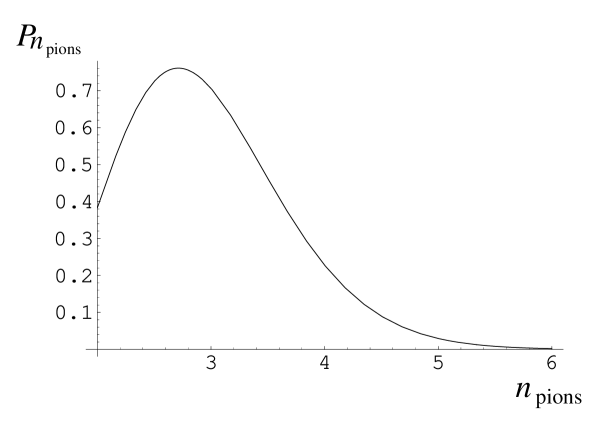
Figure 4: Number distribution of charged pions produced by dilaton mechanism for $a=0.9$ at hadron-hadron collisions.

4 Summary and discussion

Summarizing, we have started with the derivation of the QCD effective lagrangian (5) which incorporates scale anomaly[1, 4] and represents propagation and interaction of gluons and dilatons. The dilaton field saturating the sum rules (3) describes the QCD vacuum structure. The pure dilaton part of lagrangian (5) (first and second terms) is a low energy effective gluodynamics obtained by integrating out low energy modes with momenta $q$ such that $q\leq m\approx 0.4\div 0.5$ GeV. The third term of (5) represents pure gluodynamics and the interaction of gluon field with the dilaton one. It is important as far as momentum transfer does not exceed $M_{0}$. It has been already pointed out in Ref. [3, 5, 16] that the scale $M_{0}$, determined by the semi-classical fluctuations of the gluon fields in vacuum is quite large, $M_{0}\gg\Lambda$.

Normalizing the vacuum energy density by (10) we obtained an expression (20) for the ultra-violet cutoff $M_{0}$ of the theory in terms of vacuum energy density $|\epsilon_{\mathrm{v}}|$ and the dilaton mass $m$. Divergent integrals that we have encountered in Eqs. (18),(19),(29) should not surprise the reader since the dilaton acts as the gravitational field. Indeed, quantum gravity is a non-renormalizable theory since the coupling of gravity to matter fields $G$ has canonical dimension (mass)^-2. In technical terms, each emitted dilaton contributes a factor of $m^{2}/|\epsilon_{\mathrm{v}}|$ coming from the normalization of the dilaton propagator which must be compensated for by $M_{0}^{2}$ to maintain the scattering amplitude dimensionless.

In the framework of this effective theory we addressed the problem of soft pomeron. We calculated the high energy scattering amplitude in the leading logarithmic approximation by summing the ladder diagrams, see Fig. 3. Generally, any number of dilatons can be emitted in the $t$-channel in each ladder rung, but actually most of the phase space is occupied by only two of them. Owing to the isospin conservation the dilaton in the final state decays into an even number of pions. By identifying the dilaton with the physical $\sigma$ resonance, we conclude that it should decay mostly in two pions. We estimate the pomeron intercept $\alpha_{P}=1.047\div 1.085$. This value agrees well with the analysis of the data on high energy scattering [22].

We also estimate the final state multiplicity per unit of rapidity $\langle\frac{dN_{\chi}}{dy}\rangle\simeq 0.2$. The low particle multiplicity resulting from the soft pomeron exchange has been noted already in [16]. It implies that the bulk of particles is produced by another mechanism. Such a mechanism must involve multiple production of particles per unit of rapidity and perhaps closely related to high parton density regime of QCD [21, 24].

The reader familiar with the previous work of two of us, Ref. [16], might be confused by the fact that there the opposite to (34) dependence of $\Delta$ on the vacuum energy density $|\epsilon_{\mathrm{v}}|$ and the scalar particle (glueball) mass $m_{R}$ has been found. The reason is simple: a glueball mediates a short-range strong interaction, so the cross section for its production is proportional to $m_{R}^{-4}$. On the other hand, gravitation is a long-range interaction, the strength of which is proportional to masses of interacting particles (dilatons). In other words, the effective lagrangian (5) is constructed to obey scale invariance on the classical level. This requirement translates into the absence of the coupling of the dilaton to two gluons, because a term linear in the dilaton field $\chi$ in (5) would induce a non-zero vacuum expectation value $\langle\chi\rangle$ which would violate the scale invariance already on the classical level. (Even though the field $\chi$ is dimensionless, its couplings are not, and so its v.e.v. would violate scale invariance of the vacuum state). This is why the coupling of the scalar glueball to two gluons, used in [16], does not appear in the approach of this paper, which explains the difference in the dependence of the final results on the scalar particle mass.

The reader may also wonder about the meaning of coupling QCD to gravity. One way of interpreting this is to say that coupling to gravity is a purely mathematical trick which makes it possible to take all symmetries into account in the most elegant way [4].

However, there might be another interpretation which goes beyond the standard model. We treated the gravitational constant $G$ as a free parameter. We can find its numerical value using (11): $G=0.2$ GeV^-2. One might thus assume that gravitational interactions become strong already at the scale $G^{-1/2}\sim$2.2 GeV. In this case cutting divergent integrals associated with dilaton fields at the scale of $M_{0}$ means that the discussed theory (5) is an effective one. It implies that the full renormalizable theory must be recovered at some higher energies. In this sense our scale $M_{0}$ can be derived from some fundamental scale $M^{*}$. In recent years we have learnt that the existence of strong gravity regime at experimentally accessible energies can be realized in theoretical models if one assumes that our world has dimension larger then four. The Standard Model is confined to the four-dimensional manifold, while gravity propagates in all dimensions. One further assumes that there is no specific gravity scale, but rather a unique fundamental scale for the Standard Model and gravity around the electroweak scale $M^{*}\sim 1$ TeV [18]. Thus the observed Plank scale is small since the size of extra dimensions is large (up to mm). This does not seem to contradict experimental data since the gravitational potential has been tested at distances down to a cm. Existence of strong gravitational interactions at TeV scale has a number of remarkable experimental signatures [18, 13, 26]. On the contrary, one may assume that the scale of gravity is different from the Standard Model one, but the gravitational lagrangian involves higher derivatives of the metric tensor [27]. In this approach the quantum gravity scale can be as low as $10^{-3}$ eV. However, we explicitly neglected all higher order derivatives of metric in (5). Even if the quantum gravity indeed becomes strong at $M^{*}\ll M_{\mathrm{Pl}}$ the probability that a dilaton escapes into higher dimensions is suppressed by factor of order of $\mathcal{O}{(s/M^{*2})}$, which means that our four-dimensional effective lagrangian (5) is a good approximation at energies $\sqrt{s}\ll M^{*}$. So, at these energies gravity can be considered as a background classical field, since quantum corrections are small. It would be interesting to address the question of what is the mechanism by which the full theory at the fundamental scale yields the conformally flat GeV-scale gravitational effects. However, we leave this problem aside.

Whatever the underlying mechanism is, the broken scale invariance can be encoded in the effective low–energy theory of gluodynamics in the form of the lagrangian (5). We hope that it provides a useful tool for a systematic approach to non-perturbative processes at high energies.

Acknowledgements We are grateful to J. Ellis, E. Gotsman, A.B. Kaidalov, D.B. Kaplan, Yu. Kovchegov, U. Maor, L. McLerran, M. Pospelov, E. Shuryak, C-I Tan and I. Zahed for illuminating discussions on the subject and helpful comments. The work of D.K. was supported by the U.S. Department of Energy under Contract No. DE-AC02-98CH10886. This research was supported in part by the BSF grant #98000276, by the GIF grant # I-620-22.14/1999 and by Israeli Science Foundation, founded by the Israeli Academy of Science and Humanity. The work of K. T. was sponsored in part by the U.S. Department of Energy under Grant No. DE-FG03-00ER41132. The research of D.K. and K.T. was supported in part by the National Science Foundation under Grant No. PHY94-07194.

References

-
[1]
J. Ellis, Nucl. Phys. B22 (1970) 478;
R.J. Crewther, Phys. Lett. B33 (1970) 305, Phys. Rev. Lett. 28 (1972) 1421;
M.S. Chanowitz and J. Ellis, Phys. Lett. B40 (1972) 397; Phys. Rev. D7 (1973) 2490;
C. Callan, S. Coleman and R. Jackiw, Ann. Phys. 59 (1970) 42;
S. Coleman and R. Jackiw, Ann. Phys. 67 (1971) 552. - [2] D. J. Gross and F. Wilczek, Phys. Rev. Lett. 30 (1973) 1343. H. D. Politzer, Phys. Rev. Lett. 30, 1346 (1973).
- [3] V.A. Novikov, M.A. Shifman, A.I. Vainstein and V.I. Zakharov, Nucl. Phys. B191 (1981) 301.
- [4] A.A. Migdal and M.A. Shifman, Phys. Lett. B114 (1982) 445.
- [5] H. Fujii and D. Kharzeev, Phys. Rev. D60 (1999) 114039.
- [6] E. V. Shuryak, Phys. Lett. B486 (2000) 378.
- [7] P.D.B. Collins, “An introduction to Regge theory and High energy physics”, Cambridge U.P., 1977.
- [8] D. Kharzeev, Yu. Kovchegov and E. Levin, Nucl. Phys. A690 (2001) 621
-
[9]
E.V. Shuryak, Phys. Lett. B486 (2000) 378; Phys. Lett. B515 (2001) 359;
E.V. Shuryak, I. Zahed, Phys. Rev. D62 (2000) 085014;
M.A. Nowak, E.V. Shuryak, I.Zahed, Phys. Rev. D64 (2001) 034008;
G.W. Carter, D.M. Ostrovsky, E.V. Shuryak, hep-ph/0112036 . -
[10]
R.A. Janik and R. Peschanski,
Nucl. Phys. B586 (2000) 163;
R.A. Janik, Phys. Lett. B500 (2001) 118. -
[11]
C-I Tan, hep-ph/0102127 and references therein;
R.C. Brower, S.M. Mather and C-I Tan, Nucl. Phys. B587 (2000) 249. -
[12]
A. B. Kaidalov, hep-ph/0103011 and references therein;
Yu.A. Simonov, Phys. Lett. B249 (1990) 514;
A. B. Kaidalov and Yu.A. Simonov, Phys. Lett. B477 (2000) 163. - [13] S. Nussinov and R. Shrock, Phys. Rev. D59 (1999) 105002.
- [14] K. Tuchin, Phys. Lett. B497 (2001) 111.
-
[15]
N.N. Nikolaev and B.G. Zakharov, Phys. Lett. B327,
(1994) 157;
B.Z. Kopeliovich, I.K. Potashnikova, B. Povh and E. Predazzi, Phys. Rev. Lett. 85, (2000) 507. - [16] D. Kharzeev and E. Levin, Nucl. Phys. B578 (2000) 351.
-
[17]
A. Casher, F. Englert, N. Itzhaki, S. Massar and
R. Parentani, Nucl. Phys. B484 (1997) 419 and references therein;
K. Tuchin, Nucl. Phys. B553 (1999) 333. -
[18]
N. Arkani-Hamed, S. Dimopoulos and G. Dvali,
Phys. Lett. B429 (1998) 263, Phys. Rev. D59 (1999) 0860;
I. Antoniadis, N. Arkani-Hamed, S. Dimopoulos and G. Dvali, Phys. Lett. B436 (1998) 257. -
[19]
D. Amati, S. Fubini and A. Stanghellini, Nuovo Cimento 26
(1962) 896, Phys. Lett. 1 (1962) 29;
The collection of the best original papers on Reggeon approach can be found in: “Regge Theory of low Hadronic Interaction”, ed. L. Caneschi, North-Holland, 1989. -
[20]
F.E. Low, Phys. Rev. D12 (1975) 163;
S. Nussinov,Phys. Rev. Lett. 34 (1975) 1286. - [21] L.V. Gribov, E.M. Levin and M.G. Ryskin, Phys. Rep. 100 (1983) 1.
- [22] A. Donnachie and P.V. Landshoff, Phys. Lett. B437 (1998) 408.
- [23] J. Ellis, H. Fujii and D. Kharzeev, arXiv:hep-ph/9909322.
- [24] L. D. McLerran and R. Venugopalan, Phys. Rev. D 49, 2233 (1994) [arXiv:hep-ph/9309289].
- [25] For recent reviews and references, see E. Iancu, A. Leonidov and L. McLerran, arXiv:hep-ph/0202270. A. H. Mueller, arXiv:hep-ph/0111244. E. Levin, arXiv:hep-ph/0105205. D. Kharzeev, arXiv:hep-ph/0204014.
- [26] S.B. Giddings and S. Thomas, hep-ph/0106219 and references therein.
- [27] G. Dvali, G. Gabadadze, M. Kolanovic, F. Nitti, hep-th/0106058