Classification and one loop renormalization of dimension six and eight operators in quantum gluodynamics

Abstract. We determine the complete set of independent dimension six and eight Lorentz scalar operators in Yang-Mills theory for an arbitrary colour group. The anomalous dimension mixing matrix is determined at one loop.

LTH 536

1 Introduction.

Quantum chromodynamics, (QCD), is widely accepted as the quantum field theory which describes the strong interactions of the nuclear constituents. Indeed at large energies the theory behaves as if it were virtually a free field theory allowing one to apply perturbative techniques to describe high energy parton interactions. However, a full understanding of the strong interactions at lower energies scales is still sought. For example, the generation of quark masses and quark confinement are not fully understood and are believed to be intimately related to the infrared properties of QCD. One approach to understand such phenomena is to use effective field theories or models which have similar properties to the original QCD Lagrangian. One such model is the Nambu-Jona-Lasinio model, [1], which involves four quark interaction terms. From the point of view of standard renormalization theory such terms are not renormalizable in four space-time dimensions. This is readily apparent from a simple dimensional analysis since the canonical dimension of such interactions is six and therefore their coupling must incorporate a dimensionful scale to have a Lagrangian of canonical dimension four. An alternative point of view of these operators is that at large energies where the perturbative approximation is valid, the coupling of these operators is driven to zero and they are known as irrelevant operators. However, it could be the case that in the approach to the infrared the coupling, or the anomalous dimension of the operator, gains a large correction to alter the canonical dimension in such a way that they become relevant in the infrared régime. Therefore, they would then be regarded as sensible and important operators for understanding the phenomenology at such scales. Whilst such operators and models or effective field theories have received wide attention the actual connection of these models with the original QCD Lagrangian has yet to be fully established in detail. Since one can analyse the structure of the gauge invariant composite operators of any quantum field theory from the point of view of renormalization theory, it is the purpose of this article to consider the operators of dimension six which one can be built in Yang-Mills theories. The aim is to determine the basis set of dimension six operators and then to compute their anomalous dimensions at one loop.

There are various reasons for such a study aside from those already stated. First, we will concentrate on Yang-Mills theories with an arbitrary colour group since previous analyses of this problem, we believe, have been incomplete. Therefore, it is appropriate to focus on the gluonic sector of QCD before returning to the full theory in a later article. For instance, the earlier work of [2] only considered dimension six operators which did not involve covariant derivatives of the gluon field strength. We will demonstrate that there is an extra independent operator which was omitted from that analysis. Second, whilst the work of [3, 4] considered such field strength covariant derivatives, the operators were only considered at zero momentum. To fully treat composite operators and the determination of their anomalous dimensions one must renormalize them with a non-zero momentum flowing through them. As is well known doing otherwise can lead to erroneous anomalous dimensions. (See, for example, [5, 6, 7].) Moreover, we will show that one cannot readily drop operators which are total space-time derivatives of lower dimensional operators but which are overall dimension six. These are crucial to preserving identities similar to the Bianchi identities which are valid in the classical theory and which must be preserved in the quantum theory. This is another reason for concentrating on Yang-Mills theory since these technical issues can become over-complicated in QCD. Further, previous calculations, [2, 8], were only concerned with specific unitary colour groups. We take a more general line here by analysing Yang-Mills theory with a general Lie group which will allow one, for instance, to understand the properties of dimension six operators in the large $N_{\!c}$ limit. Another reason for this is that the construction of the basis set of operators will not need to appeal to the group tensor properties of a particular Lie group. For instance, the totally symmetric Casimir, $d^{abc}$, only exists in the group $SU(N_{\!c})$ for $N_{\!c}$ $\geq$ $3$ and does not always have a counterpart in other classical or exceptional Lie groups. Also, it is possible to consider various group representations in the arbitrary case. Other motivations for considering dimension six operators come from calculations such as [9, 10]. In [3, 4, 9], for example, dimension six operators have been shown to be important in hadronic scattering. In [10] the structure of the mixing matrix of anomalous dimensions plays a crucial role in the large order perturbative behaviour of physical quantities such as the hadronic decay of the $\tau$ or $e^{+}e^{-}$ annihilation into hadrons. Essentially the operator or combination or operators which has the dominant eigenanomalous dimension drives the structure of the perturbative series at large powers of the strong coupling constant and is related to the Borel properties of the series. For other (gluonic) correlation functions the dominant eigenoperator could be different and therefore it is important to have the anomalous dimensions for the full set of dimension six operators. Finally, although we have focused on the motivation for considering dimension six operators, we will also study dimension eight operators at the same level. Again previous analyses in our view have not been fully complete and therefore it is important to establish the full picture.

The paper is organised as follows. In section two, we discuss at length the background requirements and results for constructing the basis set of dimension six operators. This is repeated in section three for the case of dimension eight operators before discussing the one loop renormalization of all operators in section four. Concluding remarks are given in section five.

2 Classification of dimension $6$ operators.

To systematically classify dimension six and eight gauge invariant operators it is appropriate to choose a notation where this important property is manifest. As we are dealing with Yang-Mills operators it seems appropriate therefore to choose a group valued field strength, $G_{\mu\nu}$, and gauge potential, $A_{\mu}$, where

$$G_{\mu\nu}~{}=~{}G^{a}_{\mu\nu}T^{a}~{}~{}~{},~{}~{}~{}A_{\mu}~{}=~{}A^{a}_{\mu}T^{a}$$ (2.1)

and $T^{a}$ are the usual colour group generators obeying the Lie algebra of the colour group $G$

$$\left[T^{a},T^{b}\right]~{}=~{}if^{abc}T^{c}$$ (2.2)

with structure constants $f^{abc}$ which satisfy the usual Jacobi identity

$$f^{abe}f^{cde}~{}+~{}f^{ace}f^{dbe}~{}+~{}f^{ade}f^{bce}~{}=~{}0~{}.$$ (2.3)

Moreover, the covariant derivative of a group valued object $X$, satisfies

$$D_{\mu}X~{}=~{}\partial_{\mu}X~{}+~{}ig[A_{\mu},X]$$ (2.4)

where $g$ is the coupling constant. Consequently, one has

$$\left[D_{\mu},D_{\nu}\right]X~{}=~{}ig\left[G_{\mu\nu},X\right]$$ (2.5)

where the field strength is defined as

$$G_{\mu\nu}~{}=~{}\partial_{\mu}A_{\nu}~{}-~{}\partial_{\nu}A_{\mu}~{}+~{}igA_{\mu}\wedge A_{\nu}~{}.$$ (2.6)

Given the geometric nature of $G_{\mu\nu}$ it satisfies the Bianchi identity

$$D_{\mu}G_{\nu\sigma}~{}+~{}D_{\nu}G_{\sigma\mu}~{}+~{}D_{\sigma}G_{\mu\nu}~{}=~{}0$$ (2.7)

which is a basic symmetry property of the Yang-Mills field. In this notation, the gauge transformations of the following entities are

$$A_{\mu} \rightarrow UA_{\mu}U^{\dagger}~{}+~{}\frac{i}{g}\left(\partial_{\mu}U\right)U^{\dagger}$$

$$G_{\mu\nu} \rightarrow UG_{\mu\nu}U^{\dagger}$$

$$D_{\mu}G_{\nu\sigma} \rightarrow UD_{\mu}G_{\nu\sigma}U^{\dagger}$$ (2.8)

where $U$ is a group valued $x$-dependent unitary matrix with

$$UU^{\dagger}~{}=~{}U^{\dagger}U~{}=~{}1~{}.$$ (2.9)

Hence, to construct gauge invariant operators whether Lorentz scalar or otherwise one need only consider colour group traces of objects which transform covariantly under (2.8). For Yang-Mills theories such objects would be the field strength itself and any number of covariant derivatives of it. Objects with a gauge potential clearly cannot lead to a gauge invariant operator. To illustrate how one systematically constructs a set of linearly independent operators of a specific dimension, which satisfy the criteria of the renormalization theorems, we consider dimension six operators in detail first. Since operators can be related to each other by operators which involve the equation of motion, then we note at the outset that in quantum gluodynamics, the equation of motion is

$$D_{\mu}G^{\mu\nu}~{}=~{}0~{}.$$ (2.10)

Thus if an operator can be related by the symmetries of the theory to another operator plus one which includes the object $D_{\mu}G^{\mu\nu}$ then they are regarded as being dependent, [7]. The method we have followed is first to write down all possible structures involving the objects $G_{\mu\nu}$, $D_{\mu}$ and $\partial_{\mu}$ which are of dimension six, Lorentz scalars and which are gauge invariant by the above construction. With this basic set it is straightforward to decorate all the slots for the Lorentz indices in all possible ways, though initially dropping those operators involving $D_{\mu}G^{\mu\nu}$. The ordinary derivative, $\partial_{\mu}$, is allowed in this construction as it has dimension one but due to the imposition of gauge invariance it can only appear outside a trace of operators and hence it occurs in operators with total derivatives. We will discuss their treatment later, as they will be important, and concentrate for the moment on non-total derivative operators.

Clearly to have a colour singlet operator one must have at least two field strengths in the trace which for dimension six operators implies only one trace operation is allowed. Therefore, the three allowed structures are

$$\mbox{Tr}\left(G_{..}G_{..}G_{..}\right)~{}~{},~{}~{}\mbox{Tr}\left(D_{.}G_{..}D_{.}G_{..}\right)~{}~{},~{}~{}\mbox{Tr}\left(G_{..}D_{.}D_{.}G_{..}\right)$$ (2.11)

where the dots indicate the location of the Lorentz indices and the covariant derivative in any string acts only on the object immediately to the right. Although one can simply enumerate all the cases, making use of the symmetry properties reduces the amount of work. For instance, a common object in the structures is

$$D_{\mu_{1}}\ldots D_{\mu_{n}}G^{\nu_{1}\nu_{2}}~{}.$$ (2.12)

However, in certain cases the following index pattern will be present

$$D_{\mu_{1}}\ldots D_{\mu}\ldots D_{\mu_{n}}G^{\mu\nu_{2}}~{}~{}~{},~{}~{}~{}D_{\mu_{1}}\ldots D_{\mu}\ldots D^{\mu}\ldots D_{\mu_{n}}G^{\nu_{1}\nu_{2}}$$ (2.13)

where we have indicated the explicit contractions. (There could be additional contractions among the sets $\{\mu_{1},\ldots,\mu_{n}\}$ and $\{\nu_{1},\nu_{2}\}$ but we focus on those illustrated explicitly.) For the first example, applying (2.5) recursively to move the covariant derivative to the right yields operators with a higher number of legs together with the operator

$$D_{\mu_{1}}\ldots D_{\mu_{n}}D_{\mu}G^{\mu\nu_{2}}$$ (2.14)

which has the same number of legs as the original operator. We define the number of legs on an operator as the lowest number of gluon fields in any term when the field strength and the covariant derivatives are written in terms of $A_{\mu}$. Clearly, (2.14) is an operator which vanishes on an equation of motion. Therefore, the operator we began with can be written in terms of higher leg operators plus an operator which is ignored from the point of view of establishing linear independence, [7]. From focusing on this particular structure embedded within an operator an algorithm to determine the basis set of operators follows naturally. In other words using symmetries we write as far as possible the lower leg operators in terms of higher leg ones and equation of motion operators. These then become dependent and can be dropped from the original set of potential operators. For the second operator of (2.13), it can be written in terms of the first operator by commuting the covariant derivative $D^{\mu}$ closest to the field strength to obtain higher leg operators plus

$$D_{\mu_{1}}\ldots D_{\mu}\ldots D_{\mu_{n}}D^{\mu}G^{\nu_{1}\nu_{2}}~{}.$$ (2.15)

Using (2.7) this is related to

$$D_{\mu_{1}}\ldots D_{\mu}\ldots D_{\mu_{n}}D^{\nu_{1}}G^{\mu\nu_{2}}~{}+~{}D_{\mu_{1}}\ldots D_{\mu}\ldots D_{\mu_{n}}D^{\nu_{2}}G^{\nu_{1}\mu}$$ (2.16)

which is of the form of the first operator of (2.13). Hence any operator involving factors of the form of (2.13) where two Lorentz indices are contracted in a string, are not independent and depend on higher leg operators. This is a general result which is not limited to dimension six operators. From (2.11) it is easy to see that no member of the last set of operators is independent. For the remaining two possibilities in (2.11) the lemma implies there can be no index contraction in $D_{.}G_{..}$ leaving the cases

$$\mbox{Tr}\left(D_{\mu}G_{\nu\sigma}D^{\mu}G^{\nu\sigma}\right)~{}~{},~{}~{}\mbox{Tr}\left(D_{\mu}G_{\nu\sigma}D^{\nu}G^{\mu\sigma}\right)~{}~{},~{}~{}\mbox{Tr}\left(D_{\mu}G_{\nu\sigma}D^{\sigma}G^{\mu\nu}\right)~{}.$$ (2.17)

The last two are related by the antisymmetry of $G_{\mu\nu}$ and either can be written using the Bianchi identity as proportional to the first which therefore means

$${\cal O}_{62}~{}=~{}\mbox{Tr}\left(D_{\mu}G_{\nu\sigma}D^{\mu}G^{\nu\sigma}\right)$$ (2.18)

remains as the only two leg independent dimension six operator. For the remaining structure of (2.11) there is only one way of slotting the Lorentz indices non-trivially giving the independent three leg operator

$${\cal O}_{61}~{}=~{}\mbox{Tr}\left(G_{\mu\nu}G^{\nu\sigma}G_{\sigma}^{~{}\mu}\right)~{}.$$ (2.19)

By taking the trace explicitly this is related to

$$f^{abc}G^{a}_{~{}\mu\nu}G^{b\,\nu\sigma}G^{c\,~{}\mu}_{~{}\sigma}$$ (2.20)

where the term involving the symmetric tensor $\mbox{Tr}\left(T^{(a}T^{b}T^{c)}\right)$ vanishes by symmetry.

All that remains are the operators involving a total derivative acting on the trace of two field strength operators. One might expect that such operators are unimportant as they would not contribute when inserted in diagrams at zero momentum. However, it will turn out that they are crucial for ensuring consistency in the one loop renormalization and preserving identities which follow from the Bianchi identity or symmetries. Indeed total derivative operators are known to be important in QCD. For example, the renormalization of the axial vector anomaly involves the operator $G^{\mu\nu}\tilde{G}_{\mu\nu}$ where $\tilde{G}_{\mu\nu}$ $=$ $\epsilon_{\mu\nu\sigma\rho}G^{\sigma\rho}$ and $\epsilon_{\mu\nu\sigma\rho}$ is the usual totally antisymmetric rank four pseudotensor. As is well known $G^{\mu\nu}\tilde{G}_{\mu\nu}$ is the total derivative of the Chern Simons current. To compute the anomalous dimension of the singlet axial current correctly one must ensure the axial anomaly equation is satisfied as an operator equation quantum mechanically. This requires the renormalization of the total derivative operator $G^{\mu\nu}\tilde{G}_{\mu\nu}$. (See, for example, [11, 12].) Therefore, in the context of our dimension six and eight classification we also consider such operators, though only those which are Lorentz scalar and not pseudoscalar. In addition to the earlier lemmas, we now introduce new results which relate various operators by a total derivative operator. For example, using the distributivity property of $D_{\mu}$ acting on the product of typical objects $X$ and $Y$ which involve products of $G_{\mu\nu}$ and its covariant derivatives, we have

$$\mbox{Tr}\left(XD_{\mu}Y\right)~{}=~{}\partial_{\mu}\mbox{Tr}\left(XY\right)~{}-~{}\mbox{Tr}\left(D_{\mu}XY\right)$$ (2.21)

which implies

$$\mbox{Tr}\left(XD_{\mu}X\right)~{}=~{}\frac{1}{2}\partial_{\mu}\mbox{Tr}\left(XX\right)~{}.$$ (2.22)

In the first of these results it is tempting to omit the first term on the right. However, from the renormalization theorems it, like $G^{\mu\nu}\tilde{G}_{\mu\nu}$, can have an anomalous dimension when renormalized at non-zero momentum. Moreover, the same relation provides us with the strategy for classifying total derivative operators. In addition to beginning with these operators with the lowest number of legs, one considers those with the lowest number of external derivatives and rearranges them to produce ones with a higher number. Two basic structures for dimension six emerge, which are

$$\partial_{.}\mbox{Tr}\left(G_{..}D_{.}G_{..}\right)~{}~{}~{},~{}~{}~{}\partial_{.}\partial_{.}\mbox{Tr}\left(G_{..}G_{..}\right)~{}.$$ (2.23)

Ignoring operators which involve the equation of motion, this gives the following candidate operators,

$$\partial^{\mu}\mbox{Tr}\left(G^{\nu\sigma}D_{\mu}G_{\nu\sigma}\right)~{}~{},~{}~{}\partial^{\mu}\mbox{Tr}\left(G^{\nu\sigma}D_{\nu}G_{\mu\sigma}\right)~{}~{},~{}~{}\partial^{\mu}\partial_{\mu}\mbox{Tr}\left(G^{\nu\sigma}G_{\nu\sigma}\right)~{}~{},~{}~{}\partial^{\mu}\partial^{\nu}\mbox{Tr}\left(G_{\mu\sigma}G^{\sigma}_{~{}\nu}\right)~{}.$$ (2.24)

The first operator is related to the third by (2.22) and is thus not independent. Likewise the second operator is related to the first through the Bianchi identity. Finally, using the results (2.21), (2.22) and the Bianchi identity, we have

$$\partial^{\mu}\mbox{Tr}\left(G_{\mu\nu}D^{\sigma}G^{\nu}_{~{}\sigma}\right)~{}=~{}\partial^{\mu}\partial^{\sigma}\mbox{Tr}\left(G_{\mu\nu}G^{\nu}_{~{}\sigma}\right)~{}+~{}\frac{1}{4}\partial_{\mu}\partial^{\mu}\mbox{Tr}\left(G^{\nu\sigma}G_{\nu\sigma}\right)$$ (2.25)

leaving the last operator, say, as the only independent dimension six one from the set of total derivative operators, (2.24), where only the results (2.21) and (2.22) were applied. It remains to check what relations emerge when these latter results are applied to the set of operators which do not initially involve a total derivative. Therefore, if we consider $\mbox{Tr}\left(D_{\mu}G_{\nu\sigma}D^{\mu}G^{\nu\sigma}\right)$ and apply (2.21) and (2.22) then we find,

$$\mbox{Tr}\left(D_{\mu}G_{\nu\sigma}D^{\mu}G^{\nu\sigma}\right)~{}=~{}\frac{1}{2}\partial^{\mu}\partial_{\mu}\mbox{Tr}\left(G_{\nu\sigma}G^{\nu\sigma}\right)~{}+~{}2\mbox{Tr}\left(G_{\nu\sigma}D^{\nu}D_{\mu}G^{\sigma\mu}\right)~{}-~{}4ig\mbox{Tr}\left(G_{\mu\nu}G^{\nu\sigma}G_{\sigma}^{~{}\mu}\right)~{}.$$ (2.26)

Hence, overall we are left with only two independent dimension six operators.

3 Classification of dimension $8$ operators.

The procedure to classify operators of dimension eight follows that for the dimension six case and rather than reproduce similar arguments we will concentrate on the essential differences. First, with the higher dimension it is clear that more structures akin to (2.11) are possible. Moreover, one has to consider operators built out of more than one colour group trace. Considering the two leg operators first, like the dimension six case there is only one such operator,

$${\cal O}_{821}~{}=~{}\mbox{Tr}\left[\left(D_{\mu}D_{\nu}G_{\sigma\rho}\right)\left(D^{\mu}D^{\nu}G^{\sigma\rho}\right)\right]$$ (3.1)

which is a natural generalization of (2.18). All other two leg operators either involve an equation of motion operator or can be written as (3.1) and higher leg operators. For three leg operators there is a similar reduction in the number of possibilities though one is left with

$${\cal O}_{831} = \mbox{Tr}\left(D_{\mu}G_{\nu\sigma}D^{\rho}G^{\mu\nu}G_{\rho}^{~{}\sigma}\right)$$

$${\cal O}_{832} = \mbox{Tr}\left(D_{\mu}G_{\nu\sigma}D^{\mu}G_{\rho}^{~{}\nu}G^{\rho\sigma}\right)$$ (3.2)

as the two independent operators. As there is now a trace over three group generators it might be expected that the Feynman rule of each operator will involve $d^{abc}$. For the latter operator the antisymmetry of $G_{\mu\nu}$ ensures that only $f^{abc}$ emerges. Whilst using the Bianchi identity on the first operator produces

$$-~{}\frac{1}{2}\mbox{Tr}\left(D_{\sigma}G_{\mu\nu}D_{\rho}G^{\mu\nu}G^{\sigma\rho}\right)$$ (3.3)

which likewise only involves $f^{abc}$. For operators of the form $\mbox{Tr}\left(D_{.}D_{.}G_{..}G_{..}G_{..}\right)$ it might be expected that our lemma could still allow for several independent operators. In other words if there are no contracted indices on the field strength with two covariant derivatives then the lemma is not applicable. This leaves the four cases

$$\mbox{Tr}\left(D_{\rho}D_{\mu}G_{\nu\sigma}G^{\mu\nu}G^{\sigma\rho}\right)~{}~{},~{}~{}\mbox{Tr}\left(D_{\rho}D_{\mu}G_{\nu\sigma}G^{\mu\rho}G^{\nu\sigma}\right){}~{}~{},~{}~{}$$

$$\mbox{Tr}\left(D_{\rho}D_{\mu}G_{\nu\sigma}G^{\sigma\rho}G^{\mu\nu}\right)~{}~{},~{}~{}\mbox{Tr}\left(D_{\rho}D_{\mu}G_{\nu\sigma}G^{\nu\sigma}G^{\mu\rho}\right)~{}.$$ (3.4)

Clearly the second and fourth operators of this set are each related to four leg operators. For the remaining two using the Bianchi identity allows one to rewrite each as either the second or fourth operator. Similar arguments systematically applied to the other possible structures leave (3.2) as the only three leg dimension eight operators. Finally, for the four leg operators which therefore involve four field strength factors and no covariant derivatives, one has the possibility of a double group trace structure. Systematically enumerating the allowed Lorentz structures simply leaves the eight basic operators

$${\cal O}_{841} = \mbox{Tr}\left(G_{\mu\nu}G^{\mu\nu}G_{\sigma\rho}G^{\sigma\rho}\right)$$

$${\cal O}_{842} = \mbox{Tr}\left(G_{\mu\nu}G_{\sigma\rho}G^{\mu\nu}G^{\sigma\rho}\right)$$

$${\cal O}_{843} = \mbox{Tr}\left(G_{\mu\nu}G^{\nu\sigma}G_{\sigma\rho}G^{\rho\mu}\right)$$

$${\cal O}_{844} = \mbox{Tr}\left(G_{\mu\nu}G_{\sigma\rho}G^{\nu\sigma}G^{\rho\mu}\right)$$

$${\cal O}_{845} = \mbox{Tr}\left(G_{\mu\nu}G^{\mu\nu}\right)\mbox{Tr}\left(G_{\sigma\rho}G^{\sigma\rho}\right)$$

$${\cal O}_{846} = \mbox{Tr}\left(G_{\mu\nu}G^{\nu\sigma}\right)\mbox{Tr}\left(G_{\sigma\rho}G^{\rho\mu}\right)$$

$${\cal O}_{847} = \mbox{Tr}\left(G_{\mu\nu}G_{\sigma\rho}\right)\mbox{Tr}\left(G^{\mu\nu}G^{\sigma\rho}\right)$$

$${\cal O}_{848} = \mbox{Tr}\left(G_{\mu\nu}G_{\sigma\rho}\right)\mbox{Tr}\left(G^{\mu\sigma}G^{\nu\rho}\right)~{}.$$ (3.5)

The remaining operators which must be considered now involve those which are total derivatives. As before if we focus on those operators which have at least one external derivative acting on the trace of the field strengths then the possible candidates for independence are, after relating possible operators within the same structures by, for example, the Bianchi identity,

$$\partial^{\rho}\partial_{\rho}\partial^{\mu}\partial^{\nu}\mbox{Tr}\left(G_{\mu\sigma}G^{\sigma}_{~{}\nu}\right)~{}~{}~{},~{}~{}~{}\partial^{\sigma}\partial_{\sigma}\partial^{\rho}\partial_{\rho}\mbox{Tr}\left(G_{\mu\nu}G^{\mu\nu}\right)~{}~{}~{},~{}~{}~{}\partial^{\mu}\partial^{\nu}\mbox{Tr}\left(D_{\mu}G_{\sigma\rho}D_{\nu}G^{\sigma\rho}\right)$$

$$\partial^{\mu}\partial^{\nu}\mbox{Tr}\left(G_{\mu\sigma}G_{\nu\rho}G^{\sigma\rho}\right)~{}~{}~{},~{}~{}~{}\partial^{\mu}\mbox{Tr}\left(G_{\mu\nu}G^{\sigma\rho}D^{\nu}G_{\sigma\rho}\right)~{}~{}~{},~{}~{}~{}\partial^{\mu}\partial_{\mu}\mbox{Tr}\left(G_{\nu\sigma}G^{\sigma\rho}G_{\rho}^{~{}\nu}\right)~{}.$$ (3.6)

Of this set the last three can be related to operators which do not involve total derivatives and therefore they are dependent and excluded from the basis. For example, if one considers ${\cal O}_{831}$ and applies (2.21) we have

$$\mbox{Tr}\left(D_{\mu}G_{\nu\sigma}D_{\rho}G^{\mu\nu}G^{\rho\sigma}\right) = -~{}\mbox{Tr}\left(D_{\rho}D_{\mu}G_{\nu\sigma}G^{\mu\nu}G^{\rho\sigma}\right)~{}-~{}\mbox{Tr}\left(D_{\mu}G_{\nu\sigma}G^{\mu\nu}D_{\rho}G^{\rho\sigma}\right)$$ (3.7)

$$-~{}\partial^{\mu}\mbox{Tr}\left(G_{\mu\nu}G^{\sigma\rho}D^{\nu}G_{\sigma\rho}\right)~{}-~{}\partial_{\mu}\mbox{Tr}\left(G^{\sigma\rho}D^{\nu}G_{\mu\nu}G_{\rho\sigma}\right)~{}.$$

The first term is related to operators which have already been shown to be independent by a route not involving (2.21) or (2.22) whilst the second and fourth terms are equation of motion operators. Repeating the same manipulations on ${\cal O}_{831}$ but integrating by parts with the other covariant derivative first, one can relate the fourth operator of (3.7) to the fifth and therefore neither are independent. Next by considering ${\cal O}_{832}$ we have

$$\mbox{Tr}\left(D_{\mu}G_{\nu\sigma}D^{\mu}G^{\rho\nu}G_{\rho}^{~{}\sigma}\right)~{}=~{}\frac{1}{6}\partial^{\mu}\partial_{\mu}\mbox{Tr}\left(G_{\nu\sigma}G^{\rho\nu}G_{\rho}^{~{}\sigma}\right)~{}-~{}\frac{1}{2}\mbox{Tr}\left(G_{\nu\sigma}D^{\mu}D_{\mu}G_{\rho\nu}G^{\rho\sigma}\right)$$ (3.8)

where (2.21) has been applied twice. Therefore, to summarize the three independent dimension eight total derivative operators are

$${\cal O}_{821t} = \partial^{\rho}\partial_{\rho}\partial^{\mu}\partial^{\nu}\mbox{Tr}\left(G_{\mu\sigma}G^{\sigma}_{~{}\,\nu}\right)~{}~{},~{}~{}{\cal O}_{822t}~{}=~{}\partial^{\sigma}\partial_{\sigma}\partial^{\rho}\partial_{\rho}\mbox{Tr}\left(G_{\mu\nu}G^{\mu\nu}\right)$$

$${\cal O}_{823t} = \partial^{\mu}\partial^{\nu}\mbox{Tr}\left(D_{\mu}G_{\sigma\rho}D_{\nu}G^{\sigma\rho}\right)~{}.$$ (3.9)

Whilst this completes the classification of the operators necessary for renormalizing all dimension six and eight Yang-Mills operators there are several points which still need to be addressed. First, each of the operators we have produced only represents one in a tower of such gauge invariant colour singlet operators. For instance, one can introduce tensor products of group generators into each trace without spoiling gauge invariance or altering the dimension of the operator. The former property follows from the fact that under the gauge transformations an operator will contain products of $U$ and $U^{\dagger}$ where $U$ is a group element. If group generators are present the cancellation of $U$ factors via (2.9) is obstructed. However, it is possible to show (infinitesimally) that

$$UT^{a}U^{\dagger}\otimes UT^{a}U^{\dagger}~{}=~{}T^{a}\otimes T^{a}$$ (3.10)

for all $U$. Moreover,

$$f^{abc}UT^{a}U^{\dagger}\otimes UT^{b}U^{\dagger}\otimes UT^{a}U^{\dagger}~{}=~{}f^{abc}T^{a}\otimes T^{b}\otimes T^{c}~{}.$$ (3.11)

Hence, one can in principle produce an infinite set of additional operators from the basic set we have constructed. Examples include $\mbox{Tr}\left(T^{a}T^{b}G_{\mu\nu}T^{a}G^{\nu\sigma}T^{b}G_{\sigma}^{~{}\mu}\right)$ and $\mbox{Tr}\left(T^{a}D_{\mu}G_{\nu\sigma}T^{a}D^{\mu}G^{\nu\sigma}\right)$. However, for the latter one can easily reduce this to

$$\left(C_{F}~{}-~{}\mbox{\small{$\frac{1}{2}$}}C_{A}\right)\mbox{Tr}\left(T^{a}D_{\mu}G_{\nu\sigma}T^{a}D^{\mu}G^{\nu\sigma}\right)$$ (3.12)

using $T^{a}T^{a}$ $=$ $C_{F}$ where $C_{F}$ is the usual rank two Casimir and $C_{A}$ is its value in the adjoint representation. For the former the manipulation of the group generators would lead to other group Casimirs, [13]. Although this increases the number of possible operators to consider for an arbitrary gauge group, we will not classify them but regard them as derivable from the base set. It is worth noting that in the explicit renormalization each additional operator will in fact be generated. This is because inserting them in the Green’s function group generators are introduced at each vertex through the use of the Lie algebra, (2.2). However, the main reason we do not need to consider such operator generalizations is that at least for the classical Lie groups the tensor product $T^{a}\otimes T^{a}$ can, in principle, be decomposed by a group identity. For instance, in $SU(N_{\!c})$

$$T^{a}_{IJ}T^{a}_{KL}~{}=~{}\frac{1}{2}\left[\delta_{IL}\delta_{JK}~{}-~{}\frac{1}{N_{\!c}}\delta_{IJ}\delta_{KL}\right]~{}.$$ (3.13)

The other classical Lie groups have similar relations which allows one to rewrite operators with generator strings in terms of the base set of operators. However, the relations are not necessarily related in a group invariant way. In other words one would have to consider each set of (classical) Lie groups separately. As we are interested in performing a calculation without reference to particular groups we will allow for the possibility of these new operators being generated at each loop order. Therefore, in this context we need to define extra dimension eight operators since these will be generated in our one loop renormalization. They are

$${\cal O}_{841a} = \mbox{Tr}\left(G_{\mu\nu}G^{\mu\nu}T^{a}G_{\sigma\rho}G^{\sigma\rho}T^{a}\right)$$

$${\cal O}_{842a} = \mbox{Tr}\left(G_{\mu\nu}G_{\sigma\rho}T^{a}G^{\sigma\rho}G^{\mu\nu}T^{a}\right)$$

$${\cal O}_{843a} = \mbox{Tr}\left(G_{\mu\nu}G^{\nu\sigma}T^{a}G_{\sigma\rho}G^{\rho\mu}T^{a}\right)$$

$${\cal O}_{844a} = \mbox{Tr}\left(G_{\mu\nu}G_{\sigma\rho}T^{a}G^{\nu\sigma}G^{\rho\mu}T^{a}\right)$$ (3.14)

and their relation to (3.5) is readily determined for $G$ $=$ $SU(N_{\!c})$ using (3.13), for example.

One final consideration needs to be addressed and that is the classification of the dimension six and eight operators which vanish on the equation of motion. This is for an important reason. We will renormalize the operators by inserting them in a Green’s function where the external legs are multiplied by the physical polarization vectors. However, not only will operators which we have classified be generated but operators which vanish on the equation of motion. Not all such operators have a zero Feynman rule when the external legs are put on-shell and therefore they can occur with a non-zero pole with respect to the regularization. Hence, one has to classify such operators and produce a basis of them. Once one has determined the set of operators which a specific operator mixes into, the explicit mixing matrix of anomalous dimensions of physical operators is determined by excluding the equation of motion operators. Given this technical point we have also classified all dimension six and eight operators which involve the equation of motion (2.10). In this construction we proceed as before writing down all possible Lorentz structures and using the symmetries to remove dependent operators. However, unlike previously we insist that the structures all contain a factor of the form $D_{\mu}G^{\mu\nu}$. This means that for dimension six there are only two leg operators and dimension eight at most three leg operators. As the procedure then parallels our previous construction we merely write down the operators which form the basis for this sector. For dimension six we have

$$\mbox{Tr}\left(D_{\sigma}G^{\nu\sigma}D^{\mu}G_{\mu\nu}\right)~{}~{}~{},~{}~{}~{}\mbox{Tr}\left(G^{\nu}_{~{}\sigma}D^{\sigma}D^{\mu}G_{\mu\nu}\right)$$ (3.15)

and for dimension eight the following form the basis

$$\mbox{Tr}\left(G_{\sigma\rho}D^{\nu}G^{\sigma\rho}D^{\mu}G_{\mu\nu}\right)~{}~{}~{},~{}~{}~{}\mbox{Tr}\left(G^{\nu}_{~{}\sigma}G^{\sigma\rho}D_{\rho}D^{\mu}G_{\mu\nu}\right)~{}~{}~{},~{}~{}~{}\mbox{Tr}\left(D^{\mu}G_{\mu\nu}D^{\rho}D_{\sigma}D_{\rho}G^{\nu\sigma}\right)$$

$$\mbox{Tr}\left(D^{\sigma}D^{\mu}G_{\mu\nu}D^{\rho}D^{\nu}G_{\sigma\rho}\right)~{}~{}~{},~{}~{}~{}\mbox{Tr}\left(D^{\sigma}D^{\mu}G_{\mu\nu}D_{\rho}D^{\sigma}G^{\nu\rho}\right)~{}~{}~{},~{}~{}~{}\mbox{Tr}\left(D_{\sigma}G_{\nu\rho}D^{\sigma}D^{\rho}D_{\mu}G^{\mu\nu}\right)$$

$$\mbox{Tr}\left(G_{\nu\sigma}D^{\sigma}D^{\rho}D_{\rho}D_{\mu}G^{\mu\nu}\right)~{}.$$ (3.16)

It is worth noting that whilst these are the full set, some but not all vanish for all legs when put in a Green’s function where the external legs are on-shell which therefore reduces the number one has to consider for an operator to mix into.

4 One loop renormalization.

Having established the sets of independent dimension six and eight operators which forms the basis, we can now determine their anomalous dimensions. This is achieved by respecting the standard renormalization theorems, [5, 6, 7]. In essence each operator is inserted in a Green’s function with the same number of external legs as the operator itself. For gauge invariant operators this translates into the lowest number of legs in the operator since the covariant derivative and gluon field strength involve terms with various numbers of legs. When the operator in inserted it has a non-zero external momentum flowing into it. If it is inserted at zero momentum one cannot readily resolve the resulting set of operators it mixes into straightforwardly. Indeed if one considers the simple example of the renormalization of $(G_{\mu\nu}^{a})^{2}$ as discussed in [7], an incorrect value for the $\beta$-function would be obtained if one took the naive values for the renormalization which emerged. More detailed discussion of this issue has been given in [14, 15, 16]. Therefore, we will insert each operator with a non-zero momentum which means that whilst each Green’s function has $n$ gluon legs external, it is in fact an $(n+1)$-point function due to the extra external momentum. For operators which are a total derivative this property is important. The general structure of the Green’s function is illustrated in figure $1$. In addition to inserting at non-zero

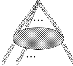
Figure 1: Gluonic Green’s function with operator insertion.

momentum we exclude the possibility of gauge variant operators emerging in the mixing matrix by ensuring the external gluons are on-shell. Thus for the external gluon $\tilde{A}^{a}_{\mu}(p)$ in momentum space, we multiply the Green’s function by $\epsilon_{\mu}(p)$, where $\epsilon_{\mu}$ are the spin-$1$ physical polarization vectors, and set $p_{\mu}p^{\mu}$ $=$ $0$ and $\epsilon_{\mu}(p)p^{\mu}$ $=$ $0$ for each such gluon. Consequently, when each operator is inserted the resulting output will involve a large number of terms involving different combinations of the factors $\epsilon_{i}\epsilon_{j}$, $p_{i}\epsilon_{j}$ ($i$ $\neq$ $j$) and $p_{i}p_{j}$ ($i$ $\neq$ $j$) where $1$ $\leq$ $i$,$j$ $\leq$ $n$. To resolve these into the operator basis we have computed the Feynman rules for each independent operator with the same number of gluon legs as the original operator and multiplied by $\epsilon_{\mu}(p)$ subjecting them to the same restrictions as above. The full set with arbitrary coefficients is compared with the operator output and the parameters fixed to cancel off all the one loop divergences. Given that Yang-Mills is renormalizable and that we have a basis set of operators then there is no redundancy or overconstraint in the computation of the parameters which are therefore uniquely determined.

To find the pole structure of each Green’s function we have chosen to compute using dimensional regularization where the space-time dimension is $d$ $=$ $4$ $-$ $2\epsilon$. The ultraviolet infinities will emerge as simple poles in $\epsilon$ at one loop. However, since we are working with Green’s functions which are at least $3$-point, (in the case of a two leg operator insertion), we cannot use the Mincer algorithm, [17], which applies only to $2$-point propagator type integrals. Moreover, if one uses massless propagators to compute, say, $4$-point or higher Green’s functions then there is a danger of obtaining spurious infrared infinities which in dimensional regularization are inseparable from the ultraviolet ones we seek. Instead we are forced to infrared regularize our one loop integrals by introducing a mass $m$ in the gluon propagator which acts as an infrared cutoff. Recently, a similar approach has been used in [18, 19] to systematically compute analogous Green’s functions for dimension five operators in QCD. Therefore, we use for our gluon propagator,

$$\frac{1}{(k^{2}+m^{2})}\left[\eta_{\mu\nu}~{}-~{}(1-\alpha)\frac{k_{\mu}k_{\nu}}{(k^{2}+m^{2})}\right]$$ (4.1)

where $m$ appears naturally as an infrared regularization. Moreover, we use a covariant gauge fixing with parameter $\alpha$. To ensure that our renormalization procedure with such a (gauge symmetry violating) propagator is valid, we have checked the full one loop renormalization of Yang-Mills using (4.1) and a mass independent renormalization scheme [20, 21]. This is important since the operators we are interested in are composite and therefore each field present in the operator will be renormalized requiring the wave function renormalization. For example,

$$\mbox{Tr}\left(D_{\mu}G_{\mbox{\footnotesize{o}}\,\nu\sigma}D^{\mu}G^{\nu\sigma}_{\mbox{\footnotesize{o}}}\right)~{}=~{}Z_{A}Z_{DGDG}\mbox{Tr}\left(D_{\mu}G_{\nu\sigma}D^{\mu}G^{\nu\sigma}\right)$$ (4.2)

where $A^{\mu}_{\hbox{\footnotesize{o}}}$ $=$ $Z_{A}^{\mbox{\small{$\frac{1}{2}$}}}A^{\mu}$ and the subscript, o, denotes the bare quantity. In this expression $Z_{A}$ is the usual gauge dependent gluon wave function renormalization and $Z_{DGDG}$ is related to the gauge independent anomalous dimension of the particular operator which we seek, if we ignore operator mixing for the moment. Therefore, by computing with a non-zero $\alpha$ we have a check which is that the operator renormalization constants which emerge must be gauge independent. Further, by first renormalizing Yang-Mills at one loop, this allows us to check that the Feynman rules we use are consistent. This is important since given the nature of the operators we are considering, whose Feynman rules can involve over four thousand terms, we have used a symbolic manipulation approach. The Feynman diagrams are generated with Qgraf, [22], and converted into a format recognizable by the language Form, [23]. We have written a programme to convert the Qgraf output into a typical Feynman integral with propagators and vertices substituted. The group theory for each graph is performed before the integrals are evaluated. This is achieved by reducing each diaagram to the corresponding vacuum bubble graph by systematically rewriting the propagators using the result, [18, 19],

$$\frac{1}{((k-p)^{2}+m^{2})}~{}=~{}\frac{1}{(k^{2}+m^{2})}~{}+~{}\frac{(2kp-p^{2})}{(k^{2}+m^{2})((k-p)^{2}+m^{2})}~{}.$$ (4.3)

This relation is exact but for mass regularized propagators all terms bar the first involve an external momentum in the numerator. If one continually repeats the substitution with the termination rule that $O(p^{4})$ terms, say, can be dropped due to Yang-Mills renormalizability, then the procedure will stop leaving only one loop massive vacuum bubbles which are easily calculated due to

$$\int_{k}\,\frac{1}{(k^{2}+m^{2})^{n}}~{}=~{}\frac{\Gamma(n-\mbox{\small{$\frac{1}{2}$}}d)}{(4\pi)^{\mbox{\small{$\frac{1}{2}$}}d}\Gamma(n)}(m^{2})^{\mbox{\small{$\frac{1}{2}$}}d-n}$$ (4.4)

for any $n$ $>$ $0$ where $\int_{k}$ $=$ $\int d^{d}k/(2\pi)^{d}$. We have implemented the above algorithm in Form, [23]. Finally, for operators which mix under the renormalization there will be extra terms in relations similar to (4.2). In general we have

$${\cal O}_{\mbox{\footnotesize{o}}\,i}~{}=~{}Z_{ij}{\cal O}_{j}$$ (4.5)

which gives the mixing matrix of anomalous dimensions

$$\gamma_{ij}(a)~{}=~{}\mu\frac{\partial~{}}{\partial\mu}\ln Z_{ij}~{}.$$ (4.6)

Having summarized our method and the general formalism, we now record our results. First, for the two independent dimension six operators there is no mixing and we find that

$$\gamma_{61}(a) = -~{}\frac{C_{A}}{2}a~{}+~{}O(a^{2})$$

$$\gamma_{62}(a) = -~{}\frac{11}{3}C_{A}a~{}+~{}O(a^{2})$$ (4.7)

where $a$ $=$ $g^{2}/(16\pi^{2})$ and the subscript on the anomalous dimension corresponds to the appropriate operator. The one loop expression for $\gamma_{61}(a)$ has been computed previously in [2, 8] and we note that we get consistency with both calculations which were performed in the background field gauge. For completeness we note that in both instances the dimension six operator which was considered were multiplied by powers of $a$. Including the respective contributions from the $\beta$-function allows one to compare the final expressions for the anomalous dimension of each operator. The anomalous dimension for ${\cal O}_{62}$ is new and is the same as the one loop Yang-Mills $\beta$-function, [24, 25].

For the dimension eight operators the full one loop mixing matrix of anomalous dimensions partitions into blocks defined by the number of legs on the operator. Therefore, we list only the entries in each of the blocks. First, for the single two leg operator

$$\gamma_{821,821}(a)~{}=~{}-~{}\frac{11}{3}C_{A}a~{}+~{}O(a^{2})~{}.$$ (4.8)

For three legs, we find

$$\gamma_{831,831}(a) = -~{}\frac{7}{6}C_{A}a~{}+~{}O(a^{2})~{}~{},~{}~{}\gamma_{831,832}(a)~{}=~{}\frac{1}{3}C_{A}a~{}+~{}O(a^{2})$$

$$\gamma_{832,831}(a) = O(a^{2})~{}~{},~{}~{}\gamma_{832,832}(a)~{}=~{}-~{}\frac{1}{2}C_{A}a~{}+~{}O(a^{2})$$ (4.9)

so that this sub-matrix is triangular at this order. For the four leg dimension eight operators the mixing matrix is further divided into sectors defined by the number of colour traces in the original operator. Thus, for the single trace operators we have

$$\gamma_{841,841}(a) = -~{}\left(\frac{25}{3}C_{F}~{}-~{}7C_{A}\right)a~{}+~{}O(a^{2})~{}~{},~{}~{}\gamma_{841,842}(a)~{}=~{}\frac{1}{3}C_{A}a~{}+~{}O(a^{2})$$

$$\gamma_{841,843}(a) = -~{}\left(16C_{F}~{}-~{}11C_{A}\right)a~{}+~{}O(a^{2})$$

$$\gamma_{841,844}(a) = \left(\frac{52}{3}C_{F}~{}-~{}11C_{A}\right)a~{}+~{}O(a^{2})$$

$$\gamma_{841,841a}(a) = \frac{23}{3}C_{F}a~{}+~{}O(a^{2})~{}~{},~{}~{}\gamma_{841,842a}(a)~{}=~{}\frac{2}{3}C_{F}a~{}+~{}O(a^{2})$$

$$\gamma_{841,843a}(a) = 16C_{F}a~{}+~{}O(a^{2})~{}~{},~{}~{}\gamma_{841,844a}(a)~{}=~{}-~{}\frac{52}{3}C_{F}a~{}+~{}O(a^{2})$$

$$\gamma_{842,841}(a) = \left(\frac{50}{3}C_{F}~{}-~{}8C_{A}\right)a~{}+~{}O(a^{2})~{}~{},~{}~{}\gamma_{842,842}(a)~{}=~{}-\frac{4}{3}C_{A}a~{}+~{}O(a^{2})$$

$$\gamma_{842,843}(a) = -~{}\left(\frac{56}{3}C_{F}~{}-~{}\frac{38}{3}C_{A}\right)a~{}+~{}O(a^{2})$$

$$\gamma_{842,844}(a) = \left(16C_{F}-10C_{A}\right)a~{}+~{}O(a^{2})$$

$$\gamma_{842,841a}(a) = -~{}\frac{2}{3}C_{F}a~{}+~{}O(a^{2})~{}~{},~{}~{}\gamma_{842,842a}(a)~{}=~{}-~{}16C_{F}a~{}+~{}O(a^{2})$$

$$\gamma_{842,843a}(a) = -~{}\frac{56}{3}C_{F}a~{}+~{}O(a^{2})~{}~{},~{}~{}\gamma_{842,844a}(a)~{}=~{}-~{}16C_{F}a~{}+~{}O(a^{2})$$

$$\gamma_{843,841}(a) = -~{}\left(12C_{F}~{}-~{}\frac{47}{6}C_{A}\right)a~{}+~{}O(a^{2})~{}~{},~{}~{}\gamma_{843,842}(a)~{}=~{}O(a^{2})$$

$$\gamma_{843,843}(a) = \left(\frac{34}{3}C_{F}~{}-~{}6C_{A}\right)a~{}+~{}O(a^{2})~{}~{},~{}~{}\gamma_{843,844}(a)~{}=~{}\left(\frac{14}{3}C_{F}-2C_{A}\right)a~{}+~{}O(a^{2})$$

$$\gamma_{843,841a}(a) = \frac{23}{3}C_{F}a~{}+~{}O(a^{2})~{}~{},~{}~{}\gamma_{843,842a}(a)~{}=~{}\frac{13}{3}C_{F}a~{}+~{}O(a^{2})$$

$$\gamma_{843,843a}(a) = -~{}\frac{34}{3}C_{F}a~{}+~{}O(a^{2})~{}~{},~{}~{}\gamma_{843,844a}(a)~{}=~{}-~{}\frac{14}{3}C_{F}a~{}+~{}O(a^{2})$$

$$\gamma_{844,841}(a) = \left(6C_{F}~{}-~{}\frac{19}{6}C_{A}\right)a~{}+~{}O(a^{2})~{}~{},~{}~{}\gamma_{844,842}(a)~{}=~{}-~{}C_{A}a~{}+~{}O(a^{2})$$

$$\gamma_{844,843}(a) = -~{}\left(\frac{14}{3}C_{F}~{}-~{}\frac{11}{3}C_{A}\right)a~{}+~{}O(a^{2})$$

$$\gamma_{844,844}(a) = -~{}\left(\frac{10}{3}C_{F}-\frac{13}{3}C_{A}\right)a~{}+~{}O(a^{2})$$

$$\gamma_{844,841a}(a) = \frac{5}{3}C_{F}a~{}+~{}O(a^{2})~{}~{},~{}~{}\gamma_{844,842a}(a)~{}=~{}-~{}\frac{23}{3}C_{F}a~{}+~{}O(a^{2})$$

$$\gamma_{844,843a}(a) = \frac{14}{3}C_{F}a~{}+~{}O(a^{2})~{}~{},~{}~{}\gamma_{844,844a}(a)~{}=~{}\frac{10}{3}C_{F}a~{}+~{}O(a^{2})~{}.$$ (4.10)

To simplify the expressions for the anomalous dimensions of the double colour trace operators we have introduced the intermediate operators

$${\cal O}_{8410} = f^{abe}f^{cde}G^{a}_{\mu\nu}G^{b\,\nu\sigma}G^{c}_{\sigma\rho}G^{d\,\rho\mu}$$

$${\cal O}_{8411} = f^{abe}f^{cde}G^{a}_{\mu\nu}G^{b}_{\sigma\rho}G^{c\,\mu\nu}G^{d\,\sigma\rho}$$ (4.11)

which are not independent as they are related by

$${\cal O}_{842}~{}=~{}{\cal O}_{841}~{}-~{}\mbox{\small{$\frac{1}{2}$}}T(R){\cal O}_{8411}~{}~{},~{}~{}{\cal O}_{844}~{}=~{}{\cal O}_{843}~{}+~{}\mbox{\small{$\frac{1}{2}$}}T(R){\cal O}_{8410}$$ (4.12)

where $\mbox{Tr}\left(T^{a}T^{b}\right)$ $=$ $T(R)\delta^{ab}$. Therefore, we have

$$\gamma_{845,845}(a) = \frac{22}{3}C_{A}a~{}+~{}O(a^{2})~{}~{},~{}~{}\gamma_{845,846}(a)~{}=~{}O(a^{2})~{}~{},~{}~{}\gamma_{845,847}(a)~{}=~{}O(a^{2})$$

$$\gamma_{845,848}(a) = O(a^{2})~{}~{},~{}~{}\gamma_{845,8410}(a)~{}=~{}-~{}28C_{A}a~{}+~{}O(a^{2})$$

$$\gamma_{845,8411}(a) = -~{}2C_{A}a~{}+~{}O(a^{2})$$

$$\gamma_{846,845}(a) = \frac{11}{6}C_{A}a~{}+~{}O(a^{2})~{}~{},~{}~{}\gamma_{846,846}(a)~{}=~{}O(a^{2})~{}~{},~{}~{}\gamma_{846,847}(a)~{}=~{}O(a^{2})$$

$$\gamma_{846,848}(a) = O(a^{2})~{}~{},~{}~{}\gamma_{846,8410}(a)~{}=~{}\frac{4}{3}C_{A}a~{}+~{}O(a^{2})$$

$$\gamma_{846,8411}(a) = \frac{11}{3}C_{A}a~{}+~{}O(a^{2})$$

$$\gamma_{847,845}(a) = -~{}\frac{1}{3}C_{A}a~{}+~{}O(a^{2})~{}~{},~{}~{}\gamma_{847,846}(a)~{}=~{}\frac{28}{3}C_{A}a~{}+~{}O(a^{2})$$

$$\gamma_{847,847}(a) = -~{}\frac{2}{3}C_{A}a~{}+~{}O(a^{2})~{}~{},~{}~{}\gamma_{847,848}(a)~{}=~{}-~{}8C_{A}a~{}+~{}O(a^{2})$$

$$\gamma_{847,8410}(a) = -~{}\frac{34}{3}C_{A}a~{}+~{}O(a^{2})~{}~{},~{}~{}\gamma_{847,8411}(a)~{}=~{}\frac{25}{3}C_{A}a~{}+~{}O(a^{2})$$

$$\gamma_{848,845}(a) = -~{}\frac{1}{6}C_{A}a~{}+~{}O(a^{2})~{}~{},~{}~{}\gamma_{848,846}(a)~{}=~{}\frac{14}{3}C_{A}a~{}+~{}O(a^{2})$$

$$\gamma_{848,847}(a) = -~{}4C_{A}a~{}+~{}O(a^{2})~{}~{},~{}~{}\gamma_{848,848}(a)~{}=~{}\frac{10}{3}C_{A}a~{}+~{}O(a^{2})$$

$$\gamma_{848,8410}(a) = -~{}\frac{2}{3}C_{A}a~{}+~{}O(a^{2})~{}~{},~{}~{}\gamma_{848,8411}(a)~{}=~{}\frac{11}{3}C_{A}a~{}+~{}O(a^{2})~{}.$$ (4.13)

Finally, for the total derivative operators we have

$$\gamma_{821t,821t}(a)~{}=~{}\gamma_{822t,822t}(a)~{}=~{}\gamma_{823t,823t}(a)~{}=~{}-~{}\frac{11}{3}C_{A}a~{}+~{}O(a^{2})~{}.$$ (4.14)

Having completed the full one loop renormalization we are now in a position to examine some of the results used in constructing the initial set of independent operators. For instance, the operators which involve a total derivative were related via the identities (2.21) and (2.22). By considering ${\cal O}_{62}$ these imply,

$$\mbox{Tr}\left(G_{\nu\sigma}D_{\mu}D^{\mu}G^{\nu\sigma}\right)~{}=~{}\partial_{\mu}\mbox{Tr}\left(G_{\nu\sigma}D^{\mu}G^{\nu\sigma}\right)~{}-~{}\mbox{Tr}\left(D_{\mu}G_{\nu\sigma}D^{\mu}G^{\nu\sigma}\right)$$ (4.15)

which was used in [3] but with the first term on the right omitted. However, one can compute the one loop renormalization of each operator in this result following the procedures we have discussed previously. In particular each operator is inserted in a gluon $2$-point function with a non-zero momentum flowing through the operator. It turns out that the total derivative operator of (4.15) has an anomalous dimension which is the same as ${\cal O}_{62}$ whilst their is no renormalization of the other operator. This is consistent since it is related to operators which vanish on the equation of motion or which involve higher legs and so has no two leg projection. Therefore, it would appear that omitting total derivative operators in calculations could lead to erroneous results.

5 Discussion.

We conclude with various remarks. First, we have computed the one loop anomalous dimensions of a set of linearly independent gauge invariant dimension six and eight operators for an arbitrary Lie group. Whilst we have reproduced results that had been derived previously we believe our calculation is more comprehensive since the systematic classification of all operators has been performed for the first time and operators which are total derivatives have been considered. Their effect cannot be neglected since operators are renormalized at non-zero momentum. Further, it transpires that there is an additional operator of dimension six which appears to have been omitted from phenomenological considerations. Second, our study has laid the foundation for extending the work in various directions. For instance, with the basis of independent physical operators it ought to be possible to renormalize these operators at two loops in Yang-Mills theory. Also, given the fact that several dimension eight operators at one loop have the same anomalous dimensions it would be interesting to see if the degeneracy is lifted at this order. Moreover, since there are more independent operators in the basis than would previously appear to have been considered it would be worthwhile to extend both the dimension six and eight bases to QCD when quark fields are included. Although at one loop previous analyses would seem to suggest a lack of mixing between the quark and gluon sectors the extension to two loops would also be worth pursuing since examination of the Feynman diagrams which are generated at two loops suggest that there will be mixing. In a related context the operators we have focused on have all been Lorentz scalars. Given the recent interest in $CP$-violation and the role dimension six operators play in probing physics beyond the standard model, [26], it will be important to repeat the one loop calculations for Lorentz pseudo-scalar operators. Indeed it would be interesting to see if an independent analogue of ${\cal O}_{62}$ exists. We hope to return to these issues in future work.

Acknowledgements. The author thanks Dr D.B. Ali and Prof. L. Dixon for useful discussions and the latter for pointing out references [9].

- [1] Y. Nambu & G. Jona-Lasinio, Phys. Rev. 122 (1961), 345.
- [2] A.Yu. Morozov, Sov. J. Nucl. Phys. 40 (1984), 505.
- [3] E.H. Simmons, Phys. Lett. B226 (1989), 132.
- [4] E.H. Simmons, Phys. Lett. B246 (1990), 471.
- [5] S.D. Joglekar & B.W. Lee, Ann. Phys. 97 (1976), 160.
- [6] S.D. Joglekar, Ann. Phys. 100 (1976), 395; Ann. Phys. 108 (1977), 233; Ann. Phys. 109 (1977), 210.
- [7] J.C. Collins, Renormalization (Cambridge University Press, 1984).
- [8] S. Narison & R. Tarrach, Phys. Lett. B125 (1983), 217.
- [9] L.J. Dixon & Y. Shadmi, Nucl. Phys. B423 (1994), 3; Nucl. Phys. B452 (1995), 724.
- [10] M. Beneke, V.M. Braun & N. Kivel, Phys. Lett. B404 (1997), 315.
- [11] J. Kodaira, Nucl. Phys. B165 (1980), 129.
- [12] S.A. Larin, Phys. Lett. B303 (1993), 113.
- [13] T. van Ritbergen, J.A.M. Vermaseren & S.A. Larin, Phys. Lett. B400, 327; T. van Ritbergen, A.N. Schellekens & J.A.M. Vermaseren, Int. J. Mod. Phys. A14 (1999), 41.
- [14] R. Hamberg & W.L. van Neerven, Nucl. Phys. B379 (1992), 143.
- [15] W. Furmanski & R. Petronzio, Phys. Lett. B97 (1980), 437; E.G. Floratos, D.A. Ross & C.T. Sachrajda, Nucl. Phys. B152, (1979), 493.
- [16] J.C. Collins & R.J. Scalise, Phys. Rev. D50 (1994), 4117; B.W. Harris & J. Smith, Phys. Rev. D51 (1995), 4550.
- [17] S.G. Gorishny, S.A. Larin, L.R. Surguladze & F.K. Tkachov, Comput. Phys. Commun. 55 (1989), 381; S.A. Larin, F.V. Tkachov & J.A.M. Vermaseren, “The Form version of Mincer”, NIKHEF-H-91-18.
- [18] M. Misiak & M. Münz, Phys. Lett. B344 (1995), 308.
- [19] K.G. Chetyrkin, M. Misiak & M. Münz, Nucl. Phys. B518 (1998), 473.
- [20] D.J. Gross & F.J. Wilczek, Phys. Rev. Lett. 30 (1973), 1343.
- [21] H.D. Politzer, Phys. Rev. Lett. 30 (1973), 1346.
- [22] P. Nogueira, J. Comput. Phys. 105 (1993), 279.
- [23] J.A.M. Vermaseren, “Form” version , (CAN Amsterdam, 1992).
- [24] H. Kluberg-Stern & J.B. Zuber, Phys. Rev. D12 (1975), 467.
- [25] J.C. Collins, A. Duncan & S.D. Joglekar, Phys. Rev. D16 (1977), 438.
- [26] S. Weinberg, Phys. Rev. Lett. 63 (1989), 2333.