Non-abelian Topological Strings and Metastable States in Linear Sigma Model

Abstract

Non-abelian (NA) topological string defects exist in QCD with the spontaneous chiral symmetry breaking $U(N_{f})_{L}\times U(N_{f})_{R}\to U(N_{f})_{V}$. Anomaly effects lead to domain walls connected to these strings. In the framework of linear sigma model we find the configuration of these defects. Also we show that in this model metastable $CP$ violating vacuua exist. Strings as well as extended regions of metastable vacuua may form during the chiral transition which could have interesting effects.

I Introduction

QCD with $N_{f}$ flavors of massless quarks possesses the chiral symmetry $U(N_{f})_{L}\times U(N_{f})_{R}$. The generators of its diagonal subgroup $U(N_{f})_{V}$ are parity invariant while the parity-odd generators give the axial transformations $U(N_{f})_{A}$. (The latter do not form a group.) For low energy and temperatures the axial vector part of this symmetry suffers spontaneous symmetry breakdown (SSB), this is indicated by $U(N_{f})_{V}\times U(N_{f})_{A}\longrightarrow U(N_{f})_{V}$ [1]. This creates $N_{f}^{2}$ massless pseudoscalar Goldstone bosons known as mesons. However in the real world, chiral symmetry is explicitly broken because of non-zero quark masses. This makes the pseudoscalar mesons massive. Even in the chiral limit, anomaly effects break the $SU(N_{f})_{V}$-invariant axial $U(1)$ subgroup $U(1)_{A}\subset U(N_{f})_{A}$ to $Z_{N_{f}}$ [2] making the $\eta^{\prime}$ meson heavier compared to other mesons. Finite temperature lattice QCD studies show that chiral symmetry (but for $U(1)_{A}$ of course which is only effectively restored) is restored at temperatures, $T$ larger than a critical value $T_{\chi}$. Such chirally symmetric phase of matter is believed to have existed in the early Universe. The matter in the initial stages of the fire ball produced in heavy ion collisions is likely to be in the chirally symmetric phase. To see such a phase transition in laboratory is one of the motivations of heavy-ion collision experiments.

The chirally symmetric and broken phases of QCD are characterized by an order parameter (OP) which is the quark-antiquark condensate known as the chiral condensate $\Phi$. It is an $N_{f}\times N_{f}$ matrix at each $x$. In the chiral symmetry limit (with no anomaly), all possible values of $\Phi$ constitute the order parameter space (OPS). In the broken symmetry phase instead, it is diffeomorphic to $U(N_{f})$. $U(N_{f})$ as the OPS allows for the existence of “abelian” as well as “non-abelian” topological string defects. Brandenberger et al.[3] first studied the formation of “abelian” strings due to SSB of the $U(1)_{A}$ part of chiral symmetry. In [3] it was argued that these string defects will exist as long as the anomaly effects are small and will decay as the anomaly becomes substantial. In a previous work we have considered the effects of anomaly on abelian strings [4]. We have argued that abelian strings will exist in the presence of anomaly with the typical structure of $N_{f}$ domain walls connected to the string. Now, a closer look at the full OPS=$U(N_{f})$ shows that an additional class of topological defects, known as non-abelian (NA) strings can also exist, as the arguments in ref.[5] for example show. Note that here we use the phrase ”non-abelian strings” in same way as the phrase ”non-abelian monopoles” [5, 6] are used and not in the sense that $\pi_{1}(OPS)$ is non-abelian. Here we find and discuss numerical solutions for these NA strings and note the important differences between the NA and abelian strings. Also we show that in the linear sigma model we employ, metastable vacua exist at zero temperature. Such metastable states have been found to exist in the non-linear sigma model [7] before, but for temperatures close to the deconfinement and/or chiral phase transition.

In the next section we briefly discuss how the non-abelian string defects arise from the topological structure of the OPS=$U(N_{f})$ during the SSB of chiral symmetry. In section III we find the numerical profiles for the NA strings using the linear sigma model Lagrangian [8]. In sec. IV we show existence of metastable CP violating states in the above model. In section V we conclude with some speculative remarks on the formation of these string defects and metastable states during and/or after the chiral phase transition.

II Non-abelian strings in QCD

Topological defects are usually formed in phase transitions associated with SSB with non-trivial OPS. The type of defects formed depends on the dimension $n$ of physical space and the topology of the OPS. When the OPS after SSB is discrete, the topological defects are domain walls in 3-dimensional (3-D) physical space. When the OPS after SSB is a circle the defects are vortices in 2-D and strings in 3-D physical spaces. Monopoles arise in 3-D when the OPS after SSB is a 2-sphere ($S^{2}$). For an introduction to and review of topological defects, see [9]. For our discussion we need to know only about the string defects. In the following we discuss briefly about how string defects arise.

Topological string defects arise when there exist non-trivial loops in the OPS, for example when it is a circle. A loop going around the circle $k$ times cannot be smoothly shrunk to a point or cannot be smoothly deformed to another loop going $l\neq k$ times around the circle. So there exist non-trivial loops, characterized by windings, on the circle. There is a close connection between the non-trivial loops and the string defects in physical space, see Fig.1. A string defect of winding $k$ corresponds to a non-trivial loop winding $k$ times around a circle, not contractible to a point in the OPS, as a loop $\bf{l}$ around the string is traversed once in physical space. In Fig. 1 we show an example of winding number 1 string defect for the case of a complex scalar field $\Psi$ with real and imaginary parts $\Psi_{1}$ and $\Psi_{2}$ when SSB is of $U(1)$. The figure on the left of Fig.1 shows the typical effective potential for such a case. The minima $\bf{\it{M}}$ of the potential is a circle with radius $|\Psi|$. The configuration $\Psi$ of the string on the loop $\bf{l}$ (on $xy$-plane) around the string core is shown on the right. Magnitude of $\Psi$ is represented by the length of the vectors and the phase by the angle $\theta$ these vectors make with the positive $x$-axis. As one goes around $\bf{l}$ once $\Psi$ on it traces a complete winding on $\bf{\it{M}}$. However, the configuration of $\Psi$ could have been such that it winds $k$-times (for a winding number $k$ string) around $\bf{\it{M}}$ for a single loop on $\bf{l}$.

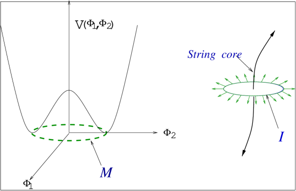
FIG. 1.: On the left is the effective potential for SSB of $U(1)$. The vacua are represented by the dashed circle. On the right is shown the configuration of the complex scalar field on the loop ${\it{{\bf l}}}$ around the string core.

The stability of the string defect is purely due to topological reasons. The total variation $\Delta\theta$ of $\theta$ around $\bf{l}$ can have only discrete values, namely integral multiples $2\pi k$ of $2\pi$. So by smooth changes of $\Psi$ on $\bf{l}$, one can not change $\Delta\theta$. Also by smoothly shrinking or enlarging $\bf{l}$, such that it does not cross $\Psi=0$ when $\theta$ becomes undefined, one cannot change $\Delta\theta$ if the underlying $\Psi$ is continuous. On the other hand if $\bf{l}$ can be shrunk to a point ( keeping $\Psi$ continuous and non-zero except perhaps at that point, and $\Delta\theta$ fixed in the process), then either $k=0$ or $\Psi$ must vanish at that point as it is continuous. By definition, $k\neq 0$ when there is a string (defect). The point where $\Psi=0$ when $k\neq 0$ is the core of the string. Strings in 3-D are either infinitely long or exist in loops. As strings have non-zero string tension, a string loop is unstable to shrinking.

It is important to note that string defects arise because one can have loops with non-trivial winding on $\bf{\it{M}}$ which is a circle in the above example. Such non-trivial loops exist in $U(N_{f})$ which is the OPS after SSB of chiral symmetry. Thus let $T_{a}$ (a $\epsilon\{1,N_{f}^{2}-1\}$) be the $SU(N_{f})$ Lie algebra generators (the analogues of the Gell-mann matrices $\lambda_{a}$) and

$$T_{0}=\sqrt{2\over N_{f}}\bf{1}.$$ (1)

Noting that

$$T_{N_{f}^{2}-1}=\left({2\over N_{f}(N_{f}-1)}\right)^{1\over 2}\left(\begin{array}[]{cccccc}1&&&&&\\ &1&&&&\\ &&.&&&\\ &&&.&&\\ &&&&1&\\ &&&&&1-N_{f}\end{array}\right),$$ (2)

a particular non-abelian string configuration is

$$M(\theta)=e^{i{\theta\over N_{f}}\left[N_{f}(N_{f}-1)\over 2\right]^{1\over 2}T_{N_{f}^{2}-1}}e^{-i{\theta\over N_{f}}\left[N_{f}\over 2\right]^{1\over 2}T_{0}}$$ (3)

where $\theta$ is the angle on $\bf{{l}}$. The first factor is an open curve in $SU(N_{f})$ from $\bf{1}$ to its center $e^{i{2\pi\over N_{f}}}\bf{1}$. The second is an open curve in the center $U(1)$ of $U(N_{f})$ from $\bf{1}$ to $e^{-i{2\pi\over N_{f}}}\bf{1}$. On taking their product as in the above equation, the values at $\theta=2\pi$ multiply to $\bf{1}$ giving a closed string. The powers $M(\theta)^{N}$ ($N\in Z\backslash\{0\}$) and their (continuous) deformations produce all possible strings, the deformations not changing their topological types. The beginning and end points of the non-abelian and abelian factors remain fixed during these deformations.

Note that in $M(\theta)^{nN_{f}}$ ($n\in Z\backslash\{0\}$), the non-abelian factor

$$e^{in\theta\left[N_{f}(N_{f}-1)\over 2\right]^{1\over 2}T_{N_{f}^{2}-1}}$$ (4)

is a closed loop in $SU(N_{f})$. Such loops can be deformed to a point as the first homotopy group of $SU(N_{f})$, $\pi_{1}(SU(N_{f}))$ is $0$. Thus $M(\theta)^{nN_{f}}$ gives the abelian strings. In other words, the elementary strings are given by $M(\theta)$ and $M(\theta)^{-1}$. Note that by construction $M(\theta)^{n}$ gives a loop winding $n$ times. Consider the loop given by

$$M^{\prime}(\theta)=e^{i{\theta\over N_{f}}\left[N_{f}(N_{f}-1)\over 2\right]^{1\over 2}T_{N_{f}^{2}-1}}e^{i{\theta(N_{f}-1)\over N_{f}}\left[N_{f}\over 2\right]^{1\over 2}T_{0}},$$ (5)

for which the open curve in $SU(N_{f})$ remains the same as that of $M(\theta)$, but one traverses the two end points in $U(1)$ in an anti-clockwise direction. This loop is actually homotopic to the loop given by $M(\theta)^{1-N_{f}}$. That is to say, there is a string loop homotopic to that of $M(\theta)^{1-N_{f}}$ which gives the string configuration of (4).

In the above we have considered SSB of chiral symmetry. However in the real world this symmetry is explicitly broken due to quark masses, and also the $U(1)_{A}$ part of $U(N_{f})_{A}$ is broken down to $Z_{N_{f}}$ due to axial anomaly and instanton effects.The effect of anomaly changes the usual cylindrical structure of the string creating domain walls connecting to the string core. In the case of abelian strings, for $N_{f}=3$, the string gets connected to three domain walls [4]. In the case of elementary NA strings the number of domain walls can be either one or two as we explain in the next section. The effect of quark masses makes the string configurations non-static. However the string defects are stable against small fluctuations and can only decay due to annihilation with other defects with opposite windings.

In the next section we will numerically find the configuration of the elementary non-abelian strings for the case of $N_{f}=3$. For our calculations we use the linear sigma model Lagrangian considered in ref.[8]. Numerically it is easier to find the static configurations. Because of this we work in the chiral limit which allows for static solutions.

III Configurations of the non-abelian string

To find the field configurations for the non-abelian strings we consider the following $U(3)_{L}\times U(3)_{R}$ linear sigma model for $3$ quark flavors [8, 10],

$${\cal L}(\Phi) = {\rm Tr}\left(\partial_{\mu}\Phi^{\dagger}\partial^{\mu}\Phi-m^{2}\,\Phi^{\dagger}\Phi\right)-\lambda_{1}\left[{\rm Tr}\left(\Phi^{\dagger}\Phi\right)\right]^{2}-\lambda_{2}{\rm Tr}\left(\Phi^{\dagger}\Phi\right)^{2}$$ (6)

$$+ c\left[{\rm Det}\left(\Phi\right)+{\rm Det}\left(\Phi^{\dagger}\right)\right]+{\rm Tr}\left[H(\Phi+\Phi^{\dagger})\right]\,\,,$$ (7)

where we take $c>0$ for specificity. $\Phi$ is a complex $3\times 3$ matrix of fields of the scalar and pseudoscalar mesons:

$$\Phi=T_{a}\,\phi_{a}=T_{a}\,(\sigma_{a}+i\pi_{a}).$$ (8)

The field $\Phi$ transforms under the chiral transformation $U(3)_{L}\times U(3)_{R}$ as

$$\Phi\longrightarrow U_{\ell}\,\Phi\,U_{r}^{\dagger}\,\,\,,\,\,\,\,U_{\ell,r}\equiv\exp\left(i\,\omega_{\ell,r}^{a}\,T_{a}\right)\,\,.$$ (9)

One can rewrite the infinitesimal left-right transformations in terms of vector-axial vector transformations with parameters $w^{a}_{V,A}=(w^{a}_{l}\pm w^{a}_{r})/2$. The infinitesimal form of the $U(3)_{L}\times U(3)_{R}$ symmetry transformation (9) is

$$\Phi\longrightarrow\Phi+i\,\omega_{V}^{a}\,\left[T_{a},\Phi\right]+i\,\omega_{A}^{a}\,\left\{T_{a},\Phi\right\}\,\,.$$ (10)

$\Phi$ is a singlet under the $U(1)_{V}$ transformations associated with $exp(iw^{0}_{V}T^{0})$. In QCD, they give rise to a conserved charge identified with the baryon number.

In the above model the determinant term takes into account the instanton effect which explicitly breaks the $U(1)_{A}$ symmetry [10]. It is not clear whether such a term can be justified for high temperatures, because vanishing $\Phi$ makes the instanton effects to disappear [11], though lattice results show that $U(1)_{A}$ is effectively restored at slightly higher temperatures [12] than the temperature at which $SU(N)_{A}$ symmetry is restored. The last term where ($H=T_{a}h_{a}$, $h_{a}=$ constants) is due to non-zero quark masses. When $c=H=0$ and $\lambda_{1}>0$, and $\lambda_{2}>0$, the Lagrangian has a global symmetry $U(N_{f})_{V}\times U(N_{f})_{A}$ for $m^{2}>0$. For $m^{2}<0$ the axial symmetry $U(N_{f})_{A}$ is spontaneously broken to identity and the OPS is $U(N_{f})$. This results in $N_{f}^{2}$ Goldstone bosons. For $N_{f}=3$ these Goldstone bosons are the $\pi$’s, $K$’s, $\eta$ and $\eta^{\prime}$. However when just $c\neq 0$, the $U(1)_{A}$ is further broken to $Z_{3}$ by the axial anomaly. $U(3)_{A}$ symmetry is, in addition, explicitly broken by non-zero quark masses. Also $SU(3)_{V}$ is explicitly broken due to the difference in $u,d$, and $s$ quark masses giving rise to splitting in the meson masses.

In order to find the static non-abelian string configurations we take $H$ to be zero. Even when $H=0$, not all the non-abelian strings are static in the presence of anomaly just like the abelian string. To illustrate this we consider the NA string corresponding to the non-trivial loop $M(\theta)$ [with $N_{f}=3$] on $U(3)$. Scaling $M(\theta)$ by the vacuum $\Phi_{0}={\sigma_{0}\over\sqrt{6}}\bf{1}$, we get the loop in the space of fields $\Phi$ to be

$$\Phi(\theta)={\sigma_{0}\over\sqrt{6}}M(\theta)={1\over\sqrt{6}}\left(\begin{array}[]{ccc}\sigma_{0}&0&0\\ 0&\sigma_{0}&0\\ 0&0&\sigma_{0}e^{-i\theta}\end{array}\right).$$ (11)

As only the last diagonal component of $\Phi$ varies with $\theta$, the anomaly contribution to the effective Lagrangian from such field variation is

$${c\over 3\sqrt{6}}\sigma_{0}^{3}cos\theta.$$ (12)

For such a term, the ground state prefers the unique value $cos\theta=1$. Because of this, the $\theta$ distribution around the string will not be symmetric. In most of the region around the string, $\theta$ will take the value $0$ which minimizes the potential energy term (10). Non-zero $\theta$ values will be confined to a wall-like region. Because of non-zero surface tension of the wall, motion of the string towards the wall decreases the energy of the configuration. So one will not have static solutions in this case.

On the other hand, the loop corresponding to $M(\theta)^{n}$ in OPS gives rise to a string configuration with $|n|$ domain walls. This configuration is static as the motion of the string along any domain wall does not decrease the energy of the configuration. To find out the details of one such NA string configuration, we consider $N_{f}=3$ and $n=-2$. Here $M(\theta)^{-2}$ gives a loop homotopic to the loop of $M^{\prime}(\theta)$. For $N_{f}=3$, $M^{\prime}(\theta)$ is given by $exp(i\theta T_{s})$ where $T_{s}$ is

$$T_{s}=\left(\begin{array}[]{ccc}1&0&0\\ 0&1&0\\ 0&0&0\end{array}\right).$$ (13)

The corresponding loop in the space of fields $\Phi$ is from

$$\Phi(\theta)={\sigma_{0}\over\sqrt{6}}M^{\prime}(\theta)={1\over\sqrt{6}}\left(\begin{array}[]{ccc}\sigma_{0}e^{i\theta}&0&0\\ 0&\sigma_{0}e^{i\theta}&0\\ 0&0&\sigma_{0}\end{array}\right).$$ (14)

Writing $\sqrt{3\over 2}({\phi_{1}+i\phi_{2}})$ for $\sigma_{0}e^{i\theta}$, the effective Lagrangian for such a $\Phi$ deduced from (6), with $\lambda_{1}=\lambda$, $\lambda_{2}=0$ and $H=0$, is given by

$${\cal L} = {1\over 2}\partial_{\mu}\phi_{1}\partial^{\mu}\phi_{1}+{1\over 2}\partial_{\mu}\phi_{2}\partial^{\mu}\phi_{2}-{\cal V}(\phi_{1},\phi_{2}),$$ (15)

where

$${\cal V}(\phi_{1},\phi_{2}) = {m^{2}+{\lambda\sigma_{0}^{2}\over 3}\over 2}\,\left(\phi_{1}^{2}+\phi_{2}^{2}\right)+{\lambda\over 4}\left(\phi_{1}^{2}+\phi_{2}^{2}\right)^{2}$$ (16)

$$- {c\sigma_{0}\over 2\sqrt{6}}\left(\phi_{1}^{2}-\phi_{2}^{2}\right)+{m^{2}\over 6}\sigma_{0}^{2}+{\lambda\over 36}\sigma_{0}^{4}.$$ (17)

The values of the parameters in the above equation are $\lambda=53.5322$, $c=6685.19MeV$ and $m^{2}=-(591.256MeV)^{2}$. For these values of the parameters we get $\sigma_{0}=110.23MeV$, the sigma meson mass $m_{\sigma}=1000MeV$, and the $\eta^{\prime}$ mass $m_{\eta^{\prime}}=950MeV$. Note that the anomaly term in ${\cal V}$ expressed in $\theta$ is $-{c\sigma_{0}/2\sqrt{6}}cos(2\theta)$ for which $\theta=0$ and $\theta=\pi$ are degenerate. This leads to a string configuration attached to 2 domain walls. In the following we will find the approximate numerical profile of the string associated with $M^{\prime}(\theta)$.

Considering the string along the $z$-direction, $\phi_{i}$ for the static string satisfy the following field equations:

$$\nabla^{2}\phi_{1}={\partial{{\cal V}(\phi_{1},\phi_{2})}\over\partial{\phi_{1}}},$$ (18)

$$\nabla^{2}\phi_{2}={\partial{{\cal V}(\phi_{1},\phi_{2})}\over\partial{\phi_{2}}},$$ (19)

where $\nabla^{2}={\partial^{2}\over\partial x^{2}}+{\partial^{2}\over\partial y^{2}}$. Since in the presence of anomaly, the string profile is non-cylindrical, one has to find the solution by an energy minimization technique. For this we consider an initial cylindrical configuration with $\dot{\phi_{i}}=0$ at $t=0$ and evolve it with the field equations derived from Eq.(6) with a dissipative term:

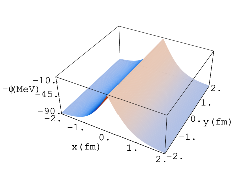
FIG. 2.: Configuration of the string for $c=6685.19MeV$ and $H=0$. Figure on the left gives $-\sqrt{\phi_{1}^{2}+\phi_{2}^{2}}\equiv-\phi$ and figure on the right gives the vector field plot of the full field $\phi_{1}(\vec{r})+i\phi_{2}(\vec{r})$.

$${d^{2}\phi_{1}\over dt^{2}}+\alpha{d\phi_{1}\over dt}-\nabla^{2}\phi_{1}=-{\partial{{\cal V}(\phi_{1},\phi_{2})}\over\partial{\phi_{1}}}$$ (20)

$${d^{2}\phi_{2}\over dt^{2}}+\alpha{d\phi_{2}\over dt}-\nabla^{2}\phi_{2}=-{\partial{{\cal V}(\phi_{1},\phi_{2})}\over\partial{\phi_{2}}}.$$ (21)

Here $\alpha$ is the dissipation coefficient. The dissipation term has been used to converge the initial configuration (the circular configuration, which is not the correct configuration in the presence of the anomaly) to the approximate configuration of the string connected to domain walls. Once the evolution is done for a sufficiently long time, the configuration does not evolve with time even after the dissipation is switched off, which suggests that the configuration is more or less static and so an approximate solution. On evolving the initial cylindrically symmetric configuration with the above equations, the domain walls connected to the string develop. In the numerical work, we considered the $\eta^{\prime}$ mass to be the experimental value $m_{\eta^{\prime}}\sim 950MeV$ and set other pseudoscalar meson masses to zero. In FIG.2 we show the configuration of the string with the domain walls joined to it. In the left figure we plot $-\sqrt{\phi_{1}^{2}+\phi_{2}^{2}}$, and in the right plot the vector field of $\Phi({\bf\vec{r}})=(\phi_{1}(\vec{r}),\phi_{2}(\vec{r}))$. The magnitude of the field is proportional to the length of the vectors and the angle these vectors make with +ve $x$-axis is the phase. Clearly there is no symmetric distribution of the phase around the string. In the core of the string the full chiral symmetry associated with $T_{s}$ is restored. That is because in the string core, as we explain below, $\Phi$ becomes $diag(0,0,constant)$ which is invariant under transformations generated by $T_{s}$. Although the field configuration has the structure of domain wall, the symmetry is restored only in the core of the string. It is not clear if it is the string tension or the surface tension of the domain wall that will dominate the dynamics when these configurations are formed after the chiral transition.

In the absence of anomaly the NA and abelian string configurations [4] look superficially similar. But there are crucial differences. For in the core of the abelian string all the components of $\Phi$ vanish and so the full chiral symmetry is restored. This is because the phase of all components of $\Phi$ change by $2\pi n$ ($n$ being a non-zero integer) as one goes round an abelian string obliging all these components to vanish at the core of the string. But for a NA string one or more components of $\Phi$ need not change in phase as the string is encircled, and hence need not vanish in the string core. As a consequence the full chiral symmetry associated with a particular linear combination of $T_{0}$ and $T_{N_{f}^{2}-1}$ for which the nonzero components are singlets is restored. The other difference is as we have mentioned above, for $c\neq 0$, the elementary abelian string for $N_{f}$ flavours is connected to $N_{f}$ domain walls while the elementary NA strings (associated with $M(\theta)$ and $M(\theta)^{-1}$) are connected to $1,2,...,N_{f}-1$ domain walls. (But note that $M^{\prime}(\theta)$ has two domain walls.)

IV Metastable states in $U(3)\times U(3)$ linear sigma model

As we have mentioned, in the chiral limit, anomaly breaks $U(1)_{A}$ to $Z_{3}$ in 3 flavour QCD. This leads to a set of discrete ground states related by discrete transformations of $U(3)$. It is simple to find out the ground states in the chiral limit. Let us consider the effective potential in Eq.5,

$${\cal V}(\Phi) = {\rm Tr}\left(m^{2}\,\Phi^{\dagger}\Phi\right)+\lambda_{1}\left[{\rm Tr}\left(\Phi^{\dagger}\Phi\right)\right]^{2}+\lambda_{2}{\rm Tr}\left(\Phi^{\dagger}\Phi\right)^{2}$$ (22)

$$- c\left[{\rm Det}\left(\Phi\right)+{\rm Det}\left(\Phi^{\dagger}\right)\right]-{\rm Tr}\left[H(\Phi+\Phi^{\dagger})\right]\,\,.$$ (23)

In the chiral limit when $H=0$, one can choose the ground states to be of the form $\Phi_{0}=\bar{\sigma_{0}}{T_{0}}/\sqrt{2}$. When the anomaly is also absent, $c=0$, and all $U(3)_{A}$ rotations of $\Phi_{0}$ cost no energy. For $c\neq 0$, only a few discrete axial rotations do not change the potential energy. Thus there are a few ground states. Some of the ground states are obtained by the discrete rotations $U\Phi_{0}U$, where $U=exp(-i\theta_{1}/2)$, with $\theta_{1}={2\pi\over 3},{4\pi\over 3}$. Also one can choose $U=exp(-i\theta_{2}T/2)$, where $T$ is a linear combinations of $T_{a}$’s and $T_{0}$, for example $T_{s}$ in Eq.11. For $T=T_{s}$, $\theta_{2}=\pi$ gives another ground state. All these ground states, except $\Phi_{0}$, will have non-zero $U(1)_{A}$ phase giving rise to $CP$ violating effects [7].

For the full potential (18), these states with $\theta_{1,2}\neq 0$ will be of higher energy. Still these states with differing values of $\theta_{1,2}$ are separated by energy barriers. When the quark mass is switched on, only one of these states becomes the true ground state. However, for small quark masses, the barrier between the ground state and other states may remain appreciable making them metastable. Because of their $CP$ violating nature it is interesting to check if such metastable states can exist after including the effects of the meson masses and their splittings. In the non-linear sigma model [7] such states are known to appear for temperatures close to the deconfinement transition. Here we now show that such states exist also in the linear sigma model at zero temperature. Since these are due to effects of anomaly we expect that they will survive as long as anomaly effects are significant.

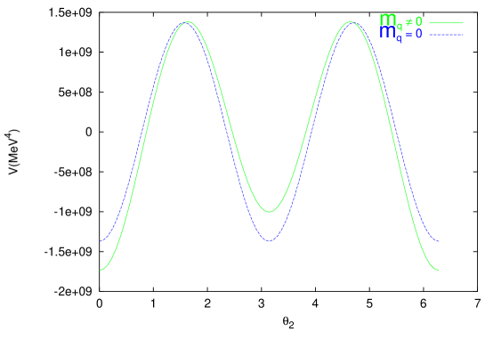
FIG. 3.: $\theta_{2}$ dependence of the potential energy for $m_{q}=0$ and $m_{q}\neq 0$.

In order to find metastable states, we took the values of the parameters in Eq. (18) from [8] which give an approximate description of meson masses and their splittings. The ground state is $\Phi_{0}=\bar{\sigma_{0}}{T_{0}}/\sqrt{2}+\bar{\sigma_{8}}T_{8}$, where $\bar{\sigma_{0}}\sim 130MeV$ and $\bar{\sigma_{8}}\sim-24MeV$ while $H$ is $h_{0}{T_{0}}/\sqrt{2}+h_{8}T_{8}$, where $h_{0}=(286.094MeV)^{3}$ and $h_{8}=-(310.960MeV)^{3}$. Finally $\lambda_{1}=1.4$ and $\lambda_{2}=46.484$. In order to see possible metastable states, we fix $\sigma_{0}$ and $\sigma_{8}$ and plot the $\theta_{1,2}$ dependence of the potential energy. In case there is a local minimum for non-zero $\theta_{1,2}$, we then minimize ${\cal V}(\Phi)$ relaxing $\bar{\sigma_{0}}$ and $\bar{\sigma_{8}}$ fixing $\theta_{1,2}$. If the new $\bar{\sigma_{0}}$ and $\bar{\sigma_{8}}$ are close to their initial values, then it implies the existence of metastable states. We find no metastable states for non-zero $\theta_{1}$, so there exists no metastable state with purely $U(1)_{A}$ phase. For $\theta_{2}$ there exists a metastable state at $\theta_{2}=\pi$. In Fig. 3 we plot the $\theta_{2}$ dependence of the potential energy for $m=0$ and $m_{q}\neq 0$. The figure clearly shows that there is a local minimum at $\theta_{2}=\pi$ for $m_{q}\neq 0$. Fixing $\theta_{2}$ at $\pi$ we minimize ${\cal V}(\Phi)$ varying $\bar{\sigma_{0}}$ and $\bar{\sigma_{8}}$. The new values are $\bar{\sigma_{0}}\sim 120MeV$ and $\bar{\sigma_{8}}=-28MeV$ indeed very close to the initial values.

Conclusions

In summary, we have numerically found an approximate static solution of a non-abelian string (domain wall) in the SSB of $U(N_{f})\times U(N_{f})\rightarrow U(N_{f})$ in the linear sigma model. Also we have shown that metastable states exist in this model for realistic quark masses. Abelian and non-abelian extended regions in metastable vacua may form during the chiral transition ocurring in the early stages of heavy-ion collisions as well as in the early Universe. However, formation of strings and large metastable domains are complementary as formation of the one suppresses the formation of other. More the number of uncorrelated domains, more are the number of strings, with less probability for an extended domain in a metastable state.

Acknowledgments

This work was supported by DOE and NSF under contract numbers DE - FG02 - 85ERR 40231 and INT - 9908763 and by BMFB (Germany) under grant 06 BI 902. We have benefited greatly from discussions with A. M. Srivastava.

REFERENCES

- [1] C. Vafa and E. Witten, Nucl. Phys. B234, 173 (1984); Commun. Math. Phys. 95, 257 (1984).
- [2] G. ’t Hooft, Phys. Rev. Lett. 37, 8 (1976); Phys. Rev. D 14, 3432 (1976).
- [3] X. Zhang, T. Huang, and R. H. Brandenberger Phys. Rev. D58 027702, (1998); R. H. Brandenberger, and X. Zhang Phys. Rev. D59 081301, (1999).
- [4] A. P. Balachandran and S. Digal, hep-ph/0108086 (Int. J. Mod. Phys. A, in press).
- [5] A. P. Balachandran, G. Marmo, N. Mukunda, J. S. Nilsson, E. C. G. Sudarshan, and F. Zaccaria, Phys. Rev. Lett 50, 1553 (1983); ibid Phys, Rev. D29, 2919 (1984); ibid Phys. Rev. D29, 2936 (1984); P. Nelson and A. Manohar, Phys.Rev.Lett. 50, 943 (1983); A. Abouelsaood, Phys. Lett. B125, 467 (1983) and references therein.
- [6] G. ’t Hooft, Nucl. Phys. B79,276 (1974); A. M. Polyakov, Pis’ma JETP 20, 430 (1974).
- [7] D. Kharzeev, R. D. Pisarski and M. H.G. Tytgat, Phys. Rev. Lett. 81 512, (1998).
- [8] J. T. Lenaghan and D. H. Rischke, Phys. Rev. D62,085008, (2000).
- [9] N. D. Mermin, Rev. Mod. Phys. 51, 591 (1979); A. Vilenkin and E. P. S. Shellard, “ Cosmic strings and other topological defects”, (Cambridge University Press, Cambridge, 1994).
- [10] C. Rosenzweig, J. Schechter, C. G. Trahern, Phys. Rev. D21, 3388, (1980); A. Aurilia, Y. Takahashi, and P. K. Townsend, Phys. Lett. B95, 265, (1980).
- [11] R. D. Pisarski and F. Wilczek, Phys. Rev. D29, 338, (1984).
- [12] B. Alles, M. D’Elia, and A. Di Giacomo, Phys.Lett. B483, 139, (2000).