Measuring the Spin of Invisible Massive Graviton Excitations at Future Linear Colliders

Abstract:

We consider the production process $e^{-}e^{+}\to G\gamma$ of invisible gravitons ($G$) at future linear colliders. We discuss whether the angular distribution of the photon ($\gamma$) can be used to measure the spin of the invisible graviton, or of any other invisible objects produced. We propose a method based on the Fourier expansion of the transverse energy squared moment distribution of the photon. We provide justification for this method, and confirm, especially for the case of two extra dimensions, that the method is valid within a realistic setup, which includes the simulation of the Standard Model background, beamstrahlung, bremsstrahlung, calorimeter resolution and calorimeter coverage. When the number of extra dimensions is increased, the angular distribution does not provide sufficient information to extract the spin, but this method still offers a useful parameterization of the single photon cross section using which the nature of the missing object can be studied.

1 Introduction

1.1 Theory Background

The Standard Model (SM) of Particle Physics, which has so far stood the test of numerous precision measurements, is nevertheless not considered to be the ultimate theory. One of the reasons is a serious shortcoming of the SM, namely that the mass of the Higgs boson diverges quadratically as we evolve the energy scale of the theory towards the electroweak scale from the Planck scale. This is the so-called Hierarchy Problem.

We expect that the SM as an effective theory is valid up to $\mathcal{O}$(1 TeV), and any signs of New Physics, if they should exist, will arise at that energy scale. Supersymmetry is a well-motivated theory which solves the Hierarchy Problem, but another possibility has been proposed [1] recently. According to this theory, the SM particles are confined in a 3-brane, and only gravity propagates in the compactified extra dimensions. The weakness of gravity is explained by the fact that it propagates in the extra dimensions, and the overlap of the wavefunctions between the graviton and the SM particles is small. The fundamental scale of the theory is not $M_{pl}\sim 2.4\times 10^{18}$ GeV, but $M_{D}=\mathcal{O}$(1 TeV). Here:

$$M_{pl}^{2}\sim V_{n}M_{D}^{n+2},$$ (1)

where $n$ is the number of extra dimensions and $V_{n}$ is the volume of the extra dimensions. Thus the weak scale and the fundamental scale $M_{D}$ are very close, and so the Hierarchy Problem is ‘resolved’. It may be argued that this ‘resolution’ only translates one problem, namely the hierarchy between the electroweak scale and the fundamental scale, into another, namely the size of the extra dimensions. Let us nevertheless adopt this model as an effective theory applicable at low energies, leading to concrete predictions which should be studied.

Since the graviton propagates in the compactified extra dimensions, there are many massive Kaluza-Klein excitations. Such excitations couple to the SM particles, and we can expect to observe at future colliders massive graviton excitations, which we call massive gravitons hereafter for simplicity.

Some bounds are available already from current collider experiments. D0 [2] and L3 [3] have made searches both in the direct production channel where the produced graviton is undetected and is identified through the missing 4-momenta, and in the indirect channel where virtual graviton contributions give rise to ‘contact term’ type effective interactions. The direct limit on $M_{D}$ can be set only in the former of these two search modes, and the current limit from L3 [3] is $M_{D}\gtrsim$ 1 TeV for two extra dimensions.

When the number of extra dimensions is low, especially when $n=2$, Astrophysics sets a stringent bound on the fundamental scale $M_{D}$. Graviton emission into extra dimensions from a hot supernova core is considered in Ref. [4], and the phenomenology of SN1987A places a strong constraint on this energy loss mechanism, allowing us to derive a bound on the fundamental scale $M_{D}$. When $n=2$, the allowed lower bound on the fundamental scale $M_{D}$ is $M_{D}\gtrsim$ 50 TeV. Furthermore, the graviton decay contribution to the cosmic diffuse gamma ray radiation sets the bound $M_{D}\gtrsim 110$ TeV for the case $n=2$ [5]. The bound becomes much less stringent if we raise the number of extra dimensions $n$. The constraint from SN1987A becomes $M_{D}\gtrsim 4$ TeV for $n=3$, and $M_{D}\gtrsim 1$ TeV for $n=4$. There is theoretical uncertainty associated with these numbers, and so the TeV fundamental scale is not ruled out. In any case it is meaningful to derive alternative limits and so we do not limit ourselves to parameter regions not excluded by Astrophysics.

General studies of graviton measurement have been made in [6, 7, 8]. Search strategies for future $e^{+}e^{-}$ colliders [9, 10], the LHC [11], the $\gamma\gamma$ colliders [12], and $e\gamma$ colliders [13] have also been studied. Recently, there has been increased attention on the higher energy blackhole and ‘trans-Planckian’ physics which may be observed at LHC [14]. We do not consider these effects as the energy scale is lower in our analysis, and hence the leading extra dimensional effects, in the form of Kaluza-Klein excitations of the graviton, are expected to be perturbatively calculable.

1.2 Motivation

We note that the above studies have concentrated mainly on the discovery of the extra dimensional phenomenology. In this regard, although the difference between the signal and the SM background has certainly been considered and exploited in the above studies [6]–[13], no systematic study has been available so far, for the case of these ‘invisible’ gravitons, to claim the discovery of spin-2 massive excitations.

Let us discuss this point further. For the case of massive spin-2 resonances, the spin-2 nature is probed by measuring the decay angle $\theta$. The presence of terms proportional to $\cos^{4}\!\theta$ then provides evidence for the spin-2 nature of the excitation.

This same measurement can be made with the angular distribution resulting from virtual graviton exchange. One may measure processes such as $e^{-}e^{+}\to\gamma\gamma$ and the presence of terms proportional to $\cos^{4}\!\theta$ can be confirmed in principle. This, however, is not conclusive evidence of spin-2 gravitons, as all that one is measuring here is the nature of the ‘contact-term’ type interactions, ${\mathcal{L}}\propto{T_{\mathrm{SM}}}^{\mu\nu}{T_{\mathrm{SM}}}_{\mu\nu}$, which arise from integrating out virtual graviton contributions.

In order to claim the discovery of spin-2 massive excitations it is necessary, therefore, to produce them directly, and measure distributions associated with them. This is the topic of our present exposition.

As each of the massive graviton modes has a coupling suppressed by $M_{pl}$, it escapes detection and the events are characterized by missing 4-momenta. At hadron colliders, only the missing transverse momentum is measurable, and so the extraction of the spin is, even if this is possible at all, expected to be highly model dependent. Let us therefore concentrate on the case of lepton collisions, more specifically the $e^{-}e^{+}$ future linear colliders.

At first sight, it may appear that the measurement of polarizations participating in the interaction is sufficient. This is unfortunately not so. For $e^{-}e^{+}$ annihilation the polarization structure is exactly the same for both spin-1 and spin-2 objects. For $\gamma\gamma$ annihilation the anticorrelation of the photon helicities is an interesting property of the direct production of spin-2 objects, but it is not possible to trigger such an event as no measurable particle is produced. Even in $e\gamma$ collisions it is not possible to utilize only the polarizations to determine the spin of the excitation.

This leads us to the consideration of the process $e^{-}e^{+}\rightarrow G\gamma$ as the only way to measure the ‘spin’ of the graviton excitation.

There are two variables which we can measure. These are the energy and the polar angle of the photon. The energy of the photon measures the mass of the excitation. A study is available in [10] which compares the distribution of graviton events against that of the supersymmetric $e^{-}e^{+}\rightarrow\widetilde{\chi}^{0}_{1}\widetilde{\chi}^{0}_{1}\gamma$. Our approach is more systematic and rigourous.

Our starting point is the realization that the collinear divergence, which dominates the $G\gamma$ cross section, is only logarithmic. At the amplitude squared level, the divergence scales as $1/p_{T}^{2}$ where $p_{T}$, or $E_{T}$ which is the quantity that is actually measured, is the photon transverse momentum. Thus it is possible to regularize the collinear divergence of any $\gamma+$missing events by multiplying the distribution by $p_{T}^{2}$ or $E_{T}^{2}$.

The resulting distribution, which we may call the $E_{T}^{2}$ moment distribution, shows a remarkable behaviour. In short, spin-$S$ excitations have moment distributions which contain terms up to $\cos^{2S}\!\theta$, or equivalently $\cos(2S\theta)$. Hence by Fourier analysis, in principle, we can extract the nature of the excitation.

The SM background process which is at the leading order in the electroweak coupling constant, $e^{-}e^{+}\rightarrow Z^{0}\gamma\rightarrow\nu\bar{\nu}\gamma$, only contains terms up to $\cos 2\theta$. Furthermore, we can reduce this background by cuts around the corresponding photon energy.

The case of the subleading order background process, $e^{-}e^{+}\rightarrow\nu_{e}\bar{\nu}_{e}\gamma$, which occurs both via virtual $W^{\pm}$ exchange and via the off-shell $Z^{0}$, is less straightforward. We also calculate this background. The $W^{\pm}$ induced contribution can contain terms proportional to $\cos 4\theta$ and higher. Hence this background must be subtracted from the measured distribution.

As the analysis relies on measuring only one visible object, it is necessary to carefully consider the systematics which can affect the measurement. In addition to the calorimeter resolution and the angular coverage, there are further obstacles from initial state radiation (ISR), composed of bremsstrahlung and beamstrahlung.

We concentrate on analysing the systematics in this paper, and leave the statistical analysis and the error estimation, as well as a more detailed account of the hard/multiple photon emission effect, as topics for future studies. In this regard, we should note that the analysis presented in this paper is realistic, but the numbers are not conclusive.

We finally note that the work presented in this paper provides a general framework for analysing events composed of $\gamma+$missing 4-momenta, which can be used to search for any New Physics, not only those associated with extra spacial dimensions. As an example we discuss the case of the supersymmetric $\widetilde{\chi}^{0}_{1}\widetilde{\chi}^{0}_{1}\gamma$ process.

This paper is organized as follows: in Sect. 2 we discuss our approach and explain the procedures adopted to make realistic simulation. In Sect. 3 we present the results of our calculation. The conclusions are stated at the end in Sect. 4.

2 Method and Discussions

2.1 Fourier Analysis

Let us first define the kinematic variables $\theta$ and $x_{\gamma}$. $\theta$ is the angle between the photon and the momentum direction of the incoming electron. There is no forward–backward asymmetry and so our results are unchanged if we measure the angle from the positron direction. The energy fraction is defined by:

$$x_{\gamma}=\frac{2E_{\gamma}}{\sqrt{s_{\mathrm{nominal}}}}.$$ (2)

In the following, $s\equiv s_{\mathrm{nominal}}$ denotes the nominal centre-of-mass energy squared. The effective centre-of-mass energy squared is written as $\hat{s}$. The doubly differential distribution, $d^{2}\sigma/d\cos\theta dx_{\gamma}$, has both soft and collinear divergences, and therefore we expect that there is little visible distinction between the signal distribution and the background distribution. For the sake of clarification, for the two-body case, disregarding the effect of ISR, we have:

$$\frac{d^{2}\sigma}{d\cos\theta dx_{\gamma}}=\frac{x_{\gamma}}{32\pi s}\overline{|\mathcal{M}|^{2}},$$ (3)

where $\overline{|\mathcal{M}|^{2}}$ is the corresponding matrix element squared summed over final state helicities and averaged over initial state helicities, and for the three-body case we have:

$$\frac{d^{2}\sigma}{d\cos\theta dx_{\gamma}}=\frac{x_{\gamma}}{512\pi^{3}}\int\frac{d\Omega^{*}}{4\pi}\overline{|\mathcal{M}|^{2}}.$$ (4)

The integration in the three-body case is the integration over the solid angle of the invisible ‘decay’ in the rest frame of the ‘decaying’ system.

As stated in the introduction, this divergence is only logarithmic, and so we can eliminate this divergence by multiplying the distribution by the transverse energy squared, $E_{T}^{2}$, of the photon, viz:

$$\frac{d^{2}<\sigma E_{T}^{2}>}{d\cos\theta dx_{\gamma}}=\frac{E_{T}^{2}d^{2}\sigma}{d\cos\theta dx_{\gamma}}.$$ (5)

We note that an alternative definition, which differs from the above definition by factor $E_{\gamma}$, may be more useful in experimental analyses:

$$\frac{d^{2}<\sigma E_{T}>}{d\theta dx_{\gamma}}=\frac{E_{T}d^{2}\sigma}{d\theta dx_{\gamma}}.$$ (6)

We take the first definition as we consider it theoretically more elegant.

This $E_{T}^{2}$ moment distribution has the empirical property, which we have verified analytically for several cases and we attempt to justify in the next Subsection, that only angular dependencies up to $\cos^{2S}\!\theta$ are present for the production of invisible spin-$S$ objects. Assuming this property, and noting that $\cos^{\alpha}\!\theta$ can be expressed in terms of a sum of terms proportional to $\cos\beta\theta$, $\beta\leq\alpha$, we can apply the Fourier expansion to this moment distribution.

$$\frac{E_{T}^{2}d^{2}\sigma}{d\cos\theta dx_{\gamma}} = a_{0}(x_{\gamma})+a_{1}(x_{\gamma})\cos 2\theta+a_{2}(x_{\gamma})\cos 4\theta\ldots$$ (7)

$$= \sum_{m=0}^{S}a_{m}(x_{\gamma})\cos 2m\theta.$$

The coefficients $a_{m}$ are obtained, at least in principle, as:

$$a_{0}(x_{\gamma}) = \frac{1}{2\pi}\int_{0}^{2\pi}\frac{E_{T}^{2}d^{2}\sigma}{d\cos\theta dx_{\gamma}}d(2\theta),$$ (8)

$$a_{m}(x_{\gamma}) = \frac{1}{\pi}\int_{0}^{2\pi}\frac{E_{T}^{2}d^{2}\sigma}{d\cos\theta dx_{\gamma}}\cos 2m\theta d(2\theta)\qquad(m=1,2,3,\ldots).$$ (9)

Hence the measurement of the maximum $m$ for which $a_{m}$ is nonvanishing gives a measure of the ‘spin’ of the produced object. We note that the $a_{m}$’s are dimensionless quantities, which we measure in units of fb GeV². Fourier analysis, as presented here, is not the only way to extract these coefficients, but it is the most theoretically elegant. It can also be considered, at the very least, as a way of parameterizing the two dimensional distribution of $x_{\gamma}$ and $\cos\theta$.

In the presence of ISR, when evaluating the Fourier coefficients, we need to be more careful as to which frame $x_{\gamma}$ and $\cos\theta$ are measured in. To be consistent, these should be evaluated in the lab frame throughout. However, it is more convenient to carry out the calculation in the centre-of-mass frame using the Monte-Carlo approach. In this case, one must be careful to include the correct Jacobian factors.

We have tabulated the leading order theoretical values for these coefficients in Tabs. 1 and 2. The coefficients are obtained by multiplying the functions in Tab. 2 by the prefactors in Tab. 1 and $\hbar^{2}=0.389\times 10^{12}$ fb GeV². Further discussions are given in the Subsections to follow.

	prefactor
graviton	$\frac{\alpha_{\mathrm{EM}}}{1024}S_{n-1}\left(\frac{\sqrt{s}}{M_{D}}\right)^{n+2}x_{\gamma}(1-x_{\gamma})^{n/2-1}$
$Z^{0}\to\nu\bar{\nu}$	$\frac{\alpha_{\mathrm{EM}}^{3}(1-2\cos 2\theta_{W}+2\cos^{2}\!2\theta_{W})}{16\sin^{4}\!2\theta_{W}}\frac{x_{\gamma}(1-x_{\gamma})}{\left(1-M_{Z}^{2}/s-x_{\gamma}\right)^{2}+M_{Z}^{2}\Gamma_{Z}^{2}/s^{2}}$
$\nu_{e}\bar{\nu}_{e}$	$\sim\frac{\alpha_{\mathrm{EM}}^{3}}{192\sin^{4}\!\theta_{W}}\frac{x_{\gamma}(1-x_{\gamma})s^{2}}{M_{W}^{4}}$
spin 1	$\propto x_{\gamma}(1-x_{\gamma})\frac{s^{2}}{M^{4}}$
spin 0	$\propto x_{\gamma}(1-x_{\gamma})\frac{s^{2}}{M^{4}}$
$\widetilde{\gamma}\widetilde{\gamma}$	$\frac{\alpha_{\mathrm{EM}}^{3}}{48}x_{\gamma}(1-x_{\gamma})\left(\frac{s^{2}}{M^{4}_{\tilde{e}_{L}}}+\frac{s^{2}}{M^{4}_{\tilde{e}_{R}}}\right)\left(1-\frac{2M^{2}_{\tilde{\gamma}}}{s(1-x_{\gamma})}\right)\sqrt{1-\frac{4M^{2}_{\tilde{\gamma}}}{s(1-x_{\gamma})}}$

Table 1: Overall prefactor functions for the Fourier expansion. One should also multiply by $\hbar^{2}=0.389\times 10^{12}$ fb GeV². $\nu_{e}\bar{\nu}_{e}$ in the above table refers to the $W^{\pm}$ exchange, in the limit of zero momentum transfer along the virtual $W^{\pm}$ propagator. ‘spin 1’ and ‘spin 0’ tabulated above are for the production of heavy bosons followed by the decay to two massless particles. The photino pair production corresponds to the limit of heavy selectrons.

	$a_{0}$	$a_{1}$	$a_{2}$
graviton	$32-64x_{\gamma}+60x_{\gamma}^{2}-28x_{\gamma}^{3}+5x_{\gamma}^{4}$	$-12x_{\gamma}^{2}+12x_{\gamma}^{3}-4x_{\gamma}^{4}$	$-x_{\gamma}^{4}$
$Z^{0}\to\nu\bar{\nu}$	$8-8x_{\gamma}+3x_{\gamma}^{2}$	$x_{\gamma}^{2}$	$0$
$\nu_{e}\bar{\nu}_{e}$	$\sim 8-8x_{\gamma}+3x_{\gamma}^{2}$	$\sim x_{\gamma}^{2}$	$\sim 0$
spin 1	$8-8x_{\gamma}+3x_{\gamma}^{2}$	$x_{\gamma}^{2}$	$0$
spin 0	$1$	$0$	$0$
$\widetilde{\gamma}\widetilde{\gamma}$	$8-8x_{\gamma}+3x_{\gamma}^{2}$	$x_{\gamma}^{2}$	$0$

Table 2: Coefficient functions for the Fourier expansion.

2.2 Spin and Angular Distribution

The naive technical reason for the correlation between the spin $S$ and the number of coefficients $m_{\mathrm{max}}$ of the Fourier expansion is as follows.

A spin $S$ boson is a rank $S$ tensor with $S$ indices. Each of these indices, when contracted with the electron current or a momentum operator, gives a contribution to the amplitude which is proportional to up to $\cos\theta$. Hence we get $\cos^{2S}\!\theta$ at the amplitude squared level.

Perhaps a more physical restatement is that the plane wave due to the produced spin-$S$, or rank $S$ tensorial, object intersects the electron current $S$ times at angle $\theta$.

There is a loophole in this argument concerning the case of the $s$-channel photon mediated contributions. In this case the intermediate photon, which is a vector, carries the angular information and so the distribution is proportional to up to $\cos^{2}\!\theta$ already before multiplying by $E_{T}^{2}$. Hence the moment distribution $(E_{T}^{2}d^{2}\sigma/d\cos\theta dx_{\gamma})$ contains terms up to $\cos^{4}\!\theta$, regardless of the spin of the produced object.

This is a limitation of our method, but there are only few cases where this becomes problematic. If the $s$-channel graph is solely responsible for the production, the collinear singularity is absent after background subtraction, and so it becomes immediately clear that there is no $t$-channel contribution. The ambiguity concerning the ‘spin’ of the produced object arises only in cases where the $s$-channel and $t$-channel terms co-exist, and only for spin lower than 2, i.e., spin-0 or spin-1.

Out of these two cases, the spin-1 case is genuinely problematic and the signal is not distinguishable from a spin-2 signal. However, we note that a photon–photon–vector vertex lacks theoretical motivation.

If the produced object is spin-0, the $s$-channel term is distinguishable from the $t$-channel term by beam polarization. Hence this case is still not serious.

Having explained this, it is instructive to now look more closely at spin-2 production, as this case involves both the $s$-channel, $t$-channel and contact terms.

Out of these, the $s$-channel term is separately gauge invariant with respect to the photon, and so is the sum of the $t$-channel and contact terms. We need to consider whether the $\cos^{4}\!\theta$ behaviour originates in the latter of these contributions. Indeed, in the Feynman gauge, raising the tensor rank of the field only amounts to further contractions with the metric tensor $g_{\mu\nu}$, and so by dimension counting, and by forward–backward symmetry, we see that the contribution in the spin-2 case only goes up to $\cos^{2}\theta$.

On the other hand, the longitudinal contributions from terms that are proportional to $p_{\mu}p_{\nu}$ do have the right dimensions for a $\cos^{4}\!\theta$ behaviour, but we generally expect that such contributions, coming from Goldstone modes, behave like objects with lower spin.

Explicit evaluation shows that such contributions do lead to $\cos^{4}\!\theta$ behaviour. However, this behaviour comes from an unphysical source, namely the non-conservation of the energy–momentum tensor. The inclusion of the $s$-channel graph is necessary. This cancels the unphysical $\cos^{4}\!\theta$ behaviour and leads to the final distribution which is physical and contains terms up to $\cos^{4}\!\theta$.

It is possible to restate the preceding discussion in terms of the individual helicity components. However, in our opinion, this type of analysis only provides another viewpoint and does not enrich our insight into the nature of the problem at hand. Although it is clear that we have not provided a rigourous justification, to some extent, we believe that this is a price that we have to pay for retaining generality.

From the above discussion, it is clear that the presence of a tensorial interaction is not sufficient to guarantee a $\cos^{4}\!\theta$ behaviour. Indeed, we have verified this for the case of an anomalous coupling vector boson $V$, whose coupling to the electron is proportional to $(1/\Lambda)\sigma_{\mu\nu}F^{\mu\nu}$. We have:

$$\overline{|\mathcal{M}|^{2}}(e^{-}e^{+}\to V\gamma)=\left(\frac{e}{\Lambda}\right)^{2}\left[4\left(s-m_{V}^{2}\right)+\frac{m_{V}^{2}}{ut}\left(s^{2}+m_{V}^{4}\right)\right],$$ (10)

and so this interaction only gives rise to a $\cos^{2}\!\theta$ behaviour of the $E_{T}^{2}$ moment distribution.

What of the spin-3 and higher spin objects? Without explicit example it is difficult to say, but we expect the above argument to hold, such that the $\cos^{6}\!\theta$ term can originate solely from an unphysical origin.

The case where the produced object is a composite system is discussed next.

2.3 Background and SUSY Signal

The leading Standard Model background comes from $\nu\bar{\nu}\gamma$, which includes the contribution $Z^{0}\to\nu\bar{\nu}$, as well as the $t$-channel $W^{\pm}$–exchange leading to the final state $\nu_{e}\bar{\nu}_{e}\gamma$. The Feynman diagrams are as shown in Fig. 1.

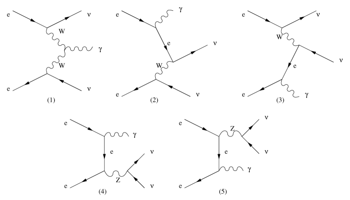
Figure 1: The Feynman diagrams for the $e^{-}e^{+}\to\nu\bar{\nu}\gamma$ process. Only the bottom two diagrams contribute to the $\nu_{\mu}\bar{\nu}_{\mu}\gamma$ and $\nu_{\tau}\bar{\nu}_{\tau}\gamma$ final states.

From the preceding discussions, and as is easily verified by explicit calculation, the $Z^{0}$ mediated contribution to the moment distribution is proportional to up to $\cos^{2}\!\theta$ only. It is not so obvious that this is still the case for the $W^{\pm}$ mediated contribution and the interference between the two contributions.

The analytical expression for this process, which includes both the $Z^{0}$ and $W^{\pm}$ contributions, is given in Eqns. (2)–(5) of Ref. [15]. There is an error in equation (3) available therein, and one should correct this error. The $s^{\prime}$ in the overall factor should only multiply the first two terms inside the square brackets. The expression without this correction is dimensionally inconsistent. We have performed four more independent calculations, out of which two are analytic and the other two use HELAS [16], and verified that the numbers are consistent with each other.

To motivate the discussion, let us first consider the $W^{\pm}$ mediated background in the limit of large $W^{\pm}$ mass. In this case the $W^{\pm}$ fusion graph (1) of Fig. 1 vanishes and we have only graphs (2) and (3), both of which can be written in terms of an effective contact interaction between two charged currents.

However, by Fierz transformation, this contact interaction between two charged currents is equivalent to the contact interaction between two neutral currents, and so the amplitude has identical form to the $Z^{0}$ mediated background [17]. Hence the distribution is only proportional to up to $\cos^{2}\!\theta$.

Furthermore, also by Fierz transformation, the SUSY signal $\widetilde{\gamma}\widetilde{\gamma}\gamma$, or more generally $\widetilde{\chi}^{0}_{1}\widetilde{\chi}^{0}_{1}\gamma$, has the same structure in the limit of large selectron mass. We thus obtain the expressions listed in Tabs. 1, 2.

It is found [18] that at LEP energies, although the above consideration of the heavy $W^{\pm}$ limit is clearly inappropriate, the shapes of angular distributions corresponding to the $Z^{\pm}$ and $W^{\pm}$ mediated contributions are fairly similar. There is no guarantee that this will still hold at future LC energies, and explicit evaluation indeed shows that there is nonvanishing $\cos 4\theta$ and higher contributions.

Even so, what becomes clear is the following. Let us consider the general case of the production of a photon and two invisible objects. If the particle exchanged in the $t$ channel is heavy, as is the case for the SUSY $\widetilde{\chi}^{0}_{1}\widetilde{\chi}^{0}_{1}\gamma$ production mediated by $t$-channel selectron exchange, the interaction is approximated by a contact interaction and then the distribution can only show a $\cos 2\theta$ behaviour. On the other hand, if the exchanged particle is light, as is the case for the $W^{\pm}$ contribution to the SM background at LC energies, the interaction is expected to be well understood and so the contribution can be subtracted, either from the bare distribution or from the Fourier coefficients. This provides partial justification for our procedure.

We also note that the $W^{\pm}$ mediated background involves left-handed electrons and right-handed positrons, and therefore it can be reduced by means of beam polarization.

2.4 Experimental Limitations

The experimental limitations which we take into account are the calorimeter resolution, angular coverage and beamstrahlung. The angular resolution is not expected to be a serious constraint. Beamstrahlung is treated using CIRCE [19] as discussed in the next Subsection.

For the EM calorimeter resolution, the EM track energy resolution $\Delta E$ is expected to be [20, 21]:

$$\frac{\Delta E}{E} = \frac{15\%}{\sqrt{E(\mathrm{GeV})}}\oplus 1\%\ ({\rm JLC})$$ (11)

$$= \frac{20\%}{\sqrt{E(\mathrm{GeV})}}\oplus 0.6\%\ ({\rm TESLA}).$$ (12)

This smears the photon energy distribution. As an example, for a 100 GeV photon, $\Delta E$ at JLC is 1.8 GeV, wheres at TESLA $\Delta E=2.1$ GeV. For photon energies lower than about 250 GeV, the energy resolution is always better at JLC. As a pessimistic estimate, although this choice does not affect our results in any visible way, let us adopt the TESLA numbers in our analysis.

Next, let us consider the coverage of the EM calorimeter. Typical numbers for this coverage [20, 21] are in the range 50 mrad–200 mrad. In this study, let us adopt $|\cos\theta|<0.995$, which corresponds to an angular cut-off of $\theta_{\rm min}=100$ mrad [20].

The derivation of the Fourier coefficients is completely successful only when the range of integration is propotional to the cyclic bound. The angular coverage is expected to become a problem if the Fourier component under consideration changes phase near this unmeasured region. For a Fourier component proportional to $\cos(2n\theta)$, the first change of phase occurs at $\theta=\pi/4n$. If we wish to measure $n\leq 3$, we need a coverage down to $\theta_{\rm min}<\pi/12=260$ mrad.

Explicit evaluation shows that the vanishing of the term $a_{3}\cos(6\theta)$ is indeed contaminated with the above coverage, $|\cos\theta|<\cos\theta_{\rm min}=0.995$. In order to evade this problem, as a simple remedy, we perform the extrapolation, that is, the approximation that the values in the non-coverage regions have constant values equal to the end-points. This is illustrated in Fig. 2.

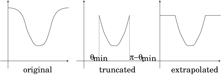
Figure 2: Illustrating the extrapolation procedure. The vertical axis is the $E_{T}^{2}$ moment distribution, and the horizontal axis is $\theta$. The $x_{\gamma}$ dependence is not shown.

The coefficient functions in Eqn. (8) and (9) are then redefined by

$$a_{0}(x_{\gamma}) = \frac{1}{2\pi}\Biggl{\{}\int_{2\theta_{\rm min}}^{2[\pi-\theta_{\rm min}]}\frac{E_{T}^{2}d^{2}\sigma}{d\cos\theta dx_{\gamma}}d(2\theta)$$

$$+ \int_{0}^{2\theta_{\rm min}}\left.\frac{E_{T}^{2}d^{2}\sigma}{d\cos\theta dx_{\gamma}}\right|_{\theta=\theta_{\rm min}}d(2\theta)+\int_{2[\pi-\theta_{\rm min}]}^{2\pi}\left.\frac{E_{T}^{2}d^{2}\sigma}{d\cos\theta dx_{\gamma}}\right|_{\theta=\pi-\theta_{\rm min}}d(2\theta)\Biggr{\}},$$

$$a_{m}(x_{\gamma}) = \frac{1}{\pi}\Biggl{\{}\int_{2\theta_{\rm min}}^{2[\pi-\theta_{\rm min}]}\frac{E_{T}^{2}d^{2}\sigma}{d\cos\theta dx_{\gamma}}\cos(2m\theta)d(2\theta)$$

$$+ \int_{0}^{2\theta_{\rm min}}\left.\frac{E_{T}^{2}d^{2}\sigma}{d\cos\theta dx_{\gamma}}\right|_{\theta=\theta_{\rm min}}\cos(2m\theta)d(2\theta)$$

$$+ \int_{2[\pi-\theta_{\rm min}]}^{2\pi}\left.\frac{E_{T}^{2}d^{2}\sigma}{d\cos\theta dx_{\gamma}}\right|_{\theta=\pi-\theta_{\rm min}}\cos(2m\theta)d(2\theta)\Biggr{\}}\qquad(m=1,2,3,\ldots).$$

We have found that this remedy is sufficient to overcome the problem at hand. We note that in the presence of ISR, the angles quoted above are measured in the laboratory frame rather than the centre-of-mass frame. This makes the imposition of the above cut-and-extrapolation procedure more difficult, and we adopt an approximate, ‘wrong’, solution which is to impose the angular cut and extrapolation in the centre-of-mass frame. Of course the evaluation of the integral is otherwise performed in the laboratory frame, as required.

For the centre-of-mass energy we mainly take $\sqrt{s}=500$ GeV. We also consider the $\sqrt{s}$ dependence by varying this to 1 TeV. We omit the discussion of statistics in this paper, but the luminosity may be considered to be in the region 100–500 fb^-1 per year [20, 21].

2.5 Initial State Radiation

The non-singular part of the higher order perturbative contributions is expected to mainly affect the normalization and not the shape of the distributions. However, the logarithmically enhanced bremsstrahlung corrections must be considered for realistic simulation. There is another source of ISR, that is, beamstrahlung. We consider both effects.

Beamstrahlung is the radiation of photon caused by the interaction between the incoming electron and positron bunches. This smears both the centre-of-mass energy and the momentum along the beam axis. We use CIRCE [19] in order to estimate this effect.

Bremsstrahlung is the radiation caused by the interaction between the electron and the positron participating in the annihilation event. We estimate this effect by using the integrated expression of [22]. This does not take into account the effect of large angle emission into the detector, nor does it take into account the emission of more than one photon from each incoming particle, but is expected to model the dominant effect well.

As an illustration, the typical energy carried by a bremsstrahlung photon is

$$\int_{0}^{1}d(E,x)\ (Ex)\ dx,$$ (15)

where, from the expression of [22],

$$d(E,x)\sim\frac{\alpha_{EM}}{\pi}\frac{2}{x}(\log\frac{E}{m_{e}}-\frac{1}{2})\sim\frac{0.063}{x}\ (E\sim 250\!\mathrm{GeV}).$$ (16)

Hence Eqn. (15) yields 16 GeV for a 250 GeV beam. This energy taken away by the photon affects both the centre-of-mass energy and the frame. This change of frame implies a Lorentz boost to the final state photon and so the angular distribution is also affected, as well as the energy distribution.

The subdominant ‘hard bremsstrahlung’, where photons enter into the detectable region, is not treated in this paper, but we expect that a minimum $E_{T}$ cut is necessary to reduce such effect. Such a cut would also be effective in reducing the background coming from low $E_{T}$ Bhabha and forward photon events. This would be equivalent to assigning an energy dependent cut for the minimum polar angle $\theta_{\rm min}$, and we expect that this can be dealt with by the extrapolation procedure adopted for calorimeter coverage in the preceding Subsection. As an example, for a 50 GeV photon, requiring $E_{T}>10$ GeV corresponds to $\theta_{\rm min}=201$ mrad. Further study is desirable to quantify this effect.

As an illustrative example, we consider a configuration in which a photon is produced at $x_{\gamma\rm CM}=1,\cos\theta_{\rm CM}=0$. The Lorentz boost is easily shown to be given in terms of the electron and positron momentum fractions $x_{1}$ and $x_{2}$ by:

$$\cos\theta_{\rm lab} = \frac{x_{1}-x_{2}}{x_{1}+x_{2}},$$ (17)

$$x_{\gamma\rm lab} = \frac{x_{1}+x_{2}}{2}.$$ (18)

The effective centre-of-mass energy is given by $\sqrt{\hat{s}}=\sqrt{sx_{1}x_{2}}$. One can immediately verify that the transverse energy is unaffected by this boost and is given by $E_{T}=\sqrt{\hat{s}}/2$. We can now plot these functions for a given centre-of-mass energy $\sqrt{s}$ and beamstrahlung spectrum. Taking $\sqrt{s}=500$ GeV and the TESLA beamstrahlung spectrum, we obtain the results shown in Fig. 3.

Figure 3: Distributions of $\cos\theta$ (left) and $x_{\gamma}$ (right) of the $x_{\gamma\rm CM}=1,\cos\theta_{\rm CM}=0$ events after beamstrahlung and bremsstrahlung. The distributions are normalized to unity.

From these figures, we can obtain a rough estimate of the effect of ISR. $\cos\theta$, or equivalently $\theta$, is smeared typically by about 0.01 (radians). Although this smearing is small enough for us to expect that ISR will not change the angular distribution so much as to produce non-vanishing higher Fourier components, there is a relatively long tail to the distribution which may yield non-negligible effect.

For small smearing, $x_{1},x_{2}\sim 1$, the polar angle dependence of the angular smearing can be shown to go as:

$$\delta\theta_{\rm lab}\approx\frac{x_{1}-x_{2}}{2}\sin\theta.$$ (19)

As expected, the angular smearing is the largest when $\theta=\pi/2$.

The energy fraction is smeared by about 0.01, which is comparable to the calorimeter resolution. This is again accompanied by a long tail. As the cross section is proportional to $(\sqrt{s})^{n}$, we expect that this suppression in the effective centre-of-mass energy may lead to a significant suppression of the cross section.

3 Results

In this Section, we follow our analysis numerically. The parameters related to the graviton emission, the fundamental scale and the number of extra dimensions, are taken to be $M_{D}=1$ TeV and $n=2$ for now.

In Fig. 4, the $\cos\theta$ dependence for the process $e^{+}e^{-}\rightarrow G\gamma$ at $\sqrt{s}=500$ GeV is shown, together with the corresponding plot for on-shell $Z^{0}$ production. A cut on the energy fraction of the photon is taken as $x_{\gamma}>0.05$. In the plot for on-shell $Z^{0}$ production, we also show the distribution for the production of a hypothetical scalar $Z^{0}$. The normalization is arbitrary in this case. For this set of parameters, we see that the total rates are quite similar.

Figure 4: The subprocess level $\cos\theta$ distribution, for the graviton events integrated over $0.05<x_{\gamma}<1$ (left), and the on-shell $Z^{0}\to\nu\bar{\nu}$ events (right). For the $Z^{0}$ events, we also show the hypothetical production of a spin-0 object of the same mass (lower curve). The normalization is arbitrary in this case.

From Fig. 4, we see that at first sight, there is no clear distinction between the distributions due to the production of objects of different spin. We therefore look mainly at the $E_{T}^{2}$ moment distribution, as explained in the preceding Sections.

We then apply the Fourier expansion to this moment distribution, as expressed in Eqns. (8) and (9). As mentioned before, this is not the only method to extract the Fourier coefficients, and it may turn out that a $\chi^{2}$ based fit is more practical. We take this approach because it is the most theoretically elegant, and also because it provides a convenient way of parameterizing the two dimensional distribution of $x_{\gamma}$ and $\cos\theta$.

Fig. 5 shows the Fourier coefficients for graviton events, before applying any corrections, as functions of the energy fraction $x_{\gamma}$. We see that only the first three coefficient functions are non-zero, as expected.

Figure 5: The Fourier coefficients in units of fb GeV² for graviton events, before applying any corrections.

When we truncate the distribution to account for the finite coverage of the calorimeter as stated in Sect. 2.4, $a_{m}$ for large $m$ acquires an artefactual contribution and becomes non-zero. However, we recover the original distribution by the extrapolation procedure proposed above. The situation is illustrated in Fig. 6.

Figure 6: The Fourier coefficients for graviton events, after including the calorimeter coverage (left), and after the correction by extrapolation (right).

As the corrected distribution shown in Fig. 6 looks almost identical to the original distribution shown in Fig. 5, we conclude that the procedure is sufficient for our purpose.

Let us now take into account the effects of bremsstrahlung and beamstrahlung and, perhaps less importantly, the calorimeter energy resolution. For the beamstrahlung and calorimeter energy resolution, although the choice is arbitrary and leads to little difference in the result, let us adopt the TESLA parameters.

The effect of the ISR is explained and illustrated in Sect. 2.5. Applying the same ISR spectrum to the signal, we obtain the results shown in Fig. 7. We see that the coefficients have dropped significantly, and there is further suppression as $x_{\gamma}\to 1$. This is as expected. The coefficient $a_{3}$ remains zero even with the inclusion of ISR.

Figure 7: The Fourier coefficients for graviton events, including all corrections.

Let us now turn our attention to the SM continuum background. The distribution is shown in Fig. 8. Again, the rate is quite similar to the signal for this set of extra dimensional parameters. The dominant part of the background distribution for $x_{\gamma}<0.8$ is due to the $W^{\pm}$ mediated contribution. The rise of the cross section near $x_{\gamma}=1$ is due to the $Z^{0}$. The coefficients $a_{2}$ and $a_{3}$ do not have a peak for this reason. However, there is the interference term between the $Z^{0}$ and $W^{\pm}$ mediated contributions, and this interference term gives rise to the observed behaviour near $x_{\gamma}=0.95$. With the inclusion of ISR, the $Z^{0}$ peak broadens. At the same time, the angular smearing due to the ISR gives rise to additional contributions to $a_{2}$ and $a_{3}$ at the $Z^{0}$ peak, which lead to the interesting behaviour observed near that region.

From these figures, it is clear that the proper simulation of the ISR is essential to understanding both the signal and the background.

Figure 8: The Fourier coefficients for the SM continuum background, without the experimental and bremsstrahlung corrections (left), and including all corrections (right).

As noted in Sect. 2.3, $a_{2}$ and higher coefficients are in general non-zero for $\sqrt{s}$ sufficiently higher than $M_{W}$. The explicit evaluation, as shown in Fig. 8, confirms this. Although these coefficients are non-zero, we note, again, that the shape of the background is sufficiently well understood that the distribution can be subtracted away, either from the bare distribution or the Fourier coefficients.

Finally, let us turn our attention to the centre-of-mass energy, $\sqrt{s}$, dependence of the distributions, and the dependence of the signal distribution on the number of extra dimensions $n$.

In order to understand the centre-of-mass energy dependence, we calculated the signal and background Fourier coefficients, which have so far been calculated for $\sqrt{s}=500$ GeV, for $\sqrt{s}=1$ TeV, including all corrections. The result is shown in Fig. 9.

Figure 9: The signal (left) and background (right) Fourier coefficients, at $\sqrt{s}=1$ TeV, including all corrections.

We see that there is a significant change in the shape of the background distribution when the centre-of-mass energy is raised. The signal distribution does not change much, but if there is any difference, it is expected to be due to the increased beamstrahlung. The total rate is increased for the signal and reduced for the background. For the case of the background, although the cross section is reduced, the size of the $E_{T}^{2}$ moment distribution is increased because of the centre-of-mass energy dependence of the total effective $e^{-}e^{+}$ charged current cross section which, in the limit of large energy, becomes flat.

In order to understand the dependence on the number of extra dimensions $n$, we calculated the signal Fourier coefficients for $n=4$ and $n=7$, at $\sqrt{s}=500$ GeV, again including all corrections. The result is shown in Fig. 10.

Figure 10: The signal Fourier coefficients for $n=4$ (left) and $n=7$ (right).

We see that as $n$ becomes larger, the Fourier coefficients are more suppressed towards larger $x_{\gamma}$ because of the factor $(1-x_{\gamma})^{n/2-1}$. The higher Fourier coefficients, which rise with $x_{\gamma}$ as powers of $x_{\gamma}$, become suppressed, and the $E_{T}^{2}$ moment distribution becomes more flat. In this limit, it becomes impossible to determine the spin from the angular distribution only, and one would have to resort to the $\chi^{2}$ fitting, for example, of the leading Fourier coefficient $a_{0}$ as a function of $x_{\gamma}$ in order to discriminate the extra dimensional hypothesis from other hypotheses. This method would also be useful when there is not sufficient statistics to utilize the angular distribution.

It may be argued that the presence of a quartic polynomial in the coefficient $a_{0}$, as shown in Tab. 2 indicates the spin-2 nature. This is less rigourous, and there would remain the possibility that the shape is due to the distribution of gravitons. We also note that the size of the quartic term is not large.

To some extent the difference in the shape of the Fourier coefficients can be exploited to ‘measure’ the number of extra dimensions, or more precisely the distribution of the Kaluza-Klein modes. One can alternatively measure the $\sqrt{s}$ dependence of these coefficients, proportional to $\sqrt{s}^{n+2}$ for $n$ extra dimensions, to yield the same information.

Having outlined the application of our procedure thus, one may like to question the statistical efficacy of our observables. Although a formal discussion would require a more detailed study, it is a simple matter to have a rough estimation of the statistics. If we assume a relatively low integrated luminosity $\mathcal{L}=100$ fb^-1, and look, for instance, at the numbers at 500 GeV shown in Fig. 7, and take $0.8<x_{\gamma}<0.9$, say, a quick estimation of the numbers show that the significance defined as ‘$S/\sqrt{B}$’$=\sqrt{\mathcal{L}\Delta x_{\gamma}a_{2}^{2}/(E_{T}^{2}a_{0})}\sim 2$ so that 95% confidence level can be attained even with low luminosity for this set of $n$ and $M_{D}$.

4 Conclusions

We have proposed a way of measuring the ‘spin’ of invisible objects, including gravitons, produced at future LC.

Our method is to measure the Fourier coefficients $a_{m}(x_{\gamma})$ ($m=0,1,2\cdots$) of the $E_{T}^{2}$ moment distributions. The presence of terms up to $a_{S}$ and the absence of the higher coefficients indicates the spin-$S$ nature of the invisible object.

We have provided a theoretical justification for this observation, and have carried out a simulation based on this principle. Our simulation includes the consideration of beamstrahlung, bremsstrahlung, calorimeter coverage, calorimeter resolution and the background, and we believe that the simulation is realistic. The ISR, composed of beamstrahlung and bremsstrahlung, has a particularly marked effect on both the signal and the background. Our study is nevertheless incomplete, as the statistical study and the error estimation have not been performed. When doing so, it is desirable that further attention is paid to the effect of the hard/multiple bremsstrahlung contribution which must be dealt with more carefully.

This method as stated is useful when the number of extra dimensions $n$ is 2. If we believe in the astrophysical constraint, this case may be ruled out. For greater $n$, the direct application of this procedure is not suitable because the higher Fourier coefficients become small. Even in that case, the method provides a parameterization of the cross section which separates the angular and energy dependence. The resulting $x_{\gamma}$ dependent coefficient $a_{0}$, for example, can be subjected to $\chi^{2}$ analysis in order to test the extra dimensional hypothesis.

We also note that the shape of the Fourier coefficient functions will provide a measure of the ‘number’ of extra dimensions. More generally, the measurement of spin aside, what our method provides is a framework by which we may parameterize single photon events at future LC.

References

-
[1]
N. Arkani-Hamed, S. Dimopoulos and G. R. Dvali,
Phys. Lett. B 429, 263 (1998)
[arXiv:hep-ph/9803315];
I. Antoniadis, N. Arkani-Hamed, S. Dimopoulos and G. R. Dvali, Phys. Lett. B 436, 257 (1998) [arXiv:hep-ph/9804398]. - [2] B. Abbott et al. [D0 Collaboration], Phys. Rev. Lett. 86, 1156 (2001) [arXiv:hep-ex/0008065].
- [3] M. Acciarri et al. [L3 Collaboration], Phys. Lett. B 464, 135 (1999) [arXiv:hep-ex/9909019]. M. Acciarri et al. [L3 Collaboration], Phys. Lett. B 470, 281 (1999) [arXiv:hep-ex/9910056].
- [4] S. Cullen and M. Perelstein, Phys. Rev. Lett. 83, 268 (1999) [arXiv:hep-ph/9903422]. S. Hannestad and G. Raffelt, Phys. Rev. Lett. 87, 051301 (2001) [arXiv:hep-ph/0103201]. C. Hanhart, J. A. Pons, D. R. Phillips and S. Reddy, Phys. Lett. B 509, 1 (2001) [arXiv:astro-ph/0102063].
- [5] L. J. Hall and D. R. Smith, Phys. Rev. D 60, 085008 (1999) [arXiv:hep-ph/9904267].
- [6] G. F. Giudice, R. Rattazzi and J. D. Wells, Nucl. Phys. B 544, 3 (1999) [arXiv:hep-ph/9811291].
- [7] T. Han, J. D. Lykken and R. J. Zhang, Phys. Rev. D 59 105006 (1999) [arXiv:hep-ph/9811350].
- [8] E. A. Mirabelli, M. Perelstein and M. E. Peskin, Phys. Rev. Lett. 82, 2236 (1999) [arXiv:hep-ph/9811337]. K. Cheung, Phys. Rev. D 61, 015005 (2000) [arXiv:hep-ph/9904266].
- [9] K. Cheung and W. Y. Keung, Phys. Rev. D 60, 112003 (1999) [arXiv:hep-ph/9903294]. K. Agashe and N. G. Deshpande, Phys. Lett. B 456, 60 (1999) [arXiv:hep-ph/9902263]. K. Y. Lee, H. S. Song and J. Song, Phys. Lett. B 464, 82 (1999) [arXiv:hep-ph/9904355]. O. J. Eboli, M. B. Magro, P. Mathews and P. G. Mercadante, Phys. Rev. D 64, 035005 (2001) [arXiv:hep-ph/0103053]. K. Cheung, arXiv:hep-ph/0104250. T. G. Rizzo, arXiv:hep-ph/0108235.
- [10] S. Gopalakrishna, M. Perelstein and J. D. Wells, arXiv:hep-ph/0110339.
- [11] P. Mathews, S. Raychaudhuri and K. Sridhar, JHEP 0007, 008 (2000) [arXiv:hep-ph/9904232]. T. Han, D. Rainwater and D. Zeppenfeld, Phys. Lett. B 463, 93 (1999) [arXiv:hep-ph/9905423]. O. J. Eboli, T. Han, M. B. Magro and P. G. Mercadante, Phys. Rev. D 61, 094007 (2000) [arXiv:hep-ph/9908358]. K. Cheung and G. Landsberg, Phys. Rev. D 62, 076003 (2000) [arXiv:hep-ph/9909218]. D. Atwood, S. Bar-Shalom and A. Soni, Phys. Rev. D 62, 056008 (2000) [arXiv:hep-ph/9911231]. B. C. Allanach, K. Odagiri, M. A. Parker and B. R. Webber, JHEP 0009, 019 (2000) [arXiv:hep-ph/0006114]. M. A. Doncheski, arXiv:hep-ph/0111149.
- [12] P. Mathews, P. Poulose and K. Sridhar, Phys. Lett. B 461, 196 (1999) [arXiv:hep-ph/9905395]. T. G. Rizzo, Phys. Rev. D 60, 115010 (1999) [arXiv:hep-ph/9904380]. H. Davoudiasl, Phys. Rev. D 60, 084022 (1999) [arXiv:hep-ph/9904425]. D. K. Ghosh, P. Mathews, P. Poulose and K. Sridhar, JHEP 9911, 004 (1999) [arXiv:hep-ph/9909567]. M. A. Doncheski and R. W. Robinett, Phys. Rev. D 61, 117701 (2000) [arXiv:hep-ph/9910346]. K. Y. Lee, S. C. Park, H. S. Song, J. Song and C. Yu, Phys. Rev. D 61, 074005 (2000) [arXiv:hep-ph/9910466]. T. G. Rizzo, Nucl. Instrum. Meth. A 472, 37 (2001) [arXiv:hep-ph/0008037].
- [13] D. K. Ghosh, P. Poulose and K. Sridhar, Mod. Phys. Lett. A 15, 475 (2000) [arXiv:hep-ph/9909377]. D. Atwood, S. Bar-Shalom and A. Soni, Phys. Rev. D 61, 116011 (2000) [arXiv:hep-ph/9909392].
- [14] S. B. Giddings and S. Thomas, arXiv:hep-ph/0106219. S. Dimopoulos and G. Landsberg, Phys. Rev. Lett. 87, 161602 (2001) [arXiv:hep-ph/0106295]. M. B. Voloshin, Phys. Lett. B 518, 137 (2001) [arXiv:hep-ph/0107119]. S. Dimopoulos and R. Emparan, Phys. Lett. B 526, 393 (2002) [arXiv:hep-ph/0108060]. K. Cheung, arXiv:hep-ph/0110163. R. Casadio and B. Harms, arXiv:hep-th/0110255. A. Ringwald and H. Tu, Phys. Lett. B 525, 135 (2002) [arXiv:hep-ph/0111042]. S. Hofmann, M. Bleicher, L. Gerland, S. Hossenfelder, S. Schwabe and H. Stocker, arXiv:hep-ph/0111052. S. C. Park and H. S. Song, arXiv:hep-ph/0111069. M. B. Voloshin, Phys. Lett. B 524, 376 (2002) [arXiv:hep-ph/0111099]. T. G. Rizzo, arXiv:hep-ph/0111230. K. y. Oda and N. Okada, arXiv:hep-ph/0111298. G. Landsberg, arXiv:hep-ph/0112061. G. F. Giudice, R. Rattazzi and J. D. Wells, arXiv:hep-ph/0112161. M. Bleicher, S. Hofmann, S. Hossenfelder and H. Stocker, arXiv:hep-ph/0112186. E. J. Ahn, M. Cavaglia and A. V. Olinto, arXiv:hep-th/0201042. D. M. Eardley and S. B. Giddings, arXiv:gr-qc/0201034. T. G. Rizzo, arXiv:hep-ph/0201228. S. N. Solodukhin, arXiv:hep-ph/0201248.
- [15] F. A. Berends, G. J. Burgers, C. Mana, M. Martinez and W. L. van Neerven, Nucl. Phys. B 301, 583 (1988).
- [16] H. Murayama, I. Watanabe and K. Hagiwara, KEK-91-11.
- [17] K. J. Gaemers, R. Gastmans and F. M. Renard, Phys. Rev. D 19, 1605 (1979). M. Caffo, R. Gatto and E. Remiddi, Phys. Lett. B 173, 91 (1986); Nucl. Phys. B 286, 293 (1987).
- [18] G. Montagna, M. Moretti, O. Nicrosini and F. Piccinini, Nucl. Phys. B 541, 31 (1999).
- [19] T. Ohl, Comput. Phys. Commun. 101, 269 (1997) [arXiv:hep-ph/9607454].
- [20] J. A. Aguilar-Saavedra et al. [ECFA/DESY LC Physics Working Group Collaboration], arXiv:hep-ph/0106315.
- [21] K. Abe et al. [ACFA Linear Collider Working Group Collaboration], arXiv: hep-ph/0109166.
- [22] B. Grzadkowski, S. Pokorski and J. Rosiek, Phys. Lett. B 272, 143 (1991).