We construct a parametrization of deep–inelastic structure functions which retains information on experimental errors and correlations, and which does not introduce any theoretical bias while interpolating between existing data points. We generate a Monte Carlo sample of pseudo–data configurations and we train an ensemble of neural networks on them. This effectively provides us with a probability measure in the space of structure functions, within the whole kinematic region where data are available. This measure can then be used to determine the value of the structure function, its error, point–to–point correlations and generally the value and uncertainty of any function of the structure function itself. We apply this technique to the determination of the structure function $F_{2}$ of the proton and deuteron, and a precision determination of the isotriplet combination $F_{2}$[p-d]. We discuss in detail these results, check their stability and accuracy, and make them available in various formats for applications.

April 2002

1 Determining Structure Functions

Recently, a considerable amount of theoretical and experimental effort has been invested in the accurate determination of the parton distributions of the nucleon, and in particular their associate errors, in view of the accurate computation of collider processes and determination of QCD parameters [1]–[5]. The determination of parton distributions requires unfolding the experimentally measurable structure functions in terms of their parton content, by resolution of the QCD evolution equations. However, for many applications, it is desirable and sufficient to deal directly with the experimentally measurable structure functions themselves. For instance, the nonsinglet structure function $F_{2}$ coincides with the (DIS–scheme) quark distribution, and thus in particular the strong coupling can be extracted directly from its scaling violations [6]. Also, knowledge of the structure function $F_{2}$ is needed for data analysis: for instance, when extracting polarized structure functions from cross–section asymmetries [7].

For all these applications, one needs to know the structure function $F_{2}$ as a function of $x$ and $Q^{2}$, and not only for the particular values where it has been measured. Therefore, even though the laborious task of disentangling the parton content of the target and solving the evolution equations is not necessary if one directly determines the structure function, the central problem is the same as in the determination of parton distributions. Namely, one has to determine a function, and associate error, from a finite set of measurements. Because a function is an infinite–dimensional object, this is an a priori ill–posed problem, unless one makes some extra assumptions. The simplest way of implementing suitable extra assumption is to assume that the given function has a certain functional form, parametrized by a finite number of parameters, which can then be fitted from the data. However, the choice of a specific functional form is in general quite restrictive: therefore, it is thus a source of bias, i.e. systematic error which is very difficult to control. Furthermore, when fitting a fixed functional form to the data, it is very hard to obtain a determination not only of the best-fit parameters, but also of their errors (and correlations): systematic uncertainties are difficult to take into account [2, 5], and conventional error propagation and determination of the covariance matrix in a fixed parameter space is unwieldy and may fail because of linearization problems.

A way out of these difficulties, based on the direct determination of the measure in the space of parton distributions by Monte Carlo sampling has been proposed [3, 4]. However, it is computationally quite intensive, and it has not yet led to a full set of parton distributions with errors. Here, we propose a new approach to the determination of structure functions which also aims at the determination of the measure in the space of structure functions. Our approach is based on the use of neural networks as basic interpolating tools. The peculiar feature of neural networks which we will exploit is that they can provide an interpolation without requiring any assumption (other than continuity) on the functional form of the underlying law fulfilled by the given observable. Hence, given a sampling of the measure in the space of function over a finite set of points, the neural networks can provide an unbiased interpolation which gives us the measure for all points, at least within a range of $x$ and $Q^{2}$ where the sampling provided by the data is fine enough.

We will use this procedure to construct parametrizations of the structure function $F_{2}$ for the proton, the deuteron, and an independent precision determination of the nonsinglet combination $F_{2}^{p}-F_{2}^{d}$. We will analyze in detail the properties of our results, and show that they reproduce correctly the information contained in the data, while interpolating smoothly between data points. We will also see that when the separation of data points in $x$ and $Q^{2}$ is smaller than a certain correlation length, the neural net manages to combine the corresponding experimental information, thus leading to a determination of the structure function which is more accurate than that of individual experiments, and we will devise statistical tests to ascertain that this is achieved in an unbiased way.

In Sect. 2 we will introduce the problem of constructing a parametrization of structure functions, the data that we will use, discuss previous solutions of this problem, and motivate our alternative approach. In Sect. 3 we will then provide some general background on neural networks, and in Sect. 4 we will describe our method for the construction of a neural parametrization of structure functions. Finally, in Sect. 5 we will turn to a discussion and assessment of our results. First we will discuss the theoretically simpler nonsinglet structure function: we will examine the compatibility of different experiments, and the ability of the neural networks to combine different pieces of experimental information. Then, we will tackle the determination of the individual proton and deuteron structure functions, and discuss the accuracy of our results.

2 Parametrization of Structure functions

Our aim in this paper is to construct a simultaneous parametrization of the structure functions $F_{2}$ for the proton and deuteron: we start from a set of measurements of a structure function, say $F_{2}$, for a discrete set of values of $x$ and $Q^{2}$, and we wish to determine $F_{2}(x,Q^{2})$ as a function defined in a certain range of $x$ and $Q^{2}$. We choose the structure function $F_{2}$ as determined in neutral–current DIS of charged leptons, since an especially wide set of experimental determinations of it is available, and also because it is of direct theoretical interest. Studies of charged–current, neutrino, and polarized structure functions will be left to future work.

A simultaneous determination of the structure functions for proton and deuteron is very useful for applications, since it amounts to a simultaneous determination of the isospin singlet and triplet components of the structure function. Also, such a simultaneous determination poses peculiar theoretical problems, given that we aim at a determination of the full set of correlations.

In fact, we will provide both a determination of the correlated pair of proton and deuteron structure functions, as well as a separate determination of the isotriplet component. This is both useful and interesting because, as we shall see, data on the isotriplet combination turn out to be affected by much larger percentage errors, i.e. to have a much less favourable signal–to–noise ratio: the isotriplet is generally a small number obtained as the difference of two numbers which are by an order of magnitude larger. Therefore, on the one hand a more precise determination can be obtained by a dedicated analysis, rather than just taking a difference, on the other hand this determination will turn out to have peculiar features which deserve a specific study.

Parametrizations of structure functions have been constructed before, and used for the applications discussed in the introduction. In this section, we will first describe the specific data set that we will use, and then briefly review existing approaches to the parametrization of structure functions and their shortcomings.

2.1 Experimental data

We will use the data of the New Muon Collaboration (NMC) [8] and the BCDMS (Bologna-CERN-Dubna-Munich-Saclay) Collaboration [9] on the structure function $F_{2}$ of proton and deuteron. These data provide a simultaneous determination of the proton and deuteron structure functions in the same kinematic region, and provide the full set of correlated experimental systematics for these measurements. Earlier data from SLAC are not competitive with these in terms of accuracy and kinematic coverage. The more recent HERA data are available in a much wider kinematic region, but only for proton targets. Another set of joint proton and deuteron measurements was performed by the E665 Collaboration [10]. These data are mostly concentrated at low $Q^{2}$ (and low $x$): 80% of the data have $Q^{2}<1$ GeV². They are therefore somewhat less interesting for perturbative QCD applications, and we will leave them out of the present analysis. We have checked that their inclusion would have a negligible impact on the determination of the structure function in the region covered by NMC and BCDMS. The kinematic coverage of the data which we include in our analysis is displayed in Figure 1. A better coverage of the large $x$ region at moderate $Q^{2}$ might be achievable in the near future by combining some of the earlier SLAC data [11] with forthcoming JLAB data [12].

2.1.1 NMC

The NMC data consist of four data sets for the proton and the deuteron structure functions corresponding to beam energies of $90$ GeV ($72$ p and $72$ d data points), 120 GeV ($64+64$ data points), $200$ GeV ($74+74$ data points), and $280$ GeV ($78+78$ data points). They cover the kinematic range $0.002\leq x\leq 0.60$ and $0.5\,\rm{GeV}^{2}\leq Q^{2}\leq 75\,\rm{GeV}^{2}$. The systematic errors, given in Ref.  [8], are:

• uncertainty on the incoming and outgoing beam energies, fully correlated between proton and deuteron data, but independent for data taken at different beam energies ($E$, $E^{\prime}$);

• radiative corrections, fully correlated between all energies, but independent for proton and deuteron ($RC$);

• acceptance ($AC$) and reconstruction efficiency ($RE$) , fully correlated for all data sets;

• normalization uncertainty, correlated between the proton and the deuteron data, but independent for data taken at different beam energies ($\sigma_{N}$).

In this experiment, correlation between proton and deuteron data are due to the fact that both targets were exposed to the beam simultaneously.

The uncertainties due to acceptance range from 0.1 to 2.5% and reach at most 5% at large $x$ and $Q^{2}$. The uncertainty due to radiative corrections is highest at small $x$ and large $Q^{2}$ and is at most 2%. The uncertainty due to reconstruction efficiency is estimated to be 4% at most. The uncertainties due to the incoming and the scattered muon energies contribute to the systematic error by at most 2.5%. The normalization uncertainty is 2%.

Figure 1: NMC and BCDMS kinematic range.

2.1.2 BCDMS

The BCDMS data consist of four data sets for the proton structure function, corresponding to beam energies of $100$ GeV (97 data points), $120$ GeV (99 data points), $200$ GeV (79 data points) and $280$ GeV (76 data points), and three data sets for the deuteron structure function corresponding to beam energies of $120$ GeV (99 data points), $200$ GeV (79 data points) and $280$ GeV (76 data points). They cover the kinematic range $0.06\leq x\leq 0.80$ and $7\,\rm{GeV}^{2}\leq Q^{2}\leq 280\,\rm{GeV}^{2}$.

The systematic errors are: 

• calibration of the incoming muon (beam) energy ($f_{b}$);

• calibration of the outgoing muon energy (spectrometer magnetic field) ($f_{s}$);

• spectrometer resolution ($f_{r}$);

• absolute normalization uncertainty ($\sigma_{N_{a}}$);

• relative normalization uncertainties ($\sigma_{N_{t}}$, $\sigma_{N_{b}}$).

All these sources of systematics are fully correlated for all targets and for all beam energies, despite the fact that measurements with different targets were done at different times, for the following reasons [13]: the calibration of the incoming beam energy E was dominated by a systematic uncertainty which was more stable in time than the precision of measurements; the calibration of the outgoing muon energy was reproducible to high relative accuracy throughout the experiment, independent of the target or beam energy; the resolution of the spectrometer depended on the constituent material, which did not change during the running of the experiment.

The uncertainty due to beam energy is smaller than 5 %, and those due to magnetic field and outgoing muon energy are smaller than 10 %; all uncertainties are most relevant at large $x$ and small $Q^{2}$. The absolute cross–section normalization error is 3%; relative normalization errors are $2\%$ between data taken with different targets, $1\%$ between data taken at different beam energies for the proton, $1\%$ between data taken at 120 GeV and 200 GeV and $1.5\%$ between data taken at 200 GeV and 280 GeV for the deuteron.

2.1.3 Correlation and covariance matrices

The structure of the correlation matrix, expressed in terms of the sources of systematics discussed above is as follows. For NMC

$$\rho_{ij} = {{F_{i}F_{j}}\over{\sigma_{i,tot}\sigma_{j,tot}}}$$ (1)

$$\times \left(E_{i}\,E_{j}+E^{\prime}_{i}\,E^{\prime}_{j}+AC_{i}\,AC_{j}+RC_{i}\,RC_{j}+RE_{i}\,RE_{j}+\sigma_{N}^{2}\right)$$

where $\sigma_{tot}=\sqrt{{\sigma_{s}}^{2}+F(\sigma_{c}^{2}+\sigma_{N}^{2})}$; $\sigma_{s}$ is the statistical error, $\sigma_{c}$ is the combination of correlated systematic errors, $\sigma_{N}$ is the normalization error, and systematic and normalization errors are given in percentage.

For BCDMS

$$\rho_{ij}={{F_{i}F_{j}}\over{\sigma_{i,tot}\sigma_{j,tot}}}\left(f_{b,i}\,f_{b,j}+f_{s,i}\,f_{s,j}+f_{r,i}\,f_{r,j}+\sigma_{N}^{2}\right)$$ (2)

with $\sigma_{N}=\sqrt{\sigma_{N_{a}}^{2}+\sigma_{N_{t}}^{2}+\sigma_{N_{b}}^{2}}$, where $\sigma_{N_{a}}$ is a global normalization error, $\sigma_{N_{t}}$ is the relative normalization between different targets and $\sigma_{N_{b}}$ is the relative normalization between different beam energies.

The covariance matrix is defined as

$$\mathrm{cov}_{ij}=\rho_{ij}\sigma_{i}\sigma_{j}.$$ (3)

In the sequel, we will also be interested in the covariance matrix of data for the nonsinglet structure function $F^{NS}\equiv F^{p}-F^{d}$. In general the covariance of two functions of $x_{i}$, $x_{j}$ is related to the covariance of these variables by

$$\mathrm{cov}(f(\vec{x}),g(\vec{x}))=\sum_{i,j}{{\partial f}\over{\partial x_{i}}}{{\partial g}\over{\partial x_{j}}}\mathrm{cov}(x_{i},x_{j})\ .$$ (4)

For the nonsinglet structure function we get

$$\mathrm{cov}(F^{p}_{i}-F^{d}_{i},F^{p}_{j}-F^{d}_{j})=\mathrm{cov}(F^{p}_{i},F^{p}_{j})+\mathrm{cov}(F^{d}_{i},F^{d}_{j})-\mathrm{cov}(F^{p}_{i},F^{d}_{j})-\mathrm{cov}(F^{d}_{i},F^{p}_{j})\ .$$ (5)

2.2 Structure function fits

Several structure function fits have been presented in the literature  [7, 10, 14]. They are all based on the idea of assuming a more or less simple functional from for the structure function $F_{2}$ (say), and then fitting its parameters. Once the free parameters of a given functional form are determined by fitting to the data, one can compute any function of $F_{2}$, such as e.g. its Mellin moments. In principle, given the error matrix of the parameters of the fit, one can also determine errors on $F_{2}$ and functions thereof by error propagation. Clearly, however, this is both impractical and subject to errors which are difficult to assess, because of the numerous linearizations which may be needed in order to determine the error on a physical observable (such as a Mellin moment) and, more importantly, because of the bias which is imposed by the choice of a specific functional form.

In order to overcome at least the practical difficulty of determining errors by propagation from the covariance matrix, a frequently adopted shortcut consists of giving a band of acceptable results, i.e. a pair of ‘upper’ and ‘lower’ values of the structure function, for each $(x,\,Q^{2})$. This error band can be again calculated either by means of the covariance matrix itself [7, 14], or by some other recipe which involves assessing the compatibility of a certain result with the data [5]. Whereas this may be sufficient in order to estimate the size of the error related to uncertainties on structure functions, it is clearly inadequate for a quantitative analysis, since there is no way to use these error bands to uniquely determine the error on a given quantity which depends on the structure function. For example, suppose one wants to determine the error on the integral over $x$ of the structure function: one might be tempted to identify this error with the spread of values of the integral computed from the upper and lower curves. This is however not correct, because it neglects the correlation between the structure function at different values of $x$, and it can in fact lead to a substantial overestimate of the error.

These difficulties can be traced to the fact that when fitting a structure function one is trying to determine a function, i.e. an infinite–dimensional quantity, from a finite set of measurements [3]. Assuming a functional form of the function projects the problem onto the finite–dimensional subspace of functions of the given form, but at the cost of introducing a bias when choosing how to perform this projection. A full, unbiased solution of the problem requires instead the determination of the probability measure ${\cal P}[F_{2}]$ in the space of functions $F_{2}(x,Q^{2})$, such that the expectation value of any observable ${\cal F}\left[F_{2}(x,Q^{2})\right]$ which depends on $F_{2}$ can be found by averaging with this measure:

$$\Big{\langle}{\cal F}\left[F_{2}(x,Q^{2})\right]\Big{\rangle}=\int\!{\cal D}F_{2}\,{\cal F}\left[F_{2}(x,Q^{2})\right]\,{\cal P}[F_{2}],$$ (6)

where the integral is a functional integral over the space of functions $F_{2}$ [3]. For example, ${\cal F}\left[F_{2}(x,Q^{2})\right]$ could be a Mellin moment of $F_{2}(x,Q^{2})$.

A practical way of determining this probability measure, in the context of determining parton distributions, has been suggested in Ref. [4]. The measure is determined by means of a Monte Carlo approach coupled to Bayesian inference: one builds a Monte Carlo sample of the space of functions, starting from an essentially arbitrary assumption on the form of the measure, and then one applies Bayesian inference in order to update this measure based on the available data.

Here, we suggest a different strategy to attain the same goal, in the related context of fitting structure functions: we use the available data to generate a Monte Carlo sample of the functional measure at a discrete set of points, and then use neural networks to interpolate between these points, thus generating the desired representation of the probability measure in the space of functions. After introducing in the next section the general features of neural networks, we will give a detailed explanation of our procedure in Sect. 4.

3 Neural networks

Artificial neural networks provide unbiased robust universal approximants to incomplete or noisy data. Applications of artificial neural networks range from pattern recognition to the prediction of financial markets. In particular, artificial neural networks are now a well established technique in high energy physics, where they are used for event reconstruction in particle detectors [15]. Here we will give a brief introduction to the specific type of artificial neural networks (henceforth simply neural networks) which we shall use for our analysis of structure functions. In particular, we will describe multilayer feed–forward neural networks (or perceptrons), and the algorithm used to train them (back-propagation learning).

3.1 Multilayer neural networks

An artificial neural network consists of a set of interconnected units (neurons). The state or activation of a given $i$-neuron, $\xi_{i}$, is a real number, determined as a function of the activation of the neurons connected to it. Each pair of neurons $(i,j)$ is connected by a synapsis, characterized by a real number $\omega_{ij}$ (weight). Note that the weights need not be symmetric. The activation of each neuron is a function $g$ of the difference between a weighted average of input from other neurons and a threshold $\theta_{i}$:

$$\xi_{i}=g\left(\sum_{j}\omega_{ij}\xi_{j}-\theta_{i}\right).$$ (7)

The activation function $g$ is in general non-linear. The simplest example of activation function $g(x)$ is the step function $g(x)=\Theta(x)$, which produces binary activation only. However, it turns out to be advantageous to use an activation function with two distinct regimes, linear and non–linear, such as the sigmoid

$$g(x)\equiv{{1}\over{1+e^{-\beta x}}}.$$ (8)

This function approaches the step function at large $\beta$; without loss of generality we will take $\beta=1$. The sigmoid activation function has a linear response when $x\approx 0$, and it saturates for large positive or negative arguments. If weights and thresholds are such that the sigmoids work on the crossover between linear and saturation regimes, the neural network behaves in a non-linear way. Thanks to this non–linear behaviour, the neural network is able to reproduce nontrivial functions.

We will in particular consider Rosenblatt’s perceptrons, also known as multilayer feed-forward neural networks [16]. These networks are organized in ordered layers whose neurons only receive input from a previous layer. For $L$ layers with $n_{1},\ldots,n_{L}$ units respectively, the state of the multilayer neural network is established by the recursive relations

$$\xi_{i}^{(l)}=g\left(\sum_{j=1}^{n_{l-1}}\omega_{ij}^{(l-1)}\xi_{j}^{(l-1)}-\theta_{i}^{(l)}\right);\quad i=1,\ldots,n_{l},\quad l=2,\ldots,L,$$ (9)

where $\boldsymbol{\xi}^{(l)}$ represents the state of the neurons in the $l^{th}$ layer, $\omega_{ij}^{(l)}$ the weights between units in the $(l-1)^{th}$ and the $l^{th}$ layers, and $\theta_{i}^{(l)}$ the threshold of the $i^{th}$ unit in the $l^{th}$ layer. The input is the vector $\boldsymbol{\xi}^{(1)}$ and the output the vector $\boldsymbol{\xi}^{(L)}$.

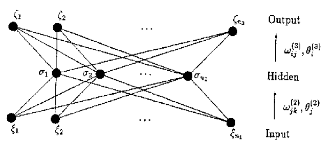
Figure 2: A three-layer feed-forward neural network consisting of input, hidden and output layers.

Multilayer feed-forward neural networks can be viewed as functions $F$ from $\mathbb{R}^{n_{1}}\rightarrow\mathbb{R}^{n_{L}}$, parametrized by weights, thresholds and activation function,

$$\boldsymbol{\xi}^{(L)}=F\left[\boldsymbol{\xi}^{(1)};\{w_{ij}^{(l)}\},\{\theta_{i}^{(l)}\};g\right].$$ (10)

For given activation function, the parameters can be tuned in such a way that the neural network reproduces any continuous function. The behaviour of a neural network is determined by the joint behaviour of all its connections and thresholds, and it can thus be built to be redundant, in the sense that modifying, adding or removing a neuron has little impact on the final output. Because of these reasons, neural networks can be considered to be robust, unbiased universal approximants.

3.2 Learning process for neural networks

The usefulness of neural networks is due to the availability of a training algorithm. This algorithm allows one to select the values of weights and thresholds such that the neural network reproduces a given set of input–output data (or patterns). This procedure is called ‘learning’ since, unlike a standard fitting procedure, there is no need to know in advance the underlying rule which describes the data. Rather, the neural network generalizes the examples used to train it.

The learning algorithm which we shall use is known as supervised training by back-propagation. Consider a set of input-output patterns $({\bf x},{\bf z})$ which we want the neural network to learn. The state of the neural network is generically given by

$$\xi_{i}^{(l)}=g(h_{i}^{(l)}),\quad\quad h_{i}^{(l)}=\sum_{j=1}^{n_{l-1}}\omega_{ij}^{(l-1)}\,\xi_{j}^{(l-1)}-\theta_{i}^{(l)};\qquad i=1,\dots,n_{l},\quad l=1,\dots,L.$$ (11)

Input–output patterns correspond to pairs of states of the first and last layers, which we shall denote as

$$\matrix{{\bf x}&=&\boldsymbol{\xi}^{(1)}\,,\cr{\bf o}({\bf x})&=&\boldsymbol{\xi}^{(L)}.}$$ (12)

The goal of the training is to learn from a given set of data patterns, which consist of associations of a given input with a desired output. For any given values of the weights and thresholds, define the error function

$$E[{\omega,\theta}]\equiv{{1}\over{2}}\sum_{A=1}^{n_{p}}\sum_{i=1}^{n_{L}}(o_{i}({\bf x}^{A})-z_{i}^{A})^{2}\,,$$ (13)

where $n_{p}$ is the number of data, i.e., the number of input–output patterns. The error Eq. (13) is the quadratic deviation between the actual and the desired output of the network, measured over the training set.

Given a fixed activation function $g$, Eq. (10), the error function is a function of the weights and thresholds. It can be minimized by looking for the direction of steepest descent in the space of weights and thresholds, and modifying the parameters in that direction:

$$\delta\omega_{ij}^{(l)} = -\eta{{\partial E}\over{\partial\omega_{ij}^{(l)}}}\,,$$

$$\delta\theta_{i}^{(l)} = -\eta{{\partial E}\over{\partial\theta_{i}^{(l)}}},$$

where $\eta$ fixes the rate of descent, i.e. the ‘learning rate’.

The nontrivial result on which training is based is that it can be shown that the steepest descent direction is given by the following recursive expression:

$${{\partial E}\over{\partial\omega_{ij}^{(l)}}} = \sum_{A=1}^{n_{p}}\Delta_{i}^{(l)A}\xi_{j}^{(l-1)A};\qquad i=1,\ldots,n_{l},\quad j=1,\ldots,n_{l-1}\,,$$

$${{\partial E}\over{\partial\theta_{i}^{(l)}}} = -\sum_{A=1}^{n_{p}}\Delta_{i}^{(l)A},\qquad i=1,\ldots,n_{l},$$ (15)

where the information on the goodness of fit is fed to the last layer through

$$\Delta_{i}^{(L)A}=g^{\prime}\left(h_{i}^{(L)A}\right)[o_{i}({\bf x}^{A})-z_{i}^{A}]\,$$ (16)

and then it is back-propagated to the rest of the network by

$$\Delta_{j}^{(l-1)A}=g^{\prime}\left(h_{j}^{(l-1)A}\right)\sum_{i=1}^{n_{l}}\Delta_{i}^{(l)A}\omega_{ij}^{(l)}\,.$$ (17)

The back-propagation algorithm then consists of the following steps:

1. initialize all the weights and thresholds randomly, and choose a small value for the learning rate $\eta$;

2. run a pattern ${\bf x}^{A}$ of the training set and store the activations of all the units;

3. calculate $\Delta_{i}^{(L)A}$ Eq. (16), and then back-propagate the error using Eq. (17);

4. compute the contributions to $\delta\omega_{ij}^{(l)}$ and $\delta\theta_{i}^{(l)}$ substituting Eq. (15) in Eq. (3.2);

5. update weights and thresholds.

The procedure is iterated until a suitable convergence criterion is fulfilled: for instance, if the value of the error function Eq. (13) stops decreasing. The back–propagation can be performed in “batched” or “on–line” modes. In the former case, weights and thresholds are only updated after all patterns have been presented to the network, as indicated in Eq. (15). In the latter case, the update is performed each time a new pattern is processed. Generally, on-line processing leads to faster learning, is less prone to getting trapped into local minima, and it is thus preferable if the number of data is reasonably small (i.e. $\mathrel{\mathchoice{\lower 0.86108pt\vbox{\halign{$\m@th\displaystyle\hfil#$\cr<\crcr\sim\crcr}}}{\lower 0.86108pt\vbox{\halign{$\m@th\textstyle\hfil#$\cr<\crcr\sim\crcr}}}{\lower 0.86108pt\vbox{\halign{$\m@th\scriptstyle\hfil#$\cr<\crcr\sim\crcr}}}{\lower 0.86108pt\vbox{\halign{$\m@th\scriptscriptstyle\hfil#$\cr<\crcr\sim\crcr}}}}10^{3}$).

It is clear that back-propagation seeks minima of the error function given in Eq. (13), but it cannot ensure that the global minimum is found. Several modifications have been proposed to improve the algorithm so that local minima are avoided. One of the most successful, simple and commonly used variants is the introduction of a ‘momentum’ term. This means that Eq. (3.2) is replaced by

$$\delta\omega_{ij}^{(l)} = -\eta{{\partial E}\over{\partial\omega_{ij}^{(l)}}}+\alpha\ \delta\omega_{ij}^{(l)}(\rm{last})$$

$$\delta\theta_{i}^{(l)} = -\eta{{\partial E}\over{\partial\theta_{i}^{(l)}}}+\alpha\ \delta\theta_{i}^{(l)}(\rm{last})$$ (18)

where “last” denotes the values of the $\delta\omega_{ij}^{(l)}$ and $\delta\theta_{i}^{(l)}$ used in the previous updating of the weights and thresholds. The parameter $\alpha$ (‘momentum’) must be a positive number smaller than 1.

Also, it may be convenient to choose a more general form of the error function, such as

$$E[{\omega,\theta}]\equiv\sum_{A,B=1}^{n_{p}}\sum_{i}^{n_{L}}(o_{i}({\bf x}^{A})-z_{i}^{A})V_{AB}(o_{i}({\bf x}^{B})-z_{i}^{B})\,,$$ (19)

where $V_{AB}$ is a $n_{p}\times n_{p}$ matrix which can accommodate weights and correlations between data, such as, typically, the inverse of the covariance matrix. If the matrix $V_{AB}$ is diagonal, the back–propagation algorithm is essentially unchanged, up to a rescaling of $\Delta_{i}^{(L)A}$ Eq. (16) by the corresponding matrix element $V_{AA}$. However, if the matrix $V_{AB}$ is not diagonal (i.e. the data are correlated), Eq. (16) must be substituted by a non–local expression which involves the sum over all correlated data. Clearly, in this case batched training is preferable, so that all correlated patterns are shown to the net before the weights and thresholds are updated.

4 Neural structure functions

4.1 General Strategy

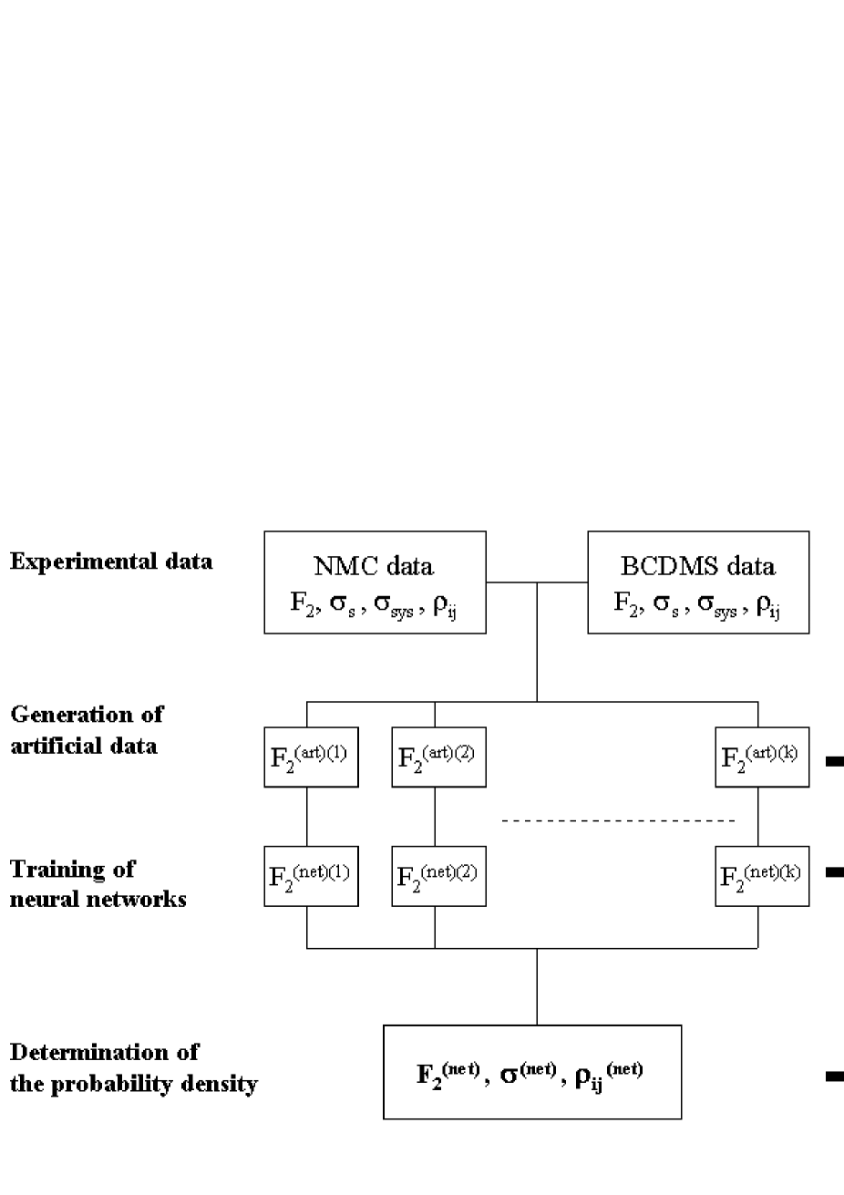
Figure 3: Flow chart for the construction of the parametrization of structure functions

We now describe in detail the strategy which we shall follow in order to construct a neural parametrization of structure functions (see Figure 3). As discussed in Sect. 2.2, the basic idea of our approach consists of constructing a representation of the probability measure in the space of structure functions. We do this in two steps: first, we generate a sampling of this measure based on the available data, and then we interpolate between these points using neural networks. The final set of neural networks is the sought–for representation of the probability measure.

The first step consists of generating a Monte Carlo set of ‘pseudo–data’, i.e.  $N_{rep}$ replicas of the original set of $N_{dat}$ data points:

$$F^{(art)(k)}_{i};\qquad k=1,\dots,N_{rep},\quad i=1,\dots,N_{dat},$$ (20)

where the subscript $i$ is a shorthand for $(x_{i},Q_{i}^{2})$. The $N_{rep}$ sets of $N_{dat}$ points are distributed according to an $N_{dat}$–dimensional multigaussian distribution about the original points, with expectation values equal to the central experimental values, and error and covariance equal to the corresponding experimental quantities. Because [17, 18] the distribution of the experimental data coincides (for a flat prior) with the probability distribution of the value of the structure function $F_{2}$ at the points where it has been measured, this Monte Carlo set gives a sampling of the probability measure at those points. We can then generate arbitrarily many sets of pseudo–data: the number of sets $N_{rep}$ can be chosen to be large enough that all relevant properties of the probability distribution of the data (such as errors and correlations) are correctly reproduced by the given sample. We will perform a number of tests in order to determine the optimal value of $N_{rep}$, which will be discussed in Sect. 4.2.

The second step consists of training $N_{rep}$ neural networks, one for each set of $N_{dat}$ pseudo–data. The key issue here is the choice of a suitable error function Eq. (19). A possibility would be to use the simplest unweighted form Eq. (13):

$$E^{(k)}[\omega,\theta]=\sum_{i=1}^{N_{dat}}{\left(F^{(art)(k)}_{i}-F^{(net)(k)}_{i}\right)^{2}},$$ (21)

where $F_{i}^{(net)(k)}$ is the output of the neural network for the input values of $(x,\,Q^{2})$ corresponding to the $i^{th}$ data point. Then, with suitable choices of architecture and training, we can achieve a value of the error such that $E/N_{dat}$ is much smaller than the typical experimental uncertainty on each point. In other words, the trained net will then go on top of each point, on the scale of experimental errors. Therefore, it will reproduce the sampling of the probability distribution at the measured points, and interpolate between them, thus achieving our goal. In fact, this happens even if $E/N_{dat}$ is not significantly smaller than the experimental uncertainty, provided only that for each point $i$ the shifts $\delta_{i}^{(k)}\equiv F^{(net)(k)}_{i}-F^{(art)(k)}_{i}$ are distributed as uncorrelated random variables with zero mean as $k$ runs over replicas. Then, it is easy to see that the distribution of $F^{(net)(k)}_{i}$ has the same average, variance, and point–to–point correlations as the distribution of $F^{(art)(k)}_{i}$.

This is however not an optimal solution in that it does not fully exploit the available physical information. To understand this, assume the value of the structure function at the same $(x,\,Q^{2})$ point is measured by two different experiments. If the measurements are independent, they are uncorrelated. However, since they determine the same physical observable, they cannot be treated as independent, and they must in fact be combined to give a single determination, with an error that it is smaller than either of the two measurements. Now, it is clear that if the structure function is measured at two points which are very close in $(x,\,Q^{2})$, then the value of the structure function at these points are likewise not independent: even though we do not know the functional form of the structure function, obvious QCD arguments imply that such a functional form exists, and it is continuous. Hence, by continuity, two neighbouring points cannot be treated as independent samplings of a probability distribution, and should be combined. This combined distribution has a variance which is in general smaller than its sampling at fixed points.

This reduction in variance is automatically achieved when fitting a given function to the data: if we fit a function to each set of pseudo–data, then as the pseudo–data span their multigaussian space, the best–fit values of the parameters which parametrize the function vary over their own space. As the number of data points is increased, the variance of these parameters decreases. For instance, assuming for the sake of argument a multilinear law with $k$ parameters, with $k$ data points all parameters can be determined with an error which can be found by error propagation, but with $N_{dat}>k$ points this error is reduced by a factor $1/\sqrt{N_{dat}-k}$. More in general, if the number of data exceeds the number of parameters, the error on the parameters will be reduced by a factor which is bounded by the so–called RCF inequality [18]; if there exists an estimate of the parameters which saturates this bound (as in the multilinear case), then it can be found by maximum–likelihood.

We are thus led to think that the optimal strategy consists of choosing as an error function the log-likelihood function for the given data. In this case, the matrix $V_{AB}$ in Eq. (19) is identified with the experimental covariance matrix, so the error function is

$$E^{(k)}[\omega,\theta]=\sum_{i,j=1}^{N_{dat}}{\left(F^{(art)(k)}_{i}-F^{(net)(k)}_{i}\right)\mathrm{cov}_{ij}^{-1}\left(F^{(art)(k)}_{j}-F^{(net)(k)}_{j}\right)},$$ (22)

where $\mathrm{cov}_{ij}$ is the covariance matrix defined in Eq. (3). In such case, if we assume that after training the neural network can capture — at least locally — the underlying functional form, then a maximum–likelihood determination of its parameters leads to a distribution of neural networks with a smaller uncertainty than that based on the minimization of the naive error function Eq. (21).

In practice, however, this choice turns out not to be viable. Indeed, as discussed in Sect. 3.2, the back–propagation algorithm with the error function Eq. (22) is non–local, and has poor convergence properties, especially when the number of data is large, as in our case. Note that this difficulty is related to the number of correlated data points, and thus it persists even if the number of correlated systematics is actually small, despite the fact that in such case the inversion of the correlation matrix is not a problem [5].

A strategy that is both physically effective and numerically viable consists instead of choosing as an error function the log–likelihood calculated from uncorrelated statistical errors, namely

$$E^{(k)}[\omega,\theta]=\sum_{i=1}^{N_{dat}}{{\left(F^{(art)(k)}_{i}-F^{(net)(k)}_{i}\right)^{2}}\over{{\sigma^{(exp)}_{i,s}}^{2}}}\,,$$ (23)

where $\sigma^{(exp)}_{i,s}$ is the statistical error on the $i^{th}$ data point. Because the error function is now diagonal, use of the back–propagation algorithm is no longer problematic. In order to understand the effect of minimizing the error function Eq. (23), write the probability distribution of the $i^{th}$ data point as $k$ runs over replicas as

$$F_{i}^{(art)(k)}=F_{i}^{(exp)}+\sum_{p=1}^{N_{sys}}r_{i,p}^{(k)}\sigma_{i,p}+r_{i,s}^{(k)}\sigma_{i,s},$$ (24)

where $F_{i}^{(exp)}$ is the experimental value, all $r^{(k)}$ are distributed in $k$ as univariate gaussian random numbers with zero mean, $\sigma_{s}$ is the statistical error, and $\sigma_{p}$ are the $N_{sys}$ systematics. Whereas there are $N_{dat}$ independent $r_{i,s}$, the number of independent variables $r_{i,p}$ for each $p$ is smaller, in that there is one single random variable $r_{i,p}$ for all correlated data points. The maximum–likelihood fit of the error function Eq. (23) to a set of data distributed according to Eq. (24) determines the values of $F^{(net)}_{i}$ which best fit the distribution of

$$F_{i}^{(sys)(k)}\equiv F_{i}^{(exp)}+\sum_{p=1}^{N_{sys}}r_{i,p}^{(k)}\sigma_{i,p}.$$ (25)

In this case, the distribution of best–fit functional neural networks as $k$ runs over replicas will have the smaller uncertainty which is obtained by maximum–likelihood combination of the statistical errors. However, it will still reproduce the (unimproved) systematic errors as $k$ runs over the Monte Carlo sample. The distribution of systematic errors will remain unbiased, provided only that for each point $i$ the distribution of best–fit values of $F^{(net)(k)}_{i}$ about $F^{(art)(k)}_{i}$ as $k$ runs over replicas is such that $F^{(net)(k)}_{i}$ is uncorrelated to $r_{i,p}^{(k)}$. In other words, the best–fit nets provides a probability distribution which optimally combines statistical errors, but reproduces the systematic errors of the Monte Carlo sample.

Just as in the first step, also in this second step of the procedure it will be necessary to verify whether the number of replicas is large enough that the statistical properties of the distributions are properly reproduced. Furthermore, it will be necessary to verify that the network fitting procedure did not introduce any bias, and specifically that if the statistical variance is reduced this is due to having combined data points, and not to a bias of the fitting procedure. To this purpose, we will develop a number of statistical tools which will be discussed in Sect. 5.1 when presenting our results.

At the end of our procedure, we obtain a set of $N_{rep}$ trained neural networks which provides us with a representation of the probability measure in the space of structure functions, and thus it allows us to determine any observable by averaging with this measure, Eq. (6). In particular, estimators for expectation values, errors and correlations are

$$\Big{\langle}F^{(net)}_{i}\Big{\rangle}_{rep}={{1}\over{N_{rep}}}\sum_{k=1}^{N_{rep}}F_{i}^{(net)(k)}$$ (26)

$$\sigma^{(net)}_{i}=\sqrt{\Big{\langle}\left(F^{(net)}_{i}\right)^{2}\Big{\rangle}_{rep}-\Big{\langle}F^{(net)}_{i}\Big{\rangle}_{rep}^{2}}$$ (27)

$$\rho^{(net)}_{ij}={{\Big{\langle}F^{(net)}_{i}\,F^{(net)}_{j}\Big{\rangle}_{rep}-\Big{\langle}F^{(net)}_{i}\Big{\rangle}_{rep}\Big{\langle}F^{(net)}_{j}\Big{\rangle}_{rep}}\over{\sigma^{(net)}_{i}\,\sigma^{(net)}_{j}}}\,,$$ (28)

where $i$, $j$ denote two pairs of values $(x_{i},Q^{2}_{i})$, $(x_{j},Q^{2}_{j})$ (not necessarily in the original data set). More in general, any functional average, defined by Eq. (6), can be estimated by

$$\Big{\langle}{\cal F}\left[F_{2}(x,Q^{2})\right]\Big{\rangle}={{1}\over{N_{rep}}}\sum_{k=1}^{N_{rep}}{\cal F}\left[{F_{2}}^{(net)(k)}(x,Q^{2})\right].$$ (29)

4.2 Generation of artificial data

The Monte Carlo set of pseudo–data can be generated by using equations of the form of (24). In particular, for the NMC experiment we have

$$F_{i}^{(art)\,(k)} = (1+r_{7}^{(k)}\,\sigma_{N})\Bigg{[}F_{i}^{(exp)}$$

$$+ {{r_{i,1}^{(k)}\,E_{i}+r_{i,2}^{(k)}\,E^{\prime}_{i}+r_{i,3}^{(k)}\,AC_{i}+r_{i,4}^{(k)}\,RC_{i}+r_{i,5}^{(k)}\,RE_{i}}\over{100}}F_{i}^{(exp)}+r_{i,s}^{(k)}\,\sigma_{i,s}\Bigg{]}\,,$$

where each $r_{i,p}^{(k)}$ is distributed as an univariate gaussian random number with zero mean over the replica sample (i.e., as $k$ varies), $F_{i}^{(exp)}$ is the central experimental value, and the various sources of systematics were discussed in Sect. 2.1.1. Since statistical errors are uncorrelated, there is an independent $r_{i,s}$ for each data point. Correlated systematics are correctly reproduced by taking the same $r_{3}$ and $r_{5}$ for all data corresponding to all energies and targets, the same $r_{4}$ for all targets, and the same $r_{1}$, $r_{2}$ and $r_{7}$ for all targets.

Likewise, for BCDMS we have

$$F_{i}^{(art)\,(k)} = (1+r_{5}^{(k)}\,\sigma_{N})\sqrt{1+r_{i,6}^{(k)}\,\sigma_{N_{t}}}\sqrt{1+r_{i,7}^{(k)}\,\sigma_{N_{b}}}\Bigg{[}F_{i}^{(exp)}$$

$$+ {{r_{i,1}^{(k)}\,f_{b}+r_{i,2}^{(k)}\,f_{i,s}+r_{i,3}^{(k)}\,f_{i,r}}\over{100}}F_{i}^{(exp)}+r_{i,s}^{(k)}\,\sigma_{s}^{i}\Bigg{]}\,,$$

where now $r_{1}$,$r_{2}$,$r_{3}$ and $r_{5}$ take the same value for all data (all energies and targets), $r_{6}$ is fixed for a given target, $r_{7}$ is fixed for given beam energy.

In order to determine a suitable value of $N_{rep}$, we now compare expectation values, variance and correlations of the pseudo–data set with the corresponding input experimental values, as a function of the number of replicas. A graphical comparison is shown in Figure. 4, where we display scatter plots of the central values, errors and correlation coefficients for samples of 10, 100 and 1000 replicas, for the proton, deuteron, and nonsinglet structure functions.

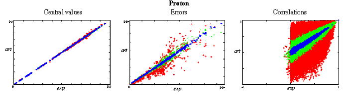
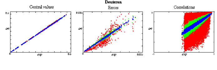
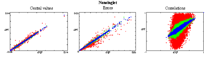
Figure 4: $\Big{\langle}F^{(art)}_{i}\Big{\rangle}_{rep}$ vs. $\bar{F}^{(exp)}_{i}$, $\Big{\langle}\sigma^{(art)}_{i}\Big{\rangle}_{rep}$ vs. $\bar{\sigma}^{(exp)}_{i}$ and $\Big{\langle}\rho_{ij}^{(art)}\Big{\rangle}_{rep}$ vs. $\rho_{ij}^{(exp)}$ with $N_{rep}=$ 10 (red), 100 (green) and 1000 (blue) replicas.

$F_{2}^{p}$
$N_{rep}$	10	100	1000
$\Big{\langle}V\left[\Big{\langle}F^{(art)}\Big{\rangle}_{rep}\right]\Big{\rangle}_{dat}$	$1.8\times 10^{-5}$	$1.7\times 10^{-6}$	$1.3\times 10^{-7}$
$\Big{\langle}PE\left[\Big{\langle}F^{(art)}\Big{\rangle}_{rep}\right]\Big{\rangle}_{dat}$	1.3%	0.4%	0.1%
$r[F^{(art)}]$	0.99949	0.99995	0.99999
$\Big{\langle}V[\sigma^{(art)}]\Big{\rangle}_{dat}$	$8.0\times 10^{-5}$	$2.4\times 10^{-5}$	$7.0\times 10^{-6}$
$\Big{\langle}PE[\sigma^{(art)}]\Big{\rangle}_{dat}$	40%	11%	4%
$\Big{\langle}\sigma^{(art)}\Big{\rangle}_{dat}$	0.0102	0.0114	0.0114
$r[\sigma^{(art)}]$	0.900	0.987	0.999
$\Big{\langle}V[\rho^{(art)}]\Big{\rangle}_{dat}$	0.0868	0.0056	0.0006
$\Big{\langle}\rho^{(art)}\Big{\rangle}_{dat}$	0.348	0.384	0.378
$r[\rho^{(art)}]$	0.623	0.960	0.996
$\Big{\langle}V[\mathrm{cov}^{(art)}]\Big{\rangle}_{dat}$	$5.5\times 10^{-9}$	$4.6\times 10^{-10}$	$4.7\times 10^{-11}$
$\Big{\langle}\mathrm{cov}^{(art)}\Big{\rangle}_{dat}$	$3.4\times 10^{-5}$	$3.8\times 10^{-5}$	$3.8\times 10^{-5}$
$r[\mathrm{cov}^{(art)}]$	0.519	0.906	0.987

Table 1: Comparison between experimental and generated artificial data for the proton structure function. The experimental data have $\Big{\langle}\sigma^{(exp)}\Big{\rangle}_{dat}=0.0116$, $\Big{\langle}\rho^{(exp)}\Big{\rangle}_{dat}=0.382$ and $\Big{\langle}\mathrm{cov}^{(exp)}\Big{\rangle}_{dat}=3.8\times 10^{-5}$.

$F_{2}^{d}$
$N_{rep}$	10	100	1000
$\Big{\langle}V\left[\Big{\langle}F^{(art)}\Big{\rangle}_{rep}\right]\Big{\rangle}_{dat}$	$9.2\times 10^{-6}$	$9.1\times 10^{-7}$	$9.7\times 10^{-8}$
$\Big{\langle}PE\left[\Big{\langle}F^{(art)}\Big{\rangle}_{rep}\right]\Big{\rangle}_{dat}$	1.1%	0.3%	0.1%
$r[F^{(art)}]$	0.99976	0.99998	0.99999
$\Big{\langle}V[\sigma^{(art)}]\Big{\rangle}_{dat}$	$5.3\times 10^{-5}$	$1.5\times 10^{-5}$	$4.0\times 10^{-6}$
$\Big{\langle}PE[\sigma^{(art)}]\Big{\rangle}_{dat}$	39%	11%	3%
$\Big{\langle}\sigma^{(art)}\Big{\rangle}_{dat}$	0.0095	0.0102	0.0102
$r[\sigma^{(art)}]$	0.857	0.990	0.999
$\Big{\langle}V[\rho^{(art)}]\Big{\rangle}_{dat}$	0.0923	0.0075	0.0007
$\Big{\langle}\rho^{(art)}\Big{\rangle}_{dat}$	0.374	0.310	0.310
$r[\rho^{(art)}]$	0.641	0.934	0.993
$\Big{\langle}V[\mathrm{cov}^{(art)}]\Big{\rangle}_{dat}$	$2.6\times 10^{-9}$	$2.5\times 10^{-10}$	$2.3\times 10^{-11}$
$\Big{\langle}\mathrm{cov}^{(art)}\Big{\rangle}_{dat}$	$3.3\times 10^{-5}$	$3.3\times 10^{-5}$	$3.2\times 10^{-5}$
$r[\mathrm{cov}^{(art)}]$	0.568	0.932	0.992

Table 2: Comparison between experimental and generated artificial data for the deuteron structure function. The experimental data have $\Big{\langle}\sigma^{(exp)}\Big{\rangle}_{dat}=0.0102$, $\Big{\langle}\rho^{(exp)}\Big{\rangle}_{dat}=0.313$ and $\Big{\langle}\mathrm{cov}^{(exp)}\Big{\rangle}_{dat}=3.3\times 10^{-5}$.

$F_{2}^{p}-F_{2}^{d}$
$N_{rep}$	10	100	1000
$\Big{\langle}V\left[\Big{\langle}F^{(art)}\Big{\rangle}_{rep}\right]\Big{\rangle}_{dat}$	$1.4\times 10^{-5}$	$1.8\times 10^{-6}$	$2.7\times 10^{-7}$
$\Big{\langle}PE\left[\Big{\langle}F^{(art)}\Big{\rangle}_{rep}\right]\Big{\rangle}_{dat}$	35%	11%	4%
$r[F^{(art)}]$	0.980	0.998	0.999
$\Big{\langle}V[\sigma^{(art)}]\Big{\rangle}_{dat}$	$6.6\times 10^{-5}$	$2.19\times 10^{-5}$	$7.8\times 10^{-6}$
$\Big{\langle}PE[\sigma^{(art)}]\Big{\rangle}_{dat}$	35%	12%	4%
$\Big{\langle}\sigma^{(art)}\Big{\rangle}_{dat}$	0.0101	0.0114	0.0114
$r[\sigma^{(art)}]$	0.927	0.991	0.999
$\Big{\langle}V[\rho^{(art)}]\Big{\rangle}_{dat}$	0.1133	0.0094	0.0010
$\Big{\langle}\rho^{(art)}\Big{\rangle}_{dat}$	0.1112	0.0990	0.0946
$r[\rho^{(art)}]$	0.405	0.816	0.971
$\Big{\langle}V[\mathrm{cov}^{(art)}]\Big{\rangle}_{dat}$	$5.1\times 10^{-9}$	$5.8\times 10^{-10}$	$6.0\times 10^{-11}$
$\Big{\langle}\mathrm{cov}^{(art)}\Big{\rangle}_{dat}$	$7.3\times 10^{-6}$	$9.0\times 10^{-6}$	$8.7\times 10^{-6}$
$r[\mathrm{cov}^{(art)}]$	0.346	0.791	0.972

Table 3: Comparison between experimental and generated artificial data for the nonsinglet structure function. The experimental data have $\Big{\langle}\sigma^{(exp)}\Big{\rangle}_{dat}=0.0114$, $\Big{\langle}\rho^{(exp)}\Big{\rangle}_{dat}=0.090$ and $\Big{\langle}\mathrm{cov}^{(exp)}\Big{\rangle}_{dat}=8.4\times 10^{-6}$.

A more quantitative comparison can be performed defining the following quantities

• Average over the number of replicas for each experimental point $i$ (i.e. a pair of values of $x$ and $Q^{2}$)

  $$\Big{\langle}F^{(art)}_{i}\Big{\rangle}_{rep}={{1}\over{N_{rep}}}\sum_{k=1}^{N_{rep}}F_{i}^{(art)(k)}\,.$$ (32)

  Variance of $\langle F^{(art)}_{i}\rangle_{rep}$

  $$\sigma^{(art)}_{i}=\sqrt{\Big{\langle}\left(F^{(art)}_{i}\right)^{2}\Big{\rangle}_{rep}-\Big{\langle}F_{i}^{(art)}\Big{\rangle}_{rep}^{2}}\,.$$ (33)

  Correlation and covariance of two points

  $$\rho^{(art)}_{ij} = {{\Big{\langle}F^{(art)}_{i}\,F^{(art)}_{j}\Big{\rangle}_{rep}-\Big{\langle}F^{(art)}_{i}\Big{\rangle}_{rep}\Big{\langle}F^{(art)}_{j}\Big{\rangle}_{rep}}\over{\sigma^{(art)}_{i}\,\sigma^{(art)}_{j}}},$$ (34)

  $$\mathrm{cov}^{(art)}_{ij} = \rho^{(art)}_{ij}\sigma^{(art)}_{i}\sigma^{(art)}_{j}.$$ (35)

  These quantities provide the estimators of the experimental values, errors, and correlation which one extracts from the sample of artificial data.

• Mean variance and mean percentage error on central values over the number of points $N_{dat}$

  $$\Big{\langle}V\left[\Big{\langle}F^{(art)}\Big{\rangle}_{rep}\right]\Big{\rangle}_{dat} = {{1}\over{N_{dat}}}\sum_{i=1}^{N_{dat}}\left(\Big{\langle}F^{(art)}_{i}\Big{\rangle}_{rep}-F^{(exp)}_{i}\right)^{2}$$ (36)

  $$\Big{\langle}PE\left[\Big{\langle}F^{(art)}\Big{\rangle}_{rep}\right]\Big{\rangle}_{dat} = {{1}\over{N_{dat}}}\sum_{i=1}^{N_{dat}}\left|{{\Big{\langle}F^{(art)}_{i}\Big{\rangle}_{rep}-F^{(exp)}_{i}}\over{F^{(exp)}_{i}}}\right|\,.$$ (37)

  We can similarly define $\Big{\langle}V[\sigma^{(art)}]\Big{\rangle}_{dat}$, $\Big{\langle}PE[\sigma^{(art)}]\Big{\rangle}_{dat}$, $\Big{\langle}V[\rho^{(art)}]\Big{\rangle}_{dat}$ and $\Big{\langle}V[\mathrm{cov}^{(art)}]\Big{\rangle}_{dat}$. These estimators indicate how close the averages over generated data are to the experimental values.

• Scatter correlation:

  $$r[F^{(art)}]={{\Big{\langle}F^{(exp)}\,\Big{\langle}F^{(art)}\Big{\rangle}_{rep}\Big{\rangle}_{dat}-\Big{\langle}F^{(exp)}\Big{\rangle}_{dat}\Big{\langle}\Big{\langle}F^{(art)}\Big{\rangle}_{rep}\Big{\rangle}_{dat}}\over{\sigma_{s}^{(exp)}\,\sigma_{s}^{(art)}}}\,.$$ (38)

  where the scatter variances are defined as

  $$\sigma_{s}^{(exp)} = \Big{\langle}(F^{(exp)})^{2}\Big{\rangle}_{dat}-\left(\Big{\langle}F^{(exp)}\Big{\rangle}_{dat}\right)^{2}$$

  $$\sigma_{s}^{(art)} = \Big{\langle}\left(\Big{\langle}F^{(art)}\Big{\rangle}_{rep}\right)^{2}\Big{\rangle}_{dat}-\left(\Big{\langle}\Big{\langle}F^{(art)}\Big{\rangle}_{rep}\Big{\rangle}_{dat}\right)^{2}.$$ (39)

  Similarly we define $r[\sigma^{(art)}]$, $r[\rho^{(art)}]$ and $r[\mathrm{cov}^{(art)}]$. The scatter correlation indicates the size of the spread of data around a straight line in the scatter plots of Figure 4. Specifically, $r[\sigma^{(net)}]=1$ implies that $\langle\sigma^{(net)}_{i}\rangle$ is proportional to $\sigma^{(exp)}_{i}$ (and similarly for $r[F^{(net)}]$ etc.). Note that the scatter correlation and scatter variance are not related to the variance and correlation Eqs. (33-35) or averages thereof.

• Average variance:

  $$\Big{\langle}\sigma^{(art)}\Big{\rangle}_{dat}={{1}\over{N_{dat}}}\sum_{i=1}^{N_{dat}}\sigma^{(art)}_{i}.$$ (40)

  Similarly we can define $\Big{\langle}\rho^{(art)}\Big{\rangle}_{dat}$ and $\Big{\langle}\mathrm{cov}^{(art)}\Big{\rangle}_{dat}$. Analogously, we can define the corresponding experimental quantities

  $$\Big{\langle}\sigma^{(exp)}\Big{\rangle}_{dat}={{1}\over{N_{dat}}}\sum_{i=1}^{N_{dat}}\sigma^{(exp)}_{i}$$ (41)

  where $\sigma^{(exp)}_{i}$ is the experimental error on the $i^{th}$ data point, an so forth. These quantities are interesting because even if the scatter correlation $r$ Eq. (38) is very close to one (so all points in the scatter plots Figure 4 lie on a straight line), there could still be a systematic bias in the estimators Eqs. (32-35). For example, if for all points $i$ the variance $\sigma_{i}^{(art)}=\lambda\sigma_{i}^{(exp)}$, then $r[\sigma^{(art)}]=1$, but $\Big{\langle}\sigma^{(art)}\Big{\rangle}_{dat}=\lambda\Big{\langle}\sigma^{(exp)}\Big{\rangle}_{dat}$.

The values of these quantities for samples of 10, 100 and 1000 replicas and for the three structure functions under consideration are shown in Tables 1–3. From these tables, it can be seen that the scaling of the various quantities with $N_{rep}$ follows the standard behaviour of Gaussian Monte Carlo samples [18]. For instance, the variance on central values should scale as $1/N_{rep}$, while the variance on the errors should scale as $1/\sqrt{N_{rep}}$. This implies that a smaller sample is sufficient in order to achieve a given accuracy on means than it is required to reach the same accuracy on errors. Also, because $V[\rho^{(art)}]=[1-(\rho^{(exp)})^{2}]^{2}/N_{rep}$, the estimated correlation fluctuates more for small values of $\rho^{(exp)}$, and thus the average correlation $\langle\rho^{(art)}\rangle_{dat}$ tends to be larger than the corresponding experimental value $\langle\rho^{(exp)}\rangle_{dat}$. Notice finally that a larger sample is necessary in order to achieve a given percentage error on the nonsinglet than on the proton and deuteron. This is a consequence of the fact that the signal–to–noise ratio is smaller for the nonsinglet: the proton and deuteron structure functions are roughly of the same size, so the absolute value of the nonsinglet structure function is typically by about a factor 10 smaller.

Inspection of the tables shows that in order to reach average scatter correlations of 99% and percentage accuracies of a few percent on structure functions, errors and correlations a sample of about 1000 replicas is necessary. Notice in particular that with 1000 replicas the estimated correlation fluctuates about the true value, rather than systematically overshooting it.

4.3 Building and training Neural Networks

The choice of an optimal structure of the neural nets and of an optimal learning strategy cannot follow fixed rules and must be tailored to the specific problem. Here we summarize and motivate the specific choices which we made for our fits.

Number of layers

The optimal number of layers in a neural network depends on the complexity of the specific task it should perform. It can be proved [15] that any continuous function, no matter how complex, can be represented by a multilayer neural network with no more than three layers (input layer, a middle hidden layer, and output layer). However, in practice, using a single hidden layer may require a very large number of units in it. Thus, it can be more useful to have two hidden layers and a smaller number of neurons on each. We will only consider networks with two hidden layers.

Number of hidden units

The number of hidden units needed to approximate a given function ${\cal F}$ is related to the number of terms which are needed in an expansion of ${\cal F}$ over the basis of functions $g(x),\>g(g(x)),\>\dots$. There exist several techniques to determine the optimal number of units. Here we have taken a pragmatic approach. First, we carry out all the learning with a small number of units. Then, we restart the whole learning adding new units one by one, until stability of the error function is reached. In this way, an optimal architecture is found, which is large enough to reproduce faithfully the training patterns, but small enough that training is fast. The final results which we will present are obtained with the architecture (4–5–3–1). The reason why there are four input nodes will be discussed below.

Activation function

We have taken a sigmoid activation function Eq. (8). The sensitivity of the neural network can be enhanced by substituting the sigmoid activation function in the last layer with the identity (linear response). This avoids saturation of the last layer neurons and leaves space for more sensitive responses. For this reason, we have adopted linear response in the last layer. With these choices, and the architecture discussed above, the behaviour of the network is determined by the values of 47 free parameters (38 weights and 9 thresholds).

Rescaling

If the activation $\xi_{i}$ of input (output) node $i$ is numerically large, in order for the activation function to be in the nonlinear response regime, the weights $\omega_{ij}$ must be very small. However, if the activation is very large, the shifts Eq. (16) in the first stages of the learning process are also very large, thus leading to an erratic behaviour of the training process, unless the learning rate $\eta$ Eq. (15) is initially taken to be very small and then changed along the training. In order to avoid this, it is convenient to rescale both the input and the output data in such a way that that typical activations are $\xi_{i}\sim{\cal O}(1)$ for all $i$. In practice, we have rescaled all values of $(x,Q^{2})$ and the structure function $F_{2}$ in such a way that they span the range $0.1-0.9$. This ensures that activation functions are in the nonlinear regime when the absolute values of all the weights settle to values close to one.

Input

We have used as input variables $x$, $Q^{2}$, $\log x$ and $\log Q^{2}$. The choice of taking $\log x$ and $\log Q^{2}$ along with $x$ and $Q^{2}$ is motivated by the expectation that these are the variables upon which $F_{2}$ naturally depends. Note that this is not a source of theoretical bias: if this expectation turns out to be incorrect and these variables are useless, after training the neural network will simply disregard them. If, however, the expectation is correct this choice will speed up the training. We have checked that neural networks trained just with $x$ and $Q^{2}$ perform as well as the ones we use but need longer training times.

Theoretical assumptions

The only theoretical assumption on the shape of $F_{2}(x,Q^{2})$ produced by the neural nets is that it satisfies the kinematic bound $F_{2}(1,Q^{2})=0$ for all $Q^{2}$. In general, a constraint can be enforced by adding it to the error function Eq. (13), so that configurations that violate the constraint are unfavourably weighted. In our case, the constraint is local in $x$ and $Q^{2}$ so its implementation is straightfoward: it can be enforced by including in the data set a number of artificial data points which satisfy the constraint, with suitably tuned error. More general cosntraints, such as the momentum sum rule in a parton fit, would require a term which makes the error function nonlocal in $x$ and $Q^{2}$, and would thus make the training computationally more intensive.

We have thus added to the data set 10 artificial points at $x=1$ with equally spaced values of $Q^{2}$ on a linear scale between $20$ and $200$ GeV² (which ensures that the bound is respected even when extrapolating beyond the data region). The choice of the error on these points is very delicate: if it is too small, the neural networks will spend a significant fraction of their training time in learning these points. In such case, the kinematic constraint $F_{2}(x=1,Q^{2})=0$ is enforced with great accuracy, but at the expense of the fit to experimental data. We have thus taken the error on these points at $x=1$ to be of the same order of the smallest experimental error, namely, $10^{-3}$ for $F_{2}^{p}$ and $F_{2}^{d}$, and $\sqrt{2}\times 10^{-4}$ for $F_{2}^{p}-F_{2}^{d}$.

Training patterns

Since the number of data is reasonably small, we have adopted on–line training (see Sect. 3.2): weights are updated after each pattern is shown to the net. If the experimental data were shown to the net in a fixed order, a bias could arise, e.g. because of the regularity of some input patterns. Therefore, we have shown the data to the network using each time a random permutation of their order. Furthermore, the data are always shown at least $10^{4}$ times, in order to allow compensations of different variations. Because we use a pseudo–random number generator to compute permutations with periodicity $6\times 10^{6}$ which is smaller than a typical number of training cycles (see Sect. 5), there might still be periodic oscillations in behaviour of the best–fit network. However, we have checked that these oscillations do not significantly affect the fit.

Learning parameters

The choice of the learning rate $\eta$ Eq. (3.2) is particularly important: large values of $\eta$ lead to an unstable training process, while small values lead to slow training which may get trapped in local minima. In practice, it is convenient to vary the value of $\eta$ during the training: first, one looks for the region of the global minimum with a larger value of $\eta$. Once this region is located, the learning rate is reduced so that the probability of jumping away is small and it is then easier to deepen into the minimum. The momentum term $\alpha$ Eq. (3.2) is closely connected to the learning rate: an increase of $\alpha$ implies an increase of the effective learning rate. The optimum value of $\alpha$ depends on the updating procedure used.

For our training, we have chosen to first minimize the error function Eq. (21), and then switch to the minimization of Eq. (23): first we look for the rough location of the minimum, and then we refine its search. The first set of training (of the order of $10^{6}$ cycles) is performed with $\eta\sim 10^{-3}$, and the second (of the order of $10^{8}$ cycles) with $\eta\sim 10^{-8}$ (see Sect. 5). We will always take $\alpha=0.9$.

Convergence of the training procedure and parametrization bias

Figure 5: Fit of the nonsinglet structure function $F_{2}^{p}-F_{2}^{d}$ to a subset of BCDMS data points for increasing training lengths: insufficient training (left); ¡ normal training (middle); overlearning (right). The variable in abscissa is an arbitrary point number.

As the training of the neural network progresses, the neural net reproduces in a more and more detailed way the features of the given data set. It follows that the problem of determining convergence of the training procedure is tangled with the problem of avoiding a possible fitting bias. Indeed, if the net is too small or the training is too short, it will artificially smooth out physical fluctuations in the data, whereas if the training is too long, the net will also fit statistical noise (‘overlearning’). Convergence must be therefore assessed on the basis of a criterion which guarantees that the trained nets faithfully reproduce the local functional form of the data, without fitting statistical fluctuations, but also without imposing a smoothing bias. This issue is illustrated in Figure 5, where we show the form of a neural network with the architecture and features discussed above, trained to a small, arbitrarily chosen subset of 30 BCDMS data points for the structure function $F_{2}^{p}-F_{2}^{d}$, with increasingly long training cycles. With this small data set, chosen for the sake of illustration, the architecture of the nets is very redundant, and overlearning is easily achieved. The first plot (very short training) shows that the neural network strongly correlates data points, but it does not quite reproduce the behavior of data. The second plot corresponds to a longer training, which leads to a more or less ideal fit. In the last plot (very long training) the neural network follows the statistical fluctuations of individual data points (overlearning). Note that the abscissa in this plot is an arbitrary point number; jumps in the best–fit function are not significant and simply reflect the fact that points of neighbouring number might correspond to rather different values of $(x,Q^{2})$.

Extreme overlearning as displayed in Figure 5 can be avoided by using a number of parameters in the neural network which, while still being largely redundant so as to avoid parametrization bias, is significantly smaller than the number of points to be fitted. However, an accurate assessment of whether convergence has been reached can only be obtained by means of statistical indicators of the goodness of fit, tailored to the particular problem. These will be discussed in the next section. By means of such indicators, one may determine an optimal training length, and then subject all networks to training of this fixed length. This is more convenient than stopping the training on the basis of a convergence criterion, e.g. on the value of the error function, because this latter choice would tend to artificially damp statistical fluctuations of the pseudo–data sample, and it could thus lead to biased results.

5 Results

We will present results for the proton, deuteron and nonsinglet structure function $F_{2}$. We have decided to train a separate neural network for the nonsinglet in view of precision applications. This is because the proton and deuteron structure functions are roughly of the same size, while their difference is typically smaller by a factor 10. Hence, in order to achieve a 1% accuracy on $F_{2}^{p}-F_{2}^{d}$ we would need approximately a 0.1% accuracy on $F_{2}^{p}$ and $F_{2}^{d}$. An individual fit of the proton, deuteron, and nonsinglet allows us to achieve a comparable accuracy on all structure functions. After discussing the general aspects of the assessment of the quality of the fits, we will discuss separately the nonsinglet, proton and deuteron fits.

5.1 Fit assessment

As discussed in Sect. 4.1, the determination of the probability density in the space of structure function is based on the training of a neural network on each of the replicas of the original data set. We must therefore first, assess whether the training of each network is sufficient, and then verify that the set of networks represents the probability density of the data in a faithful and unbiased way.

The goodness of fit provided by each net is measured by the error function $E^{(k)}$ Eq. (23) which is minimized by the training process; the average goodness of fit is thus

$$\langle E\rangle_{rep}={{1}\over{N_{rep}}}\sum_{k=1}^{N_{rep}}{{1}\over{N_{dat}}}E^{(k)}$$ (42)

where we have further normalized to the number of data so that Eq. (42) coincides with the mean square error per data point per replica. We also define the normalized error function computed for the original set of data (rather than one of the replicas)

$$E^{(0)}={{1}\over{N_{dat}}}\sum_{i=1}^{N_{dat}}{{\left(F^{(exp)}_{i}-F^{(net)(0)}_{i}\right)^{2}}\over{{\sigma^{(exp)}_{i,s}}^{2}}},$$ (43)

where $F^{(net)(0)}_{i}$ is the prediction from a neural net trained on the set of central experimental values $F^{(exp)}_{i}$.

The estimator for the central value of each data point is given by the expectation value $\Big{\langle}F_{i}^{(net)}\Big{\rangle}_{rep}$ Eq. (26). The goodness of the fit to the original data provided by this estimator is

$$\chi^{2}={{1}\over{N_{dat}}}\sum_{i,\,j=1}^{N_{dat}}\left(\Big{\langle}F_{i}^{(net)}\Big{\rangle}_{rep}-F_{i}^{(exp)}\right)\mathrm{cov}^{-1}_{ij}\left(\Big{\langle}F_{j}^{(net)}\Big{\rangle}_{rep}-F_{j}^{(exp)}\right),$$ (44)

where $\mathrm{cov}_{ij}$ is the covariance matrix Eq. (3), and we have again normalized to the number of data points. Note that the number of degrees of freedom is not just the difference of $N_{dat}$ and the number of parameters of the neural network, because the neural network is by construction redundant (see Sect. 4.3): a network with a smaller number of parameters could lead to fits of the same quality, though with a longer training. However, the data points are about 500 (see Sect. 2) while the parameters of the net are about 50 (see Sect. 4.3), corresponding to some 10 or 20 truly independent degrees of freedom: hence, the expression Eq. (44) differs only by a few percent from the $\chi^{2}$ per degree of freedom.

In order to assess how well experimental errors are reproduced by their neural estimator Eq. (27) we define the corresponding average variance and percentage errors

$$\Big{\langle}V\left[\Big{\langle}F^{(net)}\Big{\rangle}_{rep}\right]\Big{\rangle}_{dat} = {{1}\over{N_{dat}}}\sum_{i=1}^{N_{dat}}\left(\Big{\langle}F^{(net)}_{i}\Big{\rangle}_{rep}-F^{(exp)}_{i}\right)^{2}$$ (45)

$$\Big{\langle}PE\left[\Big{\langle}F^{(net)}\Big{\rangle}_{rep}\right]\Big{\rangle}_{dat} = {{1}\over{N_{dat}}}\sum_{i=1}^{N_{dat}}\left|{{\Big{\langle}F^{(net)}_{i}\Big{\rangle}_{rep}-F^{(exp)}_{i}}\over{F^{(exp)}_{i}}}\right|\,.$$ (46)

We can similarly define percentage errors on the correlation and covariance $\Big{\langle}V[\rho^{(net)}]\Big{\rangle}_{dat}$ and $\Big{\langle}V[\mathrm{cov}^{(net)}]\Big{\rangle}_{dat}$.

A point–by–point measure of the agreement between network estimators and their experimental counterparts is provided by defining the scatter correlation of central values, in analogy to Eq. (38)

$$r[F^{(net)}]={{\Big{\langle}F^{(exp)}\Big{\langle}F^{(net)}\Big{\rangle}_{rep}\Big{\rangle}_{dat}-\Big{\langle}F^{(exp)}\Big{\rangle}_{dat}\Big{\langle}\Big{\langle}F^{(net)}\Big{\rangle}_{rep}\Big{\rangle}_{dat}}\over{\sigma_{s}^{(exp)}\,\sigma_{s}^{(net)}}}\,.$$ (47)

where the scatter variance of the network is

$$\sigma_{s}^{(net)}=\Big{\langle}\left(\Big{\langle}F^{(net)}\Big{\rangle}_{rep}\right)^{2}\Big{\rangle}_{dat}-\left(\Big{\langle}\Big{\langle}F^{(net)}\Big{\rangle}_{rep}\Big{\rangle}_{dat}\right)^{2}.$$ (48)

Similarly we define $r[\sigma^{(net)}]$, $r[\rho^{(net)}]$ and $r[\mathrm{cov}^{(net)}]$. As discussed in Sect. 4.2, the scatter correlation $-1\leq r\leq 1$ indicates how closely the network estimator follows its experimental counterpart as the index $i$ runs over experimental points. Specifically, $r[\sigma^{(net)}]\approx 1$ implies that $\langle\sigma^{(net)}_{i}\rangle$ is approximately proportional to $\sigma^{(exp)}_{i}$ (and similarly for $r[F^{(net)}]$ etc.). The coefficient of proportionality can then be found by comparing the average experimental variance Eq. (41) with the average network variance

$$\Big{\langle}\sigma^{(net)}\Big{\rangle}_{dat}={{1}\over{N_{dat}}}\sum_{i=1}^{N_{dat}}\sigma^{(net)}_{i}.$$ (49)

A substantial deviation of the scatter correlation from one indicates that the neural estimator is not following the pattern of experimental variations. This might indicate that the neural network is incapable of reproducing the shape of the data, or else that it is successfully reducing fluctuations in the data.

In practice, we are interested in the case in which the neural networks lead to a successful fit (i.e. with a good value of the $\chi^{2}$ (44)), while leading to a reduction of the variance, as discussed in Sect. 4.1, so that $\langle\sigma^{(net)}\rangle_{dat}<\langle\sigma^{(exp)}\rangle_{dat}$. Because we are minimizing the diagonal error function Eq. (23) and not the full likelihood, we cannot simply rely on the value of the average error $\langle E\rangle$ and the $\chi^{2}$ to assess the quality of the fit. Rather, we must verify that the distribution of systematic errors remains unbiased, and that if a reduction of the variance is observed it is not due to lack of flexibility of the neural network.

In order to test whether systematics are reproduced in an unbiased way, we notice that experimental correlations are entirely due to systematic errors, according to Eqs. (1-2). It follows from these equations and from the definition of covariance matrix (3) that if the networks reduce the statistical variance but reproduce the experimental systematics (as they ought to), then $\sigma_{i}^{(net)}<\sigma_{i}^{(exp)}$ and $\rho_{ij}^{(net)}>\rho_{ij}^{(exp)}$ but $\mathrm{cov}_{ij}^{(net)}\approx\mathrm{cov}_{ij}^{(exp)}$. So if $\mathrm{cov}^{(net)}$ and $\mathrm{cov}^{(exp)}$ are strongly correlated and have approximately the same mean, the systematics are reproduced in an unbiased way. Notice however that this condition is in general sufficient, but not necessary: for instance, more measurements at the same point from independent experiments have $\rho^{(exp)}=0$ identically, while $\rho^{(net)}=1$, so in this case $\mathrm{cov}^{(exp)}$ and $\mathrm{cov}^{(net)}$ cannot possibly be equal.

In order to test whether the variance reduction is due to the fact that the networks are distributed with smaller variance around the true experimental values, we construct a suitable estimator, assuming for simplicity all errors to be Gaussian. Consider a measurement value $m_{i}$ of $F_{2}$, where $i$ represents a pair of values $(x,Q^{2})$. For each measurement

$$m_{i}=t_{i}+\sigma_{i}\,s_{i}\,$$ (50)

where $s_{i}$ is a univariate Gaussian number with zero mean, $t_{i}$ is the true value of $F_{2}$, and $\sigma_{i}$ its error. The $k^{th}$ replica of generated data is then

$$g_{i}^{(k)}=m_{i}+r^{(k)}_{i}\,\sigma_{i}=t_{i}+(s_{i}+r^{(k)}_{i})\sigma_{i}\,,$$ (51)

where $r^{k}_{i}$ is also a univariate zero mean Gaussian random number. Assume now that the best–fit neural networks are distributed about the true values $t_{i}$ with an error $\hat{\sigma}_{i}$. For the $k^{th}$ neural network we have

$$n_{i}^{(k)}=t_{i}+{r^{\prime}}^{(k)}_{i}\,\hat{\sigma}_{i}\,,$$ (52)

where, assuming that the network is an unbiased estimator, ${r^{\prime}}^{(k)}_{i}$ have zero mean, and can be normalized to be univariate. Because the networks are determined by fitting to $g_{i}^{(k)}$, in general, ${r^{\prime}}^{(k)}_{i}$ will be correlated to $r^{(k)}_{i}$ and $t_{i}$.

If we assume that the number of replicas is large enough that $\Big{\langle}r^{(k)}_{i}\Big{\rangle}_{rep}=\Big{\langle}{r^{\prime}}^{(k)}_{i}\Big{\rangle}_{rep}=0$ and $\Big{\langle}(r^{(k)}_{i})^{2}\Big{\rangle}_{rep}=\Big{\langle}({r^{\prime}}^{(k)}_{i})^{2}\Big{\rangle}_{rep}=1$, while the number of data points is large enough that $\langle s_{i}\rangle_{dat}=0$ and $\langle s_{i}^{2}\rangle_{dat}=1$ we get the average error Eq. (42)

$$\langle E\rangle_{rep}=2+\langle(\hat{\sigma}/\sigma)^{2}\rangle_{dat}-2\langle\langle rr^{\prime}\rangle_{rep}(\hat{\sigma}/\sigma)\rangle_{dat},$$ (53)

where $\langle\rangle_{dat}$ denotes averaging with respect to data in one replica (index $i$) and $\langle\rangle_{rep}$ denotes averaging with respect to replicas (index $k$). Now, define a modified average error, where the prediction of the $k$–th network instead of being compared to the $k$–th replica (as in the average error proper Eq. (42)) are compared to the experimental data:

$$\widetilde{E}^{(k)} = \sum_{i=1}^{N_{dat}}{{\left(F^{(exp)}_{i}-F^{(net)(k)}_{i}\right)^{2}}\over{{\sigma^{(exp)}_{i,s}}^{2}}};$$ (54)

$$\langle\widetilde{E}\rangle_{rep} = {{1}\over{N_{rep}}}\sum_{k=1}^{N_{rep}}{{1}\over{N_{dat}}}\widetilde{E}^{(k)}$$ (55)

We get immediately

$$\langle\widetilde{E}\rangle_{rep}=1+\langle(\hat{\sigma}/\sigma)^{2}\rangle_{dat}.$$ (56)

We finally define the ratio

$${\cal R}\equiv{{\langle\widetilde{E}\rangle_{rep}}\over{\langle E\rangle_{rep}}},$$ (57)

which is the desired estimator. Indeed, assume that the networks displays significantly smaller fluctuations than the data, $\sigma_{i}^{(net)}<\!<\sigma_{i}^{(exp)}$. We wish to test whether this is due to the fact that the network has performed substantial error reduction by combining several experimental data points $g_{i}^{(k)}$ into a determination of its parameters. In such case the correlation between ${r^{\prime}}_{i}^{(k)}$ and $r_{i}^{(k)}$ is very weak, since ${r^{\prime}}_{i}^{(k)}$ is determined by the values of several points $g_{j}^{(k)}$ with $j\not=i$. Hence

$${\cal R}\approx{{1+\langle(\hat{\sigma}/\sigma)^{2}\rangle_{dat}}\over{2+\langle(\hat{\sigma}/\sigma)^{2}\rangle_{dat}}}.$$ (58)

If error reduction is substantial and $\langle(\hat{\sigma}/\sigma^{2})\rangle_{dat}<\!<1$, then ${\cal R}\approx{{1}\over{2}}$. Physically, this means that by combining many data, the network manages to always be closer to the true values $t_{i}$ than the replicas. If instead the network was just artificially smoothing the data, we would expect $(\hat{\sigma}_{i}/\sigma_{i})>1$ and again no correlation $\Big{\langle}{r^{\prime}}_{i}^{k}r_{i}^{k}\Big{\rangle}_{rep}\approx 0$, so ${\cal R}\mathrel{\mathchoice{\lower 0.86108pt\vbox{\halign{$\m@th\displaystyle\hfil#$\cr>\crcr\sim\crcr}}}{\lower 0.86108pt\vbox{\halign{$\m@th\textstyle\hfil#$\cr>\crcr\sim\crcr}}}{\lower 0.86108pt\vbox{\halign{$\m@th\scriptstyle\hfil#$\cr>\crcr\sim\crcr}}}{\lower 0.86108pt\vbox{\halign{$\m@th\scriptscriptstyle\hfil#$\cr>\crcr\sim\crcr}}}}1$.

It is instructive to consider also a case in which we observe no error reduction, $\sigma_{i}^{(net)}\approx\sigma_{i}^{(exp)}$. In this case, we can simply check that the neural network are behaving properly by verifying that the scatter correlation $r[\sigma]$ is high. However, the value of $\cal R$ provides a cross–check. In such case, we expect $\hat{\sigma}_{i}\approx\sigma_{i}$, and a large correlation $\langle{r^{\prime}}_{i}^{k}r_{i}^{k}\rangle_{rep}\approx 1$ since $n_{i}^{k}$ is determined by $g_{i}^{k}$. Hence, in this case we would expect ${\cal R}\approx 2$. If instead the networks were not reproducing the data accurately we would again get ${\cal R}\mathrel{\mathchoice{\lower 0.86108pt\vbox{\halign{$\m@th\displaystyle\hfil#$\cr<\crcr\sim\crcr}}}{\lower 0.86108pt\vbox{\halign{$\m@th\textstyle\hfil#$\cr<\crcr\sim\crcr}}}{\lower 0.86108pt\vbox{\halign{$\m@th\scriptstyle\hfil#$\cr<\crcr\sim\crcr}}}{\lower 0.86108pt\vbox{\halign{$\m@th\scriptscriptstyle\hfil#$\cr<\crcr\sim\crcr}}}}1$ as above.

5.2 Nonsinglet

The nonsinglet structure function is defined as

$$F_{2}^{NS}(x,Q^{2})=F_{2}^{p}(x,Q^{2})-F_{2}^{d}(x,Q^{2}).$$ (59)

Data for this quantity are obtained by discarding the BCDMS proton data taken with a 100 GeV beam, which have no deuteron counterpart, and then exploiting the fact that all remaining BCDMS and NMC data come in proton, deuteron pairs, taken at the same values of $x$ and $Q^{2}$. For NMC data, there are small difference in the binning in $Q^{2}$ between proton and deuteron, which are however negligible on the scale of the typical variation of the structure function and the size of the experimental errors.

Figure 6: Nonsinglet: dependence of the error on the length of training.

In order to establish the length of the training, we study the behaviour of the average error function $E^{(0)}$ Eq. (43) determined from the original set of data as a function of the number of training cycles (Figure 6).It is seen that an extremely long training (of order of $10^{9}$ training cycles) is required in order for the error function to stabilize. However, if we look at the average error function computed from data of either of the two experiments, it is apparent that it is only the contribution to $E^{(0)}$ from the BCDMS data which keeps improving, while $E^{(0)}_{NMC}$ attains very rapidly a small value which is then stable. If we train the nets only to data of one experiment (Figures 7–8), the training required for reaching convergence with BCDMS is still rather longer than with NMC data, but substantially shorter than when both experiments are fitted at once. The greater difficulty in learning the BCDMS data is due to fact that these data have smaller errors. Notice that the net trained on each of the two experiments predicts to a large extent the other experiment once convergence has been achieved. This means that, even though only one experiment is used for training, the contributions to $E^{(0)}$ from both experiments are reduced in the process — though, of course, the experiment which is not used has eventually a worse average $E^{(0)}$.

Figure 7: NS training on NMC data.

Figure 8: NS training on BCDMS data.

Figure 9: Nonsinglet weighted training (90% BCDMS, 10% NMC)

This suggests that an optimized training can be obtained by showing to the network BCDMS data more often than NMC data. Then, the BCDMS data are learnt faster but the information from the NMC data is not lost. An optimal combination is found (by trial and error) when the BCDMS data are shown 90% of times, and NMC data 10% of times. Then, the average error $E^{(0)}$ for the two experiments both reach convergence at the same value after about $1.8\times 10^{8}$ training cycles (Figure 9). Note that, after convergence has been reached, the average error $E^{(0)}$ of the two experiment oscillate about each other, while slowly improving at the same rate. This training is optimized, in comparison to that of Figure 6 both because it is by more than a factor 5 shorter, and, more importantly, because the convergence of the values of $E^{(0)}$ for the two experiments shows that the global minimum has been found.

Indeed, a substantial difference in values of $E^{(0)}$ for the two data sets is not acceptable, because it entails that if on average $E^{(0)}\approx 1$, in actual fact the net is overlearning one of the two data sets, and underlearning the other, i.e., overlearning in one kinematic region and underlearning in another region. This is what happens with $\sim 10^{7}$ training cycles (origin of the plot of Fig. 6). Unless there are reasons to believe that errors are not correctly estimated for one of the data sets, this means that the neural network is getting trapped in a local minimum corresponding to the data set which has been learnt faster, and thus unable to find the global minimum. Indeed, when the global minimum is found, the values of $E^{(0)}$ for the two data sets are approximately equal and improve at the same rate, as it happens for the weighted training of Fig. 9 with $\mathrel{\mathchoice{\lower 0.86108pt\vbox{\halign{$\m@th\displaystyle\hfil#$\cr>\crcr\sim\crcr}}}{\lower 0.86108pt\vbox{\halign{$\m@th\textstyle\hfil#$\cr>\crcr\sim\crcr}}}{\lower 0.86108pt\vbox{\halign{$\m@th\scriptstyle\hfil#$\cr>\crcr\sim\crcr}}}{\lower 0.86108pt\vbox{\halign{$\m@th\scriptscriptstyle\hfil#$\cr>\crcr\sim\crcr}}}}2\times 10^{8}$ training cycles. It is clear from Fig. 6 that if an unweighted training is adopted, it might still be possible to achieve comparable values of $E^{(0)}$ for the two data sets, but only with a very long training, leading to a value of $E^{(0)}<\!<1$. In such case, the net would be overlearning throughout the full data region. Hence, weighted training is mandatory if we wish to avoid both local minima and overlearning.

As discussed in Sect. 4.3, it turns out to be convenient to let each network first undergo a preliminary short training to the simple error function Eq. (21) with large learning rate $\eta$ Eq. (15). After some experimentation along the lines discussed above, the training parameters have been chosen to be as follows: $4.6\times 10^{6}$ cycles with learning rate $\eta=4\times 10^{-3}$ and error function Eq. (21), followed by $1.8\times 10^{8}$ cycles with $\eta=4\times 10^{-8}$ 90% of the times on BCDMS data and 10% of the times on NMC data with error function Eq. (23). The momentum term Eq. (3.2) is always set to $\alpha=0.9$.

Figure 10: Nonsinglet data and network prediction at the corresponding $(x,Q^{2})$ value. For clarity, the points are offset by the amount given in parenthesis.

We have thus produced a set of 1000 networks, each trained on a replica of the original data set. The prediction for the structure function and its error computed from them according to Eqs.(26-27) are compared to the experimental data in Figure. 10. The features of this set of neural networks are summarized in Table 4.

$N_{net}$	NMC+BCDMS	NMC	BCDMS
$\chi^{2}$	0.79	0.78	0.80
$\langle E\rangle_{rep}$	1.14	1.05	1.25
${\cal R}$	0.58	0.53	0.66
$r\left[F^{(net)}\right]$	0.81	0.69	0.95
$\Big{\langle}V[\sigma^{(net)}]\Big{\rangle}_{dat}$	$1.7\times 10^{-4}$	$2.9\times 10^{-4}$	$3.5\times 10^{-5}$
$\Big{\langle}PE[\sigma^{(net)}]\Big{\rangle}_{dat}$	80%	82%	77%
$\Big{\langle}\sigma^{(exp)}\Big{\rangle}_{dat}$	0.011	0.016	0.006
$\Big{\langle}\sigma^{(net)}\Big{\rangle}_{dat}$	0.004	0.005	0.003
$r[\sigma^{(net)}]$	0.50	-0.02	0.92
$\Big{\langle}V[\rho^{(net)}]\Big{\rangle}_{dat}$	0.34	0.33	0.35
$\Big{\langle}\rho^{(exp)}\Big{\rangle}_{dat}$	0.09	0.04	0.16
$\Big{\langle}\rho^{(net)}\Big{\rangle}_{dat}$	0.57	0.45	0.73
$r[\rho^{(net)}]$	0.37	0.12	0.56
$\Big{\langle}V[\mathrm{cov}^{(net)}]\Big{\rangle}_{dat}$	$9.7\times 10^{-10}$	$1.7\times 10^{-9}$	$2.1\times 10^{-11}$
$\Big{\langle}\mathrm{cov}^{(exp)}\Big{\rangle}_{dat}$	$8.4\times 10^{-6}$	$9.7\times 10^{-6}$	$6.8\times 10^{-6}$
$\Big{\langle}\mathrm{cov}^{(net)}\Big{\rangle}_{dat}$	$9.0\times 10^{-6}$	$1.1\times 10^{-5}$	$6.8\times 10^{-6}$
$r[\mathrm{cov}^{(net)}]$	0.26	0.21	0.86

Table 4: Nonsinglet results

The table shows that central values are very well reproduced. The value of $\chi^{2}$ of the two data sets is almost the same, and close enough to $\chi^{2}\approx 1$, so that there is neither overlearning nor underlearning. The statistical error is substantially reduced by the network, especially for NMC data which have larger experimental error. Correlations correspondingly increase, so that the average covariance is essentially unchanged: this indicates that the systematics is reproduced in an unbiased way. The expectation that ${\cal R}\approx 0.5$ is beautifully fulfilled, indicating that the variance reduction is due to the fact that the network is learning an underlying law.

It is interesting to observe that while $\sigma^{(net)}$ is highly correlated to $\sigma^{(exp)}$ for BCDMS data, this does not happen for NMC. The reason for this can be traced to the fact that local information provided by each NMC data point is very weak: a few NMC points on top of the BCDMS data are sufficient to train the neural network and the remaining ones do not provide significant extra information. To illustrate this, in Figure 11 we show the average error computed from a network trained on all BCDMS data, but only 20 NMC points (7% of NMC points arbitrarily chosen among those where the systematics is less than the statistical error): this fit is as good as the fit where all NMC data are kept. Note, however, that in this case the value of $E^{(0)}$ computed from the two data sets cross and rapidly diverge as the number of cycles grows above $1.5\times 10^{8}$. This divergence is not observed when the full set of NMC data is included (Figure 9): this shows that the reduced NMC data set does not carry the full information needed for a detailed fit, so the use of the full data set remains necessary if we want to avoid fine–tuning.

It is clear from Fig. 10 that the coverage of the data is such that, within the data region, the interpolating structure function is very well constrained by the data. In fact, the observed substantial error reduction is due to the fact that each new data point modifies very little the behaviour predicted by neighbouring data. It is therefore interesting to ask how far one can trust the neural networks when extrapolating outside the data region.

At large $x$, it can be easily verified that the extrapolation is sufficiently constrained by the kinematic bound $F_{2}(1,Q^{2})=0$ that no increase in the uncertainty is observed when $x$ goes outside the region of the data even at $Q^{2}=3$ GeV², where there are no data with $x>0.3$. In the small $x$ region, instead, the uncertainty increases very rapidly: for instance, at $Q^{2}=30$ GeV² the error is $\sigma\approx 0.004$ at $x=0.3$ (bulk of the data), $\sigma\approx 0.006$ at $x=0.1$ (edge of the data region) and $\sigma\approx 0.017$ at $x=0.01$ (extrapolation by one order of magnitude in $1/x$). Similar behaviour is observed at other scales: hence, extrapolation at small $x$ outside the data region is not predictive.

Coming now to extrapolation in $Q^{2}$, it turns out that extrapolation at large $Q^{2}$ is somewhat more reliable than extrapolation at low $Q^{2}$. For instance, at $x=0.3$ the error is $\sigma\approx 0.004$ at $Q^{2}=30$ GeV² (bulk of the data). At low $Q^{2}$ it reaches $\sigma\approx 0.006$ at $Q^{2}=3$ GeV² (edge of the data), and becomes $\sigma\approx 0.016$ at $Q^{2}=1$ GeV² (extrapolation). At high $Q^{2}$ it reaches $\sigma\approx 0.004$ at $Q^{2}=100$ GeV² (edge of the data), and becomes $\sigma\approx 0.007$ at $Q^{2}=300$ GeV² (extrapolation). Similar behaviour is observed for other values of $x$. The fact that the extrapolation is more stable at large $Q^{2}$ can be understood as a consequence of the fact that, because of asymptotic freedom, the large $Q^{2}$ scaling violations are smaller and smoother, and thus easier for the neural network to capture. Note however that, in contrast to a parton fit, here the theoretical information on scaling violations encoded in evolution equations is not being used, and thus extrapolation, even at large $Q^{2}$, should be used with care.

Figure 11: Nonsinglet training on all BCDMS data and 20 NMC data

5.3 Proton and deuteron

Neural networks for proton and deuteron are trained independently, but on a simultaneous set of pseudo–data. Namely, because proton and deuteron experimental data are correlated (recall Sect. 2.1), each pseudo–data replica is generated as a set of correlated proton and deuteron data points. Two independent proton and deuteron neural networks are then trained on the proton and deuteron data of each replica. This guarantees that experimental correlations between proton and deuteron will be reproduced by the network sample.

5.3.1 Proton

Figure 12: Proton: dependence of the error on the length of training.

The training of neural networks on proton structure function data is rather more difficult than in the nonsinglet case, because these data have a much smaller percentage error. The dependence of the average error on the training length is displayed in Figure 12. The noisiness of the training process reflects the high precision of the data, especially for BCDMS. Clearly, there are two main difficulties: first, the BCDMS data are only learnt very slowly, and second, the quality of the fit to NMC data is poor, and does not improve (in fact, it slowly deteriorates) as the BCDMS data are learnt.

Inspection of the fits to data of a single experiment (Figures 13–14) reveals that, similarly to the nonsinglet case, NMC data are learnt very fast whereas BCDMS data require a much longer training. However, unlike in the nonsinglet case, networks trained on data of one experiment are now entirely incapable of predicting data from the other experiment: as one average error slowly improves, the other deteriorates dramatically. This suggests that an optimized training can again be obtained by giving more weight to the BCDMS data, however the imbalance cannot be too large because we cannot rely on one experiment being able to predict the other.

Figure 13: Proton training with NMC data.

Figure 14: Proton training with BCDMS data.

Figure 15: Proton weighted training (60% BCDMS, 40% NMC)

An optimal combination is found when BCDMS data are shown 60% of the time and NMC data 40% of time (Figure 15). Both experiments then reach convergence after about $2\times 10^{8}$ training cycles. However, unlike in the nonsinglet case, the average error for NMC remains significantly worse than BCDMS. In fact, this feature is already present in fits to a single experiment of Figures 13–14: the average error for NMC at convergence, though learnt fast, remains rather worse than BCDMS. We found no way of obtaining better fits of NMC data even with NMC data only, much longer training, or larger architecture of the network. This appears therefore to be a feature of the data, to which we will come back shortly.

It is interesting to observe that the constraint $F_{2}(1,Q^{2})=0$ is crucial in order to ensure proper convergence of these fits. On the other hand, it should be noticed that, because this constraint is only imposed with an absolute error of $10^{-3}$, the structure function fits in the vicinity of $x=1$ are only reliable within this accuracy, especially at low $Q^{2}$ where no large $x$ data are available.

Figure 16: Proton data and network prediction at the corresponding $(x,Q^{2})$ value.

The final training parameters are chosen as follows: $9.6\times 10^{6}$ cycles with learning rate $\eta=9\times 10^{-3}$ and error function Eq. (21), followed by $2\times 10^{8}$ cycles with $\eta=4\times 10^{-8}$ 60% of the times on BCDMS data and 40% of the times on NMC data and error function Eq. (23). The momentum term Eq. (3.2) is always set at $\alpha=0.9$. A sample of 1000 networks trained in this way is used to produce values of the structure function and error which are compared to the data in Figure 16. The features of these networks are summarized in Table 5.

$N_{net}$	NMC+BCDMS	NMC	BCDMS
$\chi^{2}$	1.30	1.53	1.12
$\langle E\rangle_{rep}$	3.55	2.69	4.23
${\cal R}$	1.45	0.75	2.00
$r\left[F^{net}\right]$	0.996	0.956	0.999
$\Big{\langle}V[\sigma^{(net)}]\Big{\rangle}_{dat}$	$1.2\times 10^{-4}$	$2.3\times 10^{-4}$	$2.5\times 10^{-5}$
$\Big{\langle}PE[\sigma^{(net)}]\Big{\rangle}_{dat}$	50%	66%	37%
$\Big{\langle}\sigma^{(exp)}\Big{\rangle}_{dat}$	0.012	0.017	0.007
$\Big{\langle}\sigma^{(net)}\Big{\rangle}_{dat}$	0.007	0.009	0.006
$r[\sigma^{(net)}]$	0.68	0.17	0.98
$\Big{\langle}V[\rho^{(net)}]\Big{\rangle}_{dat}$	0.17	0.27	0.09
$\Big{\langle}\rho^{(exp)}\Big{\rangle}_{dat}$	0.38	0.17	0.52
$\Big{\langle}\rho^{(net)}\Big{\rangle}_{dat}$	0.69	0.53	0.80
$r[\rho^{(net)}]$	0.58	0.15	0.80
$\Big{\langle}V[\mathrm{cov}^{(net)}]\Big{\rangle}_{dat}$	$1.2\times 10^{-9}$	$2.7\times 10^{-9}$	$1.3\times 10^{-10}$
$\Big{\langle}\mathrm{cov}^{(exp)}\Big{\rangle}_{dat}$	$3.8\times 10^{-5}$	$4.5\times 10^{-5}$	$3.4\times 10^{-5}$
$\Big{\langle}\mathrm{cov}^{(net)}\Big{\rangle}_{dat}$	$3.2\times 10^{-5}$	$3.7\times 10^{-5}$	$2.9\times 10^{-5}$
$r[\mathrm{cov}^{(net)}]$	0.66	0.36	0.97

Table 5: Proton results

Table 5 shows that all central values are well reproduced, even though the $\chi^{2}$ for NMC is rather high. Errors and correlations are very well reproduced for the BCDMS data. There does not appear to be any reduction of variance for this experiment: $\sigma^{(net)}\approx\sigma^{(exp)}$ and $\rho^{(net)}\approx\rho^{(exp)}$: the networks simply reproduce the behaviour of the data. The prediction for the ratio Eq. (57) ${\cal R}\approx 2$ is again beautifully borne out by the data. The NMC data instead display significant variance reduction. However, the covariance is not reduced, indicating that systematics are faithfully reproduced, and the value of $\cal R$ is in good agreement with the expectation of Eq. (58), with $\hat{\sigma}=\langle\sigma^{(net)}\rangle$. The weak scatter correlation of variances can be understood analogously to the nonsinglet case, as a consequence of the fact that the nets can predict most NMC data based on the information provided by a subset of these data.

Figure 17: Blow–up of proton data and predictions.

Figure 18: Proton NMC data at different beam energies, and associate predictions.

We are therefore left with the problem of the large value of $\chi^{2}$ for NMC. The difficulty in obtaining a satisfactory fit of NMC data was already noted by other groups [5, 3] in the context of global parton fits. The origin of the problem can be understood by taking a closer look at the NMC data, especially in the central kinematic region (middle plot in Figure 16). It is clear that a sizable fraction of these data are not compatible with the remaining ones: some data points deviate by several standard deviation from other measurements performed at equal or almost equal values of $(x,Q^{2})$. This may suggested underestimated systematics. A blow–up of the data, however (Figure 17), reveals that NMC data not only disagree with BCDMS data with the same $(x,Q^{2})$, but in fact also with other NMC data at neighbouring $(x,Q^{2})$. Furthermore (Figure 18) the inconsistency persists even within sets of data taken by NMC at fixed beam energy. Therefore, none of the known sources of systematics can cause this discrepancy. Inspection reveals that the data which appear to be display the largest disagreement are always at the edge of a bin (e.g., the largest or smallest $Q^{2}$ value for given $x$). The cumulative effect of these inconsistencies leads to a very large $\chi^{2}$ which cannot be reasonably attributed to a statistical fluctuation.

Whereas we are unable to pinpoint the precise origin of the effect, we conclude that a subset of the NMC data are not consistent with remaining information on the proton structure function, and that this inconsistency cannot be cured by enlarging any of the experimental systematics. The neural network correctly discards these points, and the relatively large value of $\chi^{2}$ signals this inconsistency in the data.

A consequence of the relatively poor quality of the fit to NMC proton data is that in this case extrapolation at large $Q^{2}$ is as unreliable as extrapolation at low $Q^{2}$, because the large $Q^{2}$ region is dominated by the NMC data. Interpolation, as well as extrapolation at large $x$ in the region where low $x$ data are available remain quite accurate.

5.3.2 Deuteron

Figure 19: Deuteron: dependence of the error on the length of training.

The training of networks on deuteron data does not present specific problems. The dependence of the average error on the training length is displayed in Figure 19, and shows reasonable fast convergence after about $10^{8}$ training cycles. Fits to individual data sets are displayed in Figures 20–21: BCDMS data are learnt more slowly and have a slightly better $\langle E^{(0)}\rangle$ than NMC data. Training on individual data sets shows that the two data sets cannot be used to predict each other, in that the average error of the predicted set is poor, even though it does not deteriorate as the training progresses. No weighted training is necessary.

Figure 20: Deuteron training with NMC data.

Figure 21: Deuteron training with BCDMS data.

Figure 22: Deuteron data and network prediction at the corresponding $(x,Q^{2})$ value.

$N_{net}$	NMC+BCDMS	NMC	BCDMS
$\chi^{2}$	1.10	1.16	1.03
$\langle E\rangle_{rep}$	2.64	2.74	2.53
${\cal R}$	0.96	0.90	1.04
$r\left[F^{(net)}\right]$	0.998	0.986	0.999
$\Big{\langle}V[\sigma^{(net)}]\Big{\rangle}_{dat}$	$9.1\times 10^{-5}$	$1.4\times 10^{-4}$	$3.2\times 10^{-5}$
$\Big{\langle}PE[\sigma^{(net)}]\Big{\rangle}_{dat}$	61%	66%	56%
$\Big{\langle}\sigma^{(exp)}\Big{\rangle}_{dat}$	0.010	0.014	0.006
$\Big{\langle}\sigma^{(net)}\Big{\rangle}_{dat}$	0.006	0.007	0.004
$r[\sigma^{(net)}]$	0.72	0.34	0.94
$\Big{\langle}V[\rho^{(net)}]\Big{\rangle}_{dat}$	0.17	0.21	0.11
$\Big{\langle}\rho^{(exp)}\Big{\rangle}_{dat}$	0.31	0.22	0.43
$\Big{\langle}\rho^{(net)}\Big{\rangle}_{dat}$	0.63	0.57	0.71
$r[\rho^{(net)}]$	0.50	0.27	0.69
$\Big{\langle}V[\mathrm{cov}^{(net)}]\Big{\rangle}_{dat}$	$3.4\times 10^{-10}$	$1.2\times 10^{-9}$	$2.1\times 10^{-10}$
$\Big{\langle}\mathrm{cov}^{(exp)}\Big{\rangle}_{dat}$	$3.2\times 10^{-5}$	$4.0\times 10^{-5}$	$2.2\times 10^{-5}$
$\Big{\langle}\mathrm{cov}^{(net)}\Big{\rangle}_{dat}$	$2.6\times 10^{-5}$	$3.0\times 10^{-5}$	$1.3\times 10^{-5}$
$r[\mathrm{cov}^{(net)}]$	0.71	0.63	0.90

Table 6: Deuteron results

The final training parameters are chosen as follows: $9.6\times 10^{6}$ cycles with learning rate $\eta=9\times 10^{-3}$ and error function Eq. (21), followed by $2\times 9\times 10^{7}$ cycles with $\eta=4\times 10^{-8}$ and error function Eq. (23). The momentum term Eq. (3.2) is always set at $\alpha=0.9$. A sample of 1000 networks trained in this way is used to produce values of the structure function and error which are compared to the data in Figure 22. The features of these networks are summarized in Table 6.

The results of Table 6 show that central values and errors are well reproduced. There is a moderate amount of variance reduction for BCDMS data, and a somewhat larger reduction for NMC. The covariance is well reproduced, indicating that systematics are reproduced in a faithful way. The features interpolation and extrapolation are similar as in the nonsiglet case: interpolation and extrapolation at large $x$ where small $x$ data are available are quite accurate, extrapolation at large $Q^{2}$ by a small amount is tolerable, while extrapolation at small $Q^{2}$ or at small $x$ are subject to large uncertainties.

6 Summary

We have presented a determination of the probability density in the space of structure functions for the structure function $F_{2}$ for proton, deuteron and nonsinglet, as determined from experimental data of the NMC and BCDMS collaborations. Our results, for each of the three structure functions, take the form of a set of 1000 neural nets, each of which gives a determination of $F_{2}$ for given $x$ and $Q^{2}$. The distribution of these functions is a Monte Carlo sampling of the probability density. This Monte Carlo sampling has been obtained by first, producing a sampling of the space of data points based on the available experimental information through a set of Monte Carlo replicas of the original data, and then, training each neural net to one of these replicas.

In practice, all functions are given by a FORTRAN routine which reproduces a feed–forward neural network (described in Section 3) entirely determined by a set of 47 real parameters. Each function is then specified by the set of values for these parameters. Our results are available at the web page http://sophia.ecm.ub.es/f2neural/. The full set of FORTRAN routines and parameters can be downloaded from this page. On–line plotting and computation facilities for structure functions, errors and point–to–point correlations are also available through this web interface.

Given the Monte Carlo sample of the probability density, any functional of the structure function, as well as errors and correlations, can be computed by averaging over the sample according to Eq. (29). The sample has been carefully tested against the available data to produce reliable results wherever data are available. Because the data provide a rather fine scanning of the $x,Q^{2}$ plane (Figure 1), this representation of the probability density is expected to be very accurate throughout the region of the data. However, care should be adopted in extrapolating results far from the data region. On the other hand, we have verified that as one gets further from the data region, the spread of the probability density rapidly increases: so, errors computed from the Monte Carlo sample should be a good indicator of the point where the extrapolation becomes unreliable.

Our results can be useful for a variety of applications to the precision phenomenology of deep–inelastic scattering. A particularly promising application consists of coupling the bias–free determination of structure functions discussed here with the bias–free technique for the description of QCD scaling violations based on the use of truncated moments [6]. In this approach, QCD evolution equations are directly expressed in terms of the scale dependence of the contribution to moments of structure functions from the experimentally accessible region. A precision determination of the strong coupling $\alpha_{s}$ based on these techniques will be presented in a companion paper [19].

In conclusion, this is the first complete determination of a probability density in a space of structure functions. As such, it provides an example of a bias–free determination of a function with its associate error from a discrete set of experimental data, which is a problem of foremost importance in the determination of errors on parton distributions.

Acknowledgements: We thank F. Zomer and A. Milsztajn for patiently explaining to us the structure of the data and their errors, and G. d’Agostini, R. Ball, L. Magnea and G. Ridolfi for several discussions along the course of this work. We are very grateful to L. Magnea for a critical reading of the manuscript, to R. Ball for stimulating comments, and to S. Simula for trying out the web interface. This work was supported in part by EU TMR contract FMRX-CT98-0194 (DG 12 - MIHT) and the Spanish and Catalan grants AEN99-0766, AEN99-0483, 1999SGR-00097.

References

-
[1]
See S. Forte,
Nucl. Phys. A 666 (2000) 113;
S. Catani et al., hep-ph/0005025;
R. D. Ball and J. Huston, in S. Catani et al., hep-ph/0005114 and ref. therein. - [2] S. Alekhin, Eur. Phys. J. C10 (1999) 395.
- [3] W. T. Giele and S. Keller, Phys. Rev. D 58 (1998) 094023; W. T. Giele, S. Keller and D. A. Kosower, in “La Thuile 1999, Results and perspectives in particle physics” (Frascati, 1999).
- [4] W. T. Giele, S. A. Keller and D. A. Kosower, hep-ph/0104052.
- [5] J. Pumplin et al. (CTEQ Coll.) hep-ph/0201195.
-
[6]
S. Forte and L. Magnea,
Phys. Lett. B 448 (1999) 295;
S. Forte, L. Magnea, A. Piccione and G. Ridolfi, Nucl. Phys. B 594 (2001) 46;
A. Piccione, Phys. Lett. B 518 (2001) 207. - [7] B. Adeva et al. (SMC Coll.) Phys. Rev. D58 (1998) 112001.
- [8] M. Arneodo et al. (New Muon Coll.), Nucl. Phys. B483 (1997) 3.
-
[9]
A. C. Benvenuti et al. (BCDMS Coll.),
Phys. Lett. B223 (1989) 485;
A. C. Benvenuti et al. (BCDMS Coll.), Phys. Lett. B237 (1990) 592. - [10] M. R. Adams et al. (E665 Coll.) Phys. Rev. D54 (1996) 3006.
- [11] P. Bosted et al., Phys. Rev. D49 (1994) 3091.
- [12] CLAS 1999 data analysis, in preparation: S. Simula, private communication.
- [13] A. Milsztajn, private communication.
-
[14]
T. Çuhadar, PhD. Thesis, Amsterdam Free University, 1998;
M. Arneodo et al. (New Muon Coll.), Phys. Lett. B 364 (1995) 107. -
[15]
C. Peterson and T. Rögnvaldsson,
Lectures at the 1991 CERN School of Computing, preprint
LU-TP-91-23;
B. Müller, J. Reinhardt and M. T. Strickland, Neural Networks: an introduction (Berlin, 1995);
G. Stimpfl-Abele and L. Garrido, Comput. Phys. Commun. 64 (1991) 46. - [16] F. Rosenblatt, Principles of neurodynamics (New York, 1962).
-
[17]
G. D’Agostini,
hep-ph/9512295;
preprint CERN-99-03. - [18] G. Cowan, Statistical data analysis (Oxford, 1998).
- [19] S. Forte, L. Garrido, J. I. Latorre, L. Magnea and A. Piccione, hep-ph/0205286.