Enhancement of ${\cal B}\,(\bar{B}_{d}\to\mu^{+}\mu^{-})/{\cal B}\,(\bar{B}_{s}\to\mu^{+}\mu^{-})$ in the MSSM with Modified Minimal Flavour Violation and Large $\tan\beta$

Abstract

We extend our previous analysis of the decays $\bar{B}_{d,s}\to\mu^{+}\mu^{-}$ in the Minimal Supersymmetric Standard Model (MSSM) to include gluino and neutralino contributions. We provide analytic formulae, valid at large values of $\tan\beta$, for the scalar and pseudoscalar Wilson coefficients arising from neutral Higgs boson exchange diagrams with gluinos and neutralinos. Together with the remaining contributions ($W^{\pm}$, $H^{\pm}$, $\tilde{\chi}^{\pm}$), and assuming the Cabibbo-Kobayashi-Maskawa (CKM) matrix to be the only source of flavour violation, we assess their implications for the branching fractions ${\cal B}\,(\bar{B}_{d,s}\to\mu^{+}\mu^{-})$. Of particular interest is the quantity $R\equiv{\cal B}\,(\bar{B}_{d}\to\mu^{+}\mu^{-})/{\cal B}\,(\bar{B}_{s}\to\mu^{+}\mu^{-})$, since (i) the theoretical errors cancel to a large extent, and (ii) it offers a theoretically clean way of extracting the ratio $|V_{td}/V_{ts}|$ in the Standard Model, which predicts $R_{\mathrm{SM}}\sim|V_{td}/V_{ts}|^{2}\sim O(10^{-2})$. Exploring three different scenarios of modified minimal flavour violation ($\overline{\rm MFV}$), we find that part of the MSSM parameter space can accommodate large $\bar{B}_{d,s}\to\mu^{+}\mu^{-}$ branching fractions, while being consistent with various experimental constraints. More importantly, we show that the ratio $R$ can be as large as $O(1)$, while the individual branching fractions may be amenable to detection by ongoing experiments. We conclude that within the MSSM with large $\tan\beta$ the decay rates of $\bar{B}_{d}\to\mu^{+}\mu^{-}$ and $\bar{B}_{s}\to\mu^{+}\mu^{-}$ can be of comparable size even in the case where flavour violation is due solely to the CKM matrix.

I Introduction

In the Standard Model (SM), the dominant contributions to the decays $\bar{B}_{q}\to l^{+}l^{-}$, where $q=d,s$ and $l=e,\mu,\tau$, arise from $Z^{0}$-penguin diagrams and box diagrams involving $W^{\pm}$ bosons. The contributions due to neutral Higgs boson exchange, on the other hand, are suppressed by a factor of $m_{l}m_{b,q}/M_{W}^{2}\lesssim 10^{-3}$, and therefore are completely negligible.

The SM predicts the $\bar{B}_{s}\to\mu^{+}\mu^{-}$ branching ratio to be [1, 2]

$${\cal B}\,(\bar{B}_{s}\to\mu^{+}\mu^{-})=(3.2\pm 1.5)\times 10^{-9},$$ (1)

and the ratio of branching fractions

$$R_{\rm SM}\equiv\left.\frac{{\cal B}\,(\bar{B}_{d}\to\mu^{+}\mu^{-})}{{\cal B}\,(\bar{B}_{s}\to\mu^{+}\mu^{-})}\right|_{\rm SM}\approx\frac{\tau_{B_{d}}}{\tau_{B_{s}}}\frac{M_{B_{d}}}{M_{B_{s}}}\frac{f_{B_{d}}^{2}}{f_{B_{s}}^{2}}\frac{|V_{td}|^{2}}{|V_{ts}|^{2}}\sim O(10^{-2}),$$ (2)

where $\tau_{B_{q}}$ is the lifetime of the $B_{q}$ meson, $M_{B_{q}}$ and $f_{B_{q}}$ are the corresponding mass and decay constant. We note that the main uncertainty on the branching ratio in Eq. (1) arises from $f_{B_{s}}$, with a typical value of $(230\pm 30)\ {\text{MeV}}$ obtained from lattice QCD calculations [3]. On the other hand, the relative rates of $\bar{B}_{d}$ and $\bar{B}_{s}$ decays [Eq. (2)] have a smaller theoretical uncertainty due to the appearance of the ratio $f_{B_{d}}/f_{B_{s}}$, which can be more precisely determined than $f_{B_{s}}$ alone. A determination of $R$ can therefore potentially provide valuable information on $|V_{td}/V_{ts}|$ in the SM. However, given the SM prediction of ${\cal B}\,(\bar{B}_{d}\to\mu^{+}\mu^{-})\sim O(10^{-10})$, the $\bar{B}_{d}\to\mu^{+}\mu^{-}$ decay is experimentally remote unless it is significantly enhanced by new physics. Thus, the purely leptonic decays of neutral $B$ mesons provide an ideal testing ground for physics outside the SM, with the current experimental upper bounds [4]

$${\cal B}\,(\bar{B}_{d}\to\mu^{+}\mu^{-})<2.8\times 10^{-7}\quad({90\%\ \mathrm{C.L.}}),$$ (4)

$${\cal B}\,(\bar{B}_{s}\to\mu^{+}\mu^{-})<2.0\times 10^{-6}\quad({90\%\ \mathrm{C.L.}}).$$ (5)

Our main interest in this paper is in a qualitative comparison of the $\bar{B}_{d,s}\to\mu^{+}\mu^{-}$ branching fractions in the presence of non-standard interactions, which can be made by using the ratio

$$R\equiv\frac{{\cal B}\,(\bar{B}_{d}\to\mu^{+}\mu^{-})}{{\cal B}\,(\bar{B}_{s}\to\mu^{+}\mu^{-})}.$$ (6)

Referring to Eq. (2), it is important to note that the suppression of $R$ in the SM is largely due to the ratio of the Cabibbo-Kobayashi-Maskawa (CKM) elements. This dependence on the CKM factors allegedly pertains to all models in which the quark mixing matrix is the only source of flavour violation. It is therefore interesting to ask if $R$ could be of the order unity in some non-standard models where flavour violation is governed exclusively by the CKM matrix. Working in the framework of the Minimal Supersymmetric Standard Model (MSSM) with a large ratio of Higgs vacuum expectation values, $\tan\beta$ (ranging from $40$ to $60$), we show that such a scenario does exist, and study its consequences for the $\bar{B}_{d,s}\to\mu^{+}\mu^{-}$ branching ratios. To this end, we extend our previous analysis [2] to include the effects of gluino and neutralino contributions, in addition to those coming from diagrams with $W^{\pm},\tilde{\chi}^{\pm}$, charged and neutral Higgs boson exchange.

The outline of this paper is as follows. In Sec. II, we define modified minimal flavour violation ($\overline{\rm MFV}$) and discuss briefly three distinct scenarios within the MSSM. The effective Hamiltonian describing the decays $\bar{B}_{d,s}\to\mu^{+}\mu^{-}$ in the presence of non-SM interactions is given in Sec. III, together with the branching ratios. In Sec. IV, we present analytic formulae for the gluino and neutralino contributions to scalar and pseudoscalar Wilson coefficients governing the $b\to ql^{+}l^{-}$ transition. Numerical results for the branching fractions ${\cal B}\,(\bar{B}_{d,s}\to\mu^{+}\mu^{-})$ and the ratio $R$ are presented in Sec. V. In Sec. VI, we summarize and conclude.

II The MSSM with Modified Minimal Flavour Violation

There exists no unique definition of minimal flavour violation (MFV) in the literature (see, e.g., Refs. [8, 12, 13, 14, 15]). The common feature of these MFV definitions is that flavour violation and/or flavour-changing neutral current (FCNC) processes are entirely governed by the CKM matrix. On the other hand, they differ, for example, by the following additional assumptions:

• there are no new operators present, in addition to those of the SM [1, 8, 12, 13],

• FCNC processes are proportional to the same combination of CKM elements as in the SM [14],

• flavour transitions occur only in charged currents at tree level [15].

While these ad hoc assumptions are useful for certain considerations, such as the construction of the universal unitarity triangle [13], they cannot be justified by symmetry arguments on the level of the Lagrangian. For example, the number of operators with a certain dimension is always fixed by the symmetry of the low-energy effective theory. Whether the Wilson coefficients are negligible or not, depends crucially on the model considered and on the part of the parameter space. Furthermore, the requirement that FCNC processes are proportional to the same combination of CKM elements as in the SM fails, for example, in the MSSM and can be retained only after further simplifying assumptions. The last statement in iii) is of pure phenomenological relevance in order to avoid huge contributions to FCNC processes.

Using symmetry arguments, we propose an approach that relies only on the key ingredient of the MFV definitions in Refs. [8, 12, 14, 15, 13], without considering the above mentioned additional assumptions i)–iii). We call an extension of the SM a modified minimal flavour-violating ($\overline{\rm MFV}$) model if and only if FCNC processes or flavour violation are entirely ruled by the CKM matrix; that is, we require that FCNC processes vanish to all orders in perturbation theory in the limit $V_{\text{CKM}}\to\openone$.

Let us briefly motivate our definition of $\overline{\rm MFV}$. The structure of the SM is such that the conservation of lepton numbers $L_{e}$, $L_{\mu}$ and $L_{\tau}$ is exact. This is reflected by three global $U(1)$ symmetries (one for each lepton flavour) of the SM Lagrangian. As a consequence, there are no FCNC processes in the lepton sector to all orders in perturbation theory. We regard the breaking of these lepton flavour $U(1)$ symmetries as flavour violation. As far as the quark sector of the SM is concerned, the CKM matrix explicitly breaks the quark flavour $U(1)$ symmetries. Thus, in the quark sector, FCNC processes can be generated in electroweak interactions. In the limit $V_{\text{CKM}}\to\openone$ the three $U(1)$ quark symmetries are restored and therefore FCNC transitions vanish to all orders in perturbation theory. This observation leads us to the definition of $\overline{\rm MFV}$ given above. As will become clear, the advantage of $\overline{\rm MFV}$ is that it is less restrictive than MFV, while the CKM matrix remains the only source of FCNC transitions.

Our definition of $\overline{\rm MFV}$ is manifest basis independent. However, in order to find a useful classification of different $\overline{\rm MFV}$ scenarios within the MSSM, we will work in the super-CKM basis (see Ref. [17] for details). In this basis the quark mass matrices are diagonal, and both quarks and squarks are rotated simultaneously. The scalar quark mass-squared matrices in this basis have the structure

$${\cal M}_{U}^{2}=\left(\begin{array}[]{cc}{\cal M}^{2}_{U_{LL}}&{\cal M}^{2}_{U_{LR}}\\ {\cal M}^{2{\dagger}}_{U_{LR}}&{\cal M}^{2}_{U_{RR}}\end{array}\right),\quad{\cal M}_{D}^{2}=\left(\begin{array}[]{cc}{\cal M}^{2}_{D_{LL}}&{\cal M}^{2}_{D_{LR}}\\ {\cal M}^{2{\dagger}}_{D_{LR}}&{\cal M}^{2}_{D_{RR}}\end{array}\right),$$ (7)

where the $3\times 3$ submatrices are given by

$${\cal M}^{2}_{U_{LL}}=M^{2}_{\tilde{U}_{L}}+M_{U}^{2}+\frac{1}{6}M_{Z}^{2}\cos 2\beta(3-4\sin^{2}\theta_{W})\openone,$$ (9)

$${\cal M}^{2}_{U_{LR}}=M_{U}(A_{U}^{\ast}-\mu\cot\beta\openone),$$ (10)

$${\cal M}^{2}_{U_{RR}}=M_{\tilde{U}_{R}}^{2}+M_{U}^{2}+\frac{2}{3}M_{Z}^{2}\cos 2\beta\sin^{2}\theta_{W}\openone,$$ (11)

$${\cal M}^{2}_{D_{LL}}=M^{2}_{\tilde{D}_{L}}+M_{D}^{2}-\frac{1}{6}M_{Z}^{2}\cos 2\beta(3-2\sin^{2}\theta_{W})\openone,$$ (13)

$${\cal M}^{2}_{D_{LR}}=M_{D}(A_{D}^{\ast}-\mu\tan\beta\openone),$$ (14)

$${\cal M}^{2}_{D_{RR}}=M_{\tilde{D}_{R}}^{2}+M_{D}^{2}-\frac{1}{3}M_{Z}^{2}\cos 2\beta\sin^{2}\theta_{W}\openone.$$ (15)

Here, $M_{\tilde{U}_{L,R}}^{2}$ and $M_{\tilde{D}_{L,R}}^{2}$ are the soft SUSY breaking squark mass-squared matrices, $\mu$ is the Higgsino mixing parameter, $A_{U}$ and $A_{D}$ are soft SUSY breaking trilinear couplings, $\openone$ denotes the $3\times 3$ unit matrix, and

$$M_{U}\equiv{\mathrm{diag}}(m_{u},m_{c},m_{t}),\quad M_{D}\equiv{\mathrm{diag}}(m_{d},m_{s},m_{b}).$$ (16)

Because of SU(2) gauge invariance, the mass matrix $M^{2}_{\tilde{D}_{L}}$ is intimately connected to $M^{2}_{\tilde{U}_{L}}$ via

$$M^{2}_{\tilde{D}_{L}}=V_{\text{CKM}}^{\dagger}M^{2}_{\tilde{U}_{L}}V_{\text{CKM}},$$ (17)

which is important for our subsequent discussion. In the case of $\overline{\rm MFV}$, the matrices $A_{U},A_{D}$, $M^{2}_{\tilde{U}_{R}},M^{2}_{\tilde{D}_{R}}$ must be diagonal:

$$A_{U}\equiv{\mathrm{diag}}(A_{u},A_{c},A_{t}),\quad A_{D}\equiv{\mathrm{diag}}(A_{d},A_{s},A_{b}),$$ (18)

$$M^{2}_{\tilde{U}_{R}}\equiv{\mathrm{diag}}(m^{2}_{\tilde{u}_{R}},m^{2}_{\tilde{c}_{R}},m^{2}_{\tilde{t}_{R}}),\quad M^{2}_{\tilde{D}_{R}}\equiv{\mathrm{diag}}(m^{2}_{\tilde{d}_{R}},m^{2}_{\tilde{s}_{R}},m^{2}_{\tilde{b}_{R}}).$$ (19)

Furthermore, assuming that there are no new CP-violating phases, in addition to the single CKM phase, the matrices $A_{U}$ and $A_{D}$, as well as $\mu$, are real.

Taking into account the relation in Eq. (17), one encounters three cases of $\overline{\rm MFV}$.

• Scenario (A):
  $M^{2}_{\tilde{U}_{L}}$ is proportional to the unit matrix, and so $M^{2}_{\tilde{U}_{L}}=M^{2}_{\tilde{D}_{L}}$. As a result, there are no gluino and neutralino contributions to flavour-changing transitions at one-loop level. The implications of this scenario for rare $B$ decays have been discussed, e.g., in Refs. [2, 6, 7, 5]. This scenario of $\overline{\rm MFV}$ coincides with the MFV scenario at low $\tan\beta$, as defined in Refs. [15, 13].

• Scenario (B):
  $M^{2}_{\tilde{D}_{L}}$ is diagonal but not proportional to the unit matrix and, in consequence, $M^{2}_{\tilde{U}_{L}}$ has non-diagonal entries. In such a case, there are again no gluino and neutralino contributions to flavour-changing one-loop transitions involving only external down-type quarks and leptons. However, additional chargino contributions show up, due to non-diagonal entries of $M^{2}_{\tilde{U}_{L}}$. This scenario has recently been investigated in Ref. [9].

• Scenario (C):
  $M^{2}_{\tilde{U}_{L}}$ is diagonal but not proportional to the unit matrix, which gives rise to off-diagonal entries in $M^{2}_{\tilde{D}_{L}}$. Accordingly, gluino and neutralino exchange diagrams (in addition to those involving $W^{\pm},\tilde{\chi}^{\pm}$, charged and neutral Higgs bosons) contribute to flavour-changing transitions at one-loop level that involve external down-type quarks.

The common feature of all these scenarios is that the CKM matrix is the only source of flavour violation. For the remainder of this paper we will concentrate mainly on scenarios (B) and (C). To our knowledge, the consequences of scenario (C) for the decays $\bar{B}_{d,s}\to\mu^{+}\mu^{-}$ have not yet been discussed in the literature.

III Effective Hamiltonian and branching ratio

The effective Hamiltonian responsible for the processes $\bar{B}_{q}\to l^{+}l^{-}$, with $q=d,s$ and $l=e,\mu,\tau$, in the presence of non-standard interactions is given by

$$H_{\rm eff}=-\frac{G_{F}\alpha}{\sqrt{2}\pi}V_{tb}V_{tq}^{*}\sum_{i=10,S,P}[c_{i}(\mu){\cal O}_{i}(\mu)+c_{i}^{\prime}(\mu){\cal O}_{i}^{\prime}(\mu)],$$ (20)

with the short-distance coefficients $c_{i}^{(\prime)}(\mu)$ and the local operators

$${{\mathcal{O}}}_{10}=(\bar{q}\gamma^{\mu}P_{L}b)(\bar{l}\gamma_{\mu}\gamma_{5}l),\quad{{\mathcal{O}}}_{10}^{\prime}=(\bar{q}\gamma^{\mu}P_{R}b)(\bar{l}\gamma_{\mu}\gamma_{5}l),$$ (22)

$${{\mathcal{O}}}_{S}=m_{b}(\bar{q}P_{R}b)(\bar{l}l),\quad{{\mathcal{O}}}^{\prime}_{S}=m_{q}(\bar{q}P_{L}b)(\bar{l}l),$$ (23)

$${{\mathcal{O}}}_{P}=m_{b}(\bar{q}P_{R}b)(\bar{l}\gamma_{5}l),\quad{{\mathcal{O}}}^{\prime}_{P}=m_{q}(\bar{q}P_{L}b)(\bar{l}\gamma_{5}l),$$ (24)

where $P_{L,R}=(1\mp\gamma_{5})/2$. In addition to the operators in Eqs. (20), there are tensor and vector operators, $(\bar{q}\sigma^{\mu\nu}P_{L,R}b)(\bar{l}\sigma_{\mu\nu}P_{L,R}l)$ and $(\bar{q}\gamma^{\mu}P_{L,R}b)(\bar{l}\gamma_{\mu}l)$. However, they do not contribute to the $\bar{B}_{q}\to l^{+}l^{-}$ decays and do not mix with those appearing in Eq. (20). As a matter of fact, the matrix element that involves the antisymmetric tensor $\sigma^{\mu\nu}$ must vanish since $p^{\mu}\equiv p_{B_{q}}^{\mu}$ is the only four-momentum vector available. Similarly, the matrix element $\langle l^{+}l^{-}|\bar{l}\gamma_{\mu}l|0\rangle$ does not contribute when contracted with $\langle 0|\bar{q}\gamma^{\mu}P_{L,R}b|\bar{B}_{q}(p)\rangle\propto p^{\mu}$ by the equation of motion.

Evolution of the short-distance coefficients $c_{i}^{(\prime)}(\mu)$ from the matching scale $\mu_{t}=m_{t}^{\rm pole}$ down to the low-energy scale $\mu_{b}=m_{b}^{\rm pole}$ can be performed by means of the renormalization group equation. We note that the anomalous dimensions of the operators in Eqs. (20) vanish, and thus the renormalization group evolution is trivial.

Because of the pseudoscalar nature of the decaying $B_{q}$ meson, the hadronic matrix elements are non-zero only for axial-vector and pseudoscalar operators; namely,

$$\langle 0|\bar{q}\gamma_{\mu}\gamma_{5}b|\bar{B}_{q}(p)\rangle=ip_{\mu}f_{B_{q}},$$ (25)

and, employing the equation of motion,

$$\langle 0|\bar{q}\gamma_{5}b|\bar{B}_{q}(p)\rangle=-if_{B_{q}}\frac{M_{B_{q}}^{2}}{m_{b}+m_{q}}.$$ (26)

Here $f_{B_{q}}$ is the $B_{q}$ meson decay constant, which can be obtained from lattice QCD computations [3]:

$$f_{B_{d}}=(200\pm 30)\ {\text{MeV}},\quad f_{B_{s}}=(230\pm 30)\ {\text{MeV}},\quad\frac{f_{B_{s}}}{f_{B_{d}}}=1.16\pm 0.04.$$ (27)

(Similar results have recently been obtained from a QCD sum rule analysis [18].)

If the lepton spins are not measured, the branching ratio for the case $l=\mu$ takes the general form

$${\cal B}\,(\bar{B}_{q}\to\mu^{+}\mu^{-})=\frac{G_{F}^{2}\alpha^{2}M_{B_{q}}^{3}f_{B_{q}}^{2}\tau_{B_{q}}}{64\pi^{3}}|V_{tb}V_{tq}^{\ast}|^{2}\sqrt{1-4\hat{m}_{\mu}^{2}}\Bigg{\{}(1-4\hat{m}_{\mu}^{2})|F_{S}|^{2}+|F_{P}+2\hat{m}_{\mu}F_{A}|^{2}\Bigg{\}},$$ (28)

with the notation $\hat{m}_{\mu}\equiv m_{\mu}/M_{B_{q}}$ and the dimensionless form factors

$$F_{S,P}=M_{B_{q}}\Bigg{[}\frac{c_{S,P}m_{b}-c_{S,P}^{\prime}m_{q}}{m_{b}+m_{q}}\Bigg{]},\quad F_{A}=c_{10}-c_{10}^{\prime}.$$ (29)

In the SM, the contributions involving the neutral Higgs boson are completely negligible, and so ${\cal B}\,(\bar{B}_{q}\to\mu^{+}\mu^{-})\propto\hat{m}_{\mu}^{2}$, which is a consequence of helicity suppression. Finally, allowing the input parameters in Eq. (28) to vary over the interval in Eq. (27), and using the ranges for the CKM factors given in Ref. [1], the ratio of decay rates of $\bar{B}_{d,s}\to\mu^{+}\mu^{-}$ within the SM is expected to be in the range

$$0.02\lesssim R_{\mathrm{SM}}\lesssim 0.05,$$ (30)

which is largely due to the imprecisely known CKM elements.

IV Higgs-boson contributions to the decays $\bar{B}_{d,s}\to l^{+}l^{-}$

We now turn to the computation of the scalar and pseudoscalar Wilson coefficients in the $b\to ql^{+}l^{-}$ transition arising from gluino and neutralino exchange diagrams within the general MSSM. As mentioned earlier, we perform our calculation in the large $\tan\beta$ regime (i.e. $40\leqslant\tan\beta\leqslant 60$). For the remaining contributions ($W^{\pm},H^{\pm},\tilde{\chi}^{\pm}$) to these short-distance coefficients, we refer to Refs. [2, 6, 7, 5].

The relevant box and penguin diagrams are depicted in Fig. 1, where $H^{0},h^{0},A^{0}$ and $G^{0}$ are the neutral Higgs and would-be-Goldstone bosons respectively, $\tilde{l}_{a}$ are the charged sleptons, $\tilde{d}_{a}$ denote the down-type squarks, $\tilde{\chi}^{0}_{k}$ are the neutralinos, and $\tilde{g}$ represents the gluino. We perform the calculation in the ’t Hooft-Feynman gauge, using the Feynman rules of Ref. [19], and adopting the on-shell renormalization prescription described in Ref. [2].

In our subsequent calculation, we will exploit the tree-level relations

$$M_{A^{0}}^{2}=M_{H}^{2}-M_{W}^{2},\quad M_{H^{0}}^{2}+M_{h^{0}}^{2}=M_{A^{0}}^{2}+M_{Z}^{2},$$ (31)

$$\frac{\sin 2\alpha}{\sin 2\beta}=-\left(\frac{M^{2}_{H^{0}}+M^{2}_{h^{0}}}{M^{2}_{H^{0}}-M^{2}_{h^{0}}}\right),\quad\frac{\cos 2\alpha}{\cos 2\beta}=-\left(\frac{M^{2}_{A^{0}}-M^{2}_{Z}}{M^{2}_{H^{0}}-M^{2}_{h^{0}}}\right),$$ (32)

where $M_{A^{0}}$ and $M_{H}$ are the masses of the $\mathrm{CP}$-odd and charged Higgs boson respectively. $M_{h^{0},H^{0}}$ and $\alpha$ are the masses and mixing angle in the $\mathrm{CP}$-even Higgs sector. This leaves two free parameters in the Higgs sector that we choose to be $M_{H}$ and $\tan\beta$.

FIG. 1.: Gluino and neutralino diagrams contributing to the decay $\bar{B}_{d,s}\to l^{+}l^{-}$, with $l=e,\mu,\tau$. The indices $k,k^{\prime}$ and $a,b$ run from 1 to 4 and from 1 to 6 respectively. The Feynman rules for the counterterm diagrams (last diagram) can be found in Eqs. (5.1) and (5.2) of Ref. [2].

Introducing, for convenience, the dimensionless variables

$$x_{a}=\frac{m_{\tilde{d}_{a}}^{2}}{M_{\tilde{g}}^{2}},\quad x_{ak}=\frac{m_{\tilde{d}_{a}}^{2}}{M_{\tilde{\chi}^{0}_{k}}^{2}},$$ (33)

our results for the gluino and neutralino contributions at large $\tan\beta$ can be summarized as follows.

(i) Gluino:

$$c_{S,P}^{\tilde{g}} = \pm\frac{1}{V_{tb}V_{tq}^{*}}\frac{4\alpha_{s}}{3\alpha}\frac{m_{l}\tan^{2}\beta}{m_{b}(M_{H}^{2}-M_{W}^{2})M_{\tilde{g}}}\sum_{a,b=1}^{6}(\Gamma^{D_{L}{\dagger}})_{qb}(\Gamma^{D_{R}})_{a3}$$ (34)

$$\times \Bigg{\{}D_{2}(x_{a},x_{b})\left[\Gamma^{D_{L}}M_{D}A_{D}^{*}\Gamma^{D_{R}{\dagger}}\pm\mathrm{H.c.}\right]_{ba}-M_{\tilde{g}}^{2}D_{3}(x_{a})\delta_{ab}]\Bigg{\}},$$ (35)

$$c_{S,P}^{\prime\tilde{g}} = \pm\frac{1}{V_{tb}V_{tq}^{*}}\frac{4\alpha_{s}}{3\alpha}\frac{m_{l}\tan^{2}\beta}{m_{q}(M_{H}^{2}-M_{W}^{2})M_{\tilde{g}}}\sum_{a,b=1}^{6}(\Gamma^{D_{R}{\dagger}})_{qb}(\Gamma^{D_{L}})_{a3}$$ (36)

$$\times \Bigg{\{}D_{2}(x_{a},x_{b})\left[\Gamma^{D_{L}}M_{D}A_{D}^{*}\Gamma^{D_{R}{\dagger}}\pm\mathrm{H.c.}\right]_{ba}\mp M_{\tilde{g}}^{2}D_{3}(x_{a})\delta_{ab}\Bigg{\}},$$ (37)

where the subscript $q$ on the $\Gamma$ matrices (see Appendix B for details) is equal to $1$ $(2)$ for $\bar{B}_{d}$ $(\bar{B}_{s})$ decays. Furthermore, $\theta_{W}$ is the Weinberg angle and the functions $D_{2,3}$ are given in Appendix A. Observe that in Eqs. (34) and (36) we have retained the leading and subleading terms in $\tan\beta$, which might become comparable in size in some part of the MSSM parameter space. A term is called leading or subleading if it has the following structure:

$$C_{i}{\cal O}_{i}|_{\rm leading}\sim\tan^{n+1}\beta\;\left(\frac{m}{M}\right)^{n},\qquad C_{i}{\cal O}_{i}|_{\rm subleading}\sim\tan^{n}\beta\;\left(\frac{m}{M}\right)^{n},$$ (38)

$n=0,1,2$,…. Further, $m$ denotes lepton and light quark masses while $M$ stands for masses of particles that have been integrated out.

(ii) Neutralino:

$$c_{S,P}^{\tilde{\chi}^{0}} = \pm\frac{1}{V_{tb}V_{tq}^{*}}\frac{m_{l}}{12M_{W}(M_{H}^{2}-M_{W}^{2})\sin^{2}\theta_{W}}\sum_{k=1}^{4}\sum_{a=1}^{6}M_{\tilde{\chi}^{0}_{k}}D_{3}(x_{ak})$$ (39)

$$\times \Bigg{\{}\tan^{4}\beta\frac{3m_{q}}{M_{W}}N_{k3}^{2}(\Gamma^{D_{R}{\dagger}})_{qa}(\Gamma^{D_{L}})_{a3}$$ (42)

$$+\tan^{3}\beta N_{k3}\Bigg{[}(\tan\theta_{W}N_{k1}-3N_{k2})(\Gamma^{D_{L}{\dagger}})_{qa}(\Gamma^{D_{L}})_{a3}+\frac{2m_{q}}{m_{b}}\tan\theta_{W}N_{k1}(\Gamma^{D_{R}{\dagger}})_{qa}(\Gamma^{D_{R}})_{a3}\Bigg{]}$$

$$+\tan^{2}\beta\frac{2M_{W}}{3m_{b}}\tan\theta_{W}N_{k1}\left(\tan\theta_{W}N_{k1}-3N_{k2}\right)(\Gamma^{D_{L}{\dagger}})_{qa}(\Gamma^{D_{R}})_{a3}\Bigg{\}},$$

$$c_{S,P}^{\prime\tilde{\chi}^{0}} = \frac{1}{V_{tb}V_{tq}^{*}}\frac{m_{l}}{12M_{W}(M_{H}^{2}-M_{W}^{2})\sin^{2}\theta_{W}}\sum_{k=1}^{4}\sum_{a=1}^{6}\Bigg{\{}M_{\tilde{\chi}^{0}_{k}}D_{3}(x_{ak})$$ (43)

$$\times \Bigg{\{}\tan^{4}\beta\frac{3m_{b}}{M_{W}}N_{k3}^{*2}(\Gamma^{D_{L}{\dagger}})_{qa}(\Gamma^{D_{R}})_{a3}$$ (46)

$$+\tan^{3}\beta N^{*}_{k3}\Bigg{[}(\tan\theta_{W}N^{*}_{k1}-3N^{*}_{k2})(\Gamma^{D_{L}{\dagger}})_{qa}(\Gamma^{D_{L}})_{a3}+\frac{2m_{b}}{m_{q}}\tan\theta_{W}N^{*}_{k1}(\Gamma^{D_{R}{\dagger}})_{qa}(\Gamma^{D_{R}})_{a3}\Bigg{]}$$

$$+\tan^{2}\beta\frac{2M_{W}}{3m_{q}}\tan\theta_{W}N^{*}_{k1}\left(\tan\theta_{W}N^{*}_{k1}-3N^{*}_{k2}\right)(\Gamma^{D_{R}{\dagger}})_{qa}(\Gamma^{D_{L}})_{a3}\Bigg{\}},$$

where $N$ is the neutralino mixing matrix, defined in Appendix B. Unlike the gluino contributions, we have kept only the leading term in $\tan\beta$ [cf. Eq. (38)], which stems from the counterterm of the electroweak wave function renormalization (see Fig. 1). However, we have checked numerically whether the subleading term is important.

V Numerical analysis

A Experimental constraints

Currently available data on rare $B$ decays already constrain new-physics contributions to the various Wilson coefficients governing the $b\to s$ transitions. We take into account the following experimental upper limits [23, 24]:

$${\cal B}\,(\bar{B}\to X_{s}e^{+}e^{-})<10.1\times 10^{-6}\quad({90\%\ \mathrm{C.L.}}),$$ (47)

$${\cal B}\,(\bar{B}\to X_{s}\mu^{+}\mu^{-})<19.1\times 10^{-6}\quad({90\%\ \mathrm{C.L.}}),$$ (48)

$${\cal B}\,(\bar{B}\to K^{*}\mu^{+}\mu^{-})<3.1\times 10^{-6}\quad({90\%\ \mathrm{C.L.}}),$$ (49)

besides those on $\bar{B}_{d,s}\to\mu^{+}\mu^{-}$ decays given in Eqs. (2). As far as the measured branching fractions of $\bar{B}\to K\mu^{+}\mu^{-}$ [24] and $\bar{B}\to X_{s}\gamma$ [25] are concerned, we will allow the following ranges:

$$0.5\times 10^{-6}\leqslant{\cal B}\,(\bar{B}\to K\mu^{+}\mu^{-})\leqslant 1.5\times 10^{-6},$$ (50)

$$2.0\times 10^{-4}\leqslant{\cal B}\,(\bar{B}\to X_{s}\gamma)\leqslant 4.5\times 10^{-4}.$$ (51)

The constraints on the flavour-changing entries in the matrices $M^{2}_{\tilde{U}_{L}}$ and $M^{2}_{\tilde{D}_{L}}$ will be discussed below.

B Implications of ${{\overline{\rm MFV}}}$ for the decays $\bar{B}_{d,s}\to\mu^{+}\mu^{-}$

In our analysis, we will perform a scan over the following ranges of MSSM parameters:

$$125\ {\text{GeV}}\leqslant M_{H}\leqslant 500\ {\text{GeV}},$$ (53)

$$100\ {\text{GeV}}\leqslant M_{1,2}\leqslant 1\ {\text{TeV}},\quad 250\ {\text{GeV}}\leqslant M_{\tilde{g}}\leqslant 1\ {\text{TeV}},$$ (54)

$$-1\ {\text{TeV}}\leqslant\left\{\mu,\,(A_{U})_{ii},\,(A_{D})_{ii}\right\}\leqslant 1\ {\text{TeV}},$$ (55)

$$300\ {\text{GeV}}\leqslant\left\{(M_{\tilde{U}_{L}})_{ii},\,(M_{\tilde{D}_{L}})_{ii},\,(M_{\tilde{U}_{R}})_{ii},\,(M_{\tilde{D}_{R}})_{ii}\right\}\leqslant 1\ {\text{TeV}}.$$ (56)

Further, we fix $\tan\beta=50$ and $m_{\tilde{l},\tilde{\nu}}=100\ {\text{GeV}}$, and take the lower bounds on the sparticle masses from [26]. As far as the decay constants $f_{B_{q}}$ are concerned, we will take the central values as given in Eq. (27). The remaining input parameters are fixed as given in Tables 1 and 2 of Ref. [27].

We have analyzed more than 100,000 parameter sets, which have been produced randomly. The so-called unconstrained plots contain those parameter sets that are consistent with the lower bounds on the sparticle masses. On the other hand, in the constrained plots we have also taken into account the bounds from Eqs. (47)–(51) as well as the constraints on the flavour-changing entries in the matrices $M^{2}_{\tilde{U}_{L}}$ and $M^{2}_{\tilde{D}_{L}}$ (see discussion below).

As for the various branching ratios, it turns out that the primed Wilson coefficients are negligibly small, and hence can be safely neglected. [Comments on this issue can be found at the end of the discussion of scenario (C).]

Scenario (A)

Recall that in scenario (A) the matrices $M^{2}_{\tilde{U}_{L}}$ and $M^{2}_{\tilde{D}_{L}}$ are equal and proportional to the unit matrix. Therefore, the gluinos and neutralinos do not contribute at one-loop level. In Fig. 2, we have plotted ${\cal B}\,(\bar{B}_{d}\to\mu^{+}\mu^{-})$ versus ${\cal B}\,(\bar{B}_{s}\to\mu^{+}\mu^{-})$, where the dashed line represents our reference curve with the slope $R_{\rm SM}$ while the solid line is our result obtained within scenario (A). The scan over the parameter region given in Eqs. (V B) shows that the ratio $R$ is approximately constant and close to $R_{\rm SM}\approx 0.03$.

FIG. 2.: Predictions for the branching ratios ${\cal B}\,(\bar{B}_{d}\to\mu^{+}\mu^{-})$ vs. ${\cal B}\,(\bar{B}_{s}\to\mu^{+}\mu^{-})$ in scenario (A). The dashed line corresponds to $R_{\rm SM}\approx 0.03$ while the solid line is the result for this scenario. The ratio $R\equiv{\cal B}\,(\bar{B}_{d}\to\mu^{+}\mu^{-})/{\cal B}\,(\bar{B}_{s}\to\mu^{+}\mu^{-})$ varies between $0.028\lesssim R\lesssim 0.029$. Since the results for the constrained and unconstrained plots are indistinguishable, we only show the former.

Scenario (B)

In this scenario, the matrix $M^{2}_{\tilde{D}_{L}}$ is diagonal,

$$M^{2}_{\tilde{D}_{L}}={\mathrm{diag}}(m^{2}_{\tilde{d}_{L}},m^{2}_{\tilde{s}_{L}},m^{2}_{\tilde{b}_{L}}),$$ (57)

with at least two different entries; hence there are no gluino and neutralino contributions. Employing the relation in Eq. (17), the matrix $M^{2}_{\tilde{U}_{L}}$ becomes

$$M^{2}_{\tilde{U}_{L}}=V_{\text{CKM}}M^{2}_{\tilde{D}_{L}}V_{\text{CKM}}^{\dagger}=\left(\begin{array}[]{ccc}m^{2}_{\tilde{u}_{L}}&\Delta^{12}_{\tilde{U}_{L}}&\Delta^{13}_{\tilde{U}_{L}}\\ \Delta^{12*}_{\tilde{U}_{L}}&m^{2}_{\tilde{c}_{L}}&\Delta^{23}_{\tilde{U}_{L}}\\ \Delta^{13*}_{\tilde{U}_{L}}&\Delta^{23*}_{\tilde{U}_{L}}&m^{2}_{\tilde{t}_{L}}\end{array}\right),$$ (58)

with the off-diagonal elements

$$\Delta^{12}_{\tilde{U}_{L}}=(m^{2}_{\tilde{d}_{L}}-m^{2}_{\tilde{s}_{L}})V_{ud}V_{cd}^{*}+(m^{2}_{\tilde{b}_{L}}-m^{2}_{\tilde{s}_{L}})V_{ub}V_{cb}^{*},$$ (60)

$$\Delta^{13}_{\tilde{U}_{L}}=(m^{2}_{\tilde{d}_{L}}-m^{2}_{\tilde{s}_{L}})V_{ud}V_{td}^{*}+(m^{2}_{\tilde{b}_{L}}-m^{2}_{\tilde{s}_{L}})V_{ub}V_{tb}^{*},$$ (61)

$$\Delta^{23}_{\tilde{U}_{L}}=(m^{2}_{\tilde{d}_{L}}-m^{2}_{\tilde{s}_{L}})V_{cd}V_{td}^{*}+(m^{2}_{\tilde{b}_{L}}-m^{2}_{\tilde{s}_{L}})V_{cb}V_{tb}^{*}.$$ (62)

In writing these equations, we have used the unitarity of the CKM matrix. The flavour-changing entries given above, together with the corresponding elements in the down squark sector [see Eqs. (64) below], are constrained by experimental data on $K^{0}$–$\bar{K}^{0}$, $B^{0}$–$\bar{B}^{0}$, $D^{0}$–$\bar{D}^{0}$ oscillations, and the $b\to s\gamma$ decay [17, 28, 29].

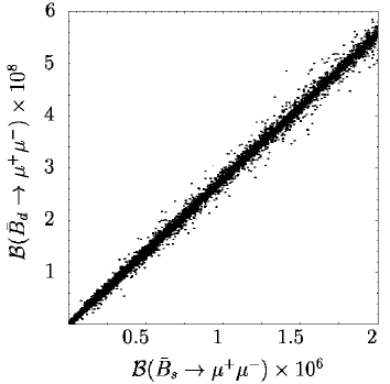
FIG. 3.: Predictions for the branching ratios ${\cal B}\,(\bar{B}_{d}\to\mu^{+}\mu^{-})$ vs. ${\cal B}\,(\bar{B}_{s}\to\mu^{+}\mu^{-})$ in scenario (B). The left plot shows the unconstrained parameter sets, with $R$ varying between $0.002\lesssim R\lesssim 0.115$. The right plot exhibits the results for the branching fractions, using the constrained parameter sets. In this case, $R$ varies between $0.026$ and $0.030$.

In Fig. 3, we have plotted ${\cal B}\,(\bar{B}_{d}\to\mu^{+}\mu^{-})$ versus ${\cal B}\,(\bar{B}_{s}\to\mu^{+}\mu^{-})$ for unconstrained and constrained parameter sets. In case of the former, the deviation of $R$ from $R_{\rm SM}$ can be one order of magnitude, with the range $0.002\lesssim R\lesssim 0.115$. Applying the constraints on the flavour-changing entries in the matrix $M^{2}_{\tilde{U}_{L}}$, as well as the bounds given in Eqs. (47)–(51), our numerical predictions for $R$ in scenario (B) are similar to those in scenario (A). In fact, $R$ varies between $0.026$ and $0.030$. It is important to note that the bounds on $\Delta^{ij}_{\tilde{U}_{L}}$ [17] severely constrain the additional chargino contributions in scenario (B) in contrast to scenario (A).

C Scenario (C)

We now repeat the analysis of the $\bar{B}_{d,s}\to\mu^{+}\mu^{-}$ decays within the framework of scenario (C). In this case, the matrix $M^{2}_{\tilde{U}_{L}}$ is diagonal,

$$M^{2}_{\tilde{U}_{L}}={\mathrm{diag}}(m^{2}_{\tilde{u}_{L}},m^{2}_{\tilde{c}_{L}},m^{2}_{\tilde{t}_{L}}),$$ (63)

with at least two different entries. According to the relation in Eq. (17), this implies that $M^{2}_{\tilde{D}_{L}}$ has non-diagonal entries, so that gluinos and neutralinos contribute to the $b\to ql^{+}l^{-}$ transition already at one-loop level. In this case, $M^{2}_{\tilde{D}_{L}}$ can be written as

$$M^{2}_{\tilde{D}_{L}}=V_{\text{CKM}}^{\dagger}M^{2}_{\tilde{U}_{L}}V_{\text{CKM}}=\left(\begin{array}[]{ccc}m^{2}_{\tilde{d}_{L}}&\Delta^{12}_{\tilde{D}_{L}}&\Delta^{13}_{\tilde{D}_{L}}\\ \Delta^{12*}_{\tilde{D}_{L}}&m^{2}_{\tilde{s}_{L}}&\Delta^{23}_{\tilde{D}_{L}}\\ \Delta^{13*}_{\tilde{D}_{L}}&\Delta^{23*}_{\tilde{D}_{L}}&m^{2}_{\tilde{b}_{L}}\end{array}\right),$$ (64)

where the flavour-changing off-diagonal entries are given by

$$\Delta^{12}_{\tilde{D}_{L}}=(m^{2}_{\tilde{u}_{L}}-m^{2}_{\tilde{c}_{L}})V_{us}V_{ud}^{*}+(m^{2}_{\tilde{t}_{L}}-m^{2}_{\tilde{c}_{L}})V_{ts}V_{td}^{*},$$ (66)

$$\Delta^{13}_{\tilde{D}_{L}}=(m^{2}_{\tilde{u}_{L}}-m^{2}_{\tilde{c}_{L}})V_{ub}V_{ud}^{*}+(m^{2}_{\tilde{t}_{L}}-m^{2}_{\tilde{c}_{L}})V_{tb}V_{td}^{*},$$ (67)

$$\Delta^{23}_{\tilde{D}_{L}}=(m^{2}_{\tilde{u}_{L}}-m^{2}_{\tilde{c}_{L}})V_{ub}V_{us}^{*}+(m^{2}_{\tilde{t}_{L}}-m^{2}_{\tilde{c}_{L}})V_{tb}V_{ts}^{*}.$$ (68)

As before, we take the constraints of Refs. [17, 28, 29] on these off-diagonal elements.

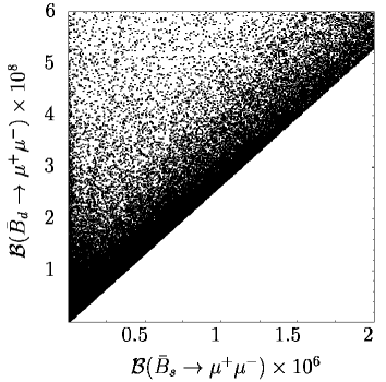
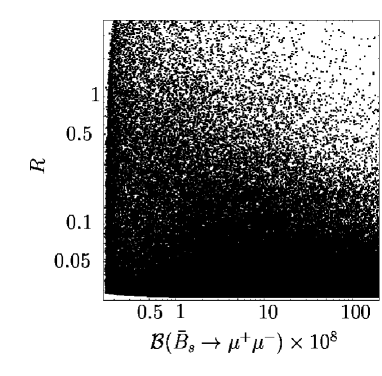
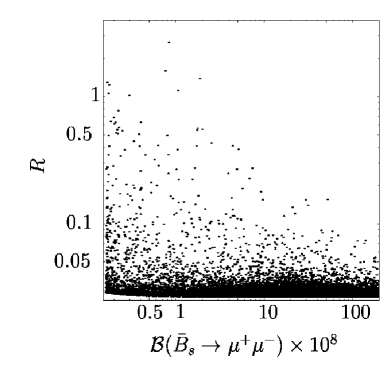
FIG. 4.: Predictions for the branching ratios ${\cal B}\,(\bar{B}_{d}\to\mu^{+}\mu^{-})$ vs. ${\cal B}\,(\bar{B}_{s}\to\mu^{+}\mu^{-})$ (upper plots) and $R$ vs. ${\cal B}\,(\bar{B}_{s}\to\mu^{+}\mu^{-})$ (lower plots) in scenario (C). The left plots show the unconstrained parameter sets, with $R$ varying between $0.026\lesssim R\lesssim 20.636$. The right plots exhibit the results for the branching fractions and their ratio $R$, using the constrained parameter sets. In this case, $R$ varies between $0.026$ and $2.863$.

The scatter plots in Fig. 4 exhibit an order-of-magnitude deviation from $R_{\rm SM}\approx 0.03$. In the unconstrained case (left plots) $R$ is predicted to be in the range $0.026\lesssim R\lesssim 20.636$, while for the constrained parameter sets (right plots) we find $0.026\lesssim R\lesssim 2.863$. A noticeable feature of scenario (C) is that there exists a lower bound on $R$, i.e. $R\gtrsim 0.95\,R_{\rm SM}$ (see upper plots of Fig. 4), which is due to the structure of the CKM matrix. We stress that this bound is valid only within scenario (C) and does not apply to scenario (B) or scenarios with new sources of flavour violation (see Sec. II).

FIG. 5.: ${\cal B}\,(\bar{B}_{d,s}\to\mu^{+}\mu^{-})$ as function of the charged Higgs boson mass, $M_{H}$, for $\tan\beta=50$ (left plot) and $\tan\beta=60$ (right plot), taking into account the experimental constraints on the rare $B$ decays and on the flavour-changing entries. The remaining parameters have been kept fixed, as described in the text.

In Fig. 5, the branching ratios of $\bar{B}_{d}\to\mu^{+}\mu^{-}$ and $\bar{B}_{s}\to\mu^{+}\mu^{-}$ are displayed as functions of the charged Higgs boson mass, $M_{H}$, for $\tan\beta$ equal to $50$ (left plot) and $60$ (right plot). The remaining parameters are given by

$$\mu=-800\ {\text{GeV}},\ M_{1}=500\ {\text{GeV}},\ M_{2}=200\ {\text{GeV}},\ M_{\tilde{g}}=250\ {\text{GeV}},$$ (70)

$$A_{U}=A_{D}={\rm diag}(100\ {\text{GeV}},\ 100\ {\text{GeV}},\ 75\ {\text{GeV}}),$$ (71)

$$M_{\tilde{U}_{R}}=M_{\tilde{D}_{R}}={\rm diag}(500\ {\text{GeV}},\ 500\ {\text{GeV}},\ 500\ {\text{GeV}}),$$ (72)

$$M_{\tilde{U}_{L}}={\rm diag}(460\ {\text{GeV}},\ 500\ {\text{GeV}},\ 517\ {\text{GeV}}).$$ (73)

Both plots are consistent with the constraints on rare $B$ decays in Eqs. (47)–(51), and with those on the flavour-changing entries $\Delta^{ij}_{\tilde{D}_{L}}$ [17]. Interestingly, in the left (right) plot, the ratio $R$ ranges between $0.15\lesssim R\lesssim 0.81$ ($0.44\lesssim R\lesssim 1.78$), while the magnitude of the individual branching fractions decreases drastically with increasing charged Higgs boson mass, $M_{H}$. Note that for small $M_{H}$ and $\tan\beta$ close to $60$ both branching ratios are in a region that can be probed experimentally, in Run II of the Fermilab Tevatron, BABAR and Belle. The large enhancement of $R$ is due to ${\text{Im}}\,[c_{S,P}^{\tilde{g}}(\bar{B}_{d}\to\mu^{+}\mu^{-})]$ being by an order-of-magnitude larger than ${\text{Im}}\,[c_{S,P}^{\tilde{g}}(\bar{B}_{s}\to\mu^{+}\mu^{-})]$ and a cancellation between the real parts of $c_{S,P}^{\tilde{\chi}^{\pm}}$ and $c_{S,P}^{\tilde{g}}$. As a consequence, the neutralino contributions to the scalar and pseudoscalar coefficients, although negligible compared to the corresponding contributions in the chargino and gluino sector, cannot be neglected in the $\bar{B}_{s}\to\mu^{+}\mu^{-}$ decay. The neutralinos contribute significantly to the ratio $R$; for illustration, the ratio $R\approx 0.94$ in the right plot ($\tan\beta=60$) at $M_{H}=130\ {\text{GeV}}$ increases to $R\approx 1.55$ after neglecting the contributions from neutralinos.

As already mentioned, we have found that the primed Wilson coefficients, $c_{S,P}^{\prime}$, are numerically suppressed. In fact, applying the mass insertion approximation as outlined in Appendix C, one can convince oneself that the enhancement factor $1/m_{q}$ (recall $q=s,d$) appearing in the scalar and pseudoscalar coefficients cancels out. Therefore, the primed Wilson coefficients are suppressed by a factor $m_{q}/m_{b}\ll 1$, compared to the unprimed coefficients.

VI Summary and conclusions

In the framework of the minimal supersymmetric extension of the SM with large $\tan\beta$, we have computed the gluino and neutralino exchange diagrams contributing to the purely leptonic decays $\bar{B}_{d,s}\to\mu^{+}\mu^{-}$. Together with our previous analysis [2], the present paper provides a complete study of the decays $\bar{B}_{d,s}\to\mu^{+}\mu^{-}$ at one-loop level in the MSSM with modified minimal flavour violation and large $\tan\beta$.

We have defined $\overline{\rm MFV}$ using symmetry arguments and have shown that $\overline{\rm MFV}$ is less restrictive than MFV, while the CKM matrix remains the only source of flavour violation. We have given a criterion for testing whether a theory belongs to the class of $\overline{\rm MFV}$. Within the MSSM we have investigated three scenarios that are possible within the context of $\overline{\rm MFV}$. In particular, we have studied the case where the gluino and neutralino exchange diagrams contribute besides $W^{\pm},H^{\pm},\tilde{\chi}^{\pm}$ [scenario (C)]. The neutralino Wilson coefficients are numerically smaller than those coming from the chargino and gluino contributions. However, we have found that in certain regions of the MSSM parameter space cancellations between the chargino and gluino coefficients occur, in which case the neutralino contributions become important. As a matter of fact, for the SUSY parameter sets examined, we found that a large value of $R\equiv{\cal B}\,(\bar{B}_{d}\to\mu^{+}\mu^{-})/{\cal B}\,(\bar{B}_{s}\to\mu^{+}\mu^{-})$ always involves such a cancellation.

Including current experimental data on rare $B$ decays, as well as on $K,B,D$ meson mixing, we found that in certain regions of the SUSY parameter space the branching ratios ${\cal B}\,(\bar{B}_{d}\to\mu^{+}\mu^{-})$ and ${\cal B}\,(\bar{B}_{s}\to\mu^{+}\mu^{-})$ can be up to the order of $10^{-7}$ and $10^{-6}$ respectively. Specifically, we showed that there exist regions in which the branching fractions of both decay modes are comparable in size, and may well be accessible to Run II of the Fermilab Tevatron.

We wish to stress that a measurement of the branching ratios ${\cal B}\,(\bar{B}_{d,s}\to\mu^{+}\mu^{-})$, or equivalently, a ratio $R$ of $O(1)$, does not necessarily imply the existence of new flavour violation outside the CKM matrix. Nevertheless, any observation of these decay modes in ongoing and forthcoming experiments would be an unambiguous signal of new physics.

A Auxiliary functions

The loop functions appearing in the formulae of Sec. IV are given by [2]

$$D_{2}(x,y)=\frac{x\ln x}{(1-x)(x-y)}+(x\leftrightarrow y),$$ (A1)

$$D_{3}(x)=\frac{x\ln x}{1-x}.$$ (A2)

B Mass matrices

1 Squark mass matrices

The squark mass-squared matrices given in Eq. (7) are diagonalized according to

$$\Gamma^{U}{\cal M}_{U}^{2}\Gamma^{U{\dagger}}={\mathrm{diag}}(m_{\tilde{u}_{1}}^{2},\dots,m_{\tilde{u}_{6}}^{2}),\quad\Gamma^{D}{\cal M}_{D}^{2}\Gamma^{D{\dagger}}={\mathrm{diag}}(m_{\tilde{d}_{1}}^{2},\dots,m_{\tilde{d}_{6}}^{2}).$$ (B1)

It is convenient to split the $6\times 6$ squark mixing matrices, $\Gamma^{U,D}$, into two $6\times 3$ submatrices:

$$(\Gamma^{Q})_{ai}=(\Gamma^{Q_{L}})_{ai},\quad(\Gamma^{Q})_{a,i+3}=(\Gamma^{Q_{R}})_{ai},\quad Q=U,D,$$ (B2)

where $a=1,\dots,6$ and $i=1,2,3$.

2 Neutralino mass matrix

The neutralino mass matrix has the structure [31]

$${\cal M}_{\tilde{\chi}^{0}}=\left(\begin{array}[]{cccc}M_{1}&0&-M_{Z}\sin\theta_{W}\cos\beta&M_{Z}\sin\theta_{W}\sin\beta\\ 0&M_{2}&M_{Z}\cos\theta_{W}\cos\beta&-M_{Z}\cos\theta_{W}\sin\beta\\ -M_{Z}\sin\theta_{W}\cos\beta&M_{Z}\cos\theta_{W}\cos\beta&0&-\mu\\ M_{Z}\sin\theta_{W}\sin\beta&-M_{Z}\cos\theta_{W}\sin\beta&-\mu&0\end{array}\right),$$ (B3)

which is diagonalized by a unitary matrix $N$ such that

$$N^{\ast}{\cal M}_{\tilde{\chi}^{0}}N^{{\dagger}}={\mathrm{diag}}(M_{\tilde{\chi}^{0}_{1}},M_{\tilde{\chi}^{0}_{2}},M_{\tilde{\chi}^{0}_{3}},M_{\tilde{\chi}^{0}_{4}}).$$ (B4)

C Perturbative diagonalization of ${\cal M}_{D}^{2}$

Within the framework of scenario (C), all flavour-changing interactions and CP violation are due exclusively to the CKM matrix. In this case, the matrices ${\cal M}^{2}_{D_{LR}}$ and ${\cal M}^{2}_{D_{RR}}$ in Eq. (7) are diagonal and real whereas ${\cal M}^{2}_{D_{LL}}$ contains complex off-diagonal entries [cf. Eq. (64)]. In order to diagonalize the down squark mass-squared matrix ${\cal M}^{2}_{D}$ perturbatively, we rewrite it as

$${\cal M}_{D}^{2}=\widetilde{{\cal M}}_{D}^{2}+\widetilde{\Delta}_{D}=\Bigg{(}\begin{array}[]{cc}\widetilde{{\cal M}}^{2}_{D_{LL}}&{\cal M}^{2}_{D_{LR}}\\ {\cal M}^{2}_{D_{LR}}&{\cal M}^{2}_{D_{RR}}\end{array}\Bigg{)}+\Bigg{(}\begin{array}[]{cc}\Delta_{D_{LL}}&0\\ 0&0\end{array}\Bigg{)},$$ (C1)

where $\widetilde{{\cal M}}^{2}_{D_{LL}}$ (${\Delta}_{D_{LL}}$) contains the diagonal (off-diagonal) elements of ${\cal M}^{2}_{D_{LL}}$. We remark parenthetically that for large values of $\tan\beta$ the LR elements in ${\cal M}^{2}_{D}$ cannot in general be treated as small perturbations. [This is the reason for choosing the decomposition of ${\cal M}^{2}_{D}$ given in Eq. (C1).]

Writing $\Gamma^{D}$ as a product of two unitary matrices, $\Gamma^{D}\equiv XY$, we have

$$({\cal M}_{D}^{2})_{\mathrm{diag}}=\Gamma^{D}{\cal M}_{D}^{2}\Gamma^{D{\dagger}}=X\left\{D+\Delta_{D}\right\}X^{\dagger},$$ (C2)

where $D=Y\widetilde{{\cal M}}_{D}^{2}Y^{\dagger}\equiv{\mathrm{diag}}(D_{1},\dots,D_{6})$ and $\Delta_{D}=Y\widetilde{\Delta}_{D}Y^{\dagger}$. Then, if $|(\Delta_{D})_{ij}|\ll D_{a}$, we can make the ansatz

$$X = \openone+\delta X^{(1)}+\delta X^{(2)}+\cdots,$$ (C3)

$$({\cal M}_{D}^{2})_{\mathrm{diag}} = D+\delta D^{(1)}+\delta D^{(2)}+\cdots$$ (C4)

to solve Eq. (C2) perturbatively in terms of $\Delta_{D}$. As a result, we obtain

$$\Gamma_{ac}^{D{\dagger}}f(m^{2}_{\tilde{d}_{c}})\Gamma^{D}_{cb} = Y_{ac}^{\dagger}f(D_{c})Y_{cb}+Y_{ac}^{\dagger}\Delta_{cd}f_{1}(D_{c},D_{d})Y_{db}$$ (C5)

$$+ Y_{ac}^{\dagger}\Delta_{ce}\Delta_{ed}f_{2}(D_{c},D_{d},D_{e})Y_{db}+\cdots,$$ (C6)

where $f$ denotes an arbitrary loop function, and

$$f_{1}(x,y)=\frac{f(x)-f(y)}{x-y},\quad f_{2}(x,y,z)=\frac{f_{1}(x,z)-f_{1}(y,z)}{x-y},$$ (C7)

for $x\neq y\wedge x\neq z\wedge y\neq z$. In all other cases the corresponding limit of the functions $f_{1,2}$ has to be taken. Setting $Y\equiv\openone$ in Eq. (C5) reproduces the result given in Refs. [32].

REFERENCES

- [1] A. J. Buras, in Flavour Dynamics: CP Violation and Rare Decays, Lectures given at International School of Subnuclear Physics, Erice, Italy, 2000, hep-ph/0101336.
- [2] C. Bobeth, T. Ewerth, F. Krüger, and J. Urban, Phys. Rev. D 64, 074014 (2001).
- [3] UKQCD Collaboration, K. C. Bowler et al., Nucl. Phys. B619, 507 (2001); C. Bernard, Nucl. Phys. B (Proc. Suppl.) 94, 159 (2001); C. T. Sachrajda, Nucl. Instrum. Meth. A 462, 23 (2001); S. Ryan, Nucl. Phys. B (Proc. Suppl.) 106, 86 (2002).
- [4] Belle Collaboration, Report No. BELLE-CONF-0127 (unpublished); CDF Collaboration, F. Abe et al., Phys. Rev. D 57, 3811 (1998).
- [5] C.-S. Huang and Q.-S. Yan, Phys. Lett. B 442, 209 (1998); C.-S. Huang, W. Liao, and Q.-S. Yan, Phys. Rev. D 59, 011701 (1999); K. S. Babu and C. Kolda, Phys. Rev. Lett. 84, 228 (2000); G. Isidori and A. Retico, J. High Energy Phys. 11, 001 (2001).
- [6] P. H. Chankowski and Ł. Sławianowska, Phys. Rev. D 63, 054012 (2001).
- [7] C.-S. Huang, W. Liao, Q.-S. Yan, and S.-H. Zhu, Phys. Rev. D 63, 114021 (2001); ibid. 64, 059902(E) (2001).
- [8] A. J. Buras, P. H. Chankowski, J. Rosiek and Ł. Sławianowska, Nucl. Phys. B619, 434 (2001).
- [9] A. J. Buras, P. H. Chankowski, J. Rosiek and Ł. Sławianowska, hep-ph/0207241.
- [10] A. Dedes, H. K. Dreiner, and U. Nierste, Phys. Rev. Lett. 87, 251804 (2001).
- [11] R. Arnowitt, B. Dutta, T. Kamon, and M. Tanaka, Phys. Lett. B 538, 121 (2002); D. A. Demir, K. A. Olive, and M. B. Voloshin, hep-ph/0204119.
- [12] S. Bergmann and G. Perez, Phys. Rev. D 64, 115009 (2001); A. J. Buras and R. Fleischer, Phys. Rev. D 64, 115010 (2001); S. Laplace, Z. Ligeti, Y. Nir and G. Perez, Phys. Rev. D 65, 094040 (2002); P. H. Chankowski and J. Rosiek, hep-ph/0207242.
- [13] A. J. Buras, P. Gambino, M. Gorbahn, S. Jäger and L. Silvestrini, Phys. Lett. B 500, 161 (2001).
- [14] A. Ali and D. London, Eur. Phys. J. C 9, 687 (1999).
- [15] M. Ciuchini, G. Degrassi, P. Gambino and G. F. Giudice, Nucl. Phys. B534, 3 (1998); A. J. Buras, P. Gambino, M. Gorbahn, S. Jäger and L. Silvestrini, Nucl. Phys. B592, 55 (2001).
- [16] G. D’Ambrosio, G. F. Giudice, G. Isidori and A. Strumia, hep-ph/0207036.
- [17] M. Misiak, S. Pokorski, and J. Rosiek, in Heavy Flavours II, edited by A. J. Buras and M. Lindner (World Scientific, Singapore, 1998), p. 795, hep-ph/9703442.
- [18] M. Jamin and B. O. Lange, Phys. Rev. D 65, 056005 (2002).
- [19] J. Rosiek, Phys. Rev. D 41, 3464 (1990); hep-ph/9511250.
- [20] Z. Xiong and J. M. Yang, Nucl. Phys. B628, 193 (2002).
- [21] Z. Xiong (private communication).
- [22] A. Ali, E. Lunghi, C. Greub, and G. Hiller, hep-ph/0112300.
- [23] Belle Collaboration, K. Abe et al., hep-ex/0107072; see also BABAR Collaboration, B. Aubert et al., Phys. Rev. Lett. 88, 241801 (2002).
- [24] Belle Collaboration, K. Abe et al., Phys. Rev. Lett. 88, 021801 (2002).
- [25] ALEPH Collaboration, R. Barate et al., Phys. Lett. B 429, 169 (1998); CLEO Collaboration, S. Chen et al., Phys. Rev. Lett. 87, 251807 (2001); Belle Collaboration, K. Abe et al., Phys. Lett. B 511, 151 (2001).
- [26] Particle Data Group, D. E. Groom et al., Eur. Phys. J. C 15, 1 (2000).
- [27] C. Bobeth, A. J. Buras, F. Krüger, and J. Urban, Nucl. Phys. B630, 87 (2002).
- [28] T. Besmer, C. Greub, and T. Hurth, Nucl. Phys. B609, 359 (2001).
- [29] See also F. Gabbiani, E. Gabrielli, A. Masiero, and L. Silvestrini, Nucl. Phys. B477, 321 (1996); D. Chang, W. F. Chang, W. Y. Keung, N. Sinha, and R. Sinha, Phys. Rev. D 65, 055010 (2002).
- [30] G. Raz, hep-ph/0205310; J. Rosiek (private communication).
- [31] H. E. Haber and G. L. Kane, Phys. Rep. 117, 75 (1985).
- [32] A. J. Buras, A. Romanino, and L. Silvestrini, Nucl. Phys. B520, 3 (1998); G. Colangelo and G. Isidori, J. High Energy Phys. 09, 009 (1998).