GR@PPA_4b: A Four Bottom Quark Production Event Generator for $pp$/$p\bar{p}$ Collisions

Abstract

We have developed an event generator, named GR@PPA_4b, for the four bottom quark ($b\bar{b}b\bar{b}$) production processes at $pp$ and $p\bar{p}$ collisions. The program implements all of the possible processes at the tree level within the framework of the Standard Model. Users can generate events from the Higgs boson and $\gamma/Z$ mediated processes, as well as those from pure QCD interactions. The integration and the event generation are performed within the newly developed GR@PPA framework, an extension of the GRACE automatic event-generator generation system to hadron collisions. This program is so designed that it can be embedded in a general-purpose event generator PYTHIA version 6.1. PYTHIA adds the initial- and final-state parton showers and simulates the hadronization and decays to make generated events realistic. It should be emphasized that a huge number of diagrams and complicated four-body kinematics are dealt with strictly in GR@PPA_4b. This program will be useful for studies of Higgs boson productions, especially those in extended models where the Yukawa coupling to $b$ quarks is greatly enhanced.

The source code is located in http://atlas.kek.jp/physics/nlo-wg/index.html.

PROGRAM SUMMARY

1 Introduction

Despite the remarkable success of the Standard Model (SM) in high energy physics during the recent decades, nothing is known about the source of its fundamental theoretical basis, the Higgs mechanism, because the Higgs bosons, the remnants of this mechanism, remain undiscovered. The search for the Higgs bosons is thus considered to be the most important subject in the Tevatron Run II [1] and forthcoming LHC [2] experiments.

The properties of the Higgs bosons, thus promising search channels, depend on the underlying theory. The minimal supersymmetric extension of the Standard Model (MSSM) [3], which is considered to be a promising theory to solve difficulties in the SM, requires the existence of three neutral Higgs bosons. Among them, the CP-odd one and, in many cases, one of the two CP-even ones, have appreciably large couplings to the bottom quark over a wide parameter range (large $\tan\beta$ regions). The production associated with a bottom quark pair is a promising search channel in this case.

These Higgs bosons with large couplings to the bottom quark predominantly decay to a bottom quark pair. Therefore, this process can be experimentally tagged as four bottom-quark events, and the Higgs boson production can be identified by a resonant enhancement in the invariant mass spectrum of two bottom quarks. In spite of such a clear signature, a discovery in this way is not trivial because of the presence of the huge QCD background [4, 5]. Actually, a previous study for LHC [6] showed a discouraging result. Because only crude estimates based on many approximations have been available for the background processes, the prospects are still quite ambiguous.

In order to provide more reliable tools for this kind of studies, we have developed a Monte Carlo event generator of four bottom-quark productions from $pp$ and $p\bar{p}$ collisions. The program, named GR@PPA_4b, calculates the cross section and generates realistic (unweighted) events, based on a complete tree-level calculation of all possible processes within the Standard Model, including QCD processes as well as the Higgs boson and $\gamma$/$Z$ mediated processes. The results can be applied to MSSM cases by changing the normalization for the Higgs boson-mediated processes according to the change of the coupling strength.

The core part of the program, describing parton-level hard interactions, was generated by using an automatic calculation system, called GRACE [7]. Because the GRACE system has been developed mainly aiming at applications to lepton collisions, generated codes are not directly applicable to hadron-collision interactions. We have developed an extended framework, called GR@PPA (GRACE at PP/Anti-p), to implement those features specific to hadron collisions [8]. The primary function of GR@PPA is to determine the initial-state partons, $i.e.$ their flavors and momenta, by referring to a parton distribution function (PDF). Since the GR@PPA framework is not process-specific, it can be applied to any other processes in hadron collisions.

Based on the GRACE output codes, GR@PPA calculates the cross section and generates unweighted parton-level events using BASES/SPRING [9] included in the GRACE system. The GR@PPA framework also includes an interface to a general-purpose event generator, PYTHIA version 6.1 [10]. Using this interface, the GR@PPA program can be totally embedded in a PYTHIA program. The generated parton-level event information, including the color flow, is automatically passed to PYTHIA. The initial- and final-state radiation, hadronization and decays can be implemented by PYTHIA, to make the generated events realistic.

This paper is organized as follows: the GR@PPA extension of the GRACE system is described in Section 2. The features of GR@PPA_4b are specified in Section 3. All details about running the program are given there. Some physical results and program performances are presented in Section 4. A summary is given in Section 5. Typical Feynman diagrams of the processes implemented in the program are shown in the appendix.

2 GR@PPA

2.1 Extension of GRACE to $pp$/$p\bar{p}$ collisions

Cross sections with a hard interaction in $pp$/$p\bar{p}$ collisions can be described as

$$\sigma=\sum_{i,j,F}\int dx_{1}\int dx_{2}\int d\hat{\Phi}_{F}f^{1}_{i}(x_{1},Q^{2})f^{2}_{j}(x_{2},Q^{2}){d\hat{\sigma}_{ij\rightarrow F}(\hat{s})\over d\hat{\Phi}_{F}},$$ (1)

where $f^{a}_{i}(x_{a},Q^{2})$ is a PDF of the hadron $a$ ($p$ or $\bar{p}$), which gives the probability to find the parton $i$ with an energy fraction $x_{a}$ at a probing virtuality of $Q^{2}$. The differential cross section $d\hat{\sigma}_{ij\rightarrow F}(\hat{s})/d\hat{\Phi}_{F}$ describes the parton-level hard interaction producing the final-state $F$ from a collision of partons, $i$ and $j$, where $\hat{s}$ is the square of the total initial 4-momentum. The sum is taken over all relevant combinations of $i$, $j$ and $F$. Note that in hadron interactions a certain ”process” of interest may contain some incoherent subprocesses having different final states, as well as those having different combinations of the initial-state partons. For example, the ”two-jet” production process includes all $q\bar{q^{\prime}}$, $qg$($\bar{q}g$) and $gg$ production processes.

The original GRACE system assumes that both the initial and final states are well-defined. Hence, it can be applied to evaluating $d\hat{\sigma}_{ij\rightarrow F}(\hat{s})/d\hat{\Phi}_{F}$ and its integration over the final-state phase space $\hat{\Phi}_{F}$ only. An adequate extension is necessary to take into account the variation of the initial state both in parton species and their momenta, in order to make the GRACE system applicable to hadron collisions.

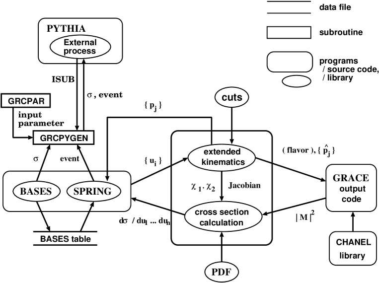
Figure 1: Picture showing the structure of GR@PPA. The data flow is indicated schematically. The main building blocks of the GRACE-based event generator are BASES/SPRING and ”GRACE output codes”. The interface between them has been extended for $pp$ and $p\bar{p}$ collisions. A set of random numbers {$u_{i}$} given by BASES/SPRING includes two numbers for defining the initial state ($x_{1}$ and $x_{2}$), in addition to those for defining the final state. The cross section is calculated from the matrix element returned from the ”GRACE output codes”, by referring to a PDF using $x_{1}$ and $x_{2}$. Some phase-space cuts are applied by limiting the range of kinematical variables, or by setting the cross section to zero after the kinematical variables are determined. In some cases, several subprocesses are combined to a single subprocess by adding one more random number for defining the quark flavor. This system is interfaced to PYTHIA 6.1 through grcpygen and PYUPEV.

The structure of the GR@PPA system is schematically drawn in Fig. 1. The basic elements of the system, which are the same as the original GRACE system, are the ”GRACE output code” and BASES/SPRING. The ”GRACE output code” is a set of FORTRAN codes for calculating the matrix element of a specified process, according to a set of kinematical variables specifying a phase-space point. The codes can be automatically generated using a utility included in the GRACE system. The codes for four-$b$ production processes have been generated by the authors and included in the GR@PPA_4b distribution.

BASES/SPRING is a multi-dimensional general-purpose Monte Carlo integration and event-generation program set. It generates a set of random numbers to give them to an external function. Using the returned answer, BASES performs an integration and SPRING generates ”events” by means of a hit/miss method. The most remarkable feature of the BASES/SPRING system is the utilization of a multi-dimensional grid method for the random number generation. BASES optimizes the grid setting by an iteration to maximize the efficiency of the integration and the event generation. The optimized setting is stored in an external file (BASES table) to be used later in the event generation by SPRING.

The remaining task required to GRACE users is to prepare the interface between BASES/SPRING and the ”GRACE output code”. The interface has to convert the random numbers given by BASES/SPRING to a set of kinematical variables necessary for the matrix element calculation (”kinematics”), and to convert the returned matrix element to the differential cross section. Singular structures such as the $1/k$ singularity of the photon/gluon radiation and Breit-Wigner resonance structures, has to be taken into account in the conversion to the kinematical variables, using their well-known asymptotic forms. Although the grid method of BASES/SPRING is very flexible and practically very powerful, by itself, it is not capable of dealing with these singularities without any care.

An extension has been made in the interface between BASES/SPRING and the GRACE output code. We require BASES/SPRING to provide two additional random numbers, in order to determine the initial-state variables, $x_{1}$ and $x_{2}$. Due to a $1/x$ asymptotic behavior of the structure functions, it is convenient for Monte Carlo integration and event generation to rewrite Eq. (1) as

$$\sigma=\sum_{i,j,F}\int\frac{d\tau}{\tau}\int dy\int d\hat{\Phi}_{F}x_{1}f^{1}_{i}(x_{1},Q^{2})x_{2}f^{2}_{j}(x_{2},Q^{2}){d\hat{\sigma}_{ij\rightarrow F}(\hat{s})\over d\hat{\Phi}_{F}},$$ (2)

where

$$\tau=x_{1}x_{2}\;,\quad\quad y=\frac{1}{2}\ln\frac{x_{1}}{x_{2}}.$$ (3)

In GR@PPA, the added two random numbers are converted to $\tau$ and $y$, while taking into account the asymptotic $1/\tau$ behavior for $\tau$, and assuming a flat probability distribution for $y$. The variable $\tau$ determines the center-of-mass (cm) energy of the hard interaction, since $\hat{s}$ $=$ $\tau s$. The variables $x_{1}$ and $x_{2}$ are derived using Eq. (3) in order to refer to PDFs in the conversion of the returned matrix element to the differential cross section, as shown in Fig. 1. The interface finally returns the calculated differential cross section to BASES/SPRING, and at the same time converts the kinematical variables in the cm frame to ones in the laboratory frame, by applying a Lorentz boost determined by $y$.

As already mentioned, a ”process” of interest is usually composed of several incoherent subprocesses in hadron interactions. However, the present version of BASES/SPRING can treat only one subprocess at the same time. This does not matter in BASES. It is sufficient to do the integration and the grid optimization sequentially for these subprocesses, one after the other. On the other hand, this is a serious limitation in event generation by SPRING, because we frequently want to generate events of different subprocesses in a random order.

We applied a slight modification to SPRING to overcome this difficulty. The ”BASES table” is prepared for every subprocess by running BASES sequentially over the subprocesses. The modified SPRING works as follows: when SPRING is called at the first time, all relevant ”BASES tables” are read into a tentative memory area. The main ”BASES table” to be used for random-number generation is replaced in each event, by copying an appropriate one from the tentative memory. This method works well because entire information specific to subprocesses, such as the optimized grid information and the cross section information, is recorded in the ”BASES table”.

Although we successfully extended the BASES/SPRING to multiple subprocesses, the number of subprocesses is desired to be as small as possible because we have to prepare not only the ”BASES table”, but also the ”GRACE output codes” for every subprocess. In many cases, the difference between the subprocesses is the difference in the quark combination in the initial and/or final states only. The matrix element of these subprocesses is frequently identical, or the difference is only in a few coupling parameters and/or masses. In such cases, it is convenient to add one more integration/differentiation variable to replace the summation in Eqs. (1) and (2) with an integration. As a result, these subprocesses can share an identical ”GRACE output code” and can be treated as a single subprocess by BASES/SPRING. This extension is implemented in GR@PPA_4b for $q\bar{q}\rightarrow b\bar{b}b\bar{b}$ subprocesses.

2.2 Interface to PYTHIA

As shown in Fig. 1, GR@PPA includes an interface to a general-purpose event generator PYTHIA version 6.1. Using a facility in PYTHIA, we can add the effect of initial- and final-state parton showers to the generated events. This effect emerges as a finite overall $p_{T}$ of the hard interaction system and finite underlying activities. Furthermore, if we activate the hadronization and decay, we can obtain realistic events which can be passed to detector simulators.

We use the subroutine PYUPEV, prepared by PYTHIA to deal with external generators, as the interface in the PYTHIA side. The prepared PYUPEV simply calls the GR@PPA steering routine grcpygen. The subroutine grcpygen controls BASES/SPRING and, as a result, controls all GR@PPA routines.

When PYUPEV is used to generate events of user-defined processes, PYTHIA requires users to specify the estimated maximum cross section SIGMAX for each process in the initialization stage by using the subroutine PYUPIN. PYUPEV is required to return the normalized cross section SIGEV for each event. The SIGEV is so defined that the average should become the total cross section. The ratio SIGEV/SIGMAX is the weight of this event. PYTHIA determines ”accept or reject” of the event using this weight.

The subroutine grcpygen calls BASES or SPRING according to the mode selection determined by an input argument. In GR@PPA, users must call grcpygen in the initialization stage before calling the PYTHIA initialization by PYINIT, with the mode selection for calling BASES to evaluate the total cross section. In this call, grcpygen internally calls PYUPIN by setting the argument SIGMAX equal to the evaluated total cross section. In the event generation cycle, PYUPEV calls grcpygen with the mode selection for calling SPRING. Since the event generation is totally controlled by SPRING in GR@PPA, the rejection in PYTHIA must be deactivated. For this purpose, the returned argument of grcpygen, which is directly passed to the argument SIGEV of PYUPEV, is always set equal to the total cross section evaluated by BASES.

The calling sequence of grcpygen is as follows:

call grcpygen(beams, ISUB, mode, sigma),

where the input arguments are

beams (CHARACTER)	: ’PP’ for $pp$ collisions and ’PAP’ for $p\bar{p}$ collisions
ISUB (INTEGER)	: subprocess number
mode (INTEGER)	: = 1 for calling BASES, and 0 for calling SPRING,

and the output is

sigma (REAL*8) : integrated cross section.

The argument beams is a dummy when mode = 0. PYTHIA requires users to assign a unique subprocess number ISUB to every user-defined subprocess. The output sigma is always equal to the integrated cross section of the subprocess specified by ISUB.

The most important task of grcpygen in the event generation cycle is to pass the event information determined in GR@PPA to PYTHIA. The interfacing rules are all specified by PYTHIA. The information concerning the parton species and momenta, which has been determined in the ”kinematics” routines and passed through the user interface routine of SPRING, is copied to the arrays in the common PYUPPR. The color flow information, which is necessary to perform hadronization, is also recorded, based on the information from SPRING [12].

3 GR@PPA_4b

3.1 Subprocesses

Based on the GR@PPA framework, we have developed an event generator, called GR@PPA_4b, for the production of four bottom quarks ($b\bar{b}b\bar{b}$) in $pp$ and $p\bar{p}$ collisions. The calculations are all done within the framework of the minimal Standard Model. We divide the process into eight subprocesses according to the difference in the initial state and the order of the couplings, as listed in Table 1. The subprocesses are listed in the order of the subprocess number (ISUB). We assigned those numbers reserved in PYTHIA for user-defined processes. The number of included Feynman diagrams is also listed in the table for each subprocess. We can see that a large number of diagrams which are hard to manage manually are included.

In GR@PPA_4b we do not account for bottom quarks in the initial state; namely, only the lighter quark ($u$, $d$, $s$ and $c$) pairs, as well as the gluon pairs, are counted as the initial state. Since the lighter quarks do not appear in the final state, the functional form of the matrix element is identical for all quark-initiated subprocesses. We treat these subprocesses as a single subprocess, by adding one variable for the choice of the initial-state quark flavor, as explained in a previous section. We generated the ”GRACE output code” for each of these combined subprocesses. Note that the interference between those diagrams belonging to different subprocesses are ignored in GR@PPA_4b.

We include all order-four tree level interactions within the Standard Model in this generator. Typical diagrams are shown in Appendix A. The symbol $y_{b}$ in Table 1 represents the Yukawa coupling between the Higgs boson and the bottom quark. We ignore the Yukawa couplings of lighter quarks. Those subprocesses including $y_{b}^{2}$ are composed of diagrams including a bottom-quark pair production mediated by the Higgs boson. Namely, they are the ”signal” processes according to our present interest.

The strong and electroweak couplings are symbolically represented by $\alpha_{s}$ and $\alpha_{em}$, respectively. The subprocesses classified as $\alpha_{s}^{2}\alpha_{em}^{2}$ include irreducible ”$Z^{0}$ background”. Those classified as $\alpha_{s}^{4}$ are the non-resonant but most serious ”QCD backgrounds”. The contribution of the subprocesses classified as $\alpha_{em}^{2}y_{b}^{2}$ and $\alpha_{em}^{4}$ is expected to be small but included for the completeness.

3.2 Distribution package

The distribution package is arranged for the use on Unix systems. However, since the structure is rather simple, we expect that the program can be compiled and executed on other platforms without serious difficulties. The package is composed of the following files and directories:

Makefile	:	the Makefile for the setup,
		Makefile.aix, Makefile.linux and Makefile.solaris are
		example Makefiles for IBM-AIX, Linux and Solaris, respectively,
README	:	a file describing how to set up the programs,
VERSION-1.0	:	a note for this version,
400/ - 407/	:	”GRACE output codes”; the directory name corresponds to
		the subprocess number,
basesv5.1/	:	BASES/SPRING (version 5.1) source codes,
chanel/	:	CHANEL source codes,
grckinem/	:	source codes of kinematics,
example/	:	source codes of example programs,
inc/	:	INCLUDE files,
lib/	:	the directory to store object libraries; initially empty.

Users have to edit the file Makefile to specify an appropriate compiler and associated compile options, as well as the paths to the GR@PPA_4b directory, and PYTHIA and CERNLIB libraries. Those parts to be edited can be found at the top of the Makefile. We prepared examples for IBM-AIX, Linux and Solaris systems. All library routines are compiled and combined to object libraries if users execute the command make from the GR@PPA_4b top directory. The object libraries are then moved to the directory lib/ if the command make install is executed. The Makefiles of example programs in example/ are set up by executing make example.

3.3 Dependencies on PYTHIA

GR@PPA_4b internally uses some utility programs provided by PYTHIA. The functions PYALEM and PYALPS are used to determine the $Q^{2}$-dependent coupling strengths of QED and QCD in the matrix element calculation. Since the $Q^{2}$ is given to these functions as an argument, their behaviors are basically controlled by GR@PPA_4b routines. However, they require additional parameters to define the running. Users are required to set relevant control parameters, such as PARU(112) before calling any initialization routines.

In addition, GR@PPA_4b uses the PYTHIA function PYPDFU for referring to PYTHIA built-in PDFs. Users have to make a choice of PDF by setting the parameter MSTP(51). The phase-space cuts defined by the PYTHIA parameters CKIN(1, 2, 7, 8, 21 - 28) are also applied in GR@PPA_4b if they are specified. These cuts are referred to in the definition of the ”kinematics”; namely, they limit the range of kinematical variables of the final state.

3.4 Initialization and customization

Although the execution of GR@PPA is controlled by the subroutine grcpygen, the detailed behavior depends on some parameters in common blocks and conditions defined in some subprograms. Users can change those details by changing appropriate parameters and subprograms described in the following.

The parameter that is necessary to be given by users is grcecm, which specifies the cm energy of the beam collision in GeV. Optionally, users can define some phase-space cuts in the laboratory frame: gptcut, getacut and grconcut. These parameters define the minimum $p_{T}$ in GeV, the largest pseudorapidity in the absolute value and the minimum separation in $\Delta R$, respectively, to be required to all produced $b$ quarks. The separation ($\Delta R$) is defined for every pair of $b$ quarks as

$$\Delta R=\sqrt{\Delta\phi^{2}+\Delta\eta^{2}},$$ (4)

where $\Delta\phi$ and $\Delta\eta$ are the separation in the azimuthal angle and the pseudorapidity, respectively. These parameters are accessible if the file grchad.inc in the directory inc/ is included. These cuts are applied after the kinematical variables of an event are determined. In addition, users can define their own cuts by editting the subroutine grcusrcut, in which 4-momenta of all partons are provided through a common block. Note that, since these cuts are applied during the event generation in SPRING, they are smeared by later simulations in PYTHIA.

Most of the conditions of GR@PPA_4b are defined in the subroutine grcpar, included in the file grcpar.F in example/pyth/. Those parameters which users are allowed to change are listed in Table 2. Users can choose different conditions for different subprocesses. The integer variable ibswrt controls whether BASES should be called in the initialization or not. The task of BASES is to optimize the integration grids and, after that, store the optimized results in a ”BASES table”. The execution of BASES consumes much CPU time because a precise evaluation is necessary for an efficient event generation by SPRING. It is not necessary to repeat the execution for identical conditions. A previously optimized result (”BASES table”) is reused if ibswrt = 1. It should be noted that, once the CKIN cuts and/or cuts by gptcut, getacut, grconcut, and user defineded-cuts are changed, the ”condition” is no longer identical and BASES has to be re-executed. Of course, users have to set ibswrt = 0 if they change other fundamental parameters, such as the cm energy, the incident beams and PDF described before, as well as the energy scales and the particle masses described below.

The variable icoup determines the energy scale ($Q^{2}$) for calculating the coupling strengths, $\alpha_{em}$ and $\alpha_{s}$, in the matrix element calculation (renormalization scale). Namely, the determined $Q^{2}$ is passed to PYALEM and PYALPS. The selectable choices are listed in Table 2. The variable ifact determines $Q^{2}$ for PDF (factorization scale). The definition is the same as icoup. The same choice as icoup is taken if ifact is not explicitly given. As an option, users can apply their own definitions of these energy scales, by setting icoup = 6 and/or ifact = 6 and editing the subroutine grcusrsetq. An example is attached to grcpar.F.

The parameter ncall specifies the number of sampling points in each step of the iterative grid optimization in BASES. The larger this number is, the better the conversion would be. However, it takes longer in the CPU time. The optimized values are preset in grcpar.F. The character variable grcfile gives the “BASES table” file name. A new file must be specified if ibswrt = 0, while an existing file must be specified if ibswrt = 1.

The particle masses, decay widths and couplings to be used in the matrix element calculation are defined in the subroutine setmas included in grcpar.F. The mass and the total decay width of the Higgs boson can be manually controlled. GR@PPA_4b does not give any constraint to these parameters. For some heavy particle masses and widths, the same values are set to the corresponding PYTHIA parameters in order to preserve the consistency.

PYTHIA requires PYUPEV users to combine the final-state partons into pairs and to give the energy scale of the final-state parton shower for each pair. The definition is rather trivial for those subprocesses in which at least one of the $b\bar{b}$ pairs is produced via a color-singlet particle production, $\gamma/Z$ and the Higgs boson. On the other hand, there is not any established guiding principle for pure QCD subprocesses. We give a definition based on the color flow in these cases. The energy scale is set equal to the invariant mass of each color-connected pair. Users can try their own definitions by editing the subroutine grcxxxdetc included in the file spxxxdetc.F in subprocess directories, where xxx denotes an ISUB number. The energy scale of the initial-state parton shower in PYHTIA is taken to be equal to the factorization scale for PDF, as the default. Users can also change this definition in the above subroutine if they want.

3.5 Sample program

A sample program sample_pyth.F is provided in the subdirectory example/pyth/. Execution of the command make example from the GR@PPA_4b top directory sets up the Makefile for this program.

The program, first of all, sets the initialization parameters described in the last section, together with some additional PYTHIA parameters. After that, it calls grcpygen for the initialization. BASES optimizes the integration grids and evaluates the total cross section here if ibswrt = 0. Note that grcpygen has to be called for every subprocess that users want to activate.

The initialization of PYTHIA by PYINIT is done after that. It is necessary to set MSUB parameters before the initialization, in order to activate the subprocesses. The parameter MSEL should be set to zero.

An event generation loop follows the initialization part. A call to PYEVNT automatically results in a call to grcpygen through PYUPEV. The source code of PYUPEV, dedicated to the use in GR@PPA_4b, is attached to the bottom of this sample program. The generated event information is returned in the common PYJETS. This sample program outputs the information of the produced four $b$ quarks as an Ntuple file. Users can obtain some histograms by executing the sample macro sample.kumac in the environment of PAW. Refer to the PAW manual [13] for the usage of Ntuple and PAW.

In the output of GR@PPA_4b, users should pay appropriate attention to the print out from BASES, especially when they apply tight cuts. Since each subprocess is composed of many coherent diagrams, it is not practicable to take all singularities into account in the ”kinematics” definitions. Some very minor ones are ignored in GR@PPA_4b. A combination of very tight cuts may enhance the relative contribution of ignored singularities. In such cases, it is likely to happen that, in the BASES iteration, the estimated total cross section jumps (increases) to a value unreasonably different from the previous estimation and, accordingly, the estimated error increases. Users should consider that they must be in such a trouble if they find a jump of, for instance, more than three times the previous error. The results are unreliable in the phase-space region defined by such cuts. The instructive integration accuracy is $0.5$% or better for every iteration. Users should change the parameter ncall to a larger value if this accuracy is not achieved.

3.6 Options

In the default setting, GR@PPA_4b uses one of the PYTHIA built-in PDFs. We have prepared a method to refer to PDFLIB [14] as an option. Users can switch to this option by making an appropriate change in the Makefile for building the final executable module. The way how to change it is indicated in the Makefile in the subdirectory example/pyth/. If users choose this option, the coupling strength of the strong interaction for the matrix element calculation is evaluated by the function ALPHAS2 in PDFLIB, instead of PYALPS of PYTHIA. In addition, a constant value is used for the electroweak coupling.

The method to call PDFLIB by setting MSTP(52) = 2, which is described in the PYTHIA manual, is not officially supported in GR@PPA_4b, because this method requires a certain manipulation of the PYTHIA library.

In addition to the default way of using GR@PPA_4b, where it is connected to PYTHIA, we have prepared an option in which GR@PPA_4b can be executed as a stand-alone program. An example can be found in the subdirectory example/alone/. This option does not use any PYTHIA subprogram. Namely, PDFLIB is used for referring to PDFs, ALPHAS2 and a constant electroweak coupling are used, and CKIN cuts are not applied. All other parts are identical to the default option. Therefore, one obtains an identical result, at least concerning the total cross section. This option may be useful for debugging.

4 Results

The total cross sections estimated by GR@PPA_4b without any cuts are presented in Table 3 for each subprocess. The results are shown for the cases of Tevatron Run-II ($p\bar{p}$ collisions at $\sqrt{s}$ $=$ 2 TeV) and LHC ($pp$ collisions at $\sqrt{s}$ $=$ 14 TeV). We used CTEQ5L[15] in PYTHIA 6.1 for PDF. The Higgs boson mass and width are assumed to be 120 GeV/$c^{2}$ and 6.54 MeV, respectively. The $b$ quark mass is set to 4.8 GeV/$c^{2}$. The renormalization and factorization scales ($Q^{2}$) are chosen to be identical, and those values listed in Table 3 are assumed. The results for ISUB = 400, 401, 405 and 406 for both Tevatron Run-II and LHC conditions were found to be in good agreement with corresponding results from CompHEP [16].

The invariant mass distributions of two $b$ quarks having the largest and the second largest transverse energy ($E_{t}$) with respect to the beam direction are shown in Fig. 2 for the Tevatron Run-II case. The results were obtained by turning off all simulations by PYTHIA. The peaks corresponding to the production of the Higgs boson and the $Z$ boson are clearly seen. We can also see that the contribution of pure QCD subprocesses are quite large. Adequate phase-space cuts and/or an appreciable enhancement are necessary so that the Higgs boson signal become visible. It should be noted that, in the $\alpha_{s}^{2}\alpha_{em}^{2}$ subprocesses (ISUB = 402 and 403), off-resonance effects are clearly seen below the $Z$-boson peak. This shows that the electroweak effects (both $Z$ and $\gamma$ exchanges) are exactly evaluated in this program.

The performance of GR@PPA_4b for the Tevatron Run-II condition is summarized in Table 4. The integration accuracy achieved in BASES is fairly better than 1% for all subprocesses with the default ncall settings. The generation efficiency in SPRING is better than a few percent for most of the subprocesses. These numbers are exceptionally good for this kind of complicated processes. The performance for ISUB = 402 is apparently worse than the others because the singularity structure is much complicated in this subprocess. Also presented is the CPU time consumed on a Linux PC with the ALPHA 700 MHz processor. The integration time and the generation speed are separately shown. The generation speed does not include the time consumption due to the parton shower and hadronization/decays in PYTHIA. All processes except for ISUB = 402 show generation speeds faster than 4 events/sec.

5 Summary

We have developed an event generator, named GR@PPA_4b, for the production of four bottom quarks at $pp$ and $p\bar{p}$ collisions. The program can generate events from all possible interactions at the tree level within the framework of the Standard Model. The Higgs boson and $\gamma$/$Z$ mediated processes as well as the pure QCD processes are implemented with both $gg$ and $q\bar{q}$ ($q$ $\neq$ $b$) initial states taken into acount.

The program is based on the newly developed GR@PPA framework, an extension of the GRACE automatic event-generator generation system to hadron collisions. This extension allows us to incorporate the variation in the initial state ($i.e.$, the partonic structure of hadrons) into the GRACE system. The program includes an interface to the PYTHIA 6.1 general-purpose event generator. The whole GR@PPA_4b routines can be embedded in it. This implementation allows us to add simulations of the initial- and final-state parton showers, hadronization and decays, as well as the additional underlying activities, using PYTHIA facilities.

This program will be useful for studies of $b\bar{b}H$ productions followed by $H\rightarrow b\bar{b}$ decay. Though this process will be hard to observe if $H$ is the Standard-Model Higgs boson, it is expected to be greatly enhanced and become visible in some extended models. The program can be used for evaluating the observability of such Higgs bosons. It should be emphasized that GR@PPA_4b can generate not only the signal events, but also various irreducible backgrounds. Especially, the most dangerous QCD background, which have been evaluated using crude approximations so far, can be evaluated on the basis of an exact tree-level calculation.

6 Acknowledgements

This study was carried out in a collaboration between the Atlas-Japan group formed by Japanese members of the Atlas experiment and the Minami-Tateya numerical calculation group lead by Y. Shimizu. We would like to thank all members of both groups. Particularly, we are grateful to K. Kato for useful guidance and comments. We also thank V. Ilyin for fruitful discussions.

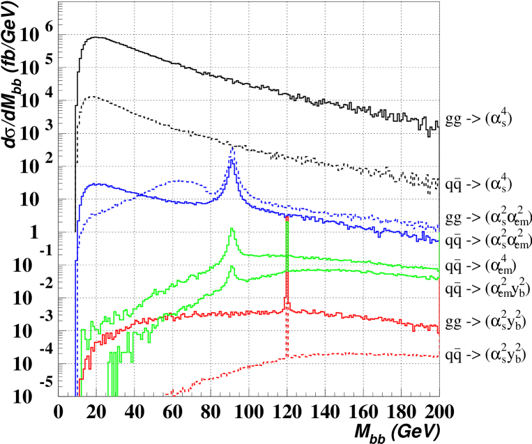
Figure 2: Invariant mass distribution of leading two $b$ quarks in the four-$b$ events generated by GR@PPA_4b. The distribution is shown separately for each subprocess.

ISUB	Initial	Coupling	Total number
	state	order	of diagrams
400	$gg$	$\alpha_{s}^{2}y_{b}^{2}$	48
401	$q\bar{q}$	$\alpha_{s}^{2}y_{b}^{2}$	32
402	$gg$	$\alpha_{s}^{2}\alpha_{em}^{2}$	96
403	$q\bar{q}$	$\alpha_{s}^{2}\alpha_{em}^{2}$	192
404	$q\bar{q}$	$\alpha_{em}^{2}y_{b}^{2}$	80
405	$gg$	$\alpha_{s}^{4}$	76
406	$q\bar{q}$	$\alpha_{s}^{4}$	56
407	$q\bar{q}$	$\alpha_{em}^{4}$	192

Table 1: Eight subprocesses implemented in GR@PPA_4b are listed in the order of the assigned ISUB number. The subprocesses are classified according to the difference in the initial-state parton combination and the coupling order. The total number of diagrams included are also listed for each subprocess in unitary gauge.

Variable	Description
ibswrt	0: BASES is called in the initialization.
	1: A previous BASES result is reused.
icoup	Choice of the energy scale ($Q^{2}$) for couplings
	1: $\hat{s}$ of the hard interaction
	2: Average of the squared transverse mass of $b$ quarks ($<m_{T}^{2}>$)
	3: Sum of the squared transverse mass of $b$ quarks ($\sum m_{T}^{2}$)
	4: Maximum of the squared transverse mass of $b$ quarks ($max$ $m_{T}^{2}$)
	5: Constant value (Set grcq in GeV.)
	6: User defineded energy scale defined in the subroutine grcusrsetq.
ifact	Choice of the energy scale ($Q^{2}$) for PDF
	The definitions are the same as icoup.
	If ifact = 5: Constant value (Set grcfaq in GeV.)
	If not set explicitly, this is taken as the same as icoup.
ncall	Number of sampling points per iteration in BASES
grcfile	Output file name of the BASES result
	A new file if ibswrt = 0; an existing file if ibswrt = 1.

Table 2: Initialization parameters to be specified in the subroutine grcpar.

ISUB	$Q^{2}$	$\sigma$(pb)	$\sigma$(pb)
		Tevatron II	LHC
400	$M_{H}^{2}$	3.409(8) $\times$ 10-3	5.37(1) $\times$ 10-1
401	$M_{H}^{2}$	4.296(8) $\times$ 10-5	4.093(5) $\times$ 10-4
402	$M_{Z}^{2}$	1.924(5)	1.595(4) $\times$ 102
403	$M_{Z}^{2}$	3.129(8)	2.598(4) $\times$ 101
404	$M_{H}^{2}$+M${}_{Z}^{2}$	1.095(2) $\times$ 10-2	9.391(8) $\times$ 10-2
405	$<m_{T}^{2}>$	2.588(5) $\times$ 104	7.56(1) $\times$ 105
406	$<m_{T}^{2}>$	3.413(8) $\times$ 102	1.676(1) $\times$ 103
407	2$M_{Z}^{2}$	2.698(5) $\times$ 10-2	2.568(2) $\times$ 10-1

Table 3: The total cross section estimated by GR@PPA_4b. Results are presented for the cases of Tevatron Run-II and LHC, with CTEQ5L in PYTHIA 6.1 for PDF and without applying any phase-space cut. The Higgs-boson mass is assumed to be 120 GeV/$c^{2}$.

ISUB	ncall	Integration	Integration	Generation	Generation
		accuracy (%)	time (hour)	efficiency (%)	speed (evts/sec)
400	300000	0.258	2.31	2.18	7.5
401	10000	0.204	0.01	53.39	834
402	1000000	0.274	27.38	0.52	0.78
403	200000	0.280	4.00	3.30	4.4
404	20000	0.203	0.03	37.94	386
405	100000	0.207	2.58	6.76	6.6
406	10000	0.238	1.57	48.05	265
407	100000	0.206	0.97	10.67	27

Table 4: The performance of GR@PPA_4b is summarized for each subprocess. Tests were done using a Linux PC (ALPHA 700 MHz) in the Tevatron Run-II condition, with CTEQ5L in PYTHIA 6.1 for PDF and without applying any phase-space cut. The integration accuracy and the integration time are relevant to the execution of BASES at the initialization stage. The generation efficiency and the generation speed show the performance of the SPRING execution. The generation speed does not include the time consumed for the parton showers, hadronization and decays by PYTHIA.

Appendix A Feynman diagrams

Typical Feynman diagrams of the interactions implemented in GR@PPA_4b are illustrated in Figs. 3-7.

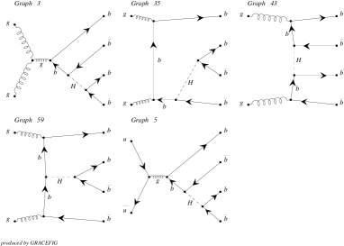
Figure 3: Typical Feynman diagrams having a coupling order of $\alpha_{s}^{2}y_{b}^{2}$.

Figure 4: Typical Feynman diagrams having a coupling order of $\alpha_{s}^{2}\alpha_{em}^{2}$.

Figure 5: Typical Feynman diagrams having a coupling order of $\alpha_{em}^{2}y_{b}^{2}$.

Figure 6: Typical Feynman diagrams having a coupling order of $\alpha_{s}^{4}$.

Figure 7: Typical Feynman diagrams having a coupling order of $\alpha_{em}^{4}$.

Appendix B Sample code

C Program : sample_pyth.F
C Purpose : Sample code to connect to PYTHIA 6.1xx
C Date    : Dec.10.2001
C Author  : Soushi Tsuno

C Only those subprocesses in which a Higgs boson decaying to a
C b-quark pair is produced in association with a b-quark pair
C production via QCD (ISUB = 400 and 401) are activated in this
C example.

C...All real arithmetic in double precision.
      implicit double precision(a-h,o-z)
C...Three Pythia functions return integers, so need declaring.
      integer pyk,pychge,pycomp
C...EXTERNAL statement links PYDATA on most machines.
      external pydata
C...Commonblocks.
      common/pyjets/n,npad,k(4000,5),p(4000,5),v(4000,5)
      common/pypars/mstp(200),parp(200),msti(200),pari(200)
      common/pydat1/mstu(200),paru(200),mstj(200),parj(200)
      common/pysubs/msel,mselpd,msub(500),kfin(2,-40:40),ckin(200)

C...Counter for number of generated events of each type.
      dimension ncount(8)
      data ncount/8*0/

C...Include GR@PPA common parameter.
      include ’./inc/grchad.inc’

C...Set Ntuple-----------------------------------------------------
      integer nwpawc
      parameter (nwpawc=300000)
      common/pawc/paw(nwpawc)
      integer neve,psub
      real pj
      common/genep/neve,psub,pj(5,6)

      call hlimit(nwpawc)
      call hropen(1,’genep’,’bbbb_tev.nt’,’N’,4095,istat)
      call hbnt(10,’genep’,’ ’)
      call hbname(10,’genep’,neve,’neve:i,psub:i,pj(5,6):r’)
C-----------------------------------------------------------------

C...Number of events and cm energy.
      nev = 1000                ! Number of events
      grcecm = 2000.0d0         ! CM Energy

C...Kinematical cuts.
      gptcut   = 0.0d0          ! Pt Cut for each particles
      getacut  = 100.0d0        ! Eta Cut
      grconcut = 0.0d0          ! RCone Cut
C   Other cuts can be applies using CKIN parameters of Pythia.
C   Furthermore, users can define their own cuts by editing the
C   subroutine grcusrcut in grcpar.F.

C...PDF and Coupling.
C   These parameters have to be set before the GR@PPA_4b initialization.
      mstp(51)  = 7             ! CTEC5L
      mstp(58)  = 4             ! Nr. of flavor in PDF
      mstu(101) = 1             ! running alpha_em
      iord_als  = 1             ! first-order running alpha_s
      nfrv_als  = 5             ! Nr. of flavors assumed in alpha_s
      aLam_als  = 0.146d0       ! Lambda used in alpha_s

      mstu(111) = iord_als
      mstu(112) = nfrv_als
      paru(112) = aLam_als

C...GR@PPA_4b initialization (BASES integration).
      call grcpygen(’PAP’,400,1,sigmax) ! gg -> h0(bb)+bb(Higgs2,QCD2)
      call grcpygen(’PAP’,401,1,sigmax) ! qq -> h0(bb)+bb(Higgs2,QCD2)

C...Pythia initialization.
      msel = 0
      msub(400) = 1         ! External process on
      msub(401) = 1         ! External process on
C   Switch off unnecessary aspects of Pythia.
C      mstp(61)  = 0             ! Initial state radiation OFF
C      mstp(71)  = 0             ! Final state radiation OFF
C      mstp(81)  = 0             ! Multiple interaction OFF
C      mstp(111) = 0             ! Hadronization OFF
C   Initialization.
      call pyinit(’CMS’,’p’,’pbar’,grcecm)

C...The alpha_s parameters must be set again here if they are non-
C   standard. These parameters are over-written with standard ones
C   in pyinit according the choice of PDF.
      mstu(111) = iord_als
      mstu(112) = nfrv_als
      paru(112) = aLam_als

C...Event loop.
      do iev = 1,nev

         call pyevnt

         isub = msti(1)
         icase = 1
         if (isub.ge.400 .and. isub.le.407) icase = isub - 399
         ncount(icase) = ncount(icase) + 1
         if (ncount(icase).le.1) then
            write(6,*) ’ Following event is subprocess’,isub
            call pylist(1)
         endif

         if (mod(iev,1000).eq.0) then
            write(*,*) iev
         endif

C...Data Store.

C...Event Nr..
         neve = iev
C...Process ID.
         psub = isub

C...Set Particle 1,2 (x,y,z).
         do i = 1,2
            do j = 1,4
               pj(j,i) = p(i+2,j)
            enddo
            pj(5,i) = k(i+2,2)
         enddo

C...Set Particle 3,4,5,6 (pt,phi,eta).
         do i = 3,6
            pj(1,i) = pyp(i+4,10)
            pj(2,i) = pyp(i+4,15)
            pj(3,i) = pyp(i+4,19)
            pj(4,i) = pyp(i+4,4)
            pj(5,i) = k(i+4,2)
         enddo

C...Fill ntuple.
         call hfnt(10)

C...End of loop over events.
      enddo

C...Cross section table.
      call pystat(1)

C...Close ntuple.
      call hrout(10,genep,’ ’)
      call hrend(’genep’)

      end


C###########################################################
      subroutine pyupev(isub,sigev)
      implicit double precision(a-h,o-z)
      integer isub
      real*8 sigev

C...Only call GR@PPA_4b.
      call grcpygen(’ ’,isub,0,sigev)

      return
      end

Appendix C Test run output

 ******************************************************************************
 ******************************************************************************
 **  Welcome to                                                              **
 **                                                                          **
 **       GGG  RRRR          PPPP  PPPP   AAA                                **
 **      G   G R   R   @@@@  P   P P   P A   A                               **
 **      G     R   R  @ @@ @ P   P P   P A   A                               **
 **      G GGG RRRR  @ @ @ @ PPPP  PPPP  AAAAA                               **
 **      G   G R  R  @ @@ @  P     P     A   A                               **
 **       GGG  R   R  @@@@@@ P     P     A   A  _4b                          **
 **     =======================================                              **
 **       GRace At Proton-Proton/Anti-proton                                 **
 **                                                                          **
 **       This is GR@PPA version 1.0                                         **
 **       coded by S.Tsuno (tsuno@fnal.gov)                                  **
 **       with Minami Tateya Collab. and ATLAS-J.                            **
 **                                                                          **
 **       On web...  http://www.kek.jp/                                      **
 **       Referances, ........                                               **
 **                                                                          **
 ******************************************************************************
 ******************************************************************************
 Accepted CM Energy :   2000.00000000000      GeV
          Beam type : Proton-Anti-Proton Collision
 Process : [         400 ] gg -> h0(bb)+bb(Higgs2,QCD2)
 Set BASES file
    Filename : bases_400_mh120.result
               bases_400_mh120.data
           4  body final state
   Pt Cut of Particle           1  : none
   Pt Cut of Particle           2  : none
   Pt Cut of Particle           3  : none
   Pt Cut of Particle           4  : none
   Eta Cut of Particle           1  : none
   Eta Cut of Particle           2  : none
   Eta Cut of Particle           3  : none
   Eta Cut of Particle           4  : none
   Rcone Cut of Particle           1  : none
   Rcone Cut of Particle           2  : none
   Rcone Cut of Particle           3  : none
   Rcone Cut of Particle           4  : none
   Missing Pt(Et) Cut : none
   Option of Renormalization Scale :           5   120.000000000000      GeV
   Option of   Factorization Scale :           0

 Start BASES Integration!!


                                                       Date:  2/ 2/20  05:03
        **********************************************************
        *                                                        *
        *     BBBBBBB     AAAA     SSSSSS   EEEEEE   SSSSSS      *
        *     BB    BB   AA  AA   SS    SS  EE      SS    SS     *
        *     BB    BB  AA    AA  SS        EE      SS           *
        *     BBBBBBB   AAAAAAAA   SSSSSS   EEEEEE   SSSSSS      *
        *     BB    BB  AA    AA        SS  EE            SS     *
        *     BB    BB  AA    AA  SS    SS  EE      SS    SS     *
        *     BBBB BB   AA    AA   SSSSSS   EEEEEE   SSSSSS      *
        *                                                        *
        *                   BASES Version 5.1                    *
        *           coded by S.Kawabata KEK, March 1994          *
        **********************************************************

     <<   Parameters for BASES    >>

      (1) Dimensions of integration etc.
          # of dimensions :    Ndim    =       10   ( 50 at max.)
          # of Wilds      :    Nwild   =       10   ( 15 at max.)
          # of sample points : Ncall   =   299008(real)   300000(given)
          # of subregions    : Ng      =       50 / variable
          # of regions       : Nregion =        2 / variable
          # of Hypercubes    : Ncube   =     1024

      (2) About the integration variables
          ------+---------------+---------------+-------+-------
              i       XL(i)           XU(i)       IG(i)   Wild
          ------+---------------+---------------+-------+-------
              1    0.000000E+00    1.000000E+00     1      yes
              2    0.000000E+00    1.000000E+00     1      yes
              3    0.000000E+00    1.000000E+00     1      yes
              4    0.000000E+00    1.000000E+00     1      yes
              5    0.000000E+00    1.000000E+00     1      yes
              6    0.000000E+00    1.000000E+00     1      yes
              7    0.000000E+00    1.000000E+00     1      yes
              8    0.000000E+00    1.000000E+00     1      yes
              9    0.000000E+00    1.000000E+00     1      yes
             10    0.000000E+00    1.000000E+00     1      yes
          ------+---------------+---------------+-------+-------

      (3) Parameters for the grid optimization step
          Max.# of iterations: ITMX1 =        5
          Expected accuracy  : Acc1  =   0.2000 %

      (4) Parameters for the integration step
          Max.# of iterations: ITMX2 =        5
          Expected accuracy  : Acc2  =   0.0100 %


                                                       Date:  2/ 2/20  05:03
               Convergency Behavior for the Grid Optimization Step
 ------------------------------------------------------------------------------
 <- Result of  each iteration ->  <-     Cumulative Result     -> < CPU  time >
  IT Eff R_Neg   Estimate  Acc %  Estimate(+- Error )order  Acc % ( H: M: Sec )
 ------------------------------------------------------------------------------
   1  99  0.00  3.417E-03  0.902  3.417196(+-0.030830)E-03  0.902   0:14: 2.08
   2  99  0.00  3.460E-03  0.669  3.444653(+-0.018513)E-03  0.537   0:28: 4.14
   3  99  0.00  3.421E-03  0.583  3.433936(+-0.013571)E-03  0.395   0:42: 6.15
   4  99  0.00  3.404E-03  0.573  3.424234(+-0.011139)E-03  0.325   0:56: 8.20
   5  99  0.00  3.438E-03  0.572  3.427558(+-0.009692)E-03  0.283   1:10:10.26
 ------------------------------------------------------------------------------


                                                       Date:  2/ 2/20  05:03
               Convergency Behavior for the Integration Step
 ------------------------------------------------------------------------------
 <- Result of  each iteration ->  <-     Cumulative Result     -> < CPU  time >
  IT Eff R_Neg   Estimate  Acc %  Estimate(+- Error )order  Acc % ( H: M: Sec )
 ------------------------------------------------------------------------------
   1  99  0.00  3.407E-03  0.579  3.406833(+-0.019711)E-03  0.579   1:24:12.01
   2  99  0.00  3.378E-03  0.580  3.392381(+-0.013901)E-03  0.410   1:38:13.74
   3  99  0.00  3.424E-03  0.578  3.402792(+-0.011373)E-03  0.334   1:52:15.38
   4  99  0.00  3.423E-03  0.574  3.407759(+-0.009841)E-03  0.289   2: 6:16.63
   5  99  0.00  3.416E-03  0.570  3.409380(+-0.008783)E-03  0.258   2:20:18.34
 ------------------------------------------------------------------------------


                    ****** END OF BASES *********

     <<   Computing Time Information   >>

               (1) For BASES              H: M:  Sec
                   Overhead           :   0: 0: 0.00
                   Grid Optim. Step   :   1:10:10.26
                   Integration Step   :   1:10: 8.08
                   Go time for all    :   2:20:18.34

               (2) Expected event generation time
                   Expected time for 1000 events :      4.02 Sec
 ******************************************************************************
 ******************************************************************************
 **  Welcome to                                                              **
 **                                                                          **
 **       GGG  RRRR          PPPP  PPPP   AAA                                **
 **      G   G R   R   @@@@  P   P P   P A   A                               **
 **      G     R   R  @ @@ @ P   P P   P A   A                               **
 **      G GGG RRRR  @ @ @ @ PPPP  PPPP  AAAAA                               **
 **      G   G R  R  @ @@ @  P     P     A   A                               **
 **       GGG  R   R  @@@@@@ P     P     A   A  _4b                          **
 **     =======================================                              **
 **       GRace At Proton-Proton/Anti-proton                                 **
 **                                                                          **
 **       This is GR@PPA version 1.0                                         **
 **       coded by S.Tsuno (tsuno@fnal.gov)                                  **
 **       with Minami Tateya Collab. and ATLAS-J.                            **
 **                                                                          **
 **       On web...  http://www.kek.jp/                                      **
 **       Referances, ........                                               **
 **                                                                          **
 ******************************************************************************
 ******************************************************************************
 Accepted CM Energy :   2000.00000000000      GeV
          Beam type : Proton-Anti-Proton Collision
 Process : [         401 ] qq -> h0(bb)+bb(Higgs2,QCD2)
 Set BASES file
    Filename : bases_401_mh120.result
               bases_401_mh120.data
           4  body final state
   Pt Cut of Particle           1  : none
   Pt Cut of Particle           2  : none
   Pt Cut of Particle           3  : none
   Pt Cut of Particle           4  : none
   Eta Cut of Particle           1  : none
   Eta Cut of Particle           2  : none
   Eta Cut of Particle           3  : none
   Eta Cut of Particle           4  : none
   Rcone Cut of Particle           1  : none
   Rcone Cut of Particle           2  : none
   Rcone Cut of Particle           3  : none
   Rcone Cut of Particle           4  : none
   Missing Pt(Et) Cut : none
   Option of Renormalization Scale :           5   120.000000000000      GeV
   Option of   Factorization Scale :           0

 Start BASES Integration!!


                                                       Date:  2/ 2/20  07:24
        **********************************************************
        *                                                        *
        *     BBBBBBB     AAAA     SSSSSS   EEEEEE   SSSSSS      *
        *     BB    BB   AA  AA   SS    SS  EE      SS    SS     *
        *     BB    BB  AA    AA  SS        EE      SS           *
        *     BBBBBBB   AAAAAAAA   SSSSSS   EEEEEE   SSSSSS      *
        *     BB    BB  AA    AA        SS  EE            SS     *
        *     BB    BB  AA    AA  SS    SS  EE      SS    SS     *
        *     BBBB BB   AA    AA   SSSSSS   EEEEEE   SSSSSS      *
        *                                                        *
        *                   BASES Version 5.1                    *
        *           coded by S.Kawabata KEK, March 1994          *
        **********************************************************

     <<   Parameters for BASES    >>

      (1) Dimensions of integration etc.
          # of dimensions :    Ndim    =       11   ( 50 at max.)
          # of Wilds      :    Nwild   =       11   ( 15 at max.)
          # of sample points : Ncall   =     8192(real)    10000(given)
          # of subregions    : Ng      =       50 / variable
          # of regions       : Nregion =        2 / variable
          # of Hypercubes    : Ncube   =     2048

      (2) About the integration variables
          ------+---------------+---------------+-------+-------
              i       XL(i)           XU(i)       IG(i)   Wild
          ------+---------------+---------------+-------+-------
              1    0.000000E+00    1.000000E+00     1      yes
              2    0.000000E+00    1.000000E+00     1      yes
              3    0.000000E+00    1.000000E+00     1      yes
              4    0.000000E+00    1.000000E+00     1      yes
              5    0.000000E+00    1.000000E+00     1      yes
              6    0.000000E+00    1.000000E+00     1      yes
              7    0.000000E+00    1.000000E+00     1      yes
              8    0.000000E+00    1.000000E+00     1      yes
              9    0.000000E+00    1.000000E+00     1      yes
             10    0.000000E+00    1.000000E+00     1      yes
             11    0.000000E+00    1.000000E+00     1      yes
          ------+---------------+---------------+-------+-------

      (3) Parameters for the grid optimization step
          Max.# of iterations: ITMX1 =        5
          Expected accuracy  : Acc1  =   0.2000 %

      (4) Parameters for the integration step
          Max.# of iterations: ITMX2 =        5
          Expected accuracy  : Acc2  =   0.0100 %


                                                       Date:  2/ 2/20  07:24
               Convergency Behavior for the Grid Optimization Step
 ------------------------------------------------------------------------------
 <- Result of  each iteration ->  <-     Cumulative Result     -> < CPU  time >
 ------------------------------------------------------------------------------
   1  99  0.00  4.288E-05  1.449  4.287773(+-0.062123)E-05  1.449   0: 0: 2.62
   2  99  0.00  4.291E-05  0.620  4.290673(+-0.024461)E-05  0.570   0: 0: 5.25
   3  99  0.00  4.311E-05  0.457  4.303146(+-0.015345)E-05  0.357   0: 0: 7.88
   4  99  0.00  4.311E-05  0.455  4.306190(+-0.012091)E-05  0.281   0: 0:10.50
   5  99  0.00  4.290E-05  0.430  4.301289(+-0.010110)E-05  0.235   0: 0:13.12
 ------------------------------------------------------------------------------


                                                       Date:  2/ 2/20  07:24
               Convergency Behavior for the Integration Step
 ------------------------------------------------------------------------------
 <- Result of  each iteration ->  <-     Cumulative Result     -> < CPU  time >
  IT Eff R_Neg   Estimate  Acc %  Estimate(+- Error )order  Acc % ( H: M: Sec )
 ------------------------------------------------------------------------------
   1  99  0.00  4.296E-05  0.446  4.295959(+-0.019145)E-05  0.446   0: 0:15.74
   2  99  0.00  4.295E-05  0.458  4.295262(+-0.013719)E-05  0.319   0: 0:18.36
   3  99  0.00  4.316E-05  0.482  4.301655(+-0.011453)E-05  0.266   0: 0:20.98
   4  99  0.00  4.291E-05  0.452  4.298948(+-0.009860)E-05  0.229   0: 0:23.60
   5  99  0.00  4.290E-05  0.430  4.297026(+-0.008694)E-05  0.202   0: 0:26.22
 ------------------------------------------------------------------------------


                    ****** END OF BASES *********

     <<   Computing Time Information   >>

               (1) For BASES              H: M:  Sec
                   Overhead           :   0: 0: 0.00
                   Grid Optim. Step   :   0: 0:13.12
                   Integration Step   :   0: 0:13.09
                   Go time for all    :   0: 0:26.22

               (2) Expected event generation time
                   Expected time for 1000 events :      0.46 Sec
1
 ******************************************************************************
 ******************************************************************************
 **                                                                          **
 **                                                                          **
 **              *......*                  Welcome to the Lund Monte Carlo!  **
 **         *:::!!:::::::::::*                                               **
 **      *::::::!!::::::::::::::*          PPP  Y   Y TTTTT H   H III   A    **
 **    *::::::::!!::::::::::::::::*        P  P  Y Y    T   H   H  I   A A   **
 **   *:::::::::!!:::::::::::::::::*       PPP    Y     T   HHHHH  I  AAAAA  **
 **   *:::::::::!!:::::::::::::::::*       P      Y     T   H   H  I  A   A  **
 **    *::::::::!!::::::::::::::::*!       P      Y     T   H   H III A   A  **
 **      *::::::!!::::::::::::::* !!                                         **
 **      !! *:::!!:::::::::::*    !!       This is PYTHIA version 6.138      **
 **      !!     !* -><- *         !!       Last date of change:  2 Mar 2000  **
 **      !!     !!                !!                                         **
 **      !!     !!                !!       Now is 20 Feb 2002 at  7:24:31    **
 **      !!                       !!                                         **
 **      !!        ep             !!       Disclaimer: this program comes    **
 **      !!                       !!       without any guarantees. Beware    **
 **      !!                 pp    !!       of errors and use common sense    **
 **      !!   e+e-                !!       when interpreting results.        **
 **      !!                       !!                                         **
 **      !!                                Copyright T. Sjostrand (1999)     **
 **                                                                          **
 ** An archive of program versions and documentation is found on the web:    **
 ** http://www.thep.lu.se/~torbjorn/Pythia.html                              **
 **                                                                          **
 ** When you cite this program, currently the official reference is          **
 ** T. Sjostrand, Computer Physics Commun. 82 (1994) 74.                     **
 ** The supersymmetry extensions are described in                            **
 ** S. Mrenna, Computer Physics Commun. 101 (1997) 232                       **
 ** Also remember that the program, to a large extent, represents original   **
 ** physics research. Other publications of special relevance to your        **
 ** studies may therefore deserve separate mention.                          **
 **                                                                          **
 ** Main author: Torbjorn Sjostrand; Department of Theoretical Physics 2,    **
 **   Lund University, Solvegatan 14A, S-223 62 Lund, Sweden;                **
 **   phone: + 46 - 46 - 222 48 16; e-mail: torbjorn@thep.lu.se              **
 ** SUSY author: Stephen Mrenna, Physics Department, UC Davis,               **
 **   One Shields Avenue, Davis, CA 95616, USA;                              **
 **   phone: + 1 - 530 - 752 - 2661; e-mail: mrenna@physics.ucdavis.edu      **
 **                                                                          **
 **                                                                          **
 ******************************************************************************
 ******************************************************************************
1****************** PYINIT: initialization of PYTHIA routines *****************

 ==============================================================================
 I                                                                            I
 I             PYTHIA will be initialized for a p on pbar collider            I
 I                  at   2000.000 GeV center-of-mass energy                   I
 I                                                                            I
 ==============================================================================

 ******** PYMAXI: summary of differential cross-section maximum search ********

           ==========================================================
           I                                      I                 I
           I  ISUB  Subprocess name               I  Maximum value  I
           I                                      I                 I
           ==========================================================
           I                                      I                 I
           I   96   Semihard QCD 2 -> 2           I    6.6438D+02   I
           I  400   gg -> h0(bb)+bb(Higgs2,QCD2)  I    3.4094D-12   I
           I  401   qq -> h0(bb)+bb(Higgs2,QCD2)  I    4.2971D-14   I
           I                                      I                 I
           ==========================================================

 ********************** PYINIT: initialization completed **********************
  Following event is subprocess         400


  !!! Event lists by PYTHIA are omitted....


1********* PYSTAT:  Statistics on Number of Events and Cross-sections *********

 ==============================================================================
 I                                  I                            I            I
 I            Subprocess            I      Number of points      I    Sigma   I
 I                                  I                            I            I
 I----------------------------------I----------------------------I    (mb)    I
 I                                  I                            I            I
 I N:o Type                         I    Generated         Tried I            I
 I                                  I                            I            I
 ==============================================================================
 I                                  I                            I            I
 I   0 All included subprocesses    I         1000          1000 I  3.452D-12 I
 I 400 gg -> h0(bb)+bb(Higgs2,QCD2) I          990           990 I  3.409D-12 I
 I 401 qq -> h0(bb)+bb(Higgs2,QCD2) I           10            10 I  4.297D-14 I
 I                                  I                            I            I
 ==============================================================================

 ********* Fraction of events that fail fragmentation cuts =  0.00000 *********

References

- [1] M. Carena et al., Report of the Tevatron Higgs Working Group, hep-ph/0010338 (2000).
-
[2]
ATLAS Technical Proporsal, CERN/LHCC/94-43 (1994);
CMS Technical Proporsal, CERN/LHCC/94-38 (1994). -
[3]
For reviews, H.P. Nilles, Phys. Rep. 110, 1 (1984);
H.E. Haber and G.L. Kane, Phys. Rep. 117, 75 (1985). -
[4]
J. Dai, J.F. Gunion, and R. Vega,
Phys. Lett. B 345, 29 (1995);
J. Dai, J.F. Gunion, and R. Vega, Phys. Lett. B 387, 801 (1996). - [5] CDF Collab., T. Affolder et al., Phys. Rev. Lett. 86, 4472 (2001).
- [6] E. Richter-Wa̧s, and D. Froidevaux, Z. Phys. C 76, 665 (1997).
-
[7]
T. Ishikawa et al., GRACE manual,
KEK Report 92-19 (1993);
F. Yuasa et al., Prog. Theor. Phys. Suppl. 138, 18 (2000); hep-ph/0007053. - [8] K. Sato et al., Proc. VII International Workshop on Advanced Computing and Analysis Techniques in Physics Research (ACAT 2000), P.C. Bhat and M. Kasemann, AIP Conference Proceedings 583 214 (2001).
-
[9]
S. Kawabata, Comput. Phys. Commun. 41, 466 (1985);
S. Kawabata, Comput. Phys. Commun. 88, 309 (1995). - [10] T. Sjöstrand, Comput. Phys. Commun. 82, 74 (1994).
- [11] T. Abe, Comput. Phys. Commun. 136, 126 (2001).
- [12] J. Fujimoto et al., Comput. Phys. Commun. 100, 128 (1997).
- [13] PAW: Physics Analysis Workstation, CERN Program Library Long Writeup Q121.
- [14] H. Plothow-Besch, Comput. Phys. Commun. 75, 396 (1993).
- [15] CTEQ Collab.,H.L. Lai et al., Eur. Phys. J. C 12, 375 (2000).
-
[16]
A. Pukhov et al.,
CompHEP - a package for evaluation of Feynman diagrams and integration
over multi-particle phase space. User’s manual for version 33.,
hep-ph/9908288 (1999);
V. Ilyin, private communication.