Two Photon Width of $\eta_{c}$

Abstract

We discuss the measured partial width of the pseudoscalar charmonium state $\eta_{c}$ into two photons. Predictions from potential models are examined and compared with experimental values. Including radiative corrections, it is found that present measurements are compatible both with a QCD type potential and with a static Coulomb potential. The latter is then used to give an estimate on the $\eta_{b}$ decay into two photons. Results for $\eta_{c}$ are also compared with those from $J/\psi$ data through the NRQCD model.

1 Introduction

In this paper we revisit the calculation of the two photon width of $\eta_{c}$, highlighting newest experimental results and updating the potential model calculation. This allows for a reliable estimate of the two photon width of $\eta_{b}$, which is been searched for in $\gamma\gamma$ collisions [1]. We shall see that the expected two photon width of $\eta_{b}$ is within reach of the precision in the LEP data being analyzed.

The charmonium spectrum has been the basic testing grounds for a variety of models for the interquark potential, ever since the discovery of the $J/\psi$ in 1974 [2]. The experimental scenario describing the $c{\bar{c}}$ bound states is close to completion, with the observed higher excitation states ${}^{3}P_{0}$, ${}^{3}P_{1}$ and spin 2 ${}^{3}P_{2}$ states [3] : decay widths into various leptonic and hadronic states have been measured and compared with potential models [4, 5]. Most of this note is dedicated to examine the theoretical predictions for the electromagnetic decay of the simplest and lowest lying of all the charmonium states, i.e. the pseudoscalar $\eta_{c}$. In Sect. 2 we shall compare the two photon decay width with the leptonic width of the $J/\psi$, which has been measured with higher precision [6] and found to be 15% higher than in previous measurements [7]. This implies that a number of potential models whose parameters had been determined by the leptonic width of the $J/\psi$ may need some updating, and so do some predictions from these models. Potential model predictions for $\eta_{c}\to\gamma\gamma$ can be found in Sect. 3, together with a value for the two photon width of $\eta_{b}$ extracted from the Coulombic potential. In Sect. 4 we show the predictions for $\eta_{c}$ decay widths, using the procedure introduced in [8] for the description of mesons made out of two non relativistic heavy quarks, by means of the Non Relativistic Quantum Chromodynamics–NRQCD. In Sect. 5 we compare these different determinations with the experimental value of the $\eta_{c}\to\gamma\gamma$ decay width expanding some recent theoretical analyses on this subject (see for instance [9], [10] and references therein).

2 Experimental values and relation to $J/\psi$ electromagnetic width

The first evidence of the $\eta_{c}$ state has been found in the inclusive photon spectra of the $\psi^{\prime}$ and $J/\psi$ decays [11], [12]. Subsequently, through $\gamma\gamma$ collisions, the decay width of $\eta_{c}$ into two photons has been measured in different experiments. The most recently reported values for the radiative decay width are shown in fig. (1) [13, 14, 15, 16, 17, 18, 19, 20, 21, 22],

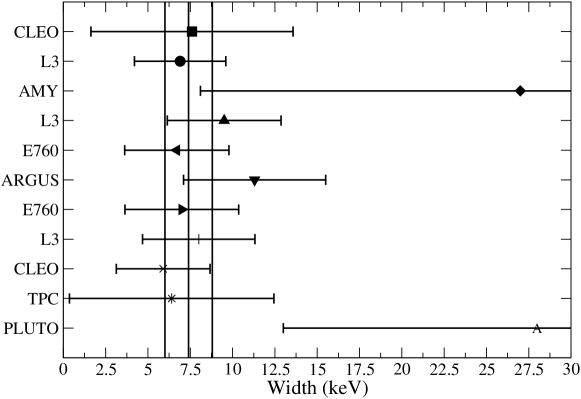
Figure 1: Experimental values of various measures of $\eta_{c}\to\gamma\gamma$

together with the Particle Data Group average [23], which reads

$$\Gamma_{exp}(\eta_{c}\to\gamma\gamma)=7.4\pm 1.4\textrm{ keV .}$$ (1)

In order to compare the experimental determinations with theoretical expectations, we start with the two photon decay width of a pseudoscalar quark-antiquark bound state [24] with first order QCD corrections [25], which can be written as

$$\Gamma(\eta_{c}\rightarrow\gamma\gamma)=\Gamma_{B}^{P}\left[1+\frac{\alpha_{s}}{\pi}\left(\frac{\pi^{2}-20}{3}\right)\right].$$ (2)

In eq. (2), $\Gamma_{B}^{P}$ is the Born decay width for a non-relativistic bound state which can be calculated from potential models. A first theoretical estimate for this decay width can be obtained by comparing eq. (2) with the expressions for the vector state $J/\psi$ [26], i.e.

$$\Gamma(J/\psi\rightarrow e^{+}e^{-})=\Gamma_{B}^{V}\left(1-\frac{16}{3}\frac{\alpha_{s}}{\pi}\right).$$ (3)

The expressions in eqs. (2) and (3) can be used to estimate the radiative width of $\eta_{c}$ from the measured values of the leptonic decay width of $J/\psi$, if one assumes the same value for the wave function at the origin $\psi(0)$, for both the pseudoscalar and the vector state. This is true up to errors of $\mathcal{O}(\alpha_{s}/m_{c}^{2})$ (see for instance [27, 28]).

Taking the ratio between eqs. (2) and (3) and expanding in $\alpha_{s}$, we obtain

$$\frac{\Gamma(\eta_{c}\rightarrow\gamma\gamma)}{\Gamma(J/\psi\rightarrow e^{+}e^{-})}\approx\frac{4}{3}\frac{(1-3.38\alpha_{s}/\pi)}{(1-5.34\alpha_{s}/\pi)}=\frac{4}{3}\left[1+1.96\frac{\alpha_{s}}{\pi}+\mathcal{O}(\alpha_{s}^{2})\right]$$ (4)

The correction can be computed from the two loop expression for $\alpha_{s}$ and the value [23] $\alpha_{s}(M_{Z})=0.118\pm 0.003$. Using the renormalization group equation to evaluate $\alpha_{s}(Q=2m_{c}=3.0\mbox{ GeV})=0.25\pm 0.01$, and the latest measurement

$$\Gamma_{exp}(J/\psi\rightarrow e^{+}e^{-})=5.26\pm 0.37\textrm{ keV}$$ (5)

one obtains

$$\Gamma(\eta_{c}\rightarrow\gamma\gamma)\pm\Delta\Gamma(\eta_{c}\rightarrow\gamma\gamma)=8.18\pm 0.57\pm 0.04\ \ \textrm{keV}$$ (6)

where the first error comes from the uncertainty on the $J/\psi$ experimental width, the second error from $\alpha_{s}$ . This estimate agrees within $1\sigma$ with the value given in eq. (1). Here we assumed the $\alpha_{s}$ scale to be $Q=2m_{c}=3.0\textrm{ GeV}$. This choice is by no way unique, and in fig. (2) we show the dependence of the $\eta_{c}$ photonic width, evaluated from eq. (5), upon different values of the scale chosen for $\alpha_{s}$.

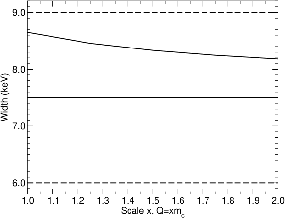
Figure 2: The dependence of the $\eta_{c}$ decay width to $\gamma\gamma$ (in keV) is shown with respect to the scale chosen for $\alpha_{s}$  in the radiative corrections. The horizontal lines represent the central experimental value (full line) and the (dashed lines) indetermination.

As one can see from fig. (2) the experimental width value is not sufficient to uniquely determine the a scale choice of $\alpha_{s}$ . We shall therefore include this fluctuation in the indetermination due to radiative corrections.

3 Potential models predictions for $\eta_{c}$ and $\eta_{b}$

We present now the results one can obtain for the absolute width, through the extraction of the wave function at the origin from potential models. For the calculation of the wavefunction we have used four different models, namely the Cornell type potential [27] $V(r)=-\frac{k}{r}+\frac{r}{a^{2}}$ with parameters $a=2.34$ and $k=0.52$, the Richardson potential [30] $V_{R}(r)=-\frac{4}{3}\frac{12\pi}{33-2N_{f}}\int\frac{d^{3}q}{(2\pi)^{3}}\frac{e^{iqr}}{q^{2}\log(1+q^{2}/\Lambda^{2})}$ with $N_{f}=3$ and $\Lambda=398$ $MeV$, and the QCD inspired potential $V_{J}$ of Igi-Ono [31, 32]

$$V_{J}(r)=V_{AR}(r)+dre^{-gr}+ar,\ \ \ V_{AR}(r)=-\frac{4}{3}\frac{\alpha_{s}^{(2)}(r)}{r}$$ (7)

with two different parameter sets, corresponding to $\Lambda_{\overline{MS}}=0.5\ GeV$ and $\Lambda_{\overline{MS}}=0.3\ GeV$ respectively [31]. We also show the results from a Coulombic type potential with the QCD coupling $\alpha_{s}$ frozen to a value of $r$ which corresponds to the Bohr radius of the quarkonium system, obtained by solving the equation $r_{B}=3/(2m_{c}\alpha_{s}(r_{B}))$  [33]. We stress that the scale of $\alpha_{s}$ occurring in the radiative corrections and the one of the Coulombic potential are different[34].

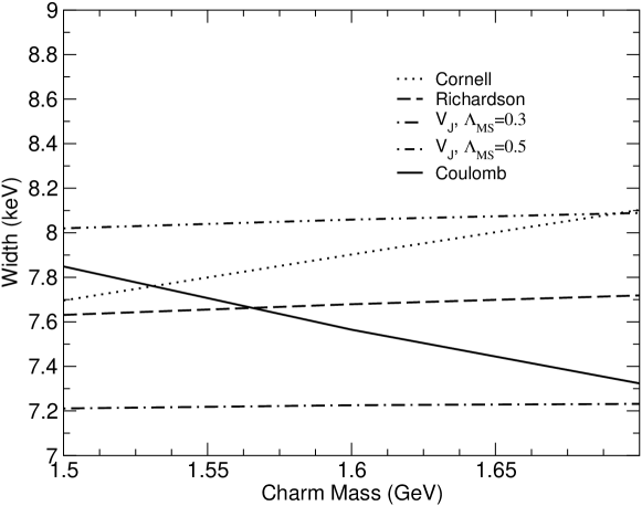
Figure 3: The dependence of $\eta_{c}$ decay width to $\gamma\gamma$ in keV for different potential models is shown as a function of $m_{c}$ .

We show in fig. (3) the predictions for the decay width from these potential models with the correction from eq. (2) at an $\alpha_{s}$ scale $Q=2m_{c}$ , observing that the calculated widths stay well within one standard deviation of the width value given by eq. (1). For any given model, sources of error in this calculation arise from the choice of scale in the radiative correction factor and the choice of the parameters. Including the fluctuations of the results given by the different models, we can estimate a range of values for the potential model predictions for the radiative decay width $\Gamma(\eta_{c}\to\gamma\gamma)$, namely

$$\Gamma(\eta_{c}\to\gamma\gamma)=7.6\pm 1.5\textrm{ keV \mbox{ }.}$$ (8)

ALEPH has recently started to search for $\eta_{b}$ into two photons[35] and it is interesting to see whether the potential models can predict for this decay a value within experimental reach. Predictions of course will be affected by the error due to the parametric dependence of the given potential model, an error which can be quite large since most of the parameters have been tuned with the charmonium system. On the other hand, the Coulombic potential gives results for the charmonium system in agreement with all the other models, and, at the same time, is relatively free of such parameter dependence. With only the scale of $\alpha_{s}$ in the wave function to worry about, it can be used for a reliable estimate. For this purpose we shall make use of the expression in eq. (2) where this time $e_{q}=1/3$ and $m_{b}=5.0\textrm{ GeV}$. This gives the potential model prediction

$$\Gamma(\eta_{b}\rightarrow\gamma\gamma)=0.50\pm 0.03\textrm{ keV}\;,$$ (9)

where the error is associated to different choices of $m_{b}$ values and to the indetermination on $\alpha_{s}$ occurring in the radiative correction. A check of this estimate can be given using the leptonic width of the $\Upsilon$ and the expansion given in eq. (4). To first order in $\alpha_{s}$ one obtains:

$$\frac{\Gamma(\eta_{b}\rightarrow\gamma\gamma)}{\Gamma(\Upsilon\rightarrow e^{+}e^{-})}\approx\frac{1}{3}\frac{(1-3.38\alpha_{s}/\pi)}{(1-5.34\alpha_{s}/\pi)}=\frac{1}{3}\left[1+1.96\frac{\alpha_{s}}{\pi}+\mathcal{O}(\alpha_{s}^{2})\right]$$ (10)

which differs from eq. (4) only by a charge factor; using the PDG average [23]

$$\Gamma_{exp}(\Upsilon\to e^{+}e^{-})=1.32\pm 0.05\textrm{ keV}$$ (11)

and assuming the wavefunctions of the two $b\overline{b}$ bound states to be equal we have

$$\Gamma(\eta_{b}\to\gamma\gamma)=0.49\pm 0.04\textrm{ keV}$$ (12)

in agreement with the Coulombic model prediction eq. (9). For the radiative correction factor we have used $\alpha_{s}(Q=2m_{b}=10\textrm{ GeV})=0.18\pm 0.01$. The associated error in eq. (12) takes into account the indetermination on the experimental value eq. (11) and the one on $\alpha_{s}$ .

A more thorough discussion on the theoretical estimates of the $\eta_{b}$ decay into two photons and comparison to some recent calculations (see for instance [36]) will follow in a future publication [37].

4 Octet component model

We will present now another model which admits other components to the meson decay beyond the one from the colour singlet picture (Bodwin, Braaten and Lepage) [8]. NRQCD has been used to separate the short distance scale of annihilation from the nonperturbative contributions of long distance scale. This model has been successfully used to explain the larger than expected $J/\psi$ production at the Tevatron and LEP. According to BBL, in the octet model for quarkonium, the decay widths of charmonium states are given by:

$$\Gamma(J/\psi\to LH) = \frac{2\langle J/\psi|O_{1}(^{3}S_{1})|J/\psi\rangle}{m_{c}^{2}}\frac{10\alpha_{s}^{2}(\pi^{2}-9)}{243}\times$$

$$\times\left[\alpha_{s}\left(1-3.7\frac{\alpha_{s}}{\pi}\right)\right. + 3.2\alpha\left(1-6.7\frac{\alpha_{s}}{\pi}\left.\right)\right]-$$ (13)

$$- \frac{2\langle J/\psi|P_{1}(^{3}S_{1})|J/\psi\rangle}{m_{c}^{4}}\alpha_{s}^{2}\left(2.0\alpha+0.6\right)$$

$$\Gamma(J/\psi\to e^{+}e^{-}) = \frac{8\pi\alpha^{2}\langle J/\psi|O_{1}(^{3}S_{1})|J/\psi\rangle}{27m_{c}^{2}}\left(1-\frac{16}{3}\frac{\alpha_{s}}{\pi}\right)$$ (14)

$$- \frac{32\pi\alpha^{2}\langle J/\psi|P_{1}(^{3}S_{1})|J/\psi\rangle}{81m_{c}^{4}}$$

$$\Gamma(\eta_{c}\to LH) = \frac{2\pi\alpha_{s}^{2}\langle\eta_{c}|O_{1}(^{1}S_{0})|\eta_{c}\rangle}{9m_{c}^{2}}\left[1+\left(\frac{143}{6}-\frac{31}{24}\pi^{2}\right)\right.$$

$$\times\left.\frac{\alpha_{s}}{\pi}\right] - \frac{8\pi\alpha_{s}^{2}\langle\eta_{c}|P_{1}(^{1}S_{0})|\eta_{c}\rangle}{27m_{c}^{4}}$$ (15)

$$\Gamma(\eta_{c}\to\gamma\gamma) = \frac{32\pi\alpha^{2}\langle\eta_{c}|O_{1}(^{1}S_{0})|\eta_{c}\rangle}{81m_{c}^{2}}\left[1+\left(\frac{\pi^{2}}{4}-5\right)\frac{4}{3}\frac{\alpha_{s}}{\pi}\right]$$ (16)

$$- \frac{128\pi\alpha^{2}\langle\eta_{c}|P_{1}(^{1}S_{0})|\eta_{c}\rangle}{243m_{c}^{4}}$$

There are four unknown long distance coefficients, which can be reduced to two by means of the vacuum saturation approximation:

$$G_{1}\equiv\langle J/\psi|O_{1}(^{3}S_{1})|J/\psi\rangle=\langle\eta_{c}|O_{1}(^{1}S_{0})|\eta_{c}\rangle$$ (17)

$$F_{1}\equiv\langle J/\psi|P_{1}(^{3}S_{1})|J/\psi\rangle=\langle\eta_{c}|P_{1}(^{1}S_{0})|\eta_{c}\rangle$$ (18)

correct up to $\mathcal{O}(v^{2})$, where ${\vec{v}}$ is the quark velocity inside the meson. We use the $J/\psi$ experimental decay widths as input in order to determine the long distance coefficients $G_{1}$ and $F_{1}$ . This result in turn is used to compute the $\eta_{c}$ decay widths.

The BBL model gives the following decay widths of the $\eta_{c}$ meson:

$$\Gamma(\eta_{c}\rightarrow\gamma\gamma)=9.02\pm 0.65\pm 0.14\textrm{ keV}$$ (19)

and

$$\Gamma(\eta_{c}\rightarrow LH)=14.38\pm 1.07\pm 1.43\textrm{ MeV}$$ (20)

where the first error comes from the uncertainty on the $J/\psi$ experimental width, the second error from $\alpha_{s}$ . This results agree with experimental data within $1\sigma$, confirming the applicability of the BBL model to the charm system. We leave to a future publication the application of the BBL to the $b$–system.

5 Comparison between models

For comparison we present in fig. (4) a set of predictions coming from different methods. We see that the theoretical results are in good agreement which each other.

Starting with potential models, we see that the results are in excellent agreement with the experimental world average taken from PDG. The advantage of this method is that we are giving a prediction from first principles, without using any experimental input. The second evaluation, given by BBL using the experimental values of the $J/\psi$ decay, is off by 1$\sigma$ from the central value. This is true also for the determination of the BBL model with nonperturbative long distance terms taken from from the lattice calculation [38], affected from a large error. The advantage of the latter is that its prediction, like the one from potential models, does not make use of any experimental value. Next is the point given by the singlet picture from the electromagnetic decay of the $J/\psi$, in agreement with the central value of the $\eta_{c}$. The last point is obtained also from the singlet picture with the $J/\psi$ decay into light hadrons, and is in disagreement with the experimental measure. This is a long standing problem with some charmonium decay widths that hasn’t been resolved yet (see for instance [39] and references therein).

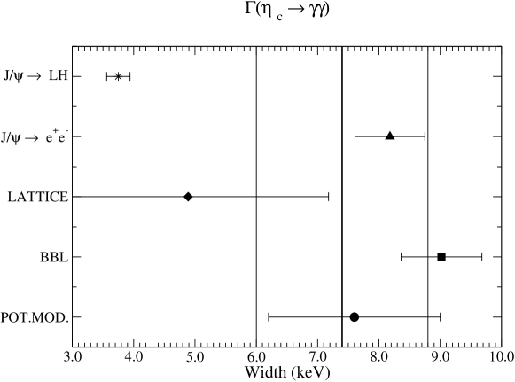
Figure 4: The $\eta_{c}$ two photon width as calculated in this paper using (starting from below) Potential Models results, BBL model with input from $J/\psi$ decay data, Lattice evaluation of $G_{1}$ and $F_{1}$ factors, Singlet picture with $G_{1}$ obtained from $J/\psi\to e^{+}e^{-}$ and $J/\psi\to LH$ processes respectively. The scale has been enhanced with respect to fig. 2 to evidentiate the difference between various theoretical results.

6 Conclusions

The $\Gamma(\eta_{c}\to\gamma\gamma)$ decay width prediction of the potential models considered gives the value $7.6\pm 1.5\textrm{ keV}$ which is consistent with the individual measurements and the world average[23]. The Coulombic model is in agreement with predictions from other models, and gives for the $\eta_{b}\to\gamma\gamma$ decay width the estimate $0.50\pm 0.03\textrm{ keV. }$ Predictions of the BBL model for the $\eta_{c}\to\gamma\gamma$ decay width are consistent with the experimental measurements, for both the long distance terms $G_{1}$ and $F_{1}$ extracted from the $J/\psi$ experimental decay widths and the one evaluated from lattice calculations.

Acnkowledgments

G. P. acknowledges partial support from EC Contract TMR98-0169.

References

-
[1]
A. Böhrer, Bottom Production in Two Photon
Collisions at LEP, DIS01, Bologna, Italy (2001), Proceedings Edi. by
G. Bruni, G. Iacobucci, R. Nania, World Sci., Singapore, 2001;
hep-ex/0106020;
ALEPH Collaboration, Search for in collisions at LEP2 CERN-EP/2002-009; hep-ex/0202011. -
[2]
J. J. Aubert et al., Phys. Rev. Lett. 33 (1974) 1404;
J. E. Augustin et al., Phys. Rev. Lett. 33 (1974) 1406;
G. S. Abrams et al., Phys. Rev. Lett. 33 (1974) 1454. - [3] T. A. Armstrong et al., E760 Collaboration, Phys. Rev. Lett. 70 (1993) 2988.
- [4] A. K. Grant, J. L. Rosner and E. Rynes; Phys. Rev. D 47 (1993) 1981.
- [5] P.L. Franzini, Juliet Lee–Franzini and P.L. Franzini, “Fine structure of the P states in quarkonium and the spin dependent potential ”, LNF-(P).
-
[6]
J.Z. Bai et al., Phys. Lett. B 355 (1995) 374;
S.Y. Hsueh and S. Palestini; Phys. Rev. D 45 (1992) 2181. -
[7]
A. M. Boyarski et al., Phys. Rev. Lett. 34 (1975) 1357;
R. Baldini–Celio et al., Phys. Lett. B 58 (1975) 471;
B. Esposito et al., Nuovo Cimento Lett. 14 (1975) 73;
R. Brandelik et al., Z. Phys. C1 (1979) 233. - [8] G.T. Bodwin, E. Braaten and G.P. Lepage, Phys. Rev. D 51 (1995) 1125.
- [9] M.R. Pennington, Nucl. Phys. B (Proc. Suppl.) 82 (2000) 291.
- [10] A. Czarnecki and K. Melnikov, Phys. Lett. B 519 (2001) 212.
- [11] T. Himel et al., Phys. Rev. Lett. 45 (1980) 1146.
- [12] R. Partridge et al., Phys. Rev. Lett. 45 (1980) 1150.
- [13] G. Brandenburg et al., Phys. Rev. Lett. 85 (2000) 3095.
- [14] The AMY collaboration, M. Shirai et al., Phys. Lett. B 424 (1998) 405.
- [15] The L3 Collaboration, M. Acciarri et al., Phys. Lett. B 461 (1999) 155.
- [16] T. A. Armstrong et al., E760 Collaboration, Phys. Rev. D 52 (1995) 4839.
- [17] H. Albrecht et al., Phys. Lett. B 338 (1994) 390.
- [18] D. Morgan, M. R. Pennington and M. R. Whalley, J. Phys. G: Nucl. Part. Phys. 20 (1994) A1-A147.
- [19] L3 Collaboration, Phys. Lett. B 318 (1993) 575.
- [20] CLEO Collaboration, W. Y Chen et al., Phys. Lett. B 243 (1990) 169.
- [21] TPC/2 Collaboration, Phys. Rev. Lett. 60 (1988) 2355.
- [22] C. Berger et al., Phys. Lett. B 167 (1986) 120.
-
[23]
Review of Particle Properties, D.E. Groom et al.,
Euro. Phys. Journ. C15 (2000) 1;
http://pdg.lbl.gov/. - [24] R.Van Royen and V.Weisskopf, Nuovo Cimento 50A (1967) 617.
- [25] R. Barbieri, G. Curci, E. d’Emilio and R. Remiddi Nucl. Phys. B 154 (1979) 535.
- [26] P. Mackenzie and G. Lepage, Phys. Rev. Lett. 47 (1981) 1244.
- [27] E. Eichten, K. Gottfried, T. Kinoshita, K. D. Lane and T. M. Yan, Phys. Rev. D 21 (1980) 203.
- [28] E. Eichten and F. Feinberg, Phys. Rev. D 23 (1981) 2724.
-
[29]
W.A. Bardeen, A.J. Buras, D.W. Duke and T. Muta, Phys. Rev. D
18 (1978) 3998;
W.J. Marciano, Phys. Rev. D 29 (1984) 580. - [30] J.L. Richardson, Phys. Lett. B 82 (1979) 272.
-
[31]
J. H. Kühn and S. Ono, Zeit. Phys. C21 (1984) 385;
K. Igi and S. Ono, Phys. Rev. D 33 (1986) 3349. - [32] W. Buchmuller and S. H. H. Tye, Phys. Rev. D 24 (1981) 132.
- [33] N. Fabiano, A. Grau and G. Pancheri, Phys. Rev. D 50 (1994) 3173; Nuovo Cimento A, Vol 107 (1994).
-
[34]
V.S. Fadin, V.A. Khoze, JETP Lett. 46 (1987) 525;
V.S. Fadin, V.A. Khoze, Yad. Fiz. 48 (1988) 487. - [35] A. Böhrer, hep-ph/0110030, Talk presented at the International Conference on The Structure and Interactions of the Photon “Photon 2001”, September 2001, Ascona, Switzerland.
- [36] G.A. Schuler, F.A. Berends and R. van Gulik, Nucl. Phys. B 523 (1998) 423.
- [37] N. Fabiano, in preparation.
- [38] G.T. Bodwin, D.K. Sinclair and S. Kim, Int. J. Mod. Phys. A 12 (1997) 4019.
- [39] K.K. Seth, Nucl. Phys. B (Proc. Suppl.) 71 (1999) 413.