FERMILAB-Pub-02/066-T

nuhep-exp/2002-01

hep-ph/0204208

Neutrino Oscillations with a Proton Driver Upgrade and an Off-Axis Detector: A Case Study

Gabriela Barenboim, André de Gouvêa,

Theoretical Physics Division, Fermilab
P.O. Box 500, Batavia, IL 60510, USA

Michał Szleper, and Mayda Velasco

Northwestern University
Department of Physics & Astronomy
2145 Sheridan Rd, Evanston, IL 60208, USA

We study the physics capabilities of the NuMI beamline with an off-axis highly-segmented iron scintillator detector and with the inclusion of the currently under study proton driver upgrade. We focus on the prospects for the experimental determination of the remaining neutrino oscillation parameters, assuming different outcomes for experiments under way or in preparation. An optimization of the beam conditions and detector location for the detection of the $\nu_{\mu}\rightarrow\nu_{e}$-transitions is discussed. Different physics scenarios were considered, depending on the actual solution of the solar neutrino puzzle. If KamLAND measures $\Delta m^{2}_{\odot}$, we find it possible to measure both $|U_{e3}|^{2}$ and the CP violating phase $\delta$ within a viable exposure time, assuming a realistic detector and a complete data analysis. Exposure to both neutrino and antineutrino beams is necessary. We can, in addition, shed light on $\Delta m^{2}_{\odot}$ if its value is at the upper limit of KamLAND sensitivity (i.e., the precise value of $\Delta m^{2}_{\odot}$ remains unknown even after KamLAND). If the solar neutrino solution is not in the LMA region, we can measure $|U_{e3}|^{2}$ and determine the neutrino mass hierarchy. The existence of the proton driver is vital for the feasibility of most of these measurements.

1 Introduction

There is hope that the reconstruction of the neutrino mass matrix will shed light on some of the most relevant open questions faced by high energy physics today, including the origin of the neutrino mass, the flavor-puzzle, and the origin of the asymmetry between matter and antimatter, among others.

In order to start tackling these issues, “precision measurements” of the neutrino parameters are required: simply knowing that the neutrino masses are tiny is not enough. Knowing that there are three non degenerate massive neutrinos is also not enough to prove that there is CP violation in the lepton sector, although it would be rather surprising if it turned out otherwise. Forthcoming neutrino experiments, therefore, have to be designed not simply to test the oscillation hypothesis, but also to perform precise measurements of the oscillation parameters.

We currently know that there are (at least) three neutrino “flavors” – the electron, the muon and the tau neutrinos – and the current neutrino oscillation data strongly suggest that the flavor eigenstates differ from the mass eigenstates and therefore the neutrinos can mix. Furthermore, the atmospheric, solar and reactor data point to two hierarchically different mass-squared differences plus a small “connecting angle,” such that, to good approximation, both the atmospheric and solar neutrino puzzles can be solved by assuming $\nu_{\mu}\leftrightarrow\nu_{\tau}$-oscillations and $\nu_{e}\leftrightarrow\nu_{\rm other}$-oscillations, respectively. Forthcoming results from solar, atmospheric, accelerator, and reactor neutrino oscillation experiments will measure the size of the mass-squared difference and mixing angle that drive the solar neutrino oscillations with good precision and the mass-squared difference and the mixing angle involved in the atmospheric oscillation to about 10% [1] (and there should be direct confirmation that muon neutrinos oscillate to tau neutrinos by direct observation of a tau appearance [2]). Furthermore, we will also definitively open (or close) the door to extra new physics in the neutrino sector by confirming (or not) the LSND anomaly [3] with MiniBooNE data [4].

In addition, some non-oscillation neutrino experiments are aiming at determining the absolute value of the neutrino masses using direct searches [5] and the nature of the neutrino mass: are they Majorana or Dirac particles? [6]. The knowledge of the neutrino mass is important to decide whether neutrinos contribute significantly to the total energy of the Universe.

In view of the above results and the ongoing experimental programs, the ultimate goal for the next generation of neutrino experiments should be to test CP violation in the neutrino sector, if the parameters of the solar neutrino solution allow such a determination. One way to achieve this goal is to devise experiments that:

• are sensitive to the sub-dominant $\nu_{\mu}\rightarrow\nu_{e}$ channel for the atmospheric $L/E_{\nu}$, and can measure $|U_{e3}|$ from both $\nu_{\mu}\rightarrow\nu_{e}$ and $\bar{\nu}_{\mu}\rightarrow\bar{\nu}_{e}$ transitions;

• are capable of determining the neutrino mass pattern from matter effects;

• ultimately, can test CP invariance in the leptonic sector.

Such experiments require, in general, relatively intense and mono-energetic beams. As first suggested in [7], this could be achieved with off-axis neutrino beams.

The literature contains a significant amount of work [8, 9] which discusses the potential of generic “super-beams,” with neutrino energies ranging from 1 to 50 GeV and baselines spanning from 200 to 7000 kilometers. Low energy neutrino beams have also been studied [10]. In this work, we explore which of the questions above can be addressed by using the NuMI beam line with a new proton driver and the construction of an off-axis detector. We will concentrate exclusively on what one may hope to learn by looking for $\nu_{\mu}\rightarrow\nu_{e}$ appearance in a highly segmented iron-scintillator detector. We will conclude, in agreement with some of these previous works, that intense beams can significantly improve our knowledge of the neutrino oscillation parameters, including (depending on the solar solution) some sensitivity to a CP violating phase. However, the ultimate sensitivity to some of the neutrino parameters, in particular the CP violating phase, will require the purity and intensity of neutrino factory beams [11].

The paper is organized as follows. First, we briefly review the neutrino mixing matrix and oscillation probabilities, and describe the current knowledge of neutrino masses and mixing angles. In Sec. 3, we describe the off-axis neutrino beam, and discuss where an off-axis detector should be located in order to maximize its physics capabilities. In Sec. 4, we describe in detail the detector we will be considering, and discuss reconstruction efficiencies and strategies for reducing the number of background events. In Sec. 5, we discuss the physics capabilities of such a setup, for different values of the solar mass-squared difference. We find that while some information can be obtained from a “neutrino” beam, it is imperative to run with an “antineutrino” beam as well. Furthermore, in order to extract more “exciting” physics (such as CP-violation) out of the experiment, a new intense proton source and a large detector are required. In Sec. 6 we summarize our results and compare our findings with similar studies at different beamlines.

2 Neutrino Mixing and Oscillations

The presence of non-zero masses for the light neutrinos introduces a leptonic mixing matrix, $U$, analogous to the well known CKM quark mixing matrix, and which in general is not expected to be diagonal. The matrix $U$ connects the neutrino flavor eigenstates with the mass eigenstates:

$$|\nu_{\alpha}\rangle=\sum_{i}U_{\alpha i}|\nu_{i}\rangle,$$ (2.1)

where $\alpha$ denotes the active neutrino flavors, $e,\ \mu$ or $\tau$, while $i$ runs over the mass eigenstates. It is “traditional” to define the mixing angles $\theta_{12,13,23}$ in the following way:

$$\tan^{2}\theta_{12}\equiv\frac{|U_{e2}|^{2}}{|U_{e1}|^{2}},~{}~{}~{}\tan^{2}\theta_{23}\equiv\frac{|U_{\mu 3}|^{2}}{|U_{\tau 3}|^{2}},~{}~{}~{}\sin^{2}\theta_{13}\equiv|U_{e3}|^{2},$$ (2.2)

while

$$\Im(U_{e2}^{*}U_{e3}U_{\mu 2}U_{\mu 3}^{*})\equiv\sin\theta_{12}\cos\theta_{12}\sin\theta_{23}\cos\theta_{23}\sin\theta_{13}\cos^{2}\theta_{13}\sin\delta,$$ (2.3)

defines the CP-odd phase $\delta$. For Majorana neutrinos, $U$ contains two further multiplicative phase factors, but these are invisible to oscillation phenomena.

In order to relate the mixing angles and mass-squared differences to the parameters constrained by experiments, it is convenient to define the neutrino masses such that $m_{1}^{2}<m^{2}_{2}$ with $\Delta m^{2}_{12}<|\Delta m^{2}_{13,23}|$ (the data, in fact, point to $\Delta m^{2}_{12}\ll|\Delta m^{2}_{13,23}|$). With this definition, the “solar angle” $\theta_{\odot}\simeq\theta_{12}$, while the “atmospheric angle” $\theta_{\rm atm}\simeq\theta_{23}$. Furthermore, reactor experiments constrain $|U_{e3}|^{2}$. The solar mass-squared difference $\Delta m^{2}_{\odot}=\Delta m^{2}_{12}$, while the atmospheric mass-squared difference is $\Delta m^{2}_{\rm atm}=|\Delta m^{2}_{13}|\simeq|\Delta m^{2}_{23}|$. It is important to note that $m_{3}^{2}$ can be either larger or smaller than $m_{1}^{2},m_{2}^{2}$.

The oscillation probability $P(\nu_{\alpha}\rightarrow\nu_{\beta})$ is given by the absolute square of the overlap of the observed flavor state, $|\nu_{\beta}\rangle$, with the time-evolved initially-produced flavor state, $|\nu_{\alpha}\rangle$. In vacuum, it yields the well-known result:

$$\begin{array}[]{rl}P(\nu_{\alpha}\rightarrow\nu_{\beta})=&\left|\langle\nu_{\beta}|e^{-iH_{0}L}|\nu_{\alpha}\rangle\right|^{2}=\sum_{i,j}U_{\alpha i}U^{*}_{\beta i}U^{*}_{\alpha j}U_{\beta j}e^{-i\Delta m^{2}_{ij}L/2E}\\[7.22743pt] =&P_{\rm CP-even}(\nu_{\alpha}\rightarrow\nu_{\beta})+P_{\rm CP-odd}(\nu_{\alpha}\rightarrow\nu_{\beta})\;.\\[7.22743pt] \end{array}$$ (2.4)

The CP-even and CP-odd contributions are

$$\begin{array}[]{rl}P_{\rm CP-even}(\nu_{\alpha}\rightarrow\nu_{\beta})=&P_{\rm CP-even}(\bar{\nu}_{\alpha}\rightarrow\bar{\nu}_{\beta})\\[7.22743pt] =&\delta_{\alpha\beta}-4\sum_{i>j}\ Re\ (U_{\alpha i}U^{*}_{\beta i}U^{*}_{\alpha j}U_{\beta j})\sin^{2}({{\Delta m^{2}_{ij}L}\over{4E}}),\\[7.22743pt] P_{\rm CP-odd}(\nu_{\alpha}\rightarrow\nu_{\beta})=&-P_{\rm CP-odd}(\bar{\nu}_{\alpha}\rightarrow\bar{\nu}_{\beta})\\[7.22743pt] =&2\sum_{i>j}\ Im\ (U_{\alpha i}U^{*}_{\beta i}U^{*}_{\alpha j}U_{\beta j})\sin({{\Delta m^{2}_{ij}L}\over{2E}}),\\[7.22743pt] \end{array}$$ (2.5)

such that,

$$P(\bar{\nu}_{\alpha}\to\bar{\nu}_{\beta})=P(\nu_{\beta}\to\nu_{\alpha})=P_{\rm CP-even}(\nu_{\alpha}\rightarrow\nu_{\beta})-P_{\rm CP-odd}(\nu_{\alpha}\rightarrow\nu_{\beta}),$$ (2.6)

where, by CPT invariance, $P(\nu_{\alpha}\to\nu_{\beta})=P(\bar{\nu}_{\beta}\to\bar{\nu}_{\alpha})$. In vacuum the CP-even and CP-odd contributions are even and odd, respectively, under time reversal: $\alpha\leftrightarrow\beta$.

If the neutrinos propagate in ordinary matter, these expressions are modified. The propagation of neutrinos through matter is very well described by the evolution equation

$$i{d\nu_{\alpha}\over dt}=\sum_{\beta}\left[\left(\sum_{j}U_{\alpha j}U_{\beta j}^{*}{m_{j}^{2}\over 2E_{\nu}}\right)+{A\over 2E_{\nu}}\delta_{\alpha e}\delta_{\beta e}\right]\nu_{\beta}\,,$$ (2.7)

where $A/(2E_{\nu})$ is the amplitude for coherent forward charged-current scattering of $\nu_{e}$ on electrons,

$$A=2\sqrt{2}G_{F}N_{e}E_{\nu}=1.52\times 10^{-4}~{}{\rm eV^{2}}Y_{e}\rho({\rm\,g/cm^{3}})E({\rm\,GeV}).\,$$ (2.8)

For antineutrinos, $A$ is replaced with $-A$, and $U$ with $U^{*}$. Here $Y_{e}$ is the electron fraction and $\rho(t)$ is the matter density. For neutrino trajectories through the earth’s crust, the density is typically of order 3 g/cm³, and $Y_{e}\simeq 0.5$. For propagation through matter of constant density, the transition probabilities can be written in the form Eq. (2.5) if the mass-squared differences and mixing angles are replaced by the corresponding “matter” counterparts. Long baseline neutrino experiments are sensitive to matter effects, and the magnitude of the effect strongly depends on the baseline length and neutrino energy. Some examples are depicted in Figs. 1 and 2.

Figure 1: Transition probabilities for neutrinos (green, top curve) and antineutrinos (blue, bottom curve) in matter and vacuum (red, middle curve) as function of the energy for L= 735 km, $\Delta m^{2}_{13}=3\cdot 10^{-3}~{}{\mbox{eV}}^{2}$ (normal hierarchy), $\theta_{\rm atm}=\pi/4$, $\Delta m^{2}_{\odot}=1\times 10^{-4}$ eV², $\theta_{\odot}=\pi/6$, $|U_{e3}|^{2}=0.04$, and $\delta=0$.

Figure 2: Transition probabilities for neutrino (green, top curve) and antineutrinos (blue, bottom curve) in matter and vacuum (red, middle curve) for 2 GeV as function of the distance, $\Delta m^{2}_{13}=3\cdot 10^{-3}~{}{\mbox{eV}}^{2}$ (normal hierarchy), $\theta_{\rm atm}=\pi/4$, $\Delta m^{2}_{\odot}=1\times 10^{-4}$ eV², $\theta_{\odot}=\pi/6$, $|U_{e3}|^{2}=0.04$, and $\delta=0$.

There are some unknowns related to the neutrino mass pattern which can be addressed with the “help” of the matter effects. As alluded to before, the current data leave us with two alternatives for the spectrum of the three active neutrino species: a “normal” neutrino mass hierarchy or an “inverted” neutrino mass hierarchy. In the case of a “normal” mass hierarchy, the “solar pair” of states is lighter than $\nu_{3}$, i.e.  $m^{2}_{3}>m^{2}_{2},m^{2}_{1}$. In the case of inverted hierarchy, the states of the solar pair are heavier than $\nu_{3}$, i.e.  $m^{2}_{3}<m^{2}_{2}\simeq m^{2}_{1}$. The key difference between these two hierarchies is then that, in the normal hierarchy, the small $U_{e3}$ admixture of $\nu_{e}$ is in the heaviest state whereas in the inverted hierarchy, this admixture is in the lightest state. The difference between both schemes is parameterized by the sign of $\Delta m^{2}_{13}$. A positive (negative) $\Delta m^{2}_{13}$ will point towards a normal (inverted) hierarchy.

In going from $\nu$ to $\overline{\nu}$, there are matter-induced CP- and CPT- odd effects associated with the change $A\rightarrow-A$. The additional change U $\rightarrow$ U^∗ introduces further effects (this is the “genuine” CP-violation), which are usually sub-leading. Note that the matter effects depend on the interference between the different flavors and on the relative sign between $A$ and $\Delta m^{2}_{13}$. Consequently, the experimental distinction between the propagation of $\nu$ and $\overline{\nu}$ (the sign of $A$) can possibly determine the sign of $\Delta m^{2}_{13}$. Fig. 3 shows the transition probabilities for the two possible choices of the sign of $\Delta m^{2}_{13}$ in the case of $|\Delta m^{2}_{13}|=3\cdot 10^{-3}~{}{\mbox{eV}}^{2}$, $\theta_{\rm atm}=\pi/4$, $\Delta m^{2}_{\odot}=1\times 10^{-7}$ eV², $\theta_{\odot}=\pi/6$, $|U_{e3}|^{2}=0.01$, and $\delta=0$.

Figure 3: $\nu_{\mu}\rightarrow\nu_{e}$ oscillation probability for $\Delta m^{2}_{13}>0$ (solid line) and $\Delta m^{2}_{13}<0$ (dashed line). $|\Delta m^{2}_{13}|=3\cdot 10^{-3}~{}{\mbox{eV}}^{2}$, $\theta_{\rm atm}=\pi/4$, $\Delta m^{2}_{\odot}=1\times 10^{-7}$ eV², $\theta_{\odot}=\pi/6$, $|U_{e3}|^{2}=0.01$, and $\delta=0$.

What is currently known about the oscillation parameters? The atmospheric neutrino puzzle points to a “well determined” mass-squared difference band [12],

$$1.5\cdot 10^{-3}~{}{\mbox{eV}}^{2}\mathrel{\mathchoice{\lower 3.0pt\vbox{\halign{$\m@th\displaystyle\hfill#\hfil$\cr<\crcr\sim\crcr}}}{\lower 3.0pt\vbox{\halign{$\m@th\textstyle\hfill#\hfil$\cr<\crcr\sim\crcr}}}{\lower 3.0pt\vbox{\halign{$\m@th\scriptstyle\hfill#\hfil$\cr<\crcr\sim\crcr}}}{\lower 3.0pt\vbox{\halign{$\m@th\scriptscriptstyle\hfill#\hfil$\cr<\crcr\sim\crcr}}}}\Delta m^{2}_{\rm atm}\mathrel{\mathchoice{\lower 3.0pt\vbox{\halign{$\m@th\displaystyle\hfill#\hfil$\cr<\crcr\sim\crcr}}}{\lower 3.0pt\vbox{\halign{$\m@th\textstyle\hfill#\hfil$\cr<\crcr\sim\crcr}}}{\lower 3.0pt\vbox{\halign{$\m@th\scriptstyle\hfill#\hfil$\cr<\crcr\sim\crcr}}}{\lower 3.0pt\vbox{\halign{$\m@th\scriptscriptstyle\hfill#\hfil$\cr<\crcr\sim\crcr}}}}5\cdot 10^{-3}~{}{\mbox{eV}}^{2}$$ (2.25)

with $\sin^{2}(2\theta_{\rm atm})\mathrel{\mathchoice{\lower 3.0pt\vbox{\halign{$\m@th\displaystyle\hfill#\hfil$\cr>\crcr\sim\crcr}}}{\lower 3.0pt\vbox{\halign{$\m@th\textstyle\hfill#\hfil$\cr>\crcr\sim\crcr}}}{\lower 3.0pt\vbox{\halign{$\m@th\scriptstyle\hfill#\hfil$\cr>\crcr\sim\crcr}}}{\lower 3.0pt\vbox{\halign{$\m@th\scriptscriptstyle\hfill#\hfil$\cr>\crcr\sim\crcr}}}}0.88$, while the solar neutrino puzzle points to many disconnected regions. Loosely speaking, $\Delta m^{2}_{\odot}$ can lie anywhere between $10^{-10}$  eV² and $7\times 10^{-4}$ eV² (the best upper limit is provided by the CHOOZ experiment). Global fits to all data have historically identified the following well-known regions [13]:

• LMA, large mixing angle: $\Delta m_{\odot}^{2}=(1-10)\cdot 10^{-5}$ eV², $\tan^{2}\theta_{\odot}$ = 0.2–5;

• SMA, small mixing angle: $\Delta m_{\odot}^{2}=(4-10)\cdot 10^{-6}$ eV², $\tan^{2}\theta_{\odot}=(1-10)\cdot 10^{-3}$;

• LOW-QVO, large mixing angle, small $\Delta m^{2}_{\odot}$: $\Delta m_{\odot}^{2}=(0.5-2)\cdot 10^{-7}$ eV² , $\tan^{2}\theta_{\odot}$ = 0.1 – 10;

• VO, large mixing, vacuum oscillations: $\Delta m_{\odot}^{2}=(4-6)\cdot 10^{-10}$ eV² and $(6-8)\cdot 10^{-11}$ eV², $\tan^{2}\theta_{\odot}=0.1-3$.

Notice that all the solutions satisfy

$$\Delta m_{\odot}^{2}\ll\Delta m_{\rm atm}^{2}$$ (2.26)

implying that there is indeed a hierarchy between the two distinct mass-squared differences. Current global fits point towards electron neutrino oscillations to active neutrinos (either muon or tau neutrinos) in the LMA region (a small region in the LOW area is also allowed while the SMA and VO regions are strongly disfavored). Although the LMA solution is the most favored, this ambiguity must be removed by identifying the correct solution to the solar neutrino problem. This issue will be addressed by the KamLAND [14] reactor neutrino experiment, which is capable of confirming or excluding, unambiguously, the LMA solution, and precisely measuring the solar oscillation parameter if LMA is indeed correct. However, it is important to remember that if the mass-squared difference driving solar neutrino oscillations lies in the “high-end” of the LMA region, the length of the baseline will be too long and the oscillation peaks will not be resolved experimentally [15, 16]. The positron spectrum will be depleted (proportionally to the solar mixing angle) but will not be distorted as the oscillatory term will average out. In this case, the mass difference will be confined to a region whose lower limit is given by the KamLAND sensitivity and whose upper limit is dictated by the CHOOZ bound. Thus, as this mass-squared difference is an essential input in analyzing long baseline experiments, the capabilities of any future determination should take this possibility into account. Furthermore, a solar mass difference belonging to the upper part of the LMA region will have a strong impact on the oscillation probabilities, as the often neglected sub-dominant oscillations become not that sub-dominant any more.

In order to determine the sensitivity of a given experiment to some parameter, it is imperative to distinguish different scenarios regarding the solar mass difference. We decide to study three different scenarios:

1. KamLAND does not see an oscillation signal, implying that the LOW solution would be correct [15] (or, perhaps one of the disfavored non LMA solutions). In this case, solar driven oscillations become negligible and there is no room for measuring CP violation in the neutrino sector. Nonetheless, one can still attempt to determine $|U_{e3}|^{2}$, and, if a nonzero $|U_{e3}|^{2}$ is observed, determine the neutrino mass hierarchy.

2. KamLAND does provide a precise measurement of the solar mass-squared difference. The determination of the CP violating phase and $|U_{e3}|^{2}$ from a simultaneous fit to both parameters becomes possible.

3. KamLAND sees an overall suppression of the total rate but is not capable of measuring the mass-squared difference. In this case one must attempt to measure not only $|U_{e3}|^{2}$ and $\delta$, but also the solar mass-squared difference. While the overall picture is rather “dirty,” there is no reason to believe that a combined analysis is impossible (after all, for such large $\Delta m^{2}_{\odot}$, there will be no shortage of $\nu_{e}$-induced events!).

3 NuMI Off-Axis Beams

The Neutrinos at the Main Injector (NuMI) [18] tertiary beamline was designed to provide an intense $\nu_{\mu}$ beam to the MINOS experiment [19]. The $\nu_{\mu}(\bar{\nu}_{\mu})$’s are derived from secondary $\pi^{+}(\pi^{-})$ and $K$ beams that are allowed to decay within a 675 m decay tunnel. 120 GeV protons will be extracted from the Main Injector via a single turn extraction ($8.6~{}\mu$s pulse, cycle time $1.9$ s.) and focused downward by 58 mrad, where the proton impinge into a 0.94 m graphite target to produce the secondary hadron ($\pi$, $K$) beams. NuMI is expected to receive $4\times 10^{13}$ protons/pulse.

MINOS is in a cavern of the Soudan mine located at a distance of 735 km from FNAL. The beam is tuned to make the experiment well aligned with respect to the beam axis. Another way of efficiently using this beamline would be to construct detectors located away from the beam axis. The resulting neutrino beam energy spectra at the different locations can be predicted from energy and momentum conservation in the $\pi$ decay process:

$$E_{\nu}=\frac{m^{2}_{\pi}-m^{2}_{\mu}}{2(E_{\pi}-p_{\pi}\cos\theta_{\nu})}=\frac{0.004~{}\rm GeV}{(E_{\pi}-p_{\pi}\cos\theta_{\nu})},$$ (3.27)

where $m_{\pi}$ and $m_{\mu}$ are the rest masses, $E_{\pi}$ and $p_{\pi}$ are the pion energy and momentum, and $\cos\theta_{\nu}$ is the angle at which the neutrino is emitted with respect to the pion direction. The maximum angle in the lab frame relative to the pion direction is related to the neutrino energy by:

$$\theta^{max}_{\nu}=\frac{(30+\Delta_{T})~{}\rm MeV}{E_{\nu}},$$ (3.28)

where 30 MeV is the neutrino momentum in the rest frame of the pion, while $\Delta_{T}$ takes into account the nonzero transverse momentum of the decaying $\pi$. As shown in Fig. 4(a), if $\theta_{\nu}\simeq 0$ the neutrino energy is proportional to the pion energy ($E_{\nu}=0.44E_{\pi}$), while at an off-axis location ($\theta_{\nu}\neq 0$) there is a maximum neutrino energy which is independent of the energy of the parent pion. Therefore, the off-axis configuration allows one to use a fraction of the “total” beam that is characterized by having lower $E_{\nu}$. The maximum flux for a fixed $E_{\nu}$ will be obtained when operating close to the corresponding $\theta^{max}_{\nu}$, see Fig. 4(b). The lower energy neutrinos provided by NuMI off-axis beams are highly desirable because they allow beams which are more suitable for oscillation studies, given the current knowledge of oscillation parameters (see Table 1), while still having large enough energy and baseline length to be sensitive to matter effects (see Sec. 2).

Table 1: The first transition for $\nu_{\mu}\rightarrow\nu_{X}$ occurs when $1.27|\Delta m^{2}_{13}|(L/E_{\nu})=\pi/2$. Note that baselines much greater than 900 km are not allowed in our set up, because they would require “levitating” detectors.

$\Delta m^{2}_{13}(\rm eV^{2})$	0.002	0.0025	0.003
Energy (GeV)	1.5 (2)	1.5 (2)	1.5 (2)
Length (km)	928 (1236)	742 (989)	618 (824)

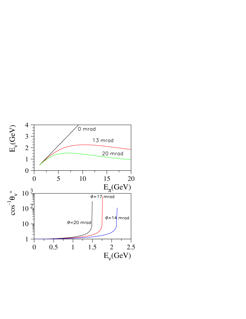
Figure 4: top – allowed $E_{\nu}$ values for several $\theta_{\nu}$ values. bottom – shows $1/\cos\theta^{*}_{\nu}$ that is proportional to the neutrino flux. $\cos\theta^{*}_{\nu}=\sqrt{1-\frac{E^{2}_{\nu}}{E^{*2}_{\nu}}\tan^{2}\theta_{\nu}}$ is the $\nu$ production angle in the rest frame of the $\pi$.

Two toroidal magnetic horns sign and momentum-select the secondary beam. The horns are movable allowing one to obtain different neutrino energy spectra. For example, Fig. 5 depicts the expected energy spectrum at different location for the low energy (horns 10 m apart) and the medium energy (horns 27 m apart) horn configurations. As shown, the off-axis beams are characterized by having a narrow and well-defined energy distribution with fluxes higher than the corresponding on-axis energy. In addition, the harmful high energy tail of the on-axis beams is not present, as expected from energy and momentum conservation, Eq. (3.27). All these distributions are calculated using the GNuMI GEANT based Monte Carlo [20], and include the full beamline, target and decay pipe description.

In addition to the off-axis beam properties described in Fig. 4, there are two basic facts that should be kept in mind when optimizing the beam configuration: (1) the beam flux decreases as the baseline increases, and (2) the beam flux decreases as the off-axis angle increases. Here we have performed two types of detector location optimization.

The first one is referred to as the naive beam optimization, where we optimize the detector location such that $1.27|\Delta m^{2}_{13}|L/E_{\nu}=\pi/2$. That is, for a given $|\Delta m^{2}_{13}|$ and $L$ we have set $\theta_{exp}\simeq\theta^{max}_{\nu}$ to get the corresponding $E_{\nu}$ to be the maximum energy, which by definition will also correspond to the point of maximum flux. For example, $30~{}\rm MeV/2.25~{}\rm GeV\simeq 12~{}\rm km/900~{}\rm km\simeq 0.013$ mrad and $30~{}\rm MeV/1.75~{}\rm GeV\simeq 12.5~{}\rm km/735~{}\rm km\simeq 0.017$ mrad. These results are depicted in Figs. 6 and 7 for $\Delta m^{2}_{13}=0.003$ and 0.0025 eV², respectively.

From this exercise we learn that, if we are interested in configurations with small $\Delta m^{2}_{13}$, very small energies will be required if the baseline is short. As a consequence, large angles are required, say $\leq 20$ mrad, and the lower acceptance in the medium energy beam for pions with wide angles becomes a limitation. This can be compensated for by increasing the baseline, therefore increasing the required energy and lowering the required angle. More important is the fact that, with the medium energy beam, there is a higher overall flux between 1.5 and 3 GeV, and a lower high energy tail than with a low energy beam, if one operates with angles that are smaller than $\sim$15 mrad. These two facts make the medium energy beam preferable.

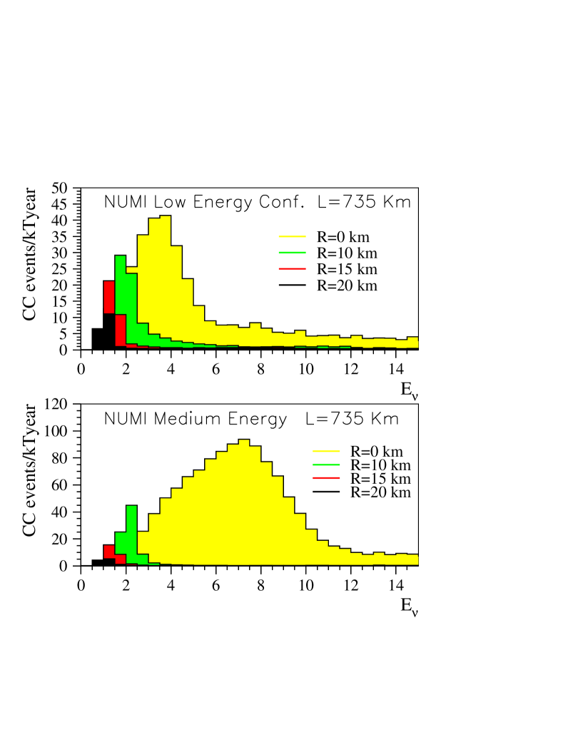
Figure 5: On and off-axis beams for the low and medium energy NuMI horns configuration. A full beam simulation was made using the GEANT based GNuMI Monte Carlo.

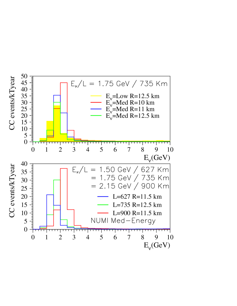
Figure 6: Beam optimization for a fixed value of $L/E_{\nu}$ given $\Delta m^{2}_{13}\simeq 0.003~{}\rm eV^{2}$. The medium energy configuration gives a higher event yield and cleaner beam conditions.

Figure 7: Beam optimization for a fixed value of $L/E_{\nu}$ given $\Delta m^{2}_{13}\simeq 0.0025~{}\rm eV^{2}$. The low (medium) energy configuration gives a higher event yield at 735(900) km.

The off-axis reduction of the high energy tail of the medium energy beam is depicted in Fig. 7. There are two reasons for this: (1) the transverse momentum of the pions is smaller for the medium energy configuration making $\Delta^{medium}_{T}<\Delta^{low}_{T}$, and (2) the mean energy of the kaons in the medium energy beam is higher producing neutrinos that are of higher energy and therefore less harmful to the analysis, see Fig. 8.

In order to determine how well different $\nu_{\mu}$ transitions can be measured, all possible backgrounds have to be taken into account. Due to the short beam pulse duration and well defined repetition rate of the resulting neutrino beamline, it is possible to reject the cosmic ray background even if the detector considered here is located at the surface. On the other hand, beam neutrinos induce other background events, which must be dealt with. The flavor composition of the “neutrino beam” is depicted in Fig. 9. For the neutral current (NC) background calculations, all neutrino flavors contribute. For $\nu_{\mu}\rightarrow\nu_{e}$-transitions, the inherent $\nu_{e}$ in the beam contributes with further (irreducible) background events. Assuming that we can not detect the sign of the outgoing lepton in charged current (CC) events, the relevant quantity is the ratio of $(\nu_{e}+\bar{\nu}_{e})/(\nu_{\mu}+\bar{\nu}_{\mu})$, which is depicted in Fig. 10. The $\nu_{\tau}$ CC cross section for $E_{\nu}<5$ GeV is zero [21], and therefore not relevant for the off-axis beam under consideration.

Studies of matter effects and CP violation require the comparison of $\nu_{\mu}$ and $\bar{\nu}_{\mu}$ oscillations. An “anti-neutrino beam” can be produced by reversing the polarity of the horns. This beam’s flavor composition and $(\nu_{e}+\bar{\nu}_{e})/(\nu_{\mu}+\bar{\nu}_{\mu})$ are also depicted in Figs. 9 and 10. The beam related background is at the same level for both horn polarities, but the CC event rate is at least three times smaller for $\bar{\nu}_{\mu}$ with energies above 2.5  GeV and five times smaller for the lower neutrino energies. As shown in Fig. 11, this is mostly caused by the cross section difference, and not by the $\pi^{+}$, $\pi^{-}$ production rate.

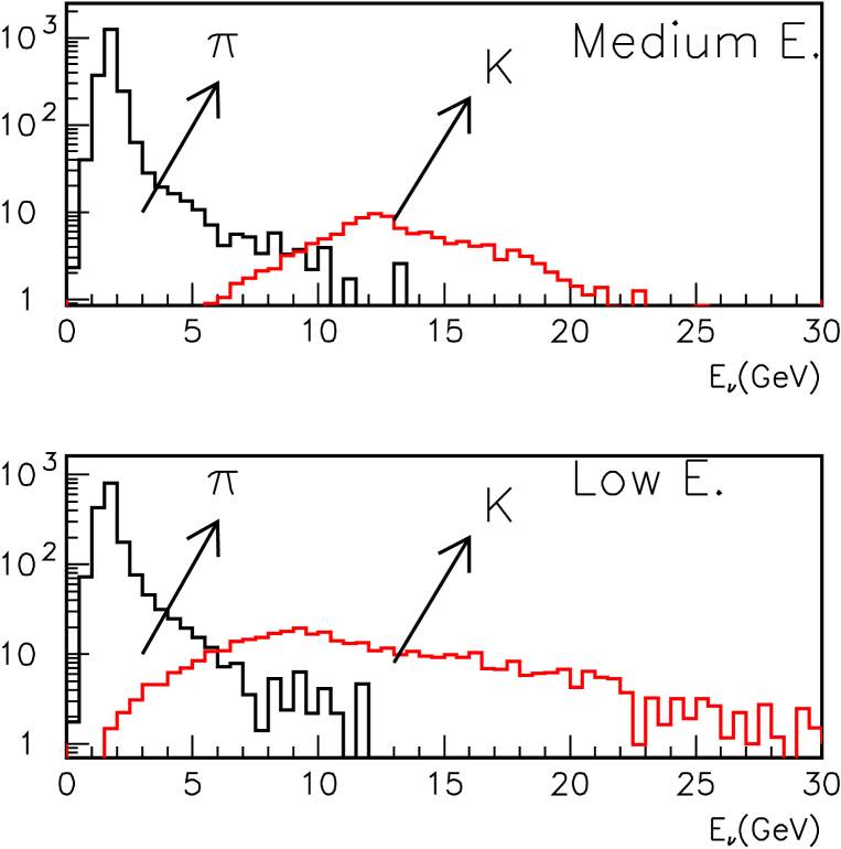
Figure 8: Contribution from $\pi$ and kaons to the beam composition for off-axis beams in the medium and low energy beam horn configuration.

In the second type of beam optimization, we look at locations with smaller $\theta_{\nu}$. These locations are characterized by having a broader energy spectrum and a higher overall flux for neutrinos with energies below 3 GeV. This is illustrated in Fig. 6(top), where we show the energy distributions at several radii and at a fixed length. Clearly, for a detector located at a radius of 10 km (13 mrad) instead of 12.5 km (17 mrad), we have at least two times more flux between 1.5 and 3 GeV. These broader energy beams are suitable for a wider range of $\Delta m^{2}_{13}$, but how useful they are for $\nu_{\mu}\to\nu_{e}$ appearance experiments will depend on how well one can keep the NC background under control. Therefore, in order to conclude how much better these larger $\theta_{\nu}$ off-axis experiments really are requires a full evaluation of the signal and backgrounds with a realistic detector simulation and reconstruction. We have performed such analysis and the details are given in Sec. 4. Here we will just summarize the results by evaluating a figure-of-merit (FOM) at each location for $\nu_{\mu}\to\nu_{e}$ in the case of full mixing and $|U_{e3}|^{2}=0.01$. We defined the FOM as $S/\sqrt{S+B}$, where $S$ and $B$ are the signal and background events that survive all the cuts in the reconstruction. As depicted in Fig. 12, off-axis experiments with angles between $10\leq\theta_{\nu}\leq 13$ mrad from the axis have a high FOM for all values of $\Delta m^{2}_{13}$. The high FOM is not only due to the characteristics of the beam and oscillation probabilities (see Fig. 13), but also due to the fact that in all cases we can keep the NC background at the 0.5% level, while the reconstruction efficiency is about 40%. If we look in detail at the case of $\Delta m^{2}_{13}=0.003~{}\rm eV^{2}$, we can see that the naive beam tune performed at 735 km cannot compete with smaller $\theta_{\nu}$ locations at the same baseline. This is not true for the naive beam tune performed at 900 km, where at that location $\theta_{\nu}$ is already small enough to give us a high integrated flux. We can still obtain a 20% increase in the FOM by reducing the baseline to 735 km and $\theta_{\nu}$ to 10 mrad, but at the moment this is not particularly relevant, given the current lack of knowledge of neutrino oscillations parameters. For example, in Fig. 13 we have assumed a normal neutrino mass hierarchy, and an inverted hierarchy would significantly modify what the optimal conditions are. Furthermore, the inclusion of (potentially significant) solar oscillations and CP-violating effects further cloud the picture. Nonetheless, the FOM is flat enough that any “reasonable” choice of baseline and opening angle should be “close” to optimal. We, therefore, will do all our analyses for a baseline of 900 km and at a radius of 11.5 km.

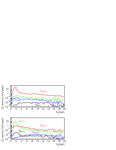
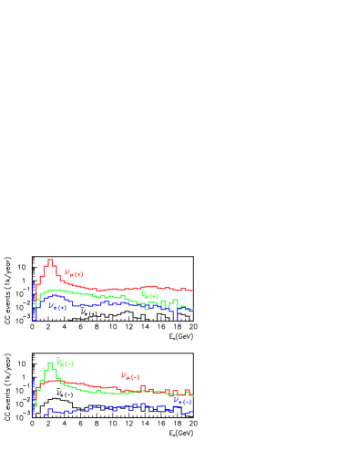
Figure 9: Beam composition for positive (+) and negative (-) horn currents. left: for the a low energy configuration at $L=735$ km and $R=10$ km. right: for the a medium energy configuration at $L=900$ km and $R=12$ km.

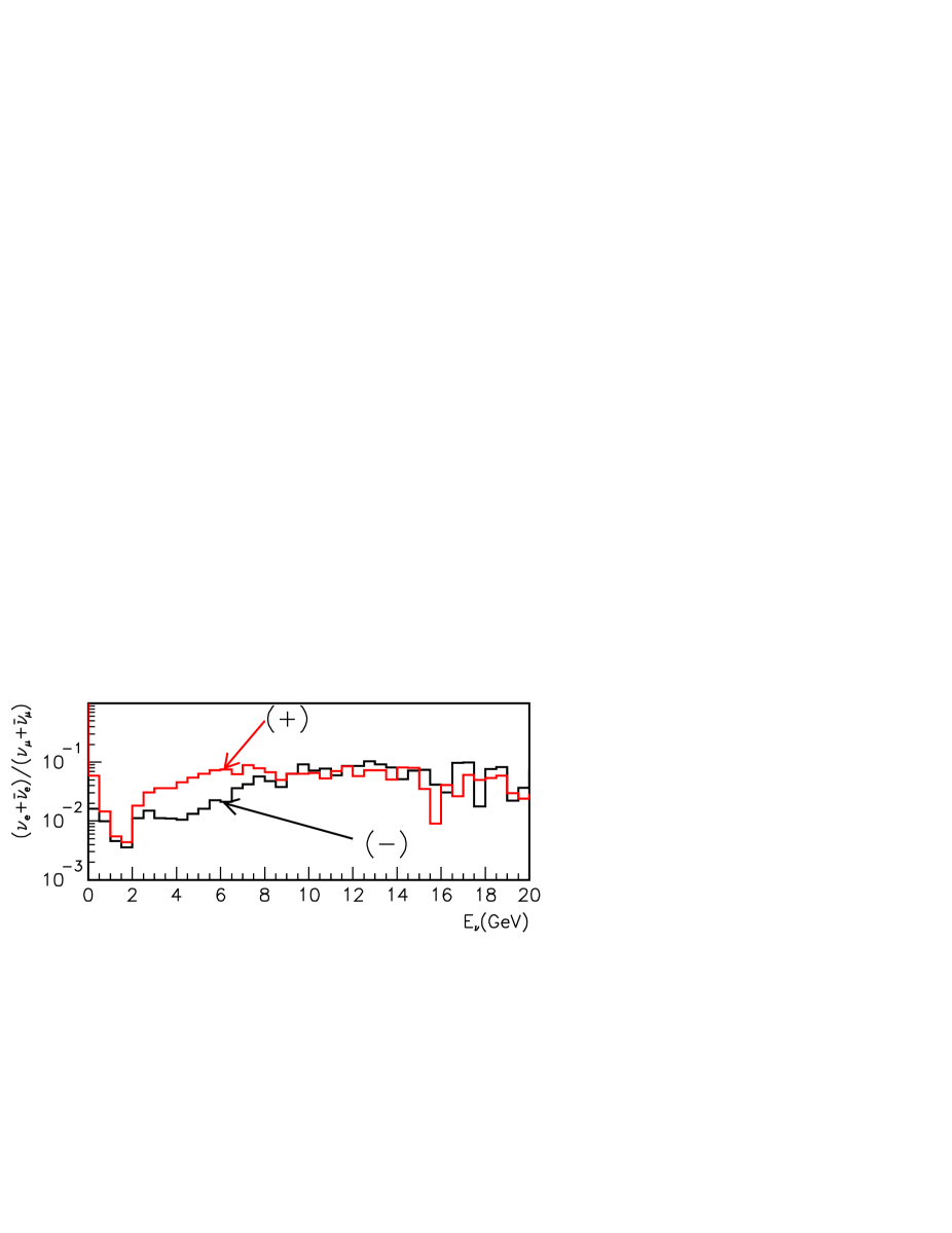
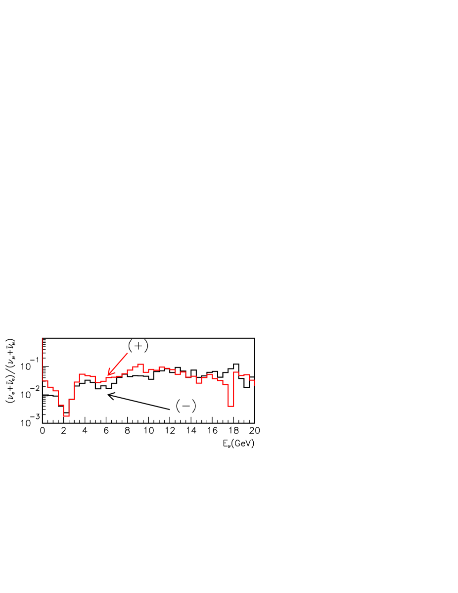
Figure 10: The $(\nu_{e}+\bar{\nu}_{e})/(\nu_{\mu}+\bar{\nu}_{\mu})$ does not degrade when going from (+) to (-) polarity in the horns. In both cases, the $\nu_{e}+\bar{\nu}_{e}$ fraction of the beam is below 0.5% in the signal region. top – is for a low energy configuration at $L=735$ km and $R=10$ km. bottom: is for a medium energy configuration at $L=900$ km and $R=12$ km.

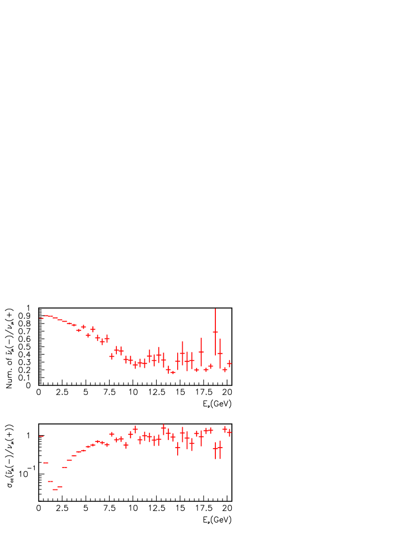
Figure 11: Comparison between the neutrino and anti-neutrino beams for charge current events. As shown, the lower rate is due to the cross section and not to the $\pi$ production rate.

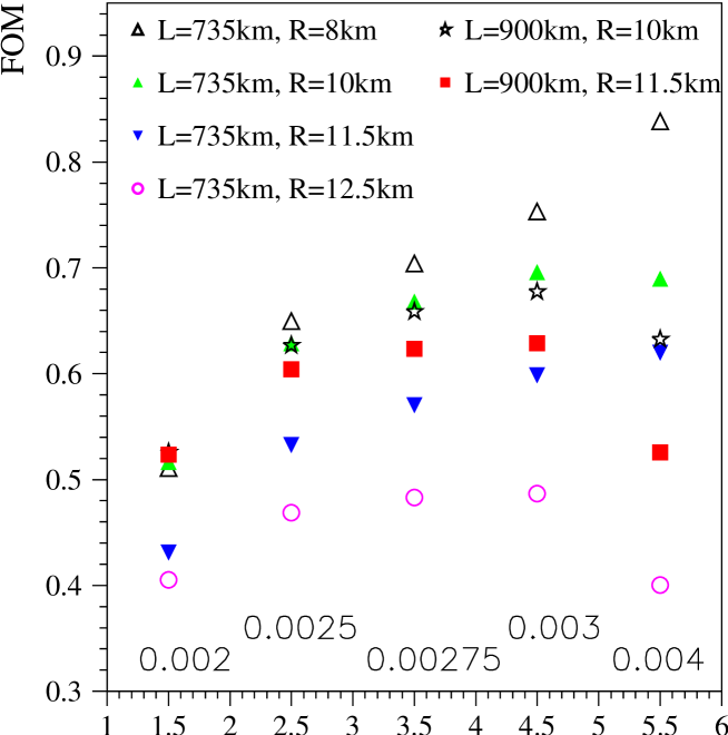
Figure 12: FOM for $\nu_{\mu}\to\nu_{e}$ appearance for different values of $\Delta m^{2}_{13}$ in the case of full mixing and $|U_{e3}|^{2}=0.01$ for different baselines and $\theta_{\nu}$, but with the same detector and reconstruction criteria. We only select events with visible energy between 1 and 3 GeV. If this highly segmented detector were at the MINOS location and $\Delta m^{2}_{13}$ were $0.003$ eV², the corresponding FOM would be 0.54. This is to be compared to the FOM for the MINOS detector that is only 0.39 [22]. This means, that if we ignore the background uncertainty, about half of the gain in sensitivity is due to the location and the other half to the detector.

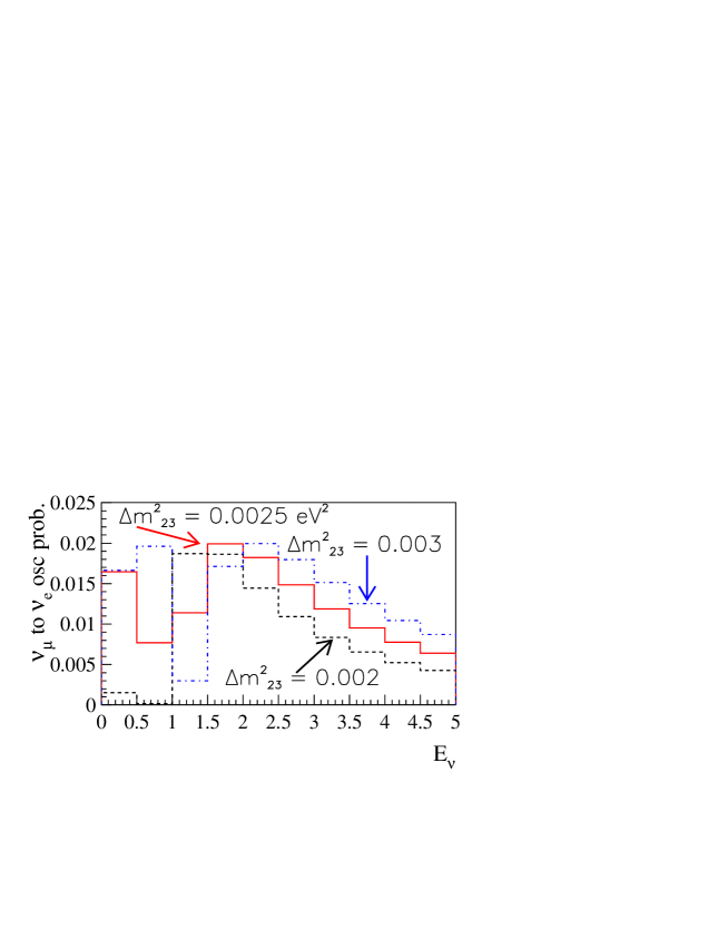
Figure 13: Transition probability for $\nu_{\mu}\to\nu_{e}$ in the case of maximal atmospheric mixing and $|U_{e3}|^{2}=0.01$, for different values of $\Delta m^{2}_{23}$. We assume $\Delta m^{2}_{12}\ll 10^{-5}$ eV².

3.1 NuMI Off-Axis Beams With A New Proton Driver

The Proton Driver design described in [23, 24] will allow us to bring the NuMI neutrino beam power up from 0.4 MW to 1.6 MW. This design is based on an 8 GeV circular machine with a circumference of 473.2 m, and it will provide $2\times 10^{13}$ protons per pulse instead of the assumed $5\times 10^{12}$ of the current booster. In addition, the total luminosity could be further increased by 30% if the current linac gets a 200 MeV upgrade. In this case, we would get $3\times 10^{13}$ protons per pulse. This machine is estimated to cost US$160M.

An alternative design made out of only a linac to accelerate protons up to 8 GeV, using SNS and Tesla style superconducting cavities, is also under consideration [25].

4 Detector Simulation and Expected Signal Efficiencies

To determine our $\nu_{\mu}\to\nu_{e}$ detection capabilities, we are considering a highly segmented iron-scintillator detector. A full study of the expected detector performance, event reconstruction efficiencies, and background contamination was performed.

The detector is made up of 4.5 mm thick iron foils (one quarter of one radiation length) interleaved with 1 cm thick scintillator planes. The scintillator strips are oriented at plus or minus $45^{\circ}$ from vertical, alternating every other plane. The width of each readout cell is 2 cm. A 3 cm long air gap is left between each two iron-scintillator pairs to further improve the detector performance by increasing the effective radiation length at no additional cost. This choice is a compromise between the need for a good separation of two close electromagnetic showers on the one hand, and good clustering of each individual shower on the other.

Signatures of $\nu_{e}$ and $\nu_{\mu}$ CC events, as well as of NC events, were studied in GEANT-based Monte Carlo simulations, with the GMINOS program developed at Fermilab [26]. Typically, a 1–2 GeV $\nu_{e}$ induced shower will leave hits in 10-20 consecutive planes while $\nu_{\mu}$ ones will do it in around 40 consecutive planes, making possible a complete track finding procedure. High transverse segmentation provides good separation of two close tracks; preliminary studies showed that approximately 66% of $\pi^{0}$’s at 1-2 GeV can be successfully identified as producing two well separated showers in at least one view.

The event reconstruction consists of track fitting and track selection. Tracks are fitted and examined in each view separately. A good track is required to give hits in at least 4 planes and have good $\chi^{2}$ for a straight line. Most tracks coming from charged pions and recoiling protons can be rejected by requiring a mean track width of at least two cells and a width at maximum of at least three cells. “Baby tracks”, that is, tracks found in the vicinity of the end of a longer main track and less than half of its length, come mostly from secondary particles within the same shower and are discarded. Conversely, two tracks of comparable length and/or pointing at the same interaction vertex are a signature of a NC event with a $\pi^{0}$ in the final state.

After track selection, a signal candidate event is required to leave exactly one good track in each view. Additional selection criteria are imposed on the event basis. To optimize the ratio of $\nu_{e}$ signal to intrinsic $\nu_{e}$ background, a window in the total visible energy is defined (for $\Delta m^{2}_{\rm atm}=0.0025-0.003$ GeV² a reasonable choice is 1-3 GeV). A small missing $p_{T}$ with respect to the beam direction is required, a minimum fraction of the total event energy carried by the track (both criteria helping reject NC), and no track longer than 28 planes in any view (suggestive of a muon). The remaining NC background is further reduced by checking for a displacement of the beginning of the shower with respect to the interaction vertex, the latter being identified by the trace of the recoiling proton (if any).

The above criteria allow a rejection of about 99.7% of all NC events, while $\nu_{\mu}$ CC are suppressed to a negligible level. The resulting reconstruction efficiency and remaining contaminations from NC and $\nu_{\mu}$ CC as a function of the incoming neutrino energy are shown in Fig. 14.

In order to evaluate how well we can do $\nu_{\mu}\to\nu_{e}$ searches in the different off-axis beams locations, we have convoluted the beam spectra shown in Fig. 6 and the resulting reconstruction efficiencies shown in Fig. 14. The results are summarized in Table 2 and Fig. 12.

Figure 14: Reconstruction efficiency for the selection of $\nu_{e}$ CC events, the NC background and the $\nu_{\mu}$ CC events for highly-segmented iron scintillator calorimeter.

Table 2: Expected event yields in the case of $\nu_{\mu}\to\nu_{e}$ appearance for 1 kton-year for a detector located at different baselines (L) and distance from the beam axis (R), and different horn polarity ($\pm$). We assume that we are in vacuum, and maximal mixing solutions with $\Delta m^{2}_{13}=0.003~{}\rm eV^{2}$ and $|U_{e3}|^{2}=0.01$.

L, R, $\pm$	735 km 0 km +
Signal CC $\nu_{e}$	0.709/3.351 = 0.212
CC $\nu_{e}$	0.297/6.339 = 0.047
CC $\nu_{\mu}$	0.053/378.391 = 0.0001
CC $\nu_{\tau}$	0.059/4.505 = 0.013
NC	0.613/165.686 = 0.0037
L, R, $\pm$	735km 10km +	735km 12.5km +
Signal CC $\nu_{e}$	0.687/1.578 = 0.435	0.342/0.897 = 0.381
CC $\nu_{e}$	0.145/1.413 = 0.102	0.105/0.825 = 0.127
CC $\nu_{\mu}$	0.012/26.97 = 0.0005	0.0062/15.554= 0.0004
NC	0.132/32.1816 = 0.0041	0.0411/18.363 = 0.0022
L, R, $\pm$	900 km 11.5 km +	900 km 11.5 km -
Signal CC $\nu_{e}$	0.554/1.282 = 0.432	0.183/0.460 = 0.399
CC $\nu_{e}$	0.10145/1.036 = 0.098	0.038/0.561 = 0.067
CC $\nu_{\mu}$	0.0069/18.04 = 0.0004	0.0027/10.924= 0.0002
NC	0.113/24.950 = 0.0046	0.045/10.346 = 0.0044

5 Simulated Data Analysis

5.1 Not the LMA Solution

If KamLAND does not observe a suppression of the reactor antineutrino flux, the LMA solution to the solar neutrino puzzle will be excluded [27, 15], indicating that $\Delta m^{2}_{12}\ll 10^{-5}$ eV² and/or $\tan^{2}\theta_{\odot}\ll 1$. In this case, it is well known that the CP-odd phase $\delta$ is not observable in standard long-baseline experiments, not only because solar oscillation do not have enough time to “turn on,” but also because matter effects effectively prohibit any neutrino transition governed by the solar mass-squared difference. This being the case, one can only study $\nu_{\alpha}\leftrightarrow\nu_{\beta}$ transitions governed by the atmospheric mass-squared difference. For the reasons outlined earlier, we will concentrate on $\nu_{\mu}\rightarrow\nu_{e}$ transitions and, possibly, $\bar{\nu}_{\mu}\rightarrow\bar{\nu}_{e}$.

As mentioned in the Sec. 3, for the same running time, the number of interactions due to muon-type neutrinos obtained with the “neutrino beam” is significantly larger than the number of interactions due to muon-type antineutrinos obtained with the “antineutrino beam.” Therefore, it seems logical to start running with the “neutrino beam” and decide whether one can observe an excess of $\nu_{e}$-like events in the off-axis detector. This is done by simulating data and testing whether the observed number of events is significantly more than the the expected number of background events. We define the $\chi$-sigma average sensitivity region by

$$\chi^{2}=\frac{(DATA-BKG)^{2}}{DATA+\sigma^{2}_{BKG}}+1$$ (5.29)

where $DATA$ is the averaged number of observed events for a given set of theoretical parameters, while $BKG$ is the expected number of background events. $\sigma_{BKG}$ is the expected error on the estimation of the number of background events. Unless otherwise noted $\sigma^{2}_{BKG}=(0.1\times BKG)^{2}$. In practice $DATA=SIGNAL(U_{e3},\Delta m^{2},\delta,\cdots)+BKG$. The “$+1$” accounts for the fact that we are computing the sensitivity of an average experiment (see [28] for details).

Fig. 15 depicts the two and three sigma sensitivity to $|U_{e3}|^{2}$ as a function of the number of kton-years of accumulated neutrino beam data collected off-axis, in the case $\Delta m^{2}_{13}=\pm 3\times 10^{-3}$ eV², $\sin^{2}\theta_{\rm atm}=1/2$ and $\Delta m^{2}_{12}=10^{-7}$ eV², $\sin^{2}\theta_{\odot}=1/4$ (for concreteness. The precise value of the solar parameters is irrelevant in the case at hand). The definition of one kton-year is the following: it is the amount of events observed after one year of running of the current NuMI beam (see Fig. 9) in a one kton detector at 900 km, 11.5 km off-axis. Many features are readily noticeable. First, in order to be sensitive to values of $|U_{e3}|^{2}$ which are significantly smaller than the current CHOOZ bound ($|U_{e3}|^{2}\mathrel{\mathchoice{\lower 3.0pt\vbox{\halign{$\m@th\displaystyle\hfill#\hfil$\cr<\crcr\sim\crcr}}}{\lower 3.0pt\vbox{\halign{$\m@th\textstyle\hfill#\hfil$\cr<\crcr\sim\crcr}}}{\lower 3.0pt\vbox{\halign{$\m@th\scriptstyle\hfill#\hfil$\cr<\crcr\sim\crcr}}}{\lower 3.0pt\vbox{\halign{$\m@th\scriptscriptstyle\hfill#\hfil$\cr<\crcr\sim\crcr}}}}0.05$ [29]), one is required to accumulate more than 40 kton-years of data, in the case of a normal hierarchy, or more than 150 kton-years in the case of an inverted hierarchy. This means, assuming the nominal NuMI beam, roughly two or eight years of running with a 20 kton detector. Note that the $10\%$ uncertainty on the background determination dictates that, even after accumulating an infinite amount of statistics, the three sigma reach of the off axis experiment plateaus at around $|U_{e3}|^{2}\sim 1\times 10^{-3}$ ($2\times 10^{-3}$) for a normal (inverted) hierarchy. As is clear from Fig. 15, in the case of an inverted hierarchy, the sensitivity is significantly worse. This is also expected, since matter effects enhance the $\nu_{e}$ appearance rate in the case of a normal hierarchy and reduce it in the case of an inverted hierarchy (see Fig. 3).

Figure 15: Two and three sigma sensitivity reach for $|U_{e3}|^{2}$ as a function of the running time (in kton-years), for a normal neutrino hierarchy (solid lines) and an inverted neutrino hierarchy (dashed lines). $|\Delta m^{2}_{13}|=3\times 10^{-3}$ eV², $\sin^{2}\theta_{\rm atm}=1/2$ and $\Delta m^{2}_{12}=10^{-7}$ eV², $\sin^{2}\theta_{\odot}=1/4$, $\delta=0$. For a normal neutrino mass hierarchy, a 20 kton detector with (without) an proton driver upgrade will be able to detect a three sigma signal for $\nu_{\mu}\to\nu_{e}$ oscillations, if $|U_{e3}|^{2}\leq 0.0015(0.0028)$ after 5 years.

Note that the sensitivity would be significantly different for different values of $|\Delta m^{2}_{13}|$ and that, by design, the sensitivity is optimal at around $|\Delta m^{2}_{13}|\sim 3\times 10^{-3}$ eV². We have verified, as discussed earlier, that it does not deteriorate significantly for $|\Delta m^{2}_{13}|\sim(2-4)\times 10^{-3}$ eV².

If one detects an excess of $\nu_{e}$-like events, the next step is to determine the value of $|U_{e3}|^{2}$. Again, we do this by performing a $\chi^{2}$ fit to the “data.” We will assume that the atmospheric parameters $|\Delta m^{2}_{13}|=3\times 10^{-3}$ eV², $\sin^{2}\theta_{\rm atm}=1/2$ are precisely known. Fig. 16(top,right) depicts $\chi^{2}-\chi^{2}_{\rm MIN}$ as a function of $|U_{e3}|^{2}$ corresponding to 120 kton-years of “data” collected with a neutrino beam (as defined earlier, the neutrino (antineutrino) beam consists predominantly of $\nu_{\mu}$ ($\bar{\nu}_{\mu}$)). Note that, while the data were simulated with $\Delta m^{2}_{13}=+3\times 10^{-3}$ eV² and $|U_{e3}|^{2}=0.008$, a different solution, with the same goodness of fit, is found for $\Delta m^{2}_{13}=-3\times 10^{-3}$ eV², $|U_{e3}|^{2}=0.015$. This implies that if the neutrino mass hierarchy is not known, instead of obtaining a precise measurement of $|U_{e3}|^{2}=0.008\pm 0.0025$ (these are two sigma error bars), one is forced to quote a less precise (very non-Gaussian) measurement: $0.0055<|U_{e3}|^{2}<0.018$ at the two-sigma confidence level.

Figure 16: top-($\chi^{2}-\chi^{2}_{\rm min}$) as a function of $|U_{e3}|^{2}$, assuming both neutrino mass hierarchies, upon analyzing simulated data consistent with $\Delta m^{2}_{13}>0$ and $|U_{e3}|^{2}=0.008$ after 120 kton-years of neutrino-beam running (left) and 300 kton-years of antineutrino-beam running (right). bottom,left-same as above, after combining the two data sets. bottom,left-difference of minimum value of $\chi^{2}$ obtained with the hypothesis $\Delta m^{2}_{13}>0$ and $\Delta m^{2}_{13}<0$ as a function of the input $|U_{e3}|^{2}$. See text for details. $|\Delta m^{2}_{13}|=3\times 10^{-3}$ eV², $\sin^{2}\theta_{\rm atm}=1/2$ and $\Delta m^{2}_{12}=10^{-7}$ eV², $\sin^{2}\theta_{\odot}=1/4$, $\delta=0$.

The situation can be improved significantly if, after running with the neutrino beam, one runs with the antineutrino beam. Fig. 16(top,right) depicts $\chi^{2}-\chi^{2}_{\rm MIN}$ as a function of $|U_{e3}|^{2}$ corresponding to 300 kton-years of “data” collected with the antineutrino beam. As mentioned before, one is required to run much longer with the antineutrino beam in order to obtain a statistical significance comparable to the one obtained with the neutrino beam. One should readily note that 300 kton-years would correspond to 15 years (!) of running with the current NuMI beam configuration and a 20 kton off-axis detector. Here the presence of a proton driver becomes vital: it increases the beam intensity by a significant factor (nominally four), and reduces the 15 years to a bearable 3.74 years, such that the combined neutrino plus antineutrino beam time is slightly longer than 5 years.

Again, the same behavior as before is observed: one obtains two distinct values of $|U_{e3}|^{2}$ depending on the assumption regarding the neutrino mass hierarchy, with a significant difference: this time the effect is “reversed.” The reason for this is simple: with the neutrino beam, the inverted hierarchy reduces the $\nu_{e}$ appearance signal compared to the normal hierarchy and, therefore, in order to correctly fit the data, a larger value of $|U_{e3}|^{2}$ (compared to the one obtained with the normal hierarchy) is preferred. In the case of the antineutrino beam, the inverted hierarchy enhances the $\bar{\nu}_{e}$ appearance signal, and a smaller value of $|U_{e3}|^{2}$ is preferred. This allows one to separate the two signs of $\Delta m^{2}_{13}$ if the information obtained with both beams is combined. This is what is done in Fig. 16(bottom,left). Note that in this case the “wrong” model is about sixteen units of $\chi^{2}$ away from the “right” model. It is also curious to note that, even with the wrong hypothesis, a similar measurement of $|U_{e3}|^{2}$ is obtained. This coincidence, which will not be considered too relevant, is a consequence of the fact that the data with the neutrino and antineutrino beams “pull” the measured $|U_{e3}|^{2}$ in opposite direction, and their combination meets somewhere “in the middle.”

Finally, in order to determine how well the two different signs of $\Delta m^{2}_{13}$ can be separated, Fig. 16(bottom,right) depicts $\chi^{2}_{\rm PLUS}-\chi^{2}_{\rm MINUS}$ as a function of the input value of $|U_{e3}|^{2}$, plus the input $\Delta m^{2}_{13}>0$. Note that for $|U_{e3}|^{2}\mathrel{\mathchoice{\lower 3.0pt\vbox{\halign{$\m@th\displaystyle\hfill#\hfil$\cr>\crcr\sim\crcr}}}{\lower 3.0pt\vbox{\halign{$\m@th\textstyle\hfill#\hfil$\cr>\crcr\sim\crcr}}}{\lower 3.0pt\vbox{\halign{$\m@th\scriptstyle\hfill#\hfil$\cr>\crcr\sim\crcr}}}{\lower 3.0pt\vbox{\halign{$\m@th\scriptscriptstyle\hfill#\hfil$\cr>\crcr\sim\crcr}}}}2\times 10^{-3}$, a $\chi^{2}$ separation of more than two units can be obtained. One can turn this into an exclusion of the “wrong” sign by noting that, for an average experiment, $\chi^{2}=2$ for the “correct” hierarchy, if one combines the data obtained with the two beams (2 is the number of degrees of freedom in this case). This implies that, for $|U_{e3}|^{2}=0.01$, the wrong hypothesis yields $\chi^{2}\simeq 24$, which is excluded at more than four sigma. A three sigma confidence level determination of the neutrino mass hierarchy would be obtained at $|U_{e3}|^{2}\simeq 0.005$.

In summary, if the LMA solution is excluded by KamLAND [27] (or, perhaps, a solar neutrino experiment, like Borexino [30]), future long baseline neutrino experiments can only hope to measure the magnitude of the $U_{e3}$ element of the neutrino mixing matrix, and determine the neutrino mass hierarchy. On the other hand, both the estimated sensitivity reach and the measurement of $|U_{e3}|^{2}$ are very “clean,” in the sense that they are not clouded by other physical effects (this will become clear after the next couple of sections). Furthermore, it is important to emphasize that both of these tasks are of the utmost importance, and are already enough to justify pursuing this kind of activity.

5.2 LMA Solution with Spectral Distortions at KamLAND

If the best fit point to the current solar data [13] is close to reality, the KamLAND reactor neutrino experiment will be able to not only observe a depletion of the reactor antineutrino flux, but also determine the values of $\Delta m^{2}_{12}$ and $\sin^{2}\theta_{\odot}$ with very good precision [27, 15, 31, 16].

This being the case, in this section we address the issue of determining the neutrino mixing parameters $|U_{e3}|^{2}$ and $\delta$ at the off-axis experiment. As in the previous section, we start by determining the sensitivity of the off-axis experiment and 120 kton-years running of the neutrino beam to observing an excess of $\nu_{e}$-like events. Fig. 17 depicts the three sigma sensitivity in the ($\delta\times|U_{e3}|^{2}$)-plane for $\Delta m^{2}_{13}=3\times 10^{-3}$ eV² for 120 (300) kton-years of running with the (anti)neutrino beam. The sensitivity depends significantly on the CP-odd phase $\delta$, and, as expected, the sensitivity is best for $\delta\sim\pi/2$ in the case of running with a neutrino beam ($\delta\sim 3\pi/2$ for the antineutrino beam), where the “interference” between the “CP-odd term” and the “$|U_{e3}|^{2}$ term” is constructive (i.e., one observes more events) and worse at $\delta\sim 3\pi/2$, where the “interference” is destructive. For smaller values of $\Delta m^{2}_{12}$, the ‘z-shape’ and ‘s-shape’ observed in Fig. 17 degenerate into vertical straight lines, such that the sensitivity will no longer depend on the CP-odd phase.

Figure 17: Three sigma sensitivity for observing a $\nu_{\mu}\rightarrow\nu_{e}$ signal in the $(|U_{e3}|^{2}\times\delta)$-plane, after 120 kton-years of neutrino-beam running (black, darker line) or 300 kton-years of antineutrino-beam running (red, lighter line). $\Delta m^{2}_{13}=+3\times 10^{-3}$ eV², $\sin^{2}\theta_{\rm atm}=1/2$, $\Delta m^{2}_{12}=1\times 10^{-4}$ eV², $\sin^{2}\theta_{\odot}=1/4$.

If a signal is observed, one can attempt to determine the mixing parameters $|U_{e3}|^{2}$ and $\delta$. Similar to what was done in the previous section, the atmospheric parameters $\Delta m^{2}_{13}=3\times 10^{-3}$ eV², $\sin^{2}\theta_{\rm atm}=1/2$ will be assumed known with infinite precision, and the same will now hold for the solar parameters $\Delta m^{2}_{12}=1\times 10^{-4}$ eV², $\sin^{2}\theta_{\odot}=1/4$. Furthermore, we will also assume that the neutrino mass hierarchy is known. This is done in order to not cloud the results presented here. Fig. 18(top,left) depicts the one, two, and three sigma measurement contours in the ($|U_{e3}|^{2}\times\delta$)-plane obtained after 120 kton-years running with the neutrino beam. The simulated data are consistent with $|U_{e3}|^{2}=0.017$ and $\delta=\pi/2$. One can readily note that while $|U_{e3}|^{2}$ can be measured with reasonable precision, virtually nothing can be said about $\delta$. Furthermore, the fact that $\delta$ is not known implies that a measurement of $|U_{e3}|^{2}$ irrespective of $\delta$ is in fact less precise than what can be obtained if the solar parameters are not in the LMA region.

Figure 18: top – One, two, and three sigma measurement contours in the $(|U_{e3}|^{2}\times\delta)$-plane, after 120 kton-years of neutrino-beam running (left) or 300 kton-years of antineutrino-beam running (right). The simulated data is consistent with $|U_{e3}|^{2}=0.017$ and $\delta=\pi/2$. bottom,left – same as above, after the two data sets are combined. The solid star indicates the simulated input. bottom,right – same as before, for different simulated data points (indicated by the stars). $\Delta m^{2}_{13}=+3\times 10^{-3}$ eV², $\sin^{2}\theta_{\rm atm}=1/2$, $\Delta m^{2}_{12}=1\times 10^{-4}$ eV², $\sin^{2}\theta_{\odot}=1/4$.

In order to improve on this picture, it is imperative to prolong our “experiment” and take data with the antineutrino beam as well. Fig. 18(top,right) depicts the one, two, and three sigma measurement contours in the ($|U_{e3}|^{2}\times\delta$)-plane obtained after 300 kton-years running with the antineutrino beam (as mentioned before, the longer running time is required in order to compensate for the “less efficient” antineutrino beam). Again, $|U_{e3}|^{2}$ can be measured with some precision and nothing can be said about $\delta$. A comparison of the two figures hints that a combined analyses may prove more fruitful. This is the case because while the neutrino beam yields a “z-shaped” measurement contour, the antineutrino beam yields an “s-shaped” contour. The reason for this is that the number of $\nu_{\mu}\rightarrow\nu_{e}$ induced events is larger for $\delta=\pi/2$ and smaller for $\delta=3\pi/2$. Therefore, the measurement will choose larger values of $|U_{e3}|^{2}$ at around $\delta=3\pi/2$ in order to compensate for this small suppression. On the other hand, the number of $\bar{\nu}_{\mu}\rightarrow\bar{\nu}_{e}$ induced events is smaller at $\delta=\pi/2$ and larger at $\delta=3\pi/2$, and the opposite phenomenon is observed.

Fig. 18(bottom,left) depicts the result of measuring $|U_{e3}|^{2}$ and $\delta$ using the combined neutrino and antineutrino beam “data.” The situation is significantly improved, and now, a three sigma measurement of $\delta\neq 0$ can be performed. Fig. 18(bottom,right) is similar to Fig. 18(bottom,left), except that different input values of $|U_{e3}|^{2},\delta$ are chosen. As expected, the quality of the measurement is marginally worse for $\delta=3\pi/2$ (where $\delta$ is consistent with zero at the three sigma level), and deteriorates as $|U_{e3}|^{2}$ decreases. For $\delta=\pi/2$, one cannot determine that $\delta\neq 0$ or $\pi$ (i.e., no CP-violation) at the two sigma level if $|U_{e3}|^{2}\mathrel{\mathchoice{\lower 3.0pt\vbox{\halign{$\m@th\displaystyle\hfill#\hfil$\cr<\crcr\sim\crcr}}}{\lower 3.0pt\vbox{\halign{$\m@th\textstyle\hfill#\hfil$\cr<\crcr\sim\crcr}}}{\lower 3.0pt\vbox{\halign{$\m@th\scriptstyle\hfill#\hfil$\cr<\crcr\sim\crcr}}}{\lower 3.0pt\vbox{\halign{$\m@th\scriptscriptstyle\hfill#\hfil$\cr<\crcr\sim\crcr}}}}0.004$. It should always be kept in mind that the situation deteriorates for smaller values of $\Delta m^{2}_{12}$.

It is worthwhile to note that an alternative (perhaps more standard) way to look at CP violation would be to construct an “asymmetry-like” parameter (e.g., something proportional to $P(\nu_{\mu}\rightarrow\nu_{e})-P(\bar{\nu_{\mu}}\rightarrow\bar{\nu}_{e})$). This approach will not yield a better measurement of the oscillation parameters $\delta$ and $|U_{e3}|^{2}$ (as we are using all the experimental data and perform a “global fit”). Furthermore, it is not even an appropriate “direct detection” of CP-violation, given that our neutrino and antineutrino beams are not pure (especially the antineutrino beam) and matter effects contribute a significant amount of “fake” CP-violation.

In summary, if KamLAND observes a suppressed and distorted reactor antineutrino spectrum, long baseline neutrino experiments can potentially measure both the magnitude of the $U_{e3}$ element of the neutrino mixing matrix and the CP-odd Dirac phase. Note that attempting to measure the CP-odd phase is not “optional” – the fact that it is unknown introduces a substantial uncertainty on determining $|U_{e3}|^{2}$. In order to disentangle the two unknown parameters, it is crucial to take data using both a neutrino and an antineutrino beam.

5.3 HLMA Solution, no Spectral Distortions at KamLAND

If $\Delta m^{2}_{12}\mathrel{\mathchoice{\lower 3.0pt\vbox{\halign{$\m@th\displaystyle\hfill#\hfil$\cr>\crcr\sim\crcr}}}{\lower 3.0pt\vbox{\halign{$\m@th\textstyle\hfill#\hfil$\cr>\crcr\sim\crcr}}}{\lower 3.0pt\vbox{\halign{$\m@th\scriptstyle\hfill#\hfil$\cr>\crcr\sim\crcr}}}{\lower 3.0pt\vbox{\halign{$\m@th\scriptscriptstyle\hfill#\hfil$\cr>\crcr\sim\crcr}}}}2\times 10^{-4}$ eV² (note that this possibility is not currently excluded by solar neutrino data [13]), KamLAND will not be sensitive to the very rapid oscillatory pattern, and will only be able to observe an overall suppression of the solar neutrino flux [15, 16]. In this case, the mixing angle $\sin^{2}\theta_{\odot}$ can be measured with some precision by determining the overall suppression factor, but the value of $\Delta m^{2}_{12}$ will only be constrained to be larger than some lower limit. An upper limit will be provided by either future solar data or by the current CHOOZ data [29]. In order to be conservative, we will consider the latter case, and assume that $\Delta m^{2}_{\odot}\mathrel{\mathchoice{\lower 3.0pt\vbox{\halign{$\m@th\displaystyle\hfill#\hfil$\cr<\crcr\sim\crcr}}}{\lower 3.0pt\vbox{\halign{$\m@th\textstyle\hfill#\hfil$\cr<\crcr\sim\crcr}}}{\lower 3.0pt\vbox{\halign{$\m@th\scriptstyle\hfill#\hfil$\cr<\crcr\sim\crcr}}}{\lower 3.0pt\vbox{\halign{$\m@th\scriptscriptstyle\hfill#\hfil$\cr<\crcr\sim\crcr}}}}7\times 10^{-4}$ eV² for large solar angles.

If this scenario turns out to be correct, precise measurements of the atmospheric parameters and the solar mixing angle will probably be available, while $|U_{e3}|^{2}$, $\delta$ and the precise value of $\Delta m^{2}_{12}$ will remain unknown.

What are the consequences of having a very large but poorly measured $\Delta m^{2}_{12}$? The biggest consequence, perhaps, is that even for very small values of $|U_{e3}|^{2}$, a significant amount of $\nu_{e}$-like events will be observed. This implies that the “sensitivity to $|U_{e3}|^{2}$,” as discussed in the two previous sections is not a particularly meaningful quantity to study. Furthermore, as one may fear, this will also lead to a $\Delta m^{2}_{12}$ versus $|U_{e3}|^{2}$ “confusion,” (this was already alluded to in [16]) similar to the one observed between $|U_{e3}|^{2}$ and $\delta$ in the previous section (and which continues to exist here, of course). In other words, a moderate $\Delta m^{2}_{12}$ and a large $|U_{e3}|^{2}$ will yield as many events as a large $\Delta m^{2}_{12}$ and a small $|U_{e3}|^{2}$. We already learned from the previous two sections that one will be required to run both the neutrino and the antineutrino beams (and accumulate enough statistics with both) in order to try to disentangle the three parameters. One should keep in mind that, while the situation is rather confusing, the number of observed events is going to be large for very large values of the solar mass-squared difference.

In order to address what kind of measurement one may be able to perform under these conditions, we simulate data for $\delta=\pi/2$, $|U_{e3}|^{2}=0.012$, $\Delta m^{2}_{12}=4\times 10^{-4}$ eV², $\Delta m^{2}_{13}=3\times 10^{-3}$ eV, $\sin^{2}\theta_{\rm atm}=1/2$, and $\sin^{2}\theta_{\odot}=1/4$, assuming 120 kton-years of neutrino beam running and 300 kton-years of antineutrino beam running. As before, we assume during the data analysis that the atmospheric parameters, the neutrino mass hierarchy and the solar angle are known with infinite precision.

The results of the three parameter fit are presented in Fig. 19, where we plot the three two-dimensional projections of the three sigma surface in the ($\Delta m^{2}_{12}\times|U_{e3}|^{2}\times\delta$)-space. Many comments are in order. First of all, one should note that the solar mass difference cannot be measured with any reasonable precision – it is only slightly better known than before, namely, it lies somewhere between $2\times 10^{-4}$ eV² (the KamLAND bound) and $6\times 10^{-4}$ eV² (slightly better than the CHOOZ bound). The top left-hand panel depicts the $\Delta m^{2}$ versus $|U_{e3}|^{2}$ confusion alluded to earlier quite well. It is curious to note however, that the capability to decide whether $|U_{e3}|^{2}$ is nonzero or not is not weak – the loose constraints on $\Delta m^{2}_{12}$ are already enough to guarantee that $|U_{e3}|^{2}\mathrel{\mathchoice{\lower 3.0pt\vbox{\halign{$\m@th\displaystyle\hfill#\hfil$\cr>\crcr\sim\crcr}}}{\lower 3.0pt\vbox{\halign{$\m@th\textstyle\hfill#\hfil$\cr>\crcr\sim\crcr}}}{\lower 3.0pt\vbox{\halign{$\m@th\scriptstyle\hfill#\hfil$\cr>\crcr\sim\crcr}}}{\lower 3.0pt\vbox{\halign{$\m@th\scriptscriptstyle\hfill#\hfil$\cr>\crcr\sim\crcr}}}}4\times 10^{-3}$. Most importantly, perhaps, at the three sigma level there is solid evidence that $\delta\neq 0,\pi$. The reason for this is that, for $\Delta m^{2}_{12}=4\times 10^{-4}$ and $\delta=\pi/2$, $\bar{\nu}_{\mu}\rightarrow\bar{\nu}_{e}$ transitions are very suppressed, and a zero CP-odd phase would yield far too many $\bar{\nu}_{e}$-like events when the antineutrino beam is on.

Figure 19: Projections of the three sigma measurement surface in the $(|U_{e3}|^{2}\times\delta\times\Delta m^{2}_{12})$-space, after 120 kton-years of neutrino-beam running and 300 kton-years of antineutrino-beam running. The simulated data is consistent with $|U_{e3}|^{2}=0.012$, $\delta=\pi/2$ and $\Delta m^{2}_{12}=4\times 10^{-4}$ eV². $\Delta m^{2}_{13}=+3\times 10^{-3}$ eV², $\sin^{2}\theta_{\rm atm}=1/2$, $\sin^{2}\theta_{\odot}=1/4$.

In summary, for very large values of $\Delta m^{2}_{12}$, KamLAND will not be able to measure the solar mass-squared difference with reasonable precision. Under these circumstances, long-baseline neutrino experiments are required to measure $\Delta m^{2}_{12}$ along with $|U_{e3}|^{2}$ and $\delta$. We find that, if $|U_{e3}|^{2}$ is large enough, there is a reasonable chance that CP violation can be observed, while $|U_{e3}|^{2}$ can be measured rather poorly. The measurement of $\Delta m^{2}_{12}$ is even less precise. As before, accumulating enough statistics with both the neutrino and antineutrino beams is required, and, particularly on this case, one would profit immensely from other measurements with different distances and/or baselines (see, for example, [36]).

6 Summary and Conclusions

The ultimate goal for the next generation of neutrino experiments will be to tie some of the “loose ends” of neutrino masses and mixings i.e.,  determine the neutrino mass hierarchy, measure (or further constraint) the “connecting mixing angle” ($|U_{e3}|^{2}$), and explore leptonic CP violation (if the solution to the solar neutrino puzzle lies in the LMA region).

Candidate next generation experiments include shooting an intense conventional muon-type neutrino beam towards a detector which is located conveniently away from the main beam direction. “Off-axis beams” have several advantages with respect to their on-axis counterparts. They are more intense, narrower and lower energy beams, “void” of a large high energy tail, and provide clean access to $\nu_{e}$-appearance, given the existence of a suitable detector with good electron identification capabilities. In order to fully take advantage of such tools, however, we have argued that two different beams (a predominantly $\nu_{\mu}$ and a predominantly $\bar{\nu}_{\mu}$ beam) are essential. “Antineutrino beams,” however, provide an extra experimental challenge: the antineutrino cross sections are suppressed with respect to the neutrino ones, such that, in order to obtain a statistically comparable antineutrino and neutrino data set, a sizeable amount of running time is required. The solution we find to this issue is a more intense proton source, along with a large (but realistically sized) detector.

Specifically, we studied how well experiments in the NuMI beamline with a proton driver upgrade plus an off-axis detector can address these issues. In order to properly estimate the experimental response (e.g., signal efficiency as well as beam and detector-induced backgrounds), we performed a realistic simulation of the NuMI beam plus the response of a highly segmented iron detector, followed by a detailed “data” analysis. The combination of a new proton driver and the off-axis detector using the NuMI beamline can, in five years, improve considerably our knowledge of the neutrino sector.

To properly assess the capabilities of such a set up, it is crucial to explore all the different physics scenarios, which will be (hopefully) distinguished by the current KamLAND reactor experiment. For different values of the solar mass-squared difference, we obtain different results for a five year program with an upgraded NuMI beam and a 900 km long baseline off-axis experiment:

1. KamLAND does not observe a suppression of the reactor neutrino flux – $|U_{e3}|^{2}$ can be measured with very good precision and the neutrino mass pattern can be established, as long as $|U_{e3}|^{2}\mathrel{\mathchoice{\lower 3.0pt\vbox{\halign{$\m@th\displaystyle\hfill#\hfil$\cr>\crcr\sim\crcr}}}{\lower 3.0pt\vbox{\halign{$\m@th\textstyle\hfill#\hfil$\cr>\crcr\sim\crcr}}}{\lower 3.0pt\vbox{\halign{$\m@th\scriptstyle\hfill#\hfil$\cr>\crcr\sim\crcr}}}{\lower 3.0pt\vbox{\halign{$\m@th\scriptscriptstyle\hfill#\hfil$\cr>\crcr\sim\crcr}}}}\rm few\times 10^{-3}$. We emphasize that even in this “less fortunate scenario” key information regarding neutrino physics will be obtained.

2. KamLAND sees a distortion of the reactor neutrino spectrum – one should be capable of measuring $|U_{e3}|^{2}$ with good precision and obtaining a rather strong hint for CP violation, as long as $|U_{e3}|^{2}\mathrel{\mathchoice{\lower 3.0pt\vbox{\halign{$\m@th\displaystyle\hfill#\hfil$\cr>\crcr\sim\crcr}}}{\lower 3.0pt\vbox{\halign{$\m@th\textstyle\hfill#\hfil$\cr>\crcr\sim\crcr}}}{\lower 3.0pt\vbox{\halign{$\m@th\scriptstyle\hfill#\hfil$\cr>\crcr\sim\crcr}}}{\lower 3.0pt\vbox{\halign{$\m@th\scriptscriptstyle\hfill#\hfil$\cr>\crcr\sim\crcr}}}}\rm few\times 10^{-3}$, $\delta$ close to either $\pi/2$ or $3\pi/2$. As a simplifying assumption, we assumed that the neutrino mass hierarchy would be already determined by other means.

3. KamLAND sees an oscillation signal but is not able to measure $\Delta m^{2}_{\odot}$ – one should be capable of measuring $|U_{e3}|^{2}$ with some precision and obtaining a strong hint for CP violation as long as $|U_{e3}|^{2}\mathrel{\mathchoice{\lower 3.0pt\vbox{\halign{$\m@th\displaystyle\hfill#\hfil$\cr>\crcr\sim\crcr}}}{\lower 3.0pt\vbox{\halign{$\m@th\textstyle\hfill#\hfil$\cr>\crcr\sim\crcr}}}{\lower 3.0pt\vbox{\halign{$\m@th\scriptstyle\hfill#\hfil$\cr>\crcr\sim\crcr}}}{\lower 3.0pt\vbox{\halign{$\m@th\scriptscriptstyle\hfill#\hfil$\cr>\crcr\sim\crcr}}}}10^{-2}$, $\delta$ close to either $\pi/2$ or $3\pi/2$, even if $\Delta m^{2}_{\odot}$ is poorly known. $\Delta m^{2}_{\odot}$ cannot be measured with any reasonable precision. Again, as a simplifying assumption, we assumed that the neutrino mass hierarchy would be already determined by other means.

It is also important to stress that, as discussed here in some detail, order 2 GeV neutrinos and a 900 km baseline are appropriate to measure fake as well as genuine CP violation (i.e., both the neutrino mass hierarchy and the Dirac phase $\delta$ of the neutrino mixing matrix). Furthermore, we have argued that similar results should be obtained for different baselines (as long as the off-axis distance is appropriately modified) and for different values of the atmospheric mass-squared difference (see Fig. 12). In particular, the latter implies that one need not wait until a very precise measurement of $\Delta m^{2}_{\rm atm}$ is made in order to decide where the off-axis detector is to be located.

We conclude by comparing some of the results obtained here with similar studies performed for a future JHF to Kamioka neutrino beam [36]. A neutrino beam from the JHF-proton source [36] aimed at the Super-Kamiokande detector [12] is a neutrino project with a 295 km baseline aimed to start in 2007-2008. Similar to the NuMI-off-axis project, the physics goals are to measure with an order of magnitude better precision (compared to MINOS and CNGS estimates [1]) the atmospheric parameters ($\delta(\Delta m_{\rm atm}^{2})\mathrel{\mathchoice{\lower 3.0pt\vbox{\halign{$\m@th\displaystyle\hfill#\hfil$\cr<\crcr\sim\crcr}}}{\lower 3.0pt\vbox{\halign{$\m@th\textstyle\hfill#\hfil$\cr<\crcr\sim\crcr}}}{\lower 3.0pt\vbox{\halign{$\m@th\scriptstyle\hfill#\hfil$\cr<\crcr\sim\crcr}}}{\lower 3.0pt\vbox{\halign{$\m@th\scriptscriptstyle\hfill#\hfil$\cr<\crcr\sim\crcr}}}}10^{-4}$ eV² and $\delta(\sin^{2}2\theta_{\rm atm})\mathrel{\mathchoice{\lower 3.0pt\vbox{\halign{$\m@th\displaystyle\hfill#\hfil$\cr<\crcr\sim\crcr}}}{\lower 3.0pt\vbox{\halign{$\m@th\textstyle\hfill#\hfil$\cr<\crcr\sim\crcr}}}{\lower 3.0pt\vbox{\halign{$\m@th\scriptstyle\hfill#\hfil$\cr<\crcr\sim\crcr}}}{\lower 3.0pt\vbox{\halign{$\m@th\scriptscriptstyle\hfill#\hfil$\cr<\crcr\sim\crcr}}}}0.01$), confirm $\nu_{\mu}\leftrightarrow\nu_{\tau}$-oscillations or discover sterile neutrinos by measuring the neutral current event rate, and to improve by a factor of 20 the sensitivity to $\nu_{\mu}\to\nu_{e}$-appearance. After a five year program, the JHF-Kamioka program should be able to exclude, at the 90% confidence level, $\nu_{\mu}\to\nu_{e}$ transitions for $|U_{e3}|^{2}>0.0015$, while at NuMI with a 20 Kton off-axis detector we will exclude, at the two sigma confidence level, $|U_{e3}|^{2}>0.00085~{}(0.0015)$ with (without) an upgrade proton driver (assuming $\Delta m^{2}_{\odot}\ll 10^{-4}$ eV² and a normal neutrino mass hierarchy). The main difference between the two programs should come from the longer baseline proposed here, which allows the NuMI off-axis experiment (but not the JHF-Kamioka program) to cleanly try to address the neutrino mass hierarchy.

Acknowledgements

We thank Maury Goodman and Doug Michael for comments and suggestions, and Robert Hatcher and Gokhan Unel for providing technical support regarding the various simulation tools. We also thank the participants of the “Proton Driver Physics Study Group” based at Fermilab for useful discussions. GB and AdG were supported by the U.S. Department of Energy Grant DE-AC02-76CHO3000 while MS and MV were supported in part by grants from the Illinois Board of Higher Education, the Illinois Department of Commerce and Community Affairs, the National Science Foundation, and the U.S. Department of Energy.

References

- [1] V.D.Barger et al., Phys. Rev. D 65, 053016 (2002).
- [2] http://proj-cngs.web.cern.ch/proj-cngs/cngs.htm .
- [3] LSND Collab., C. Athanassopoulous et al., Phys. Rev. Lett. 77, 3082 (1996); LSND Collab., C. Athanassopoulous et al., Phys. Rev. Lett. 81, 1774 (1998).
- [4] http://www-boone.fnal.gov/.
- [5] E. W. Otten, http://www-ik1.fzk.de/tritium/ .
- [6] P.Vogel, nucl-th/0005020 and references therein.
- [7] E889 Coll., BNL Design Report 52459, April 1995.
- [8] V. Barger, et al., Phys. Rev. D 63, 113011 (2001).
- [9] V. Barger et al., hep-ph/0103052.
- [10] J.J.Gomez-Cadenas et al. Talk given at the Venice Conference on Neutrino Telescopes, Venice, March, 2001, hep-ph/0105297.
- [11] C.Albright et al., hep-ph/0008064 and references therein.
-
[12]
Super-Kamiokande Coll. (Y.Fukuda et al.) ,
Phys. Rev. Lett. 81, 1562 (1998) [hep-ex/9807003];
Super-Kamiokande Coll. (Y.Fukuda et al.), Phys. Rev. Lett. 86, 5651 (2001). - [13] G.L. Fogli et al., hep-ph/0106247; A. Bandyopadhyay et al., hep-ph/0106264; P. Creminelli, G. Signorelli, and A. Strumia, hep-ph/0102234 – updated version (July 2001); P.I. Krastev and A.Yu. Smirnov, hep-ph/0108177. J.N. Bahcall, M.C. Gonzalez-Garcia, and C. Peña-Garay, hep-ph/0106258.
- [14] “KamLAND: A reactor neutrino experiment testing the solar neutrino anomaly.” A. Piepke for the KamLAND Collaboration, Nucl. Phys. Proc. Suppl. 91, 99-104 (2001).
- [15] A. de Gouvêa and C. Peña-Garay, Phys. Rev. D 64, 113011 (2001).
- [16] R. Barbieri and A. Strumia, JHEP 0012, 016 (2000).
- [17] G. Barenboim et al.,, hep-ph/0108199; G. Barenboim, L. Borissov and J. Lykken, hep-ph/0201080; A. Strumia, hep-ph/0201134.
- [18] J. Hylen et al. “Conceptual Design for the Technical Components of the Neutrino Beam for the Main Injector (NuMI),” Fermilab-TM-2018, Sept., 1997.
- [19] MINOS Technical Design Report NuMI-L-337 TDR, http://www.hep.anl.gov/ndk/hypertext/minos_tdr.html.
- [20] http://www.hep.harvard.edu/m̃essier/gnumi.
- [21] H. Gallagher and M. Goodman,“Neutrino Cross Sections” NuMI-NOTE-SIM-0112.
- [22] M. Diwan, M. Messier, B. Viren, L. Wai,“A study of sensitivity in MINOS”, NuMI-NOTE-SIM-0714.
- [23] “The Proton Driver Design Study”, W. Chou editor, FERMILAB-TM-2136.
- [24] http://projects.fnal.gov/protondriver.
- [25] http://tdserver1.fnal.gov/foster.
-
[26]
http://www-numi.fnal.gov.8875/fnal-minos/computing/
computing.html. - [27] See, for example, talk by K. Ishihara at the NuFact’01 Workshop, May 24–30, 2001, Tsukuba, Japan. Transparencies can be found at http://psux1.kek.jp/ nufact01/.
- [28] A. de Gouvêa, A. Friedland and H. Murayama, Phys. Rev. D 60, 093011 (1999).
- [29] CHOOZ Coll. (M. Apollonio et al.), Phys. Lett. B466, 415 (1999).
- [30] G. Ranucci for the Borexino Coll., Nucl. Phys. B (Proc. Suppl.) 91, 58 (2001).
- [31] V. D. Barger, D. Marfatia and B. P. Wood, Phys. Lett. B498, 53 (2001); H. Murayama and A. Pierce, Phys. Rev. D 65, 013012 (2002).
- [32] H.V. Klapdor-Kleingrothaus, H. Pas, and A.Yu. Smirnov, Phys. Rev. D63, 073005 (2001); A. Wodecki and W.A. Kaminski, Int. J. Mod. Phys. A15, 2447 (2000); K. Matsuda, N. Takeda, and T. Fukuyama, hep-ph/0012357 S.M. Bilenky, S. Pascoli, and S.T. Petcov, hep-ph/0102265; hep-ph/0104218; Y. Farzan, O. L. Peres and A. Y. Smirnov, hep-ph/0105105; and many references therein.
- [33] C. Lunardini and A. Y. Smirnov, hep-ph/0106149; K. Takahashi et al., hep-ph/0105204; M. Kachelriess, R. Tomas and J. W. Valle, JHEP 0101, 030 (2001) H. Minakata and H. Nunokawa, Phys. Lett. B504, 301 (2001); C. Lunardini and A. Y. Smirnov, Phys. Rev. D63, 073009 (2001); A. S. Dighe and A. Y. Smirnov, Phys. Rev. D62, 033007 (2000); and many references therein.
- [34] This was first mentioned in A. Strumia and F. Vissani, JHEP 0111, 048 (2001), and further explored in S. T. Petcov and M. Piai, hep-ph/0112074.
- [35] S. Schoenert, T. Lasserre and L. Oberauer, hep-ex/0203013.
- [36] The JHF-Kamioka neutrino project, KEK-REPORT-2001-4, ICRR-REPORT-477-2001-7, TRI-PP-01-05, Jun 2001.