$B=3$ Tetrahedrally Symmetric Solitons in the Chiral Quark Soliton Model

Abstract

In this paper, $B=3$ soliton solutions with tetrahedral symmetry are obtained numerically in the chiral quark soliton model using the rational map ansatz. The solution exhibits a triply degenerate bound spectrum of the quark orbits in the background of tetrahedrally symmetric pion field configuration. The corresponding baryon density is tetrahedral in shape. Our numerical technique is independent on the baryon number and its application to $B\geq 4$ is straightforward.

The Chiral Quark Soliton Model (CQSM) was developed in 1980’s as an effective theory of QCD interpolating between the Constituent Quark Model and Skyrme Model diakonov ; cqsm . In the large $N_{c}$ limit, these models are identical manohar .

The CQSM is derived from the instanton liquid model of the QCD vacuum and incorporates the non-perturbative feature of the low-energy QCD, spontaneous chiral symmetry breaking. The vacuum functional is defined by;

$${\cal Z}=\int{\cal D}\pi{\cal D}\psi{\cal D}\psi^{\dagger}\exp\left[i\int d^{4}x\,\bar{\psi}\left(i\!\!\not\!\partial-mU^{\gamma_{5}}\right)\psi\right]$$ (1)

where the SU(2) matrix

$$U^{\gamma_{5}}=\frac{1+\gamma_{5}}{2}U+\frac{1-\gamma_{5}}{2}U^{\dagger}\,\,\,{\rm with}\,\,\,\,U=\exp\left(i\vec{\tau}\!\cdot\!\vec{\pi}/f_{\pi}\right)$$

describes chiral fields, $\psi$ is quark fields and $m$ is the dynamical quark mass. $f_{\pi}$ is the pion decay constant and experimentally $f_{\pi}\sim 93{\rm MeV}$. Since our concern is the tree-level pions and one-loop quarks according to the Hartree mean field approach, the kinetic term of the pion fields which gives a contribution to higher loops can be neglected. Due to the interaction between the valence quarks and the Dirac sea, soliton solutions appear as bound states of quarks in the background of self-consistent mean chiral field. $N_{c}$ valence quarks fill the each bound state to form a baryon. The baryon number is thus identified with the number of bound states filled by the valence quarks kahana .

For $B=1$ and $2$, the spherically symmetric soliton meissner ; reinhardt ; wakamatsu and the axially symmetric soliton sawado were found respectively. Upon quantization, the intermediate states of nucleon and deuteron between the Constituent Quark Model and Skyrme Model were obtained.

The vacuum functional in Eq.(1) can be integrated over the quark fields to obtain the effective action

$$S_{{\rm eff}}[U] = -iN_{c}{\rm lndet}\left(i\!\!\not\!\partial-mU^{\gamma_{5}}\right)$$ (2)

$$= -\frac{i}{2}N_{c}{\rm Spln}D^{\dagger}D$$ (3)

where $D=i\!\!\not\!\partial-mU^{\gamma_{5}}$. This determinant is ultraviolet divergent and must be regularized. Using the proper-time regularization scheme, we can write

$$S^{{\rm reg}}_{{\rm eff}}[U]=\frac{i}{2}N_{c}\int^{\infty}_{1/\Lambda^{2}}\frac{d\tau}{\tau}{\rm Sp}\left({\rm e}^{-D^{\dagger}D\tau}-{\rm e}^{-D_{0}^{\dagger}D_{0}\tau}\right)=\frac{i}{2}N_{c}T\int^{\infty}_{-\infty}\frac{d\omega}{2\pi}\int^{\infty}_{1/\Lambda^{2}}\frac{d\tau}{\tau}{\rm Sp}\left[{\rm e}^{-\tau(H^{2}+\omega^{2})}-{\rm e}^{-\tau(H_{0}^{2}+\omega^{2})}\right]$$ (4)

where $T$ is the Euclidean time separation, $\Lambda$ is a cut-off parameter evaluated by the condition that the derivative expansion of Eq.(2) reproduces the pion kinetic term with the correct coefficient ${\it i.e.}$

$$f_{\pi}^{2}=\frac{N_{c}m^{2}}{4\pi^{2}}\int^{\infty}_{1/\Lambda^{2}}\frac{d\tau}{\tau}{\rm e}^{-\tau m^{2}}\,\,,$$ (5)

and $H$ is the Dirac one-quark Hamiltonian defined by

$$H=\frac{\vec{\alpha}\!\cdot\!\vec{\nabla}}{\it{i}}+\beta mU^{\gamma_{5}}\,\,.$$ (6)

$D_{0}\equiv D(U=1)$ and $H_{0}\equiv H(U=1)$ correspond to the vacuum sectors.

At $T\rightarrow\infty$, we have ${\rm e}^{iS_{{\rm eff}}}\sim{\rm e}^{-iE_{sea}T}$. Integrating over $\omega$ in (4) and constructing a complete set of eigenstates of $H$ with

$$H|\nu\rangle=\epsilon_{\nu}|\nu\rangle\,\,,\,\,\,H_{0}|\nu\rangle^{(0)}=\epsilon^{(0)}_{\nu}|\nu\rangle^{(0)}\,\,,$$ (7)

one obtains the sea quark energy meissner2

$$E_{sea}[U]=\frac{1}{4\sqrt{\pi}}N_{c}\int^{\infty}_{1/\Lambda^{2}}\frac{d\tau}{\tau^{3/2}}\left(\sum_{\nu}{\rm e}^{-\tau\epsilon_{\nu}^{2}}-\sum_{\nu}{\rm e}^{-\tau\epsilon^{(0)2}_{\nu}}\right)\,\,.$$ (8)

In the Hartree picture, the baryon states are the quarks occupying all negative Dirac sea and valence levels. Hence, if we define the total soliton energy $E_{total}$, the valence quark energy should be added;

$$E_{total}[U]=N_{c}\sum_{i}E_{val}^{(i)}[U]+E_{sea}[U]\,\,.$$ (9)

where $E_{val}^{i}$ is the valence quark contribution to the $i$ th baryon.

The baryon density $\langle b_{0}\rangle$ for the baryon number $B$ soliton is defined by the zeroth component of the baryon current reinhardt ;

$$\langle b_{0}\rangle = \frac{1}{N_{c}B}\langle\bar{\psi}\gamma_{0}\psi\rangle=\frac{1}{N_{c}B}\left[\sum_{\nu}\bigl{(}n_{\nu}\theta(\epsilon_{\nu})+{\rm sign}(\epsilon_{\nu}){\cal N}(\epsilon_{\nu})\bigr{)}\langle\nu|\vec{r}\rangle\langle\vec{r}|\nu\rangle-\sum_{\nu}{\rm sign}(\epsilon_{\nu}^{(0)}){\cal N}(\epsilon_{\nu}^{(0)})\langle\nu|\vec{r}\rangle^{(0)}\langle\vec{r}|\nu\rangle^{(0)}\right]$$ (10)

where

$${\cal N}(\epsilon_{\nu})=-\frac{1}{\sqrt{4\pi}}\Gamma\left(\frac{1}{2},\left(\frac{\epsilon_{\nu}}{\Lambda}\right)^{2}\right)$$

and $n_{\nu}$ is the valence quark occupation number.

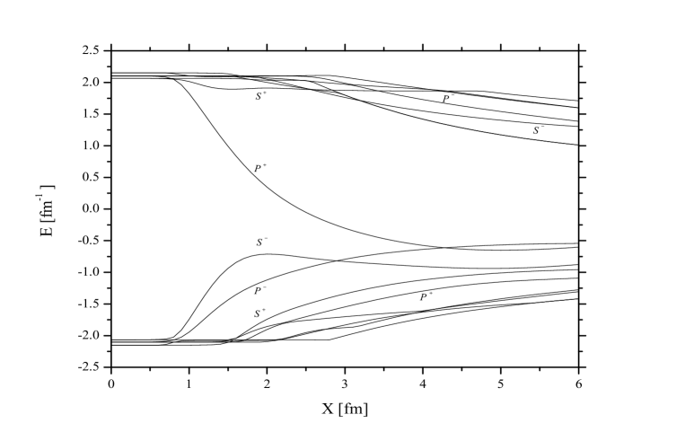
Figure 1: Spectrum of the quark orbits are illustrated as a function of the “soliton size” $X$. Trial profile function is defined by $f(r)=-\pi+\pi r/X$ for $X\leq r$ and $f(r)=0$ for $X>r$. The state coupled with $(K,M)=(0,0)$ is denoted as $S$ and $(K,M)=(1,M)$ as $P_{M}$ ($M=\pm 1,0$) with parity $\pm$. The energy of the three $P$ states are all degenerate.

For $B=3$, it is expected the solution to have a tetrahedral symmetry from the study of the Skyrme model braaten . Therefore, we shall impose the same symmetry on the chiral fields using the rational map ansatz. According to the ansatz, the chiral field can be expressed as manton

$$U(r,z)=\exp\left(if(r)\vec{n}_{R}\!\cdot\!\vec{\tau}\right)$$ (11)

where

$$\vec{n}_{R}=\frac{1}{1+|R(z)|^{2}}\left(\rm{2Re}[\it{R(z)}],\rm{2Im}[\it{R(z)}],\rm{1}-|\it{R(z)}|^{2}\right)$$

and $R(z)$ is a rational map.

Rational maps are maps from $CP(1)$ to $CP(1)$ (equivalently, from $S^{2}$ to $S^{2}$) classified by winding number. It was shown in manton that $B=N$ skyrmions can be well-approximated by rational maps with winding number $N$. The rational map with winding number $N$ possesses $(2N+1)$ complex parameters whose values can be determined by imposing the symmetry of the skyrmion. Thus, $B=3$ rational map with tetrahedral symmetry takes the form;

$$R(z)=\frac{\sqrt{3}iz^{2}-1}{z(z^{2}-\sqrt{3}i)}$$ (12)

where the complex coordinate $z$ on $CP(1)$ is identified with the polar coordinates on $S^{2}$ by $z=\tan(\theta/2){\rm e}^{i\varphi}$ via stereographic projection. Substituting (12) into (11), one obtains the complete form of the chiral fields with tetrahedral symmetry and winding number 3.

Apparently, the chiral fields in (11) takes a spherically symmetric form. Therefore one can apply the numerical technique developed for $B=1$ to find $B=3$ with tetrahedral symmetry wakamatsu .

Demanding that the total energy in (9) be stationary with respect to variation of the profile function $f(r)$,

$$\frac{\delta}{\delta f(r)}E_{total}=0\,\,,$$

yeilds the field equation

$$S(r)\sin f(r)=P(r)\cos f(r)$$ (13)

where

$$S(r)=N_{c}\sum_{\nu}\bigl{(}n_{\nu}\theta(\epsilon_{\nu})+{\rm sign}(\epsilon_{\nu}){\cal N}(\epsilon_{\nu})\bigr{)}\langle\nu|\gamma^{0}\delta(|x|-r)|\nu\rangle$$ (14)

$$P(r)=N_{c}\sum_{\nu}\bigl{(}n_{\nu}\theta(\epsilon_{\nu})+{\rm sign}(\epsilon_{\nu}){\cal N}(\epsilon_{\nu})\bigr{)}\langle\nu|i\gamma^{0}\gamma^{5}\vec{n}_{R}\cdot\vec{\tau}\delta(|x|-r)|\nu\rangle\,\,.$$ (15)

Table 1: A schematic picture of the matrix elements ${\bf A}(K^{\prime}M^{\prime},KM)$ up to $K,K^{\prime}=2$. $S$, $P_{1}$, $P_{0}$ and $P_{-1}$ refer to the elements coupled with $(K,M)=(0,0)$, $(1,1)$, $(1,0)$ and $(1,-1)$ respectively. Other elements are all 0.

	(0 0)	(1 1)	(1 0)	(1 -1)	(2 2)	(2 1)	(2 0)	(2 -1)	(2 -2)
(0 0)	$S$						$S$
(1 1)		$P_{1}$						$P_{1}$
(1 0)			$P_{0}$		$P_{0}$				$P_{0}$
(1 -1)				$P_{-1}$		$P_{-1}$
(2 2)			$P_{0}$		$P_{0}$				$P_{0}$
(2 1)				$P_{-1}$		$P_{-1}$
(2 0)	$S$						$S$
(2 -1)		$P_{1}$						$P_{1}$
(2 -2)			$P_{0}$		$P_{0}$				$P_{0}$

The procedure to obtain the self-consistent solution of Eq.(13) is that $1)$ solve the eigenequation in (7) under an assumed initial profile function $f_{0}(r)$, $2)$ use the resultant eigenfunctions and eigenvalues to calculate $S(r)$ and $P(r)$, $3)$ solve Eq.(13) to obtain a new profile function, $4)$ repeat $1)-3)$ until the self-consistency is attained.

For convenience, we shall take $f_{0}(r)=-\pi{\rm e}^{-r/X}$. To solve Eq.(7), we construct the trial function using the Kahana-Ripka basis kahana ;

$$\Psi^{\pm}=\lim_{K_{max}\rightarrow\infty}\sum_{i=1}^{4}\sum_{K=0}^{K_{max}}\sum_{M=-K}^{K}\alpha_{KM}^{(i)\pm}\varphi_{KM}^{(i)\pm}(r,\theta,\phi)$$ (16)

where $\Psi^{+}$ and $\Psi^{-}$ stand for parity $(-1)^{K}$ and $(-1)^{K+1}$ respectively, $\varphi$ is the Kahana-Ripka basis and $K$ is the grand spin operator which is a good quantum number in the case of $B=1$ hedgehog. The basis is discretized by imposing an appropriate boundary condition for the radial wavefunctions at the radius $r_{max}$ chosen to be sufficiently larger than the soliton size. And also, the basis is made finite by including only those states with the momentum $k$ as $k<k_{max}$. The results should be, however, independent on $r_{max}$ and $k_{max}$.

According to the Rayleigh-Ritz variational method bransden , the upper bound of the spectrum can be obtained from the secular equation for each parity;

$$\rm{det}\left(\bf{A}^{\pm}-\epsilon\bf{B}^{\pm}\right)=0$$ (17)

where

$${\bf A}^{\pm}(K^{\prime}M^{\prime},KM) = \sum_{ij=1}^{4}\int d^{3}x\varphi_{K^{\prime}M^{\prime}}^{(i)\pm}H\varphi_{KM}^{(j)\pm}$$

$${\bf B}^{\pm}(K^{\prime}M^{\prime},KM) = \sum_{ij=1}^{4}\int d^{3}x\varphi_{K^{\prime}M^{\prime}}^{(i)\pm}\varphi_{KM}^{(j)\pm}\,\,.$$

For $K\rightarrow\infty$, the spectrum $\epsilon$ becomes exact. Eq.(17) can be solved numerically.

Since the chiral field in Eq.(11) is less symmetric than the $B=1$ hedgehog, the hamiltonian has no grand spin symmetry. As a result, the states with different grand spin couple strongly and level splittings within the $K$ blocks occur. In Table 1 we present the schematic picture of the matrix elements ${\bf A}(K^{\prime}M^{\prime},KM)$. Although the size of the matrix ${\bf A}(K^{\prime}M^{\prime},KM)$ becomes quite large, due to the symmetry of the chiral fields, the functional space can be rearranged to reduce the size. Consequently, the space is divided with four blocks for each parity.

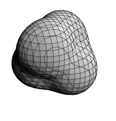
Figure 2: Surface of the baryon-number density with $b_{0}=0.4\,\,{\rm fm^{-3}}$ .

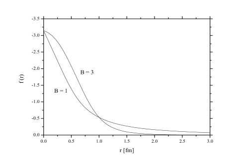
Figure 3: Profile function $f(r)$ of the rational map ansatz for $B=3$, and of the hedgehog ansatz for $B=1$.

Fig. 1 shows the spectrum of the quark orbits as a function of the soliton-size parameter $X$. The $P^{+}$ orbit diving into the negative energy region is triply degenerate. As discussed in kahana , baryon number of the soliton equals to the number of diving levels occupied by $N_{c}$ valence quarks. Thus putting $N_{c}=3$ valence quarks on each of the degenerate levels, one obtains the $B=3$ soliton solution.

Fig. 2 shows the corresponding baryon density. As can be seen, it is tetrahedral in shape. Therefore, we confirm that the lowest lying $B=3$ configuration is tetrahedrally symmetric. This result is consistent with the $B=3$ skyrmion obtained by Braaten et.al braaten .

Fig. 3 shows the self-consistent profile function. For the total energy of the solution we obtain $E_{total}=3596$ MeV which is almost comparable to three times of the $B=1$ mass, and root mean square radius is $\sqrt{\langle r^{2}\rangle}\sim 0.6$ fm. Our soliton seems to be tight object. This is mainly due to the missing of higher components of $K$ in our calculation. Their contribution becomes significant near the surface of the soliton and hence inclusion of the higher components will improve the size of the soliton.

Finally, we would like to mention that our result verifies the validity of the rational map ansatz for the Chiral Quark Soliton Model. The numerical technique used here is quite general and its application to $B\geq 4$ will be straightforward.

Acknowledgements

We are grateful to N.S.Manton for encouraging us to work on this subject and useful comments. We also thank V.B.Kopeliovich for suggesting this topic.

References

• (1) D. I. Diakonov and V. Yu. Petrov, Nucl. Phys. B306, 457 (1986); hep-ph/9802298.
• (2) R. Alkofer, H. Reinhardt and H. Weigel, Phys. Rept. 265, 139 (1996); Chr. V. Christov, A. Blotz, H.-C.Kim, P. Pobylitsa, T. Watabe, Th. Meissner, E. Ruiz Arriola, K. Goeke, Prog. Part. Nucl. Phys. 37, 91 (1996).
• (3) A. Manohar, Nucl. Phys. B248, 19 (1984).
• (4) S. Kahana and G. Ripka, Nucl. Phys. A429, 462 (1984).
• (5) Th. Meissner, E. Ruiz Arriola, F. GrΓΌmmer and K. Goeke Phys. Lett. B227, 296 (1989).
• (6) H. Reinhardt and R. WΓΌnsch, Phys. Lett. B215, 577 (1988).
• (7) M. Wakamatsu and H. Yoshiki, Nucl. Phys. A524, 561 (1991).
• (8) N. Sawado and S. Oryu, Phys. Rev. C58, R3046 (1998); N. Sawado, Phys. Rev. C61, 65206 (2000).
• (9) Th. Meissner, E. Ruiz Arriola, F. GrΓΌmmer, H. Mavromatis and K. Goeke, Phys. Lett. B214, 312 (1988).
• (10) E. Braaten, S. Townsend and L. Carson, Phys. Lett. B235, 147 (1990).
• (11) C. J. Houghton, N. S. Manton and P. M. Sutcliffe, Nucl. Phys. B510, 507 (1998).
• (12) B. H. Bransden and C. J. Joachain, Introduction to Quantum Mechanics (Longman Scientific Technical, 1989)