If sterile neutrinos exist, how can one determine the total solar neutrino fluxes?
Abstract
The 8B solar neutrino flux inferred from a global analysis of solar neutrino experiments is within % () of the predicted standard solar model value if only active neutrinos exist, but could be as large as times the standard prediction if sterile neutrinos exist. We show that the total 8B neutrino flux (active plus sterile neutrinos) can be determined experimentally to about % () by combining charged current measurements made with the KamLAND reactor experiment and with the SNO CC solar neutrino experiment, provided the LMA neutrino oscillation solution is correct and the simulated performance of KamLAND is valid. Including also SNO NC data, the sterile component of the 8B neutrino flux can be measured by this method to an accuracy of about % () of the standard solar model flux. Combining Super-Kamiokande and KamLAND measurements and assuming the oscillations occur only among active neutrinos, the 8B neutrino flux can be measured to % (); the total flux can be measured to an accuracy of about %. The total 7Be solar neutrino flux can be determined to an accuracy of about % () by combining measurements made with the KamLAND, SNO, and gallium neutrino experiments. One can determine the total 7Be neutrino flux to a accuracy of about % or better by comparing data from the KamLAND experiment and the BOREXINO solar neutrino experiment provided both detectors work as expected. The neutrino flux can be determined to about % using data from the gallium, KamLAND, BOREXINO, and SNO experiments.
I Introduction
We describe in this paper analysis procedures that can answer two of the most important questions of neutrino research. How can one determine the total solar neutrino fluxes (, and ) for comparison with solar model predictions? How can one determine the sterile contribution to the total solar neutrino fluxes? Our answers allow for the possibility of an arbitrary mixture in solar neutrino oscillations of active and sterile neutrinos, but require the correctness of the LMA solution of the solar neutrino problems and careful attention to all the sources of error (theoretical as well as experimental) ***This paper was originally written and posted on the electronic archive (hep-ph) before the announcements of the recent SNO results [1, 2] and the improved SAGE measurement of the gallium rate [3] and also before our paper was submitted for publication. We have included in the analysis reported in this version of the paper, which we are submitting for publication, the recent SNO and SAGE measurements. The ideas with respect to the 7Be and 8B neutrinos are unchanged and the numerical results have not been affected significantly, but the present version is more up-to-date with respect to the input data. We have also added, inspired by the SAGE discussion, a detailed analysis of what one can learn about neutrinos before there is a dedicated experiment to measure just the neutrino flux..
We focus first on determining total fluxes by comparing charged current (CC) observables measured in different experiments; this method yields results as independent as possible of uncertainties due to the presence of sterile neutrinos. We then describe how similar techniques can be applied to determine total solar neutrino fluxes using a CC experiment plus a neutrino-electron scattering experiment [or a neutral current (NC) measurement], which yields results that depend more on the sterile neutrino mix but which can nevertheless be relatively accurate.
The numerical values we estimate for the expected precision with which different quantities can be measured rely upon simulations of the performance of the relevant experiments. Therefore the accuracies that we quote are illustrative; the actual accuracies that are obtainable can only be determined once the experimental uncertainties are known.
A Flavor changes occur
Neutrinos change flavors as they travel to the Earth from the center of the Sun. This flavor change was seen directly by the comparison of the Sudbury Neutrino Observatory (SNO) measurement [4] of the charged current reaction for 8B solar neutrinos with the Super-Kamiokande measurement [5] of the neutrino-electron scattering rate (charged plus neutral current). Even more clearly, flavor change has been demonstrated by comparing the neutral current measurement by SNO with the SNO CC measurement [1]. The conclusion that flavor changes occur among solar neutrinos, if based solely upon the comparison of the SNO and Super-Kamiokande event rates, is valid statistically at about the confidence level [4, 6, 7, 8, 9]. The neutral current measurement of SNO increases the significance level for flavor changes among solar neutrinos to the confidence level.
The SNO and Super-Kamiokande results demonstrate simply that new physics is required to resolve the long-standing solar neutrino problem [10], i.e., to understand the origin of the discrepancy between the predictions of the standard solar model [11] and the observed solar neutrino event rates [4, 5, 12, 13, 14, 15, 16]. If one includes the results of the Chlorine [12], Kamiokande [13], SAGE [14], GALLEX [15], and GNO [16] experiments together with the SNO (CC) and Super-Kamiokande results, then the combined measurements require [9] new physics at and, if the relative temperature scaling of the 7Be and 8B neutrino production reactions is taken into account, at . Helioseismological measurements confirm the predicted sound speeds of the Standard Solar Model to better than % and show that stellar physics cannot account for the discrepancies between standard predictions and the observed solar neutrino rates [17].
B Current knowledge of the 8B solar neutrino flux if only active neutrinos exist
The combination of the charged current (CC) and the charged plus neutral-current measurement with Super-Kamiokande has been used by several groups [4, 6, 7, 8] to determine the flux of active 8B neutrinos independent of the solar model. These model-independent determinations of the active flux exploit the similarity between the response functions in the SNO and Super-Kamiokande detectors [4, 6, 18, 19]. In addition, if one includes all the experimental data in a global oscillation solution in which the 8B flux is a free parameter, one obtains a similar (but slightly smaller) allowed range for the 8B neutrino flux [20, 21, 22]. The measurement of the NC rate by SNO [1] provides an independent determination of the active 8B neutrino flux.
All of the analyses yield the same result: if electron neutrinos oscillate into only active neutrinos, then the total 8B neutrino flux is in excellent agreement with the flux predicted by the Standard Solar Model.
This close agreement of the active 8B neutrino flux with the total flux predicted by the Standard Solar Model (SSM) [11, 22] is, if the flux of sterile neutrinos is small, an important confirmation of the quantitative theory of stellar evolution. We summarize below the current best-estimates and the associated uncertainties for the active 8B neutrino flux, .
The agreement, summarized in Eqs. (1)–(4), between the SSM calculated flux and the measured active flux suggests that the sterile neutrino contribution to the 8B neutrino flux may be small. In this paper, we ignore this tempting suggestion and instead concentrate on developing methods to determine experimentally the total 8B and 7Be neutrino fluxes emitted by the Sun, independent of the active-sterile mixture (for a discussion of earlier investigations of sterile neutrinos see Refs. [24, 25]).
If we want to understand the particle physics implications of solar neutrino research, we must determine if sterile neutrinos are present in the solar neutrino flux . Moreover, the original–and still valid–goal of solar neutrino research was [10] to compare solar model predicted and experimentally measured (total) solar neutrino fluxes.
C What can one do if sterile neutrinos exist?
What is the situation if sterile neutrinos exist? The total flux of 8B neutrinos could in this case be much larger than the standard solar model prediction; a major fraction of the total flux that reaches the Earth could arrive in a form that is not detected in solar neutrino experiments. The existing data disfavor (at CL) oscillation into purely sterile neutrinos. Nevertheless, a large sterile component is allowed [22, 26] if oscillations occur into a combination of active and sterile neutrino states (see Refs. [27, 28] for a description of the formalism adopted here). The flux of sterile neutrinos could in principle be large enough to destroy the apparently excellent agreement between the flux predicted by the SSM and the true flux of 8B neutrinos [which is assumed to be pure active neutrinos in the comparison shown above in Eqs. (1)-(4)].
A measurement of the total 8B solar neutrino flux, including the sterile component (if any), will provide information that is important for astrophysics and for particle physics. The motivation for investigating sterile neutrinos is not dependent upon the LSND [29] results that might suggest the existence of sterile neutrinos. Of course, the LSND results are not supported by other experimental results (cf. Ref. [30]) nor by theoretical predictions that have been precisely confirmed (like the helioseismological verifications of the standard solar model), as is the case for the inference of flavor change based upon the SNO-Super-Kamiokande comparison.
Fortunately, the KamLAND reactor neutrino experiment [31], when combined with the SNO measurement of the CC flux, is capable of providing a precise determination of the total, i.e. the active plus the sterile, 8B neutrino flux. We assume throughout this paper the correctness of the currently favored large mixing angle (LMA) solution to the solar neutrino problem. If the LMA solution is not correct, then all global analyses of the available solar and reactor data indicate that either the mass difference, , or the vacuum mixing angle, , will be too small to produce a measurable effect in the KamLAND experiment (see e.g. Refs. [6, 7, 8, 20, 21, 31, 32]). In this case, KamLAND will be unable to provide the information required to determine the total 8B neutrino flux.
Here is the basic physical idea of the method we propose for measuring the total 8B solar neutrino flux. For the KamLAND [31] experiment, one will know accurately the flux of anti-neutrinos from the reactors that contribute significantly to the measured anti-neutrino events. From measurements of the total event rate and the energy spectrum induced by the surviving , the KamLAND experimentalists can determine with precision [31, 33, 34, 35] the anti-neutrino propagation parameters, and . Both the KamLAND measurement and the CC SNO measurements are disappearance experiments for neutrinos (or anti-neutrinos) of similar energies. For the CC measurement made with SNO, one does not know the total 8B neutrino flux created in the Sun. But, assuming conservation of CPT, one can use the propagation parameters and determined by KamLAND and the measured (by SNO) CC rate to solve for the flux that gives the observed result. Summarizing, for the KamLAND experiment one knows the total flux but not the propagation parameters, which are measured. For the SNO CC experiment, one will know (from KamLAND) the propagation parameters and therefore can measure the total flux‡‡‡The method described here is of course more general than the specific application to the KamLAND and SNO experiments. In order to determine the total flux, it is sufficient that one measure a set of observables that do not depend upon the solar neutrino flux (in this paper, the measured quantities in the KamLAND experiment) and a quantity that does depend upon the solar neutrino flux (here, the CC rate in SNO)..

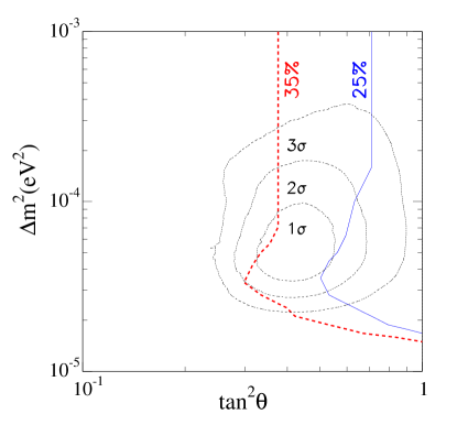
Figure 1 shows the results of a refined global solution for the solar neutrino oscillation parameters that was made (see Sec. II and the Appendix) using all the available solar and reactor data. The figure displays the allowed solar neutrino oscillation contours at , , and . The results are obtained by the procedures described most recently in Ref. [22], where we have used in the present paper the analysis strategy (a) (of Ref. [36]) including the 1496 day Super-Kamiokande data sample [37] as well as the SNO CC, NC and day-night observations [1, 2]. We have also made some improvements (see the Appendix) in the treatment of the uncertainties in the neutrino cross sections and in the correlation of errors.
For comparison, we also show in Fig. 1 the small size of the expected allowed region for KamLAND if this reactor anti-neutrino experiment observes a signal corresponding to the current best-fit point of the solar neutrino analysis. In calculating the KamLAND allowed region, we have made a conservative estimate (see Sec. III C), following the principles discussed in Refs. [38, 39]. Figure 1 shows clearly that KamLAND has the potential for making a precise measurement of the solar neutrino oscillation parameters, provided that the LMA is the correct oscillation solution.
The only complication involved in determining the total 8B flux from a comparison of the KamLAND and SNO CC measurements results from the fact that for the favored Large Mixing Angle (LMA) solar neutrino oscillation solution matter effects in the Sun and the Earth can be significant. Matter effects are unimportant for the KamLAND reactor experiment. The role of matter effects in solar neutrino experiments depends somewhat upon the a priori unknown active-sterile mixture, which introduces a calculable uncertainty in the inferred total 8B neutrino flux.
In summary, the combination of the SNO CC neutrino measurement and the KamLAND anti-neutrino measurement will determine the total (active plus sterile) flux, , of 8B solar neutrinos. By subtracting the previously determined flux (see above), , from , one can determine the flux of sterile solar neutrinos.
Using similar reasoning, we shall also show that the combined Super-Kamiokande and KamLAND measurements can be analyzed to yield an accurate value for the total 8B flux, although in this case the results are somewhat more sensitive to the active-sterile admixture.
D 7Be solar neutrinos
The flux of 7Be solar neutrinos, which in the SSM is predicted[11] to be , can be determined in a model independent way from a global analysis of the solar neutrino data assuming only active neutrino oscillations. For example, the latest analysis by Garzelli and Giunti [7] yields at 99% CL.
We shall also show in this paper that one can extract the value of the 7Be neutrino flux from measurements of the gallium solar neutrino experiments, GALLEX, SAGE, and GNO and the results of the SNO and KamLAND measurements. The value of the 7Be flux that will be derived in this way is relatively insensitive to the assumed neutrino oscillation parameters, although it does depend somewhat on the assumed contributions of the CNO, , and neutrino fluxes which we adopt from the standard solar model. The constraint provided by the Chlorine experiment is not very useful for determining the total 7Be neutrino flux.
One can obtain an independent measurement of the total 7Be solar neutrino flux by comparing data from the KamLAND experiment with data from the BOREXINO [40] solar neutrino experiment. If both the KamLAND and the BOREXINO detectors work as expected, then this method will be more accurate than the methods involving the gallium and chlorine radiochemical detectors.
E Appendix: just for aficionados
The determination of the total solar neutrino fluxes, and even more so the determination of the sterile components of these neutrino fluxes, requires precision in both the experimental measurements and the theoretical calculations and analyses. We present in the Appendix a refined discussion of the theoretical errors, and their correlations, for the absorption cross for the gallium and Chlorine solar neutrino experiments.
F Outline and suggested reading strategy
The outline of this paper is as follows. In Sec. II, we describe the current experimental knowledge of the 8B solar neutrino flux. Our results are summarized in Table I both for the special case of oscillations between purely active neutrinos and for the general case of oscillations between electron neutrinos and an active-sterile neutrino admixture. We limit our analysis to the allowed LMA region of solar neutrino oscillations. We show in Sec. III how one can use the CC measurements with SNO and KamLAND to determine an accurate total 8B solar neutrino flux including experimental and theoretical uncertainties and the possibility of an appreciable active-sterile admixture. We switch to the 7Be flux in Sec. IV and evaluate how well one can determine the total 7Be solar neutrino flux by also using the results of the gallium (GALLEX, SAGE, and GNO) solar neutrino experiments or the Chlorine experiment. In Sec. V, we investigate how well the total 8B and 7Be neutrino fluxes can be determined using the combined measurements of KamLAND and scattering observed in the Super-Kamiokande (Sec. V A) and BOREXINO (Sec. V B) detectors. We show that even in the presence of active-sterile admixtures the total 7Be solar neutrino flux may be measured with relatively high accuracy by comparing results from the KamLAND and the BOREXINO experiments. We describe and analyze in Sec. VI three strategies for determining the total solar neutrino flux in the absence of a dedicated experiment that measures separately the neutrinos. We summarize and discuss our principal conclusions in Sec. VII.
We urge the reader to turn first to Sec. VII and read there the summary and discussion of our main results and their implications. The rest of the paper can then be understood more easily.
II Present knowledge of the 8B neutrino flux
We generalize in this section the determination of the 8B neutrino flux to the case in which oscillates into a state that is a linear combination of active () and sterile () neutrino states,
| (5) |
where is the parameter that describes the active-sterile admixture. This admixture arises naturally in the framework of 4- mixing [28]. The total 8B neutrino flux can be written
| (6) |
where . Clearly, the larger the sterile component, the larger the value of that is inferred from the experimental data.
We have performed a global analysis of the solar neutrino data treating the total 8B neutrino flux as a free parameter. The details of the analysis procedure are the same as those used in Ref. [22] except where we explicitly state otherwise. We concentrate here on the LMA region, , .
To take account of the possibility of oscillations into sterile neutrinos, we determine the allowed regions in the parameter space defined by , , and a third parameter, , that is defined by Eq. (5). It is convenient to introduce the dimensionless parameter,
| (7) |
where is the total 8B neutrino flux in units of the predicted standard solar model flux.
| CL | (active + sterile) | (active) |
|---|---|---|
| 0.99–1.25 | 0.99–1.15 | |
| 0.92–1.47 | 0.92–1.22 | |
| 0.84–1.67 | 0.84–1.29 |
The allowed range of in the three dimensional space of neutrino parameters, , , and , is determined by the equation
| (8) |
Here is the change in that corresponds to a specified confidence limit (CL) for one degree of freedom. The computed values of are minimized for each value of with respect to , , and .
Table I shows the currently allowed range for for both the more general case where a mixture of active and sterile neutrinos is assumed and for the more conventional case in which only active neutrinos are considered. For purely active neutrinos, the range is
| (9) |
and for an arbitrary mixture of active and sterile neutrinos, the range is
| (10) |
The result shown earlier in Eq. (4) for purely active neutrinos is taken from Table I.
How does the possible existence of sterile neutrinos affect the allowed range of 8B neutrino fluxes? We can calculate the dependence of the allowed range of upon with the aid of the inequality
| (11) |
Here is the change in for a specified CL that corresponds to two degrees of freedom ; the computed values of are minimized at each point with respect to , and .
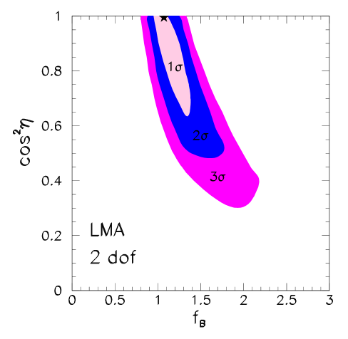
Figure 2 shows the range of as a function of the active-sterile admixture, , that is obtained from Eq. (11) for the , and allowed regions. The allowed regions are defined respect to the global minimum, which corresponds to purely active oscillations with , , and .
Although pure sterile oscillations are forbidden at the 3 CL (cf. Fig. 2), a large sterile admixture in the solar oscillations is still allowed. In fact, with the currently available data, the largest allowed value at of the sterile 8B neutrino flux corresponds to and (for d.o.f.). For this extreme case, we find
| (12) |
The quantity that appears in Eq. (12) is defined, analogous to in Eq. (7), by the relation . The maximum value of is as large as the sum of the active 8B neutrino fluxes (, where , see Ref. [4]) for this special case §§§For 2 d.o.f, the maximum allowed value of is at , but is for d.o.f, see Table I. We have given in the Abstract the maximum value for d.o.f..
What is the maximum allowed sterile contamination of the 8B solar neutrino flux? Minimizing for the global solution with respect to , , and , we find that the allowed range of satisfies
| (13) |
at .
III How can we determine the total 8B neutrino flux using CC reactions?
In this section, we will show how one can determine the allowed range of the total 8B neutrino flux using the results of the KamLAND reactor neutrino experiment and the SNO CC solar neutrino experiment. We shall also estimate the accuracy with which one can determine the total 8B flux.
Since we consider here only CC reactions that result from disappearance experiments, the only difference between the role of active neutrinos and and sterile neutrinos arises from matter effects in the Earth and in the Sun. Since sterile neutrinos do not interact with matter, the effective potential for the – evolution in matter is , since . The effective potential is approximately half the potential for –, , where is the potential for the active neutrinos and . (The difference is exactly half for a medium with equal number of neutrons, protons and electrons because with .) We shall evaluate the expected dependence of the inferred total 8B flux on the admixture of sterile neutrinos [cf. Eq. (5)].
In Sec. III A we present the formulae that are used to determine the 8B flux with the aid of the KamLAND and SNO CC experiments and in Sec. III B we illustrate the effect on the inferred 8B flux of the maximum allowed (at ) sterile admixture. We estimate in Sec. III C the precision with which the 8B flux can be determined including all the principal known sources of uncertainties.
The reader who is interested in how well we can determine the 8B flux, but does not need to know the details of the procedure, can get the main results by glancing at Fig. 2 and Fig. 3 and Table II.
In Sec. V A, we investigate how well the total 8B flux can be determined using KamLAND in combination with the scattering experiment, Super-Kamiokande.
A Relations that determine the total flux
Suppose KamLAND observes a signal that corresponds to LMA oscillations with parameters . We assume the validity of the CPT theorem so that constraints on anti-neutrino oscillation parameters obtained from the KamLAND experiment apply to solar neutrino experiments. We can then extract the 8B neutrino flux from the following relation:
| (14) |
where
| (15) |
is the CC rate for the SNO experiment[4] that is predicted[11, 22] by the standard solar model in the absence of oscillations and is the average survival probability for electron-flavor neutrinos created in the Sun. Also, is the neutrino energy and is the weighted average -d interaction cross-section, including the experimental energy resolution function, , where is the measured (true) recoil kinetic energy of the electron. Thus
| (16) |
The lower limit, , in the integral in Eq. (16) is taken here to be the threshold used by the SNO Collaboration in Ref. [4] ( MeV). The calculated value for the CC rate is not sensitive to the assumed value of , as long as MeV.
The energy-averaged survival probability, for at SNO can be computed using the propagation parameters, ,observed at KamLAND. Thus
| (17) |
B Illustrative dependence of total flux upon active-sterile admixture
How much does a sterile neutrino admixture affect the inferred total 8B neutrino flux? The dominant dependence on the sterile admixture arises from matter effects within the Sun for larger and within the Earth for smaller .
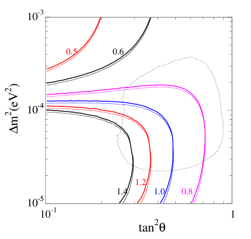
Figure 3 shows the isocontours of in the LMA region for the pure active case (thicker lines) and for the active-sterile case (thinner lines). The isocontours are not very different for the two cases. Moreover, the dependence on Earth matter effects can be avoided experimentally by using only the daytime CC measurement, once sufficient statistics are available. The robustness of the inferred 8B solar neutrino flux can be tested by comparing the 8B flux inferred using only daytime CC measurements with the flux that is inferred when nighttime data (with corrections for Earth matter effects) are added to the daytime data.
In Fig. 3,we also show the LMA contour (the dotted contour) obtained by the global analysis of the solar neutrino data for the purely active case . Within the LMA region, the maximum difference between the value of inferred allowing for possible sterile neutrinos and the value obtained assuming only active neutrino oscillations is % and %. The dependence upon the active-sterile mixture could become negligible if the correct lies in the lower part of the LMA region and only daytime data is used from the SNO CC measurements.
We conclude from Fig. 3 that existence of sterile neutrinos will not prevent an accurate measurement of the total 8B neutrino flux.
C How accurately can the total 8B flux be determined?
What is the overall precision expected in the determination of the total 8B flux? From Eq. (14) we can derive the anticipated precision as
| (18) | |||||
| (19) |
where the errors are combined quadratically.
The current value of the first term in Eq. (19), the uncertainty (statistical and systematic) of the measured CC rate in SNO, is [1] %. This uncertainty will undoubtedly decrease as the results of analyzing more SNO CC data are reported.
The second term in Eq. (19) represents the uncertainty in the -2H absorption cross section. Much progress has been made recently in evaluating this cross section, see e.g. Refs. [41, 42], which has led to an estimate % for the cross section uncertainties other than radiative corrections. No definitive calculation has yet been made of the radiative correction for the CC reaction, but a reasonable estimate [41] is that the cross sections given in Ref. [41] might be increased by %. We adopt here a conservative uncertainty of % ; the precise value chosen for is not very important at this stage since other uncertainties are dominant. The neutrino flux contribution to is negligible for our purposes [4, 5, 11]
A detailed simulation is required to estimate , i.e., the uncertainty in the average electron neutrino survival probability for 8B solar neutrinos observed in the SNO CC experiment as will be determined by future KamLAND measurements. Here is how we estimate this uncertainty. We generate the expected KamLAND signal for a fine grid of points, that spans the space of the allowed oscillation parameters determined from solar neutrino experiments. For each grid point, we obtain the allowed region by a analysis. We use statistical errors corresponding to three years of data taking at KamLAND, observing anti-neutrinos from reactors working at a constant % of the maximal power. To be conservative, we also assumed a neutrino energy threshold of MeV, in order to ensure that the effects of natural radioactivity would be small. More details on the KamLAND experiment can be found in Ref. [31]; details regarding the neutrino cross sections, statistical procedures, and reactor fluxes used in the present paper are described in Refs. [38, 39].
| % | % | |||
|---|---|---|---|---|
| 1.09 | ||||
| 0.98 | ||||
| 1.51 | ||||
| 1.02 | ||||
| 0.94 | ||||
| 1.30 | ||||
| 1.01 | ||||
| 0.98 | ||||
| 1.57 |
In computing the inferred values of , we take account of the fact that there could be a significant component of sterile neutrinos in the incident 8B solar neutrino flux. We therefore consider all active-sterile admixtures permitted by the global oscillation solution shown in Fig. 1. The numerical constraint on the currently allowed admixture is given in Eq. (13).
In principle, for each simulated point there are two allowed KamLAND regions, one around and and another around and . We discuss here only the range of parameters within the first octant for the mixing angle since global solar neutrino solutions show [6, 7, 8, 20, 21, 22, 32] that the first octant is preferred. For each simulated KamLAND allowed region centered on a specific , we compute . We repeated this procedure for a grid of points in the range , . The estimated uncertainty in varies with the grid point .
Table II presents the best-fit value of , the uncertainty in , and the total expected uncertainty in inferring from the combined SNO CC and the KamLAND neutrino reactor measurements for a representative set of possible results for and . In all the cases shown in Table II, we have used % and % (see previous discussion). The uncertainty contributed by the possibility that sterile neutrinos exist, i.e., , is rather modest; is typically reduced by % from the value shown in Table II.
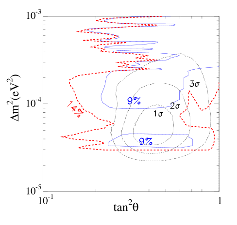
Figure 4 shows the % and the % contours for the maximum percentage deviation from the best-fit value. To provide a context, the figure also displays the , and allowed LMA regions obtained by a global fit to the available solar and reactor data. Within almost all of the current 1 LMA allowed region, the comparison of the KamLAND and the SNO CC data will determine the total 8B flux with an uncertainty that is less than %; the uncertainty can be less than % over a significant fraction of the current allowed domain. About 6% of the current estimated uncertainty is due to the experimental error in the SNO CC measurement, which hopefully will be reduced as more CC data are accumulated.
For some purposes, it is convenient to know what is the average expected accuracy in the determination of . We have computed this average with the aid of a Monte Carlo sampling of the currently allowed solar neutrino oscillation parameters shown in Fig. 1. The average positive and negative uncertainties are approximately equal (cf. Table II). We find an average uncertainty of
| (20) |
A very significant component of comes from . We find, averaged over the current solar neutrino oscillation region,
| (21) |
The sterile neutrino contribution to the 8B neutrino flux can be determined by subtracting the active neutrino flux from the total neutrino flux. Thus,
| (22) |
Using, as described above, the errors for the total and the active fluxes of % and % (assumed for the SNO NC measurement), respectively, we estimate that the sterile component of the 8B neutrino flux can be determined to a precision of about %.
IV How well can we determine the total 7Be flux using CC (radiochemical) experiments?
We show in this section how the total 7Be solar neutrino flux can be determined, with the judicial aid of other neutrino fluxes predicted by the standard solar model [11], by combining the results of the GALLEX [15],GNO [16], and SAGE [14] gallium solar neutrino experiments with the KamLAND and SNO CC measurements. We shall also explore the extent to which the Chlorine experiment [12, 43] can provide independent information about the 7Be solar neutrino flux.
We limit ourselves in this section to detectors that only observe or , specifically, we consider here only the radiochemical gallium and chlorine experiments and the reactor anti-neutrino experiment, KamLAND. This limitation simplifies the calculations with respect to the role of the sterile neutrinos. However, the radiochemical experiments suffer from the disadvantage of a lack of energy discrimination, which introduces uncertainties involving the roles of the , , and CNO neutrinos.
| Source | Flux | Ga (SSM) | Ga (LMA) |
| (SNU) | (SNU) | ||
| 69.7 | 40.4 | ||
| 2.8 | 1.51 | ||
| 0.1 | 0.023 | ||
| 34.2 | 18.6 | ||
| 12.2 | 4.35 | ||
| 3.4 | 1.79 | ||
| 5.5 | 2.83 | ||
| 0.1 | 0.03 | ||
| Total |
We begin by describing in Sec. IV A the general procedure for determining the 7Be neutrino flux. We then evaluate in Sec. IV B the principal sources of error, taking account of experimental and theoretical uncertainties as well as the possibility of an appreciable sterile neutrino component in the incident solar neutrino flux. We present in Sec. IV C the numerical results for the uncertainties due to different factors and evaluate the overall accuracy with which the total 7Be flux can be determined.
Using data from either the gallium or the Chlorine [12] experiments, the same procedure can be applied for inferring the 7Be neutrino flux. For simplicity, we describe the procedure in Sec. IV A–Sec. IV C with reference to the more promising case provided by the gallium experiments. In Sec. IV D, we investigate how accurately one can determine the 7Be flux using data from the Chlorine experiment instead of the gallium experiment.
In Sec. V B, we use the techniques developed in this section to explore the accuracy with which KamLAND and BOREXINO can determine .
A Procedure for determining the total 7Be solar neutrino flux
.
Table III shows the neutrino fluxes and the event rates in the gallium solar neutrino experiments that are predicted by the standard solar model [11, 22] . The table also shows the event rate predicted by the best-fit LMA solution. From Table III it is clear that one must make a strong assumption about the neutrino flux in order to determine the 7Be flux. One must also make assumptions regarding the best-value and the uncertainties in the CNO and fluxes. This situation is different than the purely empirical procedure described in Sec. III for determining the 8B neutrino flux; the 8B solar neutrino flux can be determined independent of all considerations regarding the standard solar model.
We assume throughout this section the correctness of the calculated standard solar model [11] values for the neutrino fluxes and their uncertainties, except for the 7Be and 8B fluxes which we want to determine from solar neutrino experiments¶¶¶The ultimate astronomical goal of solar neutrino experiments is to determine all of the solar neutrino fluxes directly from experiment, but there are too few experimental constraints to make this possible at the present time..
Fortunately, as we shall see, if we assume the SSM predictions and their uncertainties for all but the 7Be and 8B fluxes, then we can infer an interesting range for the total solar 7Be neutrino flux if we use data from the gallium experiments. The situation is less promising if we use data from the Chlorine experiment rather than the gallium experiments.
Suppose that KamLAND observes a signal that corresponds to oscillations with parameters , then the expected event rate in the gallium experiments is a sum of the contributions from the different neutrino fluxes, namely,
| (24) | |||||
In the last term in Eq. (24), we include the contributions from , , CNO and neutrinos. By analogy with Eq. (7), we have defined the factors as the ratios between the “true” solar neutrino fluxes and the fluxes predicted by the standard solar model.
We can solve Eq. (24) for the 7Be solar neutrino flux as follows. We substitute into Eq. (24) the value of determined, independent of the solar model, from the KamLAND and SNO CC measurements, as discussed in the previous section (Sec. III). We also assume as a first approximation that all the solar neutrino fluxes but the 8B and 7Be fluxes are equal to the values predicted by the SSM; we investigate later the accuracy of this approximation. With these assumptions, we can then solve for by equating SNU. Thus (26)
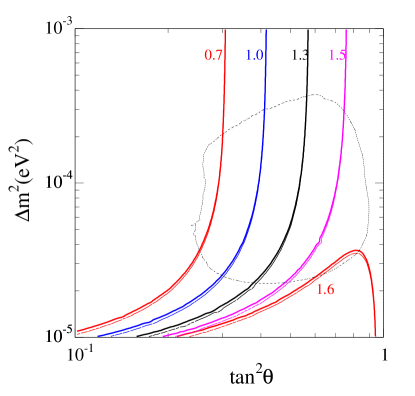
Figure 5 shows that for the 7Be neutrino flux the uncertainty due to the potential effect of sterile neutrinos is small. The figure shows the isocontours of in the LMA region for the case of purely active case (thicker lines) and for the mixture of active and sterile neutrinos with (thinner lines). Within the () parameter region, the difference in the value of between the two oscillation scenarios is less than % (%).
B Principal sources of uncertainty in determining the 7Be total flux
The uncertainty in the inferred total 7Be solar neutrino flux can be estimated from Eq. (26). Including just the largest contributions, we can write the fractional uncertainty in the total 7Be neutrino flux as
| (28) | |||||
where is the uncertainty from the experimental error of the gallium rate, is the theoretical uncertainty from the calculated -Ga absorption cross sections [44], is the uncertainty arising from the allowed range of neutrino parameters determined by KamLAND and SNO [which affects all of the averaged survival probabilities in Eq. (26)], and is the uncertainty due to the quoted errors in the standard solar model calculation of the CNO fluxes (see Table III and Ref. [11]). We have omitted from Eq. (28) a number of sources of error that contribute only relatively small uncertainties. The omitted sources of error [and their range of contributed uncertainties for a representative set of oscillation parameters] include the experimental error in the SNO CC measurements [()%], the uncertainty in the theoretical absorption cross section for the SNO CC experiment [()%], and the uncertainty in standard solar model calculation of the neutrino flux [()%].
We now discuss how we estimate the uncertainties in . Because they require special treatment, we first discuss the uncertainty arising from the theoretical neutrino capture cross sections for gallium and then discuss the uncertainty resulting from the range of allowed neutrino parameters determined by KamLAND∥∥∥The SNO CC results are used to select the first quadrant for (cf. Fig. 1), but for brevity we refer to the range of neutrino parameters determined by KamLAND..
To evaluate the uncertainties arising from the gallium absorption cross sections for neutrino sources with continuous energy distributions, we use Tables 2–4 of Ref. [44]; these tables give the best-estimate and the limits for the theoretical cross sections. For the neutrino lines from 7Be and , we have checked that the shape of the line [45] does not affect significantly the error estimate. Therefore, we use for the 7Be and lines the error estimates given in Eq. (41) and Eq. (42) of Ref. [44]. We have adopted the conservative procedure described in Sec. XII.A.4 of Ref. [44], in which the uncertainties in all of the low energy ( MeV) cross sections are fully correlated, while the uncertainties for the (8B) neutrinos above MeV are treated separately. All of the cross sections for low energy neutrinos move up or down together, reflecting the fact that the dominant uncertainties for low energy neutrinos are common to all sources. For higher-energy neutrinos, a number of excited states dominate the calculated absorption cross section (For a more explicit description of how the cross section errors are treated, see the Appendix.).
To calculate the uncertainty associated with the range of allowed neutrino parameters determined by KamLAND, we first solve Eq. (26) with the appropriate average survival probabilities computed for each neutrino oscillation point () in the allowed region (cf. Fig. 1). We consider active-sterile neutrino admixtures permitted by the currently allowed global oscillation solution [see Eq. (13)]. The solution of Eq. (26) determines for that particular point in oscillation parameter space. Then we construct a allowed region, a set of points , around the chosen point using the simulated characteristics of the KamLAND experiment (see Sec. III C and Refs. [31, 38, 39]). We define for the chosen () to be the maximum (or minimum) value of . In practice, the inclusion of sterile neutrinos only slightly affects the computed range of .
For all other quantities, we estimate the associated uncertainty at a particular point () in the following way. Given a source of uncertainty (for example, the measured capture rate for the gallium experiments) with 1 error , we obtain from the relation
| (29) |
Here we denote by the value of obtained from Eq. (26) when all the parameters are assigned their best-estimate values. The quantity is calculated from Eq. (26) using the best-estimate values of all variables except ; the variable is set equal to its best-fit value the corresponding 1 uncertainty. In calculating , we shift the three CNO neutrino fluxes by simultaneously and in the same direction, reflecting the correlation between the CNO fluxes in the standard solar model.
The uncertainty, , that is calculated from Eq. (29) will in general depend upon the assumed value for () within the KamLAND allowed region. This dependence persists even if is independent of () (which is true, e.g., for the measured gallium capture rate). In fact, the positive and negative values for will generally not be equal.
| Uncertainties (%) | |||||||
|---|---|---|---|---|---|---|---|
| 1.15 | 22 | 4.5 | |||||
| 1.31 | 20 | 4.0 | |||||
| 0.63 | 24 | 8.1 | |||||
| 1.09 | 23 | 4.8 | |||||
| 1.25 | 20 | 4.2 | |||||
| 0.58 | 36 | 9.1 | |||||
| 1.26 | 21 | 4.0 | |||||
| 1.40 | 19 | 3.6 | |||||
| 0.73 | 31 | 6.6 | |||||
C The accuracy with which the total 7Be flux can be determined
Table IV presents the calculated uncertainties and the best-fit values of for a representative set of possible neutrino oscillation parameters, (), that may be obtained from the KamLAND measurements . The largest uncertainty, %, is due to the experimental error on the measured gallium rate [14, 15, 16]. The two next largest uncertainties, both %, arise from the theoretical calculation of the gallium absorption cross sections and the simulated errors in the KamLAND measurements. The rather large uncertainty due to the gallium cross sections requires explanation since the uncertainties on the individual cross sections are much smaller [44] [e.g., % for neutrinos and % (average) for 7Be neutrinos]. The amplification in the error due to the cross sections arises because all of the low energy cross section errors are fully correlated. The gallium cross section errors are added linearly in calculating [cf. Eq. (26)] rather than being combined quadratically.
We have also computed a representative (average) error in the determination of the total 7Be flux by a Monte Carlo sampling of the allowed KamLAND oscillation region shown in Fig. 1. We find
| (30) |
Figure 6 shows the contours of the maximum percentage deviation (in absolute value) from the local best-fit value of . The figure shows that within the currently allowed solar neutrino oscillation region the expected uncertainty in the determination of the 7Be flux is of the order of % [in agreement with Eq. (30)].
D Can one use the Chlorine experiment to determine the 7Be solar neutrino flux?
We can derive an expression for in terms of the measured event rate in the Chlorine [12, 43] solar experiment. Replacing “gallium” by “chlorine” everywhere in Sec. IV A–Sec. IV C, we find (32) where SNU [12]. Equation (32) is the analogue for the Chlorine experiment of the previously derived Eq. (26) that was used in the discussion of extracting for the gallium experiments.
Table V lists the best-fit values of that were obtained by solving Eq. (32) for different pairs of oscillation parameters, . The best-fit values of obtained from the the Chlorine experiment are smaller than the best-fit values inferred using the gallium data (cf. Table IV and Table V). Using the chlorine data, one can even get negative (i.e., unphysical) solutions for .
The basic reason for the difficulty in determining is that the large expected rate from the 8B neutrino flux, even after reduction due to neutrino oscillations, can account for all the observed rate in the Chlorine experiment [46]. The contribution from the 7Be neutrinos is obtained by subtracting the large and somewhat uncertain expected contribution from 8B neutrinos (and the contributions from CNO and neutrinos that are expected to be much less important) from the total measure chlorine rate. The result is a rather small and uncertain remainder, which can be attributed to 7Be neutrinos.
Table V also presents the most important sources of uncertainty for inferring the value of using the chlorine, rather than the gallium, data. Since the inferred best-fit values for that are obtained using the chlorine data are very small (or even negative), we show in Table V the associated shifts in the prediction of . For the much more reliable inferences from gallium data, we show instead in Table IV the percentage shifts, not the actual numerical shifts.
| Uncertainties | ||||||||
|---|---|---|---|---|---|---|---|---|
| 0.17 | ||||||||
| 0.20 | ||||||||
| 0.07 | ||||||||
| 0.12 | ||||||||
| 0.16 | ||||||||
| 0.25 | ||||||||
| 0.26 | ||||||||
| 0.16 | ||||||||
The largest uncertainties in determining using the chlorine data are caused by the experimental errors in the chlorine absorption rate () and the SNO CC absorption rate (). The uncertainty in the chlorine neutrino absorption cross sections are also significant ( to , depending upon the neutrino oscillation parameters). To be explicit, the uncertainties in due to the theoretical uncertainties in calculating the chlorine neutrino absorption cross sections that were used in constructing Table V were evaluated from the following equation,
| (33) |
(See the Appendix for more details regarding the treatment of the cross section errors.) Even the CNO fluxes () and the SNO CC absorption cross section () contribute non-negligible errors. The uncertainty from sterile neutrinos is small () and does not significantly affect the total uncertainty.
Remarkably, the individual uncertainties in which arise from several different sources are larger than the current best-fit values of (see Table V).
For the chlorine based determination, we have computed a representative (average) shift in by a Monte Carlo sampling of the allowed KamLAND oscillation region shown in Fig. 1. We find
| (34) |
This uncertainty is so large as to render not very useful the determination of with the aid of chlorine data.
V How well can KamLAND plus scattering experiments determine the total 8B and 7Be fluxes?
In this section, we show how data from KamLAND can be combined with scattering data obtained with the Super-Kamiokande and BOREXINO experiments in order to determine, respectively, the total 8B (Sec. V A) and 7Be (Sec. V B) solar neutrino fluxes. As discussed before, the advantage of using purely CC measurements to determine the fluxes is that the answers depend only mildly on the active-sterile admixture. On the other hand, scattering measurements have the advantage of smaller uncertainties in the interaction cross sections. Moreover, for the determination of the 7Be flux, BOREXINO depends less strongly on other neutrino fluxes predicted by the standard solar model than do the radiochemical experiments, Chlorine, GALLEX, SAGE, and GNO.
A How well can KamLAND and Super–Kamiokande determine the total 8B flux?
In this section, we show how data from the Super-Kamiokande and KamLAND experiments can be combined to measure the total 8B neutrino flux. We shall see that the determination using Super-Kamiokande and KamLAND yields, on average, a value for the total flux than is comparable in precision to what is expected to be obtained using SNO and KamLAND. The systematic uncertainties are different in the two experiments, SNO and Super-Kamiokande. Therefore, it will be important to compare the total 8B neutrino flux that is inferred using Super-Kamiokande and KamLAND with the value that is obtained using SNO and KamLAND. If the uncertainties are correctly estimated, then the two methods should agree within their quoted errors.
The advantage of using purely charged current measurements with SNO and KamLAND to determine the total 8B flux is that the answer depends only very slightly upon the unknown active-sterile mixture (as discussed in Sec. III). The principal advantages of the Super-Kamiokande experiment in the present context is that the neutrino interaction cross section is accurately known [47] and the statistical and systematic errors have already been extensively investigated [5]. However, as we shall see below, when using Super-Kamiokande there is a significant uncertainty (% and %) in the total 8B flux due to the active-sterile mixture, at least with our present knowledge of .
The average survival probability for 8B solar neutrinos can be written in the form
| (36) | |||||
where is the probability of oscillating into active neutrinos and is the ratio of the the and elastic scattering cross-sections. The expected sensitivity of to the principal sources of errors can be calculated from the following equation:
| (37) |
We suppose that KamLAND will observe (with associated uncertainties that we simulate with a Monte Carlo) the rate predicted for the global best-fit point shown in Fig. 1. For purely active oscillations, we find that
| (38) |
where the first error corresponds to the Super–Kamiokande experimental uncertainty and the second error is caused by the finite size of the allowed KamLAND region in oscillation parameter space. The combined KamLAND and Super-Kamiokande measurement will, for purely active neutrinos, yield a determination for the total 8B flux that is more accurate than can be obtained with the SNO CC measurement and KamLAND. Within the 1 LMA region, the average uncertainty in the combined KamLAND and Super-Kamiokande measurement for the total active 8B neutrino flux is expected to be
| (39) |
For purely active neutrinos, Super-Kamiokande and KamLAND may provide us with a more accurate determination of the total 8B neutrino flux than SNO CC and KamLAND [cf. Eq. (20) and Eq. (39)].
Allowing for the currently allowed (%) sterile admixture, we find for the best fit point
| (40) |
The last error in Eq. (40) corresponds to the present 1 uncertainty from the active-sterile admixture . The average uncertainty in the combined KamLAND and Super-Kamiokande measurement for is expected to be %, within the 1 LMA region and if the sterile admixture is as large as currently allowed.
B How well can KamLAND and BOREXINO determine the total 7Be flux?
In this section, we show how data from the KamLAND and BOREXINO experiments can be combined to measure the total 7Be neutrino flux. The principal advantage of using the BOREXINO experiment for this purpose is that the signal in the BOREXINO experiment [40] is predicted to be dominated by 7Be neutrinos, whereas 7Be solar neutrinos are expected to contribute only a relatively small (and unlabeled) fraction to the observed event rate in the gallium and chlorine radiochemical measurements (see Table III)******The BOREXINO detector can measure the energy of the recoil electrons produced by scattering. The radiochemical detectors do not have energy resolution, only an energy threshold..
However, unlike the cases involving the gallium and chlorine experiments that were discussed in Sec. IV, which include only (CC) absorption, the BOREXINO experiment detects both scattering and and scattering. One must consider in the present case the extent to which the active-sterile neutrino admixture influences the detected event rate for each set of oscillation parameters, , determined by KamLAND. As we shall see quantitatively in the following discussion, this uncertainty regarding the sterile admixture does not decrease significantly the overall accuracy of the inferred total 7Be neutrino flux.
The average survival probability for active neutrinos can be written conveniently in the form
| (42) | |||||
where is the oscillation probability of neutrino fluxes of source into active neutrinos and is the ratio of the the and elastic scattering cross-sections.
The expression for has the same form for the case in which the KamLAND and BOREXINO experiments are considered together as for the previously discussed cases involving the gallium experiments [see Eq. (26)] and the chlorine experiment [see Eq. (32)]. Using the average survival probability defined in Eq. (42), we can write
| (43) | |||
| (44) |
In the last term of Eq. (44), we include the contributions from , and CNO neutrinos. The contribution from 8B neutrinos is negligible because the observed 8B neutrino flux is about a factor of smaller than the predicted SSM 7Be neutrino flux and because 8B neutrinos primarily produce high energy recoils electrons that the BOREXINO detector can distinguish from the low energy recoil electrons produced by 7Be neutrinos.
The expected sensitivity of to different sources of errors is given by
| (45) |
In order to estimate the accuracy of this method for determining , we suppose that KamLAND will observe (with associated uncertainties that we simulate with a Monte Carlo) the rate predicted for the global best-fit point††††††The predicted rate in units of the expected SSM rate is , see Ref. [36]. shown in Fig. 1 and that BOREXINO also will observe a signal corresponding to this best-fit point (with associated uncertainties). In the absence of any published data, we estimate that-based upon experience in previous solar neutrino experiments [4, 5, 12, 14, 15, 16]-that BOREXINO will achieve a systematic uncertainty of between % and % . We estimate in this way that the combined experiments will yield a determination of that is, for purely active oscillations,
| (46) |
where the first error corresponds to the BOREXINO experimental uncertainty, the second to the uncertainty in the reconstructed KamLAND region, and the last error is due to the theoretical uncertainty in the predicted CNO fluxes. Within the 1 LMA region, the average uncertainty in the combined KamLAND and BOREXINO measurement for the total active 7Be neutrino flux is expected to be
| (47) |
If we allow for a 25% sterile admixture, we find
| (48) |
The last error in Eq. (48) corresponds to the present 1 uncertainty from the active-sterile admixture . The numbers in parentheses in Eq. (46) and Eq. (48) correspond to assuming the larger systematic uncertainty, %, for the BOREXINO measured rate.
For , the average uncertainty in the combined KamLAND and BOREXINO measurement is expected to be %, within the 1 LMA region and if the sterile admixture is as large as currently allowed,
VI Determination of the neutrino flux
In this section, we analyze three strategies for determining the total solar neutrino flux without requiring a dedicated experiment that measures only the neutrinos. We first describe in Sec. VI A how one can make a crude determination of the neutrino flux using the measured Gallium, Chlorine, and SNO (CC) event rates [3, 12, 15, 16] and the standard solar model predictions for all but the 8B, 7Be, and solar neutrino fluxes. This part of the discussion is similar to the analysis described in Ref. [3], although we evaluate explicitly the uncertainty caused by the finite size of the allowed region in oscillation parameter space . We then determine in Sec. VI B how well one can infer the flux using just the Gallium and the SNO measurements and the BP00 predictions for the other neutrino fluxes, especially the 7Be neutrino flux. The unknown sterile-active mixture contributes only a negligible error using the strategies described in Sec. VI A and Sec. VI B. Next, we show in Sec. VI C how the precision of the determination of the flux can be improved by using, in the future, the results from KamLAND (to constrain the neutrino oscillation parameters) and from BOREXINO (to constrain the 7Be neutrino flux). The principle of this strategy has also been discussed by the SAGE collaboration [3].
The theoretical error on the neutrino flux is % (see Ref. [11]), which is an order of magnitude smaller than the estimated errors that we find in this section on the empirically derived values of . To achieve a precision of % or better in the determination of the solar neutrino flux will require a dedicated and accurate experiment devoted to measuring the flux.
Throughout this section, we treat the flux and the flux as a single variable because they are so closely linked physically [48]. The two reactions are linked because the reaction is obtained from the reaction by exchanging a positron in the final state with an electron in the initial state. Thus the rates for the two reactions are proportional to each other to high accuracy [49]. For convenience, we denote the sum of the and fluxes as simply .
A Using Chlorine, Gallium, and SNO data and BP00 predictions
In this subsection, we show how data from the chlorine, gallium, and SNO experiments can be combined with the BP00 predictions for the CNO and fluxes to determine the total neutrino flux.
The reduced solar neutrino flux, defined (by analogy with ) with respect to the predicted standard solar model sum of the and fluxes, can be written as:
| (50) | |||||
Here the sum over in Eq. (50) refers to the three CNO neutrino sources and the neutrinos (see Table III).
We insert in Eq. (50) the expression for in terms of the Chlorine and SNO rates and the standard solar model CNO and neutrino fluxes. Explicitly,
| (52) | |||||
For the special case of the best fit point in the LMA solution region, we find
| (53) |
The first error in Eq. (53), (), results from the weighted average experimental error for the Gallium experiment [3, 15, 16]. The second error, (), reflects the uncertainties in the calculated neutrino absorption cross sections on gallium [44]. The third error, (), is caused by the uncertainties in the calculated standard solar model CNO fluxes [11]. The fourth error, (), derives from the measurement errors in the SNO CC experimental data [1] and neutrino absorption cross section [41]. The fifth error, (), results from the experimental error for the Chlorine event rate [12] and the sixth error, (), reflects the uncertainties in the calculated neutrino absorption cross sections for Chlorine [48, 50]. The physical constraint, , was imposed in obtaining these errors.
Within the LMA allowed region, we find that the central value of can vary in the range and the best-fit value can be determined with an average uncertainty of %. The range of central values of always exceeds the BP00 value because the observed Chlorine rate implies a low value of . Since the largest contributions to the Gallium rate are from neutrino and 7Be neutrinos, a low 7Be flux implies a relatively high flux.
We can summarize as follows the results of the simulations carried out within the allowed LMA region for the flux:
| (54) |
The first error in Eq. (54) results from the allowed range of neutrino oscillation parameters and the second error results from the uncertainties in all other recognized sources of errors, combined quadratically. The result given in Eq. (54) should be compared with the quoted estimate by the SAGE collaboration [3], . This agreement is very welcome since the SAGE paper points out that they made “Several approximations…whose nature cannot be easily quantified.”
B Using Gallium and SNO data and BP00 predictions
In this subsection, we determine the range of allowed values for using the BP00 predictions (and uncertainties) for the 7Be neutrinos as well as the CNO and neutrinos. We use in this subsection data only from the Gallium and SNO solar neutrino experiments.
Following the same line of reasoning as in section VI A, we find for the best fit point in the LMA allowed oscillation region,
| (55) |
Just as in Eq. (53), the first error in Eq. (55), (), is the experimental error from the weighted average event rate in the gallium experiments, the second error,(), is due to the neutrino absorption cross section on gallium, the third error, (), is due to the uncertainties in the BP00 predictions of the CNO neutrino fluxes, the fourth error, (), contains the uncertainty in the SNO CC experimental rate and the calculated absorption cross sections on deuterium. The uncertainty in the BP00 prediction for the 7Be neutrino flux contributes the last error, (), in Eq. (55).
Within the allowed LMA region, we find the central value of varies in the range ; the best-fit value of can be determined with an average uncertainty of %. We can summarize the determination of as follows:
| (56) |
where the first error is the uncertainty due to the neutrino oscillation parameters and the second error contains the uncertainties from all other sources.
C Using BOREXINO, KamLAND, Gallium and SNO data and BP00 predictions
In this subsection, we show how the uncertainty in could be improved by using the KamLAND data to determine the neutrino oscillation parameters and the BOREXINO data, together with the KamLAND oscillation parameters, to constrain . We start with Eq. (50) but now use as determined from BOREXINO and KamLAND data [Eq. (44)].
We find that for the best-fit LMA solution (assuming that BOREXINO finds the rate expected for this best fit point),
| (57) |
The first error shown in Eq. (57), (), is the experimental error on the measured Gallium event rate, the second error, (), represents the uncertainties from the calculated gallium cross sections. The third error, , is from the predicted CNO fluxes and the fourth error, (), contains the uncertainties from the SNO experimental data and calculated deuterium absorption cross sections. The range of oscillation parameters within the KamLAND reconstructed region gives the fifth error, (), and the sixth error, ( []), results from the uncertainty in the measured BOREXINO event rate [which we take to be 5% (10%)]. The unknown active-sterile admixture (which goes in the direction of lowering ) contributes the last error shown in Eq. (57).
On average, the the precision expected using the Gallium, KamLAND, and SNO experiments is
| (58) |
The dominant sources of error in Eq. (58) are the experimental error in the gallium rate and the uncertainties in the calculated gallium absorption cross section.
VII Discussion and Conclusions
In this section, we review and discuss our principal conclusions. We begin in Sec. VII A by summarizing the experimentally-allowed range that currently exists for the total 8B solar neutrino flux, taking account of the possibility that sterile neutrinos exist. We then summarize in Sec. VII B how well the total 8B neutrino flux, and separately the sterile 8B neutrino flux, can be obtained by combining KamLAND and SNO measurements. Next we describe in Sec. VII C how well the total 7Be flux can be determined using data from the KamLAND, gallium (GALLEX, SAGE, and GNO), and SNO experiments, i.e., using only CC disappearance experiments. In this same subsection, we summarize the measurement accuracy that can be obtained using data from just the KamLAND and the BOREXINO ( scattering) experiments. We describe three strategies (making use of existing and future solar neutrino measurements and guidance from the BP00 solar model) for determining the solar neutrino flux without the help of an experiment that measures separately the neutrinos. We point out in Sec. VII E (and in the Appendix) that in order to determine the total 8B or 7Be neutrino flux, and a fortiori to determine the sterile contributions to these fluxes, the correlations among theoretical errors for neutrino absorption cross sections and for solar neutrino fluxes must be treated more accurately than in previous discussions. Section VII F summarizes the main focus of the present paper.
We concentrate on procedures to determine experimentally the total solar 8B neutrino flux and the total solar 7Be neutrino flux in a universe in which sterile neutrinos might exist. Our methods can work only if the LMA solution of the solar neutrino problem is correct.
The numerical values given here for the precision with which different quantities can be determined are obtained using simulations of how well different experiments may perform. Therefore, the numerical values are intended only as illustrative guides to what may be possible.
A The currently allowed 8B solar neutrino flux if sterile neutrinos exist
The combined SNO CC data and the Super-Kamiokande scattering data together yield a widely acclaimed agreement between the 8B solar neutrino flux that is predicted by the standard solar model and the empirically inferred 8B neutrino flux. However, this agreement between solar model prediction and solar neutrino measurement is not a unique interpretation of the existing measurements if one allows for the possibility that the incident solar neutrino flux could contain a significant component of sterile neutrinos. We show in Table I and in Sec. II that if one takes account of the possibility that sterile neutrinos may exist then the total solar 8B neutrino flux could be as large as times the flux predicted by the standard solar model. In principle, the existing solar neutrino data could be inconsistent with the standard solar model predictions.
B Determining the total 8B solar neutrino flux including sterile neutrinos
The total 8B solar neutrino flux, active plus sterile neutrinos, can be determined with a typical accuracy of about % by comparing the charged current measurements from the KamLAND reactor experiment and the SNO experiments (see Sec. III). The active 8B neutrino flux has been measured by comparing the SNO CC flux (which measures ) with the Super-Kamiokande neutrino-electron scattering rate (which measures plus, with less sensitivity, ). The SNO neutral current measurement will provide an additional and, ultimately, more accurate measurement of the total active 8B solar neutrino flux.
By subtracting the independently-measured active 8B neutrino flux from the total (active plus sterile) 8B neutrino flux, one can determine empirically the sterile component of the solar neutrino flux. The active 8B neutrino flux will eventually be determined accurately by the SNO neutral current measurement [4, 51]. We estimate therefore that the procedure described here has the potential of measuring, or setting an upper limit on, the sterile component of the 8B neutrino flux that is as small as % of the total 8B solar neutrino flux.
The measurement of the total 8B neutrino flux, and the sterile component of this flux, are independent of solar model considerations. In order to establish the quantitative conclusions, we have performed detailed simulations of the accuracy of the KamLAND reactor experiment in determining neutrino oscillation parameters (see Fig. 1) and have evaluated the theoretical and experimental uncertainties that affect the different flux determinations (see Sec. III C and the Appendix).
The combined measurements of the Super-Kamiokande and KamLAND experiments can be used to determine independently a value for the total 8B neutrino flux. This determination may be as accurate as % for purely active neutrinos. With the current limits on the active-sterile admixture, the total 8B neutrino flux could be inferred to an accuracy of % or better, as described in Sec. V A. It will be important to compare the value of the total 8B neutrino flux inferred by combining the KamLAND and SNO charged current measurements with the value obtained using the KamLAND and Super-Kamiokande experiments. This comparison will be an important test of whether the systematic uncertainties in the experiment and in the analyses are understood.
C Determining the total 7Be solar neutrino flux including sterile neutrinos
The total 7Be solar neutrino flux, active plus sterile neutrinos, can be determined to a accuracy of about % by combining measurements from KamLAND, SNO, and the gallium experiments (see Sec. IV). Unlike the purely empirical determination that is possible for the 8B flux, the measurement of the total 7Be solar neutrino flux requires some assumption regarding the CNO solar neutrino fluxes. In our estimates, we have assumed that the standard solar model predictions for the CNO fluxes, and their uncertainties, are at least approximately valid. Table IV shows that as long as the CNO fluxes are not a factor of three or more larger than the standard solar model predictions, then they will not significantly limit the accuracy with which the total 7Be neutrino flux can be determined. The measured capture rate in the gallium experiments (GALLEX, SAGE, and GNO) currently constitutes the largest recognized uncertainty in the determination of the total 7Be flux by the method described here (see Table IV). The constraints provided by the Chlorine experiment are not very useful in providing an accurate determination of the 7Be neutrino flux [see Table V and Eq. (34)].
One can also determine the allowed range of the total 7Be solar neutrino flux using the data from the KamLAND reactor experiment and the BOREXINO solar neutrino experiment. We show in Sec. V B that with this method one may hope to obtain a accuracy of % or better for the total 7Be solar neutrino flux, which is more accurate than we estimate will be possible with the gallium and chlorine radiochemical experiments.
One can determine an upper limit to the sterile component of the 7Be solar neutrino flux by combining the measured rate in the neutrino-electron scattering experiment, BOREXINO, with the 7Be total flux inferred from measurements of the KamLAND, SNO, and gallium experiments. If one assumes that the entire signal measured in BOREXINO is due to , then one obtains a minimum value for the active component of the 7Be neutrino flux. Subtracting this minimum value from the total 7Be flux, one will obtain an upper limit to the sterile component of the flux. It seems unlikely that the procedure described here has the sensitivity to measure a value for the sterile component unless the sterile flux is larger than % of the total 7Be neutrino flux. However, limits on the sterile neutrino admixture can be obtained from the analysis of 8B and KamLAND neutrino measurements described in Sec. VII B.
In order to make a direct and precise measurement of the sterile component of the 7Be solar neutrino flux, we need a charged current measurement of the 7Be flux. A 7Be solar neutrino absorption experiment, e.g., with a lithium target [52] or with LENS [53], would make possible an accurate determination of the sterile 7Be neutrino flux by providing a set of experimental constraints that is analogous to what will exist for the SNO, Super-Kamiokande, and KamLAND experiments.
D Determining the neutrino flux
The theoretical uncertainty in the calculated solar neutrino flux is estimated to be only [11]. Therefore, a precise determination of the solar neutrino flux will be of great interest as a crucial test of the theory of stellar evolution. The measurement of the neutrino flux will also provide a critical test of whether the neutrino oscillation theory, which works well at energies above MeV, also describes accurately the lower energy neutrino phenomena (energies less than MeV). We show in Sec. VI that the flux can be determined with modest accuracy, of order % to %, using a combination of existing experimental data and some guidance from the BP00 standard solar model. In the future, it should be possible to determine the neutrino flux to an accuracy of % using experimental data from the BOREXINO, KamLAND, and SNO solar neutrino experiments and predictions (in a non-critical way) from the standard solar model (see Eq. 58). The unknown flux of sterile neutrinos does not significantly affect the quoted estimates on the accuracy with which the flux can be determined. To measure the flux with an accuracy sufficient to test stringently the standard solar model prediction will require a dedicated and accurate experiment that measures separately the neutrino flux.
E Correlation of errors, especially for neutrino absorption cross sections
In order to determine the total 8B or 7Be solar neutrino flux, and their sterile components, one must evaluate carefully all known sources of error. In the course of this investigation, we realized that the evaluations of the neutrino absorption cross section uncertainties in previous neutrino oscillation studies, including our own, have not properly taken account of the correlations among the theoretical uncertainties in the cross section calculations (for an insightful discussion of this point, see Ref. [54]). We discuss in the Appendix how the cross section errors can be treated more correctly. We also emphasize here that it is necessary to treat as fully correlated the uncertainties in the principal CNO neutrino fluxes that are obtained from standard solar model predictions. These effects are small compared to other uncertainties in determining solar neutrino oscillation parameters (the principal goal of nearly all previous oscillation studies). The correlations among cross section uncertainties become important only when one wants to make accurate inferences regarding the neutrino fluxes themselves.
F Focus: total fluxes and sterile neutrino fluxes
The main focus in this paper is on determining experimentally the total 8B, 7Be, and solar neutrino fluxes in order to make possible more precise tests of solar model predictions. We have also shown that the contribution of sterile neutrinos to the total flux can be measured, or a useful upper limit can be set, for 8B solar neutrinos and for 7Be solar neutrinos.
Acknowledgements.
JNB acknowledges support from NSF grant No. PHY0070928. MCG-G is supported by the European Union Marie-Curie fellowship HPMF-CT-2000-00516. This work was also supported by the Spanish DGICYT under grants PB98-0693 and FPA2001-3031.We determine, as is conventional for many analyses of solar neutrino data, the allowed regions in the neutrino oscillation space using a function that includes all the relevant data. In the construction of the function, we have followed closely the prescription of Ref. [55] (see also Ref. [54]), but we have included some modifications to this prescription in order to account in more detail for the energy dependence and the correlation of the cross section errors for the Chlorine and gallium solar neutrino experiments.
For a given experiment (for example, gallium or chlorine), the expected number of events can be written as
| (59) |
where labels the solar neutrino fluxes, , and labels the energy bins of energy . The quantity is the cross section for the interaction of a neutrino of energy in the experiment ; is the survival probability of for a given energy at a specified point, , in neutrino oscillation space‡‡‡‡‡‡The survival probability depends upon the neutrino species, , because different neutrino species have different probability distributions for the location of their production within the Sun. For matter oscillations, the survival probability obviously depends upon where in the Sun the neutrino was produced..
The error matrix for the neutrino absorption cross sections can be derived using Eq. (59). Since the errors are uncorrelated between different experiments, we need to evaluate the following expression for a specified experiment:
| (60) |
where is best-estimate for the (gallium or chlorine) experimental capture rate and the brackets indicate an average over the probability distribution of uncertainties in the neutrino cross sections. Writing out the various terms in Eq. (60), we find
| (61) |
In the standard Ref. [55], the cross section error matrix for each experiment is given as:
| (62) | |||||
| (63) |
where is the average uncertainty in the interaction cross section of neutrinos of flux type in experiment .
Equation (63) is obtained from Eq. (59) by neglecting the correlations of the cross section errors among the different neutrino fluxes and by neglecting the energy dependence of the cross section errors. For the gallium detector, neither of these assumptions is correct and even for chlorine the cross section errors for different neutrino sources are strongly correlated.
For all but the 8B and neutrino fluxes, either ground state to ground state transitions are the only energetically possible transitions (which is the case for the chlorine detector) or the ground state to ground state transitions dominate (which is the case for the gallium detector). Thus all the cross sections for the lower energy neutrinos move up or down together, proportional to the square of the dominant matrix element.
When considering the gallium experiments, we include the energy dependence of the cross section errors and assume full correlations among the cross section errors of the different neutrino sources that contribute at a specific energy. Specifically, we use the results from Ref. [56] for the cross section errors. For continuum sources, we take the fractional error of the interaction cross section in the energy bin to be
| (64) |
where are the 3 upper and lower limit cross sections given in Tables III and IV of Ref. [56]. For the line sources, 7Be and , we use the errors given in Eqs. (41) and (42) of Ref. [56]. To be complete, we have checked that the shapes of these neutrino lines (see Ref. [45]) do not affect significantly the error estimates. The gallium contribution to the cross section error matrix is therefore given by
| (65) |
where is the correlation matrix for the cross section errors of the different energy bins. For low energy neutrino sources, the dominant process is the transition to the germanium ground state and for higher energy neutrino sources ( MeV) transitions to excited states dominate. Therefore, we assume the cross section errors to be fully correlated between energy bins either below or above MeV ( for MeV or MeV). We take the errors to be uncorrelated between one energy bin below MeV and one energy bin above MeV ( for MeV and MeV, or MeV and MeV).
For chlorine, we take as fully correlated the cross section errors for the , , 7Be, and CNO neutrinos. The cross section errors for the 8B and neutrinos are uncorrelated with the errors for the lower energy neutrinos but are fully correlated with each other. We can neglect for chlorine the energy dependence of the chlorine to argon cross section errors because the uncertainty for the lower energy neutrinos is determined almost entirely from the ground-state to ground-state matrix element. (Forbidden corrections are unimportant for these low energy neutrinos.) For the 8B and neutrinos, the absorption cross sections are also dominated by a single (but different) transition, in this case the super-allowed transition [10], and therefore we can also neglect the energy dependence for the higher energy neutrinos. We adopt the values of the averaged chlorine cross section errors given in Refs. [48, 50]. To be explicit, the chlorine contribution to the cross section error matrix is given by
| (66) |
where for or . Also, for and .
REFERENCES
- [1] Q. R. Ahmad et al., SNO Collaboration, nucl-ex/0204008.
- [2] Q. R. Ahmad et al., SNO Collaboration, nucl-ex/0204009.
- [3] J. N. Abdurashitov et al., SAGE Collaboration, astro-ph/0204245.
- [4] Q. R. Ahmad et al., SNO Collaboration, Phys. Rev. Lett. 87, 071301 (2001).
- [5] S. Fukuda et al., Super-Kamiokande Collaboration, Phys. Rev. Lett. 86, 5651 (2001).
- [6] G. L. Fogli, E. Lisi, D. Montanino, and A. Palazzo, Phys. Rev. D 64, 093007 (2001).
- [7] C. Giunti, Phys. Rev. D 65, 033006 (2002); M. V. Garzelli and C. Giunti, Phys. Rev. D 65, 093005 (2002).
- [8] G. Fiorentini, F. L. Villante, and B. Ricci, hep-ph/0109275.
- [9] J. N. Bahcall, Phys. Rev. C. 65, 015802 (2002).
- [10] J. N. Bahcall, Phys. Rev. Lett. 12, 300 (1964); R. Davis Jr., Phys. Rev. Lett. 12, 303 (1964); J. N. Bahcall and R. Davis, Science 191, 264 (1976).
- [11] J. N. Bahcall, M. H. Pinsonneault, and S. Basu, Astrophys. J. 555, 990 (2001).
- [12] B. T. Cleveland, T. Daily, R. Davis, Jr., J. R. Distel, K. Lande, C. K. Lee, and P. S. Wildenhain, Astrophys. J. 496, 505 (1998).
- [13] Y. Fukuda et al., Kamiokande Collaboration, Phys. Rev. Lett. 77, 1683 (1996).
- [14] J. N. Abdurashitov et al., SAGE Collaboration, Phys. Rev. C 60, 055801 (1999).
- [15] W. Hampel et al., GALLEX Collaboration, Phys. Lett. B 447, 127 (1999).
-
[16]
E. Belloti, Nucl. Phys. B (Proc. Suppl.) 91, 44 (2001).
(
http://nu2000.sno.laurentian.ca). - [17] J. N. Bahcall, S. Basu, and M. Pinsonneault, Phys. Lett. B 433, 1 (1998).
- [18] W. Kwong and S. P. Rosen, Phys. Rev. D 54, 2043 (1996).
- [19] F. L. Villante, G. Fiorentini, and E. Lisi, Phys. Rev. D 59, 013006 (1999).
- [20] J. N. Bahcall, M. C. Gonzalez-Garcia, and C. Pena-Garay, J. High Energy Phys. 08, 014 (2001).
- [21] P. I. Krastev and A. Y. Smirnov, Phys. Rev. D 65, 073022 (2002).
- [22] J. N. Bahcall, M. C. Gonzalez-Garcia, and C. Pena-Garay, J. High Energy Phys. 04, 007 (2002).
- [23] A. R. Junghans, E. C. Mohrmann, K. A. Snover, T. D. Steiger, E. G. Adelberger, J. M. Casandjian, H. E. Swanson, L. Buchmann, S. H. Park, and A. Zyuzin, Phys. Rev. Lett. 88, 041101 (2002).
- [24] S. M. Bilenky, C. Giunti, and W. Grimus, Prog. Part. Nucl. Phys. 43, 1 (1999).
- [25] M. C. Gonzalez-Garcia and Y. Nir, hep-ph/0202058.
- [26] V. Barger, D. Marfatia, and K. Whisnant, Phys. Rev. Lett. 88, 011302 (2002); V. Barger, D. Marfatia, and K. Whisnant, Phys. Lett. B 509, 19 (2001).
- [27] D. Dooling, C. Giunti, K. Kang, and C. W. Kim, Phys. Rev. D 61, 073011 (2000).
- [28] C. Giunti, M. C. Gonzalez-Garcia, and C. Pena-Garay, Phys. Rev. D 62, 013005 (2000).
- [29] J. Aguilar et al., LSND Collaboration, Phys. Rev. D 64, 112007 (2001).
- [30] K. Eitel, KARMEN Collaboration, Nucl. Phys. B (Proc. Suppl.) 91, 191 (2001).
-
[31]
A. Piepke, KamLAND Collaboration,
Nucl. Phys. B (Proc. Suppl.) 91, 99 (2001);
J. Busenitz et al.,, KamLAND Collaboration,
“Proposal for US Participation in KamLAND,” March 1999
(unpublished). May be downloaded
from:
http://kamland.lbl.gov/; K. Ishihara for the KamLAND Collaboration, talk at the NuFACT’01 Workshop in Tsukuba, Japan (May 24–30, 2001). Transparencies at:http://psux1.kek.jp/~nufact01/index.html. - [32] A. Bandyopadhyay, S. Choubey, S. Goswami, and K. Kar, Phys. Lett. B 519, 83 (2001).
- [33] V. Barger, D. Marfatia, and B. P. Wood, Phys. Lett. B 498, 53 (2001).
- [34] R. Barbieri and A. Strumia, J. High Energy Phys. 12, 016 (2000).
- [35] H. Murayama and A. Pierce, Phys. Rev. D 65, 013012 (2002).
- [36] J. N. Bahcall, M. C. Gonzalez-Garcia, and C. Pena-Garay, hep-ph/0204314.
- [37] M. Smy, Proceedings of the NOON2001 Workshop, Kashiwa, Japan, December 5-8, 2001, hep-ex/0202020
- [38] A. de Gouvea and C. Pena-Garay, Phys. Rev. D 64, 113011 (2001).
- [39] M. C. Gonzalez-Garcia and C. Pena-Garay, Phys. Lett. B 527, 199 (2002).
- [40] G. Alimonti et al., Borexino Collaboration, Astropart. Phys. 16, 205 (2002); A. Piepke et al., KamLAND Collaboration, Nucl. Phys. B (Proc. Suppl.) 91, 99 (2001).
- [41] S. Nakamura, T. Sato, S. Ando, T.-S. Park, F. Myhrer, V. Gudkov, and K. Kubodera, nucl-th/0201062. See also, A. Kurylov, M. J. Ramsey-Musolf, and P. Vogel, Phys. Rev. C 65, 055501 (2002); J. F. Beacom and S. J. Parke, Phys. Rev. D 64, 091302 (2001).
- [42] M. Butler, J.-W. Chen, and X. Kong, Phys. Rev. C 63, 035501 (2001).
- [43] R. Davis Jr., D. S. Harmer, and K. C. Hoffman, Phys. Rev. Lett. 20, 1205 (1968).
- [44] J. N. Bahcall, Phys. Rev. C 56, 3391 (1997).
- [45] J. N. Bahcall Phys. Rev. Lett. 71, 2369 (1993); Phys. Rev. D 49, 3923 (1994).
- [46] J. N. Bahcall and H. A. Bethe, Phys. Rev. Lett. 65, 2233 (1990).
- [47] J. N. Bahcall, M. Kamionkowski, and A. Sirlin, Phys. Rev. D 51, 6146 (1995).
- [48] J. N. Bahcall, Neutrino Astrophysics (Cambridge University Press, Cambridge, 1989).
- [49] J. N. Bahcall and R. M. May, Astrophys. J. 155, 501 (1969).
- [50] J. N. Bahcall, E. Lisi, D. E. Alburger, L. De Braeckeleer, S. J. Freedman, and J. Napolitano, Phys. Rev. C 54, 411 (1996).
- [51] J. N. Bahcall, P. I. Krastev, and A. Y. Smirnov, Phys. Rev. D 62, 093004 (2000).
- [52] M. Galeazzi, G. Gallinaro, F. Gatti, P. Meunier, S. Vitale, A. V. Kopylov, V. V. Petukhov, E. A. Yanovich, and G. T. Zatsepin, Phys. Lett. B 398, 187 (1997); A. Kopylov and V. Petukhov, hep-ph/0201042.
- [53] R. S. Raghavan, Phys. Rev. Lett. 78, 3618 (1997); R. S. Raghavan, hep-ex/0106054.
- [54] M. V. Garzelli and C. Giunti, Phys. Lett. B 488, 339 (2000).
- [55] G. L. Fogli and E. Lisi, Astropart. Phys. 3, 185 (1995) with updated uncertainties as discussed in G. L. Fogli, E. Lisi, D. Montanino, and A. Palazzo, Phys. Rev. D 62, 013002 (2000).
- [56] J. N. Bahcall, Phys. Rev. C 56, 3391 (1997).