Path Integral Bosonization of the ’t Hooft Determinant: Fluctuations and Multiple Vacua

Abstract

The ’t Hooft six quark flavor mixing interaction ($N_{f}=3$) is bosonized by the path integral method. The considered complete Lagrangian is constructed on the basis of the combined ’t Hooft and $U(3)\times U(3)$ extended chiral four fermion Nambu – Jona-Lasinio interactions. The method of the steepest descents is used to derive the effective mesonic Lagrangian. Additionally to the known lowest order stationary phase (SP) result of Reinhardt and Alkofer we obtain the contribution from the small quantum fluctuations of bosonic configurations around their stationary phase trajectories. It affects the vacuum state of hadrons at low energies: whereas without the inclusion of quantum fluctuations the vacuum is uniquely defined for a fixed set of the model parameters, fluctuations give rise to multivalued solutions of the gap equations, marked at instances by drastic changes in the quark condensates. We derive the new gap equations and analyse them in comparison with known results. We classify the solutions according to the number of extrema they may accomodate. We find up to four solutions in the $0<m_{u},m_{s}<3$ GeV region.

I Introduction

The global $U_{L}(3)\times U_{R}(3)$ chiral symmetry of the QCD Lagrangian (for massless quarks) is broken by the $U_{A}(1)$ Adler-Bell-Jackiw anomaly of the $SU(3)$ singlet axial current $\bar{q}\gamma_{\mu}\gamma_{5}q$. Through the study of instantons [1, 2], it has been realized that this anomaly has physical effects with the result that the theory contains neither a conserved $U(1)$ quantum number, nor an extra Goldstone boson. Instead the effective $2N_{f}$ quark interactions arise, which are known as ’t Hooft interactions. In the case of two flavors they are four-fermion interactions, and the resulting low-energy theory resembles the old Nambu – Jona-Lasinio model [3]. In the case of three flavors they are six-fermion interactions which are responsible for the correct description of $\eta$ and $\eta^{\prime}$ physics, and additionally lead to the OZI-violating effects [4, 5],

$${\cal L}_{\mbox{det}}=\kappa(\mbox{det}\bar{q}P_{R}q+\mbox{det}\bar{q}P_{L}q)$$ (1)

where the matrices $P_{R,L}=(1\pm\gamma_{5})/2$ are projectors and determinant is over flavor indices.

The physical degrees of freedom of QCD at low-energies are mesons. The bosonization of the effective quark interaction (1) by the path integral approach has been considered in [6], where the lowest order stationary phase approximation (SPA) has been used to estimate the leading contribution from the ’t Hooft determinant. In this approximation the functional integral is dominated by the stationary trajectories $r_{\mbox{st}}(x)$, determined by the extremum condition $\delta S(r)=0$ of the action $S(r)$. The lowest order SPA corresponds to the case in which the integrals associated with $\delta^{2}S(r)$, for the path $r_{\mbox{st}}(x)$ are neglected and only $S(r_{\mbox{st}})$ contributes to the generating functional. The next natural step in this scenario is to complete the semiclassical result of Reinhardt and Alkofer by including the contribution from the integrals associated with the second functional derivative $\delta^{2}S(r_{\mbox{st}})$, and this is the subject of our paper.

An alternative method of bosonizing the ’t Hooft determinant has been reviewed in [7]. The special path integral representation for the quark determinant has been obtained by considering $N_{c}$ as an algebraically large parameter. One should not forget that the ’t Hooft’s determinant interactions are induced by instantons and only can be written in the simple determinantal form (1) in the limit of large number of colours – otherwise the many-fermion interactions have a more complicated structure. For our calculations it means, in particular, that the terms of the bosonized Lagrangian induced by the ’t Hooft’s determinant interaction (1) should be of order $1$, corresponding to the standard rules of $N_{c}$ counting. In this respect it is worthwhile to note that we have found that the meson vertices, induced by the ’t Hooft’s determinant interactions in the lowest order SPA and the term from the integral associated with the second functional derivative $\delta^{2}S(r_{\mbox{st}})$ have the same $N_{c}$-order and should be considered on the same footing.

II Path Integral Bosonization

To be definite, let us consider the theory of the quark fields in four dimensional Minkowski space, with dynamics defined by the Lagrangian density

$${\cal L}={\cal L}_{\mbox{NJL}}+{\cal L}_{\mbox{det}}.$$ (2)

The first term here is the extended version of the Nambu – Jona-Lasinio (NJL) Lagrangian ${\cal L}_{\mbox{NJL}}={\cal L}_{0}+{\cal L}_{\mbox{int}}$, consisting of the free field part

$${\cal L}_{0}=\bar{q}(i\gamma^{\mu}\partial_{\mu}-\hat{m})q,$$ (3)

and the $U(3)_{L}\times U(3)_{R}$ chiral symmetric four-quark interaction

$${\cal L}_{\mbox{int}}=\frac{G}{2}[(\bar{q}\lambda_{a}q)^{2}+(\bar{q}i\gamma_{5}\lambda_{a}q)^{2}].$$ (4)

We assume that quark fields have color and flavor indices running through the set $i=1,2,3$; $\lambda_{a}$ are the standard $U(3)$ Gell-Mann matrices with $a=0,1,\ldots,8$. The current quark mass, $\hat{m}$, is a nondegenerate diagonal matrix with elements $\mbox{diag}(\hat{m}_{u},\hat{m}_{d},\hat{m}_{s})$, it explicitly breaks the global chiral $U(3)_{L}\times U(3)_{R}$ symmetry of the ${\cal L}_{\mbox{NJL}}$ Lagrangian. The second term in (2) is given by (1). Letting

$$s_{a}=-\bar{q}\lambda_{a}q,\quad p_{a}=\bar{q}i\gamma_{5}\lambda_{a}q,\quad s=s_{a}\lambda_{a},\quad p=p_{a}\lambda_{a}$$ (5)

yields

$${\cal L}_{\mbox{det}}=-\frac{\kappa}{64}\left[\mbox{det}(s+ip)+\mbox{det}(s-ip)\right]$$ (6)

with determinants written in terms of the mesonic type quark bilinears. This identity is a first step to the bosonization of the theory with Lagrangian (2).

The dynamics of the system is described by the vacuum transition amplitude in the form of the path integral

$$Z=\int{\cal D}q{\cal D}\bar{q}\exp\left(i\int d^{4}x{\cal L}\right).$$ (7)

By means of a simple trick, suggested by Reinhardt and Alkofer, it is easy to write down this amplitude as

$$Z=\int{\cal D}q{\cal D}\bar{q}{\cal D}\sigma_{a}{\cal D}\phi_{a}{\cal D}r_{1}^{a}{\cal D}r_{2}^{a}\exp\left(i\int d^{4}x{\cal L}^{\prime}\right)$$ (8)

with

$${\cal L}^{\prime} = \bar{q}(i\gamma^{\mu}\partial_{\mu}-\hat{m}-\sigma+i\gamma_{5}\phi)q-\frac{1}{2G}\left[(\sigma_{a})^{2}+(\phi_{a})^{2}\right]+r_{1}^{a}(\sigma_{a}+G\bar{q}\lambda_{a}q)$$ (9)

$$+ r_{2}^{a}(\phi_{a}-G\bar{q}i\gamma_{5}\lambda_{a}q)-\frac{\kappa}{(4G)^{3}}\left[\mbox{det}(\sigma+i\phi)+\mbox{det}(\sigma-i\phi)\right].$$ (10)

Eq.(8) defines the same expression as Eq.(7). To see this one has to integrate first over auxiliary fields $r_{1}^{a},\ r_{2}^{a}$. It leads to $\delta$-functionals which can be integrated out by taking integrals over $\sigma_{a}$, and $\phi_{a}$, and which bring us back to the expression (7). From the other side, it is easy to rewrite Eq.(8) in a form appropriate to finish the bosonization, i.e., to calculate the integrals over quark fields and integrate out from $Z$ the unphysical part of the auxiliary $r_{1}^{a},\ r_{2}^{a}$ scalar fields. Indeed, introducing new variables $\sigma\rightarrow\sigma+Gr_{1},\ \phi\rightarrow\phi+Gr_{2}$, and after that $r_{1}\rightarrow 2r_{1}-\sigma/G,\ r_{2}\rightarrow 2r_{2}-\phi/G$ we have

$$Z=\int{\cal D}\sigma_{a}{\cal D}\phi_{a}{\cal D}q{\cal D}\bar{q}\exp\left(i\int d^{4}x{\cal L}_{q}(\bar{q},q,\sigma,\phi)\right)\int{\cal D}r_{1a}{\cal D}r_{2a}\exp\left(i\int d^{4}x{\cal L}_{r}(\sigma,\phi,r_{1},r_{2})\right)$$ (11)

where

$${\cal L}_{q} = \bar{q}(i\gamma^{\mu}\partial_{\mu}-\hat{m}-\sigma+i\gamma_{5}\phi)q,$$ (12)

$${\cal L}_{r} = 2G\left[(r_{1a})^{2}+(r_{2a})^{2}\right]-2(r_{1a}\sigma_{a}+r_{2a}\phi_{a})-\frac{\kappa}{8}\left[\mbox{det}(r_{1}+ir_{2})+\mbox{det}(r_{1}-ir_{2})\right].$$ (13)

The Fermi fields enter the action bilinearly, we can always integrate over them, because in this case we deal with the standard Gaussian type integral. At this stage one should also shift the scalar fields $\sigma_{a}\rightarrow\sigma_{a}+\Delta_{a}$ by demanding that the vacuum expectation values of the shifted fields vanish $<0|\sigma_{a}|0>=0$. In other words, all tadpole graphs in the end should sum to zero, giving us gap equations to fix parameters $\Delta_{a}$. Here $\Delta_{a}=m_{a}-\hat{m}_{a}$, with $m_{a}$ denoting the constituent quark masses . To evaluate path integrals over $r_{1,2}$ one has to use the method of stationary phase, or, after the formal analytic continuation in the time coordinate $x_{4}=ix_{0}$, the method of steepest descents. Let us consider this task in some detail.

The Euclidean (imaginary time) version of the path integral under consideration is

$$J(\sigma,\phi)=\int^{+\infty}_{-\infty}{\cal D}r_{1a}{\cal D}r_{2a}\exp\left(\int d^{4}x{\cal L}_{r}(\sigma,\phi,r_{1},r_{2})\right).$$ (14)

This integral is hopelessly divergent even if $\kappa=0$. One should say at this point that we are not really interested in (14) but only in its analytic continuation. Let us suppose we analytically change ${\cal L}_{r}(\sigma,\phi,r_{1},r_{2})$ in some way such that we go from this situation back to the one of interest. To keep the integral convergent, we must distort the contour of integration into the complex plane following the standard procedure of the method of the steepest descents. This method gives the first term in an asymptotic expansion of $J(\sigma,\phi)$, valid for $\hbar\rightarrow 0$. We lead the contour along the straight line which is parallel to the imaginary axis and crosses the real axis at the saddle point $r^{a}_{\mbox{st}}$. It is in the sense of this continuation that the integral $J(\sigma,\phi)$ of (14) is to be interpreted as

$$J(\sigma,\phi)=\int^{+i\infty+r_{\mbox{st}}}_{-i\infty+r_{\mbox{st}}}{\cal D}r_{1a}{\cal D}r_{2a}\exp\left(\int d^{4}x{\cal L}_{r}(\sigma,\phi,r_{1},r_{2})\right).$$ (15)

Near the saddle point $r^{a}_{\mbox{st}}$,

$${\cal L}_{r}\approx{\cal L}_{r}(r_{\mbox{st}})+\frac{1}{2}\sum_{\alpha,\beta}\tilde{r}_{\alpha}{\cal L}^{\prime\prime}_{\alpha\beta}(r_{\mbox{st}})\tilde{r}_{\beta}$$ (16)

where the saddle point, $r^{a}_{\mbox{st}}$, is a solution of the equations ${\cal L}^{\prime}_{r}(r_{1},r_{2})=0$ determining a flat spot of the surface ${\cal L}_{r}(r_{1},r_{2})$.

$$\left\{\begin{array}[]{rcl}2Gr^{a}_{1}-(\sigma+\Delta)_{a}-\frac{3\kappa}{8}A_{abc}(r_{1}^{b}r_{1}^{c}-r_{2}^{b}r_{2}^{c})&=&0\\ 2Gr^{a}_{2}-\phi_{a}+\frac{3\kappa}{4}A_{abc}r_{1}^{b}r_{2}^{c}&=&0.\end{array}\right.$$ (17)

This system is well-known from [6]. The totally symmetric constants, $A_{abc}$, come from the definition of the flavor determinant: $\det r=A_{abc}r^{a}r^{b}r^{c}$, and equal to

$$A_{abc}=\frac{1}{3!}\epsilon_{ijk}\epsilon_{mnl}(\lambda_{a})_{im}(\lambda_{b})_{jn}(\lambda_{c})_{kl}.$$ (18)

They are closely related with the $U(3)$ constants $d_{abc}$. We use in (16) symbols $\tilde{r}^{a}$ for the differences $(r^{a}-r^{a}_{\mbox{st}})$. To deal with the multitude of integrals in (15) we define a column vector $\tilde{r}$ with eighteen components $\tilde{r}_{\alpha}=(\tilde{r}^{a}_{1},\tilde{r}^{a}_{2})$ and with the matrix ${\cal L}^{\prime\prime}_{\alpha\beta}(r_{\mbox{st}})$ being equal to

$${\cal L}^{\prime\prime}_{\alpha\beta}(r_{\mbox{st}})=4GQ_{\alpha\beta},\quad Q_{\alpha\beta}=\left(\begin{array}[]{cc}\delta_{ab}-\frac{3\kappa}{8G}A_{abc}r_{1\mbox{st}}^{c}&\frac{3\kappa}{8G}A_{abc}r_{2\mbox{st}}^{c}\\ \frac{3\kappa}{8G}A_{abc}r_{2\mbox{st}}^{c}&\delta_{ab}+\frac{3\kappa}{8G}A_{abc}r_{1\mbox{st}}^{c}\end{array}\right).$$ (19)

Eq.(15) can now be concisely written as

$$J(\sigma,\phi)=\exp\left(\int d^{4}x{\cal L}_{r}(r_{\mbox{st}})\right)\int^{+i\infty}_{-i\infty}{\cal D}\tilde{r}_{\alpha}\exp\left(2G\int d^{4}x\tilde{r}^{\mbox{t}}Q(r_{\mbox{st}})\tilde{r}\right)\left[1+{\cal O}(\hbar)\right].$$ (20)

Our next task is to evaluate the integrals over $\tilde{r}_{\alpha}$. Before we do this, though, some comments should be made about what we have done so far:

(1) The first exponential factor in Eq.(20) is not new. It has been obtained by Reinhardt and Alkofer in [6]. A bit of manipulation with expressions (13) and (17) leads us to the result

$${\cal L}_{r}(r_{\mbox{st}})=\frac{2}{3}\left\{G[(r_{1\mbox{st}}^{a})^{2}+(r_{2\mbox{st}}^{a})^{2}]-2[(\sigma+\Delta)_{a}r^{a}_{1\mbox{st}}+\phi_{a}r^{a}_{2\mbox{st}}]\right\}.$$ (21)

One can try to solve Eqs.(17) looking for solutions $r^{a}_{1\mbox{st}}$ and $r^{a}_{2\mbox{st}}$ in the form of increasing powers in $\sigma_{a},\phi_{a}$

$$r^{a}_{1\mbox{st}} = h_{a}+h_{ab}^{(1)}\sigma_{b}+h_{abc}^{(1)}\sigma_{b}\sigma_{c}+h_{abc}^{(2)}\phi_{b}\phi_{c}+\ldots$$ (22)

$$r^{a}_{2\mbox{st}} = h_{ab}^{(2)}\phi_{b}+h_{abc}^{(3)}\phi_{b}\sigma_{c}+\ldots$$ (23)

Putting these expansions in Eqs.(17) one can obtain the series of selfconsistent equations to determine the constants $h_{a}$, $h^{(1)}_{ab}$, and $h^{(2)}_{ab}$

$$2Gh_{a}-\Delta_{a}-\frac{3\kappa}{8}A_{abc}h_{b}h_{c}=0,$$ (24)

$$2G\left(\delta_{ac}-\frac{3\kappa}{8G}A_{acb}h_{b}\right)h^{(1)}_{ce}=\delta_{ae},$$ (25)

$$2G\left(\delta_{ac}+\frac{3\kappa}{8G}A_{acb}h_{b}\right)h^{(2)}_{ce}=\delta_{ae}.$$ (26)

The other constants can be obtained from these ones, for instance, we have

$$h^{(1)}_{abc}=\frac{3\kappa}{8}h^{(1)}_{a\bar{a}}h^{(1)}_{b\bar{b}}h^{(1)}_{c\bar{c}}A_{\bar{a}\bar{b}\bar{c}},\quad h^{(2)}_{abc}=-\frac{3\kappa}{8}h^{(1)}_{a\bar{a}}h^{(2)}_{b\bar{b}}h^{(2)}_{c\bar{c}}A_{\bar{a}\bar{b}\bar{c}},\quad h^{(3)}_{abc}=-\frac{3\kappa}{4}h^{(2)}_{a\bar{a}}h^{(2)}_{b\bar{b}}h^{(1)}_{c\bar{c}}A_{\bar{a}\bar{b}\bar{c}}.$$ (27)

As a result the effective Lagrangian (21) can be expanded in powers of meson fields. Such an expansion (up to the terms which are cubic in $\sigma_{a},\phi_{a}$) looks like

$${\cal L}_{r}(r_{\mbox{st}})=-2h_{a}\sigma_{a}-h_{ab}^{(1)}\sigma_{a}\sigma_{b}-h_{ab}^{(2)}\phi_{a}\phi_{b}+{\cal O}(\mbox{field}^{3}).$$ (28)

(2) Our result (20) has been based on the assumption that all eigenvalues of matrix $Q$ are positive. It is true, for instance, if $\kappa=0$. It may happen, however, that some eigenvalues of $Q$ are negative for some range of parameters $G$ and $\kappa$. In these cases there are no conceptual difficulties, for from the very beginning we deal with well defined Gaussian integrals and the integration over the corresponding $\tilde{r}_{\alpha}$ simply does not require analytic continuation.

We now turn to the evaluation of the path integral in Eq.(20). In order to define the measure ${\cal D}\tilde{r}_{\alpha}$ more accurately let us expand $\tilde{r}_{\alpha}$ in a Fourier series

$$\tilde{r}_{\alpha}(x)=\sum^{\infty}_{n=1}c_{n,\alpha}\varphi_{n}(x),$$ (29)

assuming that suitable boundary conditions are imposed. The set of the real functions $\{\varphi_{n}(x)\}$ form an orthonormal and complete sequence

$$\int d^{4}x\varphi_{n}(x)\varphi_{m}(x)=\delta_{nm},\quad\sum_{n=1}^{\infty}\varphi_{n}(x)\varphi_{n}(y)=\delta(x-y).$$ (30)

Therefore

$$\int{\cal D}\tilde{r}_{\alpha}\exp\left(2G\int d^{4}x\tilde{r}^{\mbox{t}}Q(r_{\mbox{st}})\tilde{r}\right)=\int dc_{n,\alpha}\exp\left\{2G\sum c_{n,\alpha}\lambda^{\alpha\beta}_{nm}c_{m,\beta}\right\}=\frac{C}{\sqrt{\det(2G\lambda^{\alpha\beta}_{nm})}}.$$ (31)

The normalization constant $C$ is not important for the following. The matrix $\lambda^{\alpha\beta}_{nm}$ is equal to

$$\lambda^{\alpha\beta}_{nm}=\int d^{4}x\varphi_{n}(x)Q_{\alpha\beta}(x)\varphi_{m}(x).$$ (32)

From (19) and (30) it follows that

$$2G\lambda^{\alpha\beta}_{nm}=\left(\begin{array}[]{cc}h^{(1)-1}_{ac}&0\\ 0&h^{(2)-1}_{ac}\end{array}\right)_{\alpha\sigma}\left(\delta_{\sigma\beta}\delta_{nm}+\int d^{4}x\varphi_{n}(x)F_{\sigma\beta}(x)\varphi_{m}(x)\right)$$ (33)

with

$$F_{\sigma\beta}=\frac{3\kappa}{4}A_{eba}\left(\begin{array}[]{cc}-h^{(1)}_{ce}(r^{a}_{1\mbox{st}}-h_{a})&h^{(1)}_{ce}r^{a}_{2\mbox{st}}\\ h^{(2)}_{ce}r^{a}_{2\mbox{st}}&h^{(2)}_{ce}(r^{a}_{1\mbox{st}}-h_{a})\end{array}\right)_{\sigma\beta}.$$ (34)

Only the matrix $F_{\sigma\beta}$ depends here on fields $\sigma,\phi$. By absorbing in $C$ the irrelevant field independent part of $2G\lambda^{\alpha\beta}_{nm}$, and expanding the logarithm in the representation $\det(1+F)=\exp\mbox{tr}\ln(1+F)$, one can obtain finally for the integral in (20)

$$J(\sigma,\phi)=C^{\prime}e^{S_{r}},\quad S_{r}=\int d^{4}x\left\{{\cal L}_{r}(r_{\mbox{st}})+\frac{1}{2}\sum_{n=1}^{\infty}\frac{(-1)^{n}}{n}\mbox{tr}\left[F^{n}_{\alpha\beta}(r_{\mbox{st}})\right]\sum_{m=1}^{\infty}\varphi_{m}(x)\varphi_{m}(x)\right\}.$$ (35)

The sum over $m$ in this expression, however, is not well defined and needs to be regularized. One can regularize it by introducing a Gaussian cutoff $M$ damping the contributions from the large momenta $k^{2}$

$$\sum_{m=1}^{\infty}\varphi_{m}(x)\varphi_{m}(x)=\delta(0)\sim\int^{\infty}_{-\infty}\frac{d^{4}k}{(2\pi)^{4}}\exp\left(-\frac{k^{2}}{M^{2}}\right)=\frac{M^{4}}{16\pi^{2}}$$ (36)

This procedure does not decrease the predictability of the model, for anyway one has to regularize the quark loop contributions in (11). Alternatively, following ideas presented in [9], one can introduce the Ansatz:

$$S_{r}=\int d^{4}x\left\{{\cal L}_{r}(r_{\mbox{st}})+\frac{a}{2G^{2}}\sum_{n=1}^{\infty}\frac{(-1)^{n}}{n}\mbox{tr}\left[F^{n}_{\alpha\beta}(r_{\mbox{st}})\right]\right\}$$ (37)

proposing that the undetermined dimensionless constant $a$ will be fixed by confronting the model with experiment afterwards.

III The Ground State

Let us study the ground state of the model under consideration, then properties of the excitations will follow naturally. To make further progress let us note that Eqs.(24) have non-trivial solutions for $h_{0},h_{3},h_{8}$, corresponding to the spontaneous breaking of chiral symmetry in the physical vacuum state with order parameters $\Delta_{i}\neq 0\quad(i=u,d,s)$. We may then use this fact to rewrite Eqs.(24) as a system of only three equations to give $h_{i}$

$$2Gh_{i}-\Delta_{i}=\frac{\kappa}{8}t_{ijk}h_{j}h_{k}$$ (38)

where the totally symmetric coefficients $t_{ijk}$ are equal to zero except for $t_{uds}=1$. They are related to coefficients $A_{abc}$ by the embedding formula $3\omega_{ia}A_{abc}e_{bj}e_{ck}=t_{ijk}$ where matrices $\omega_{ia}$, and $e_{ai}$ are defined as follows

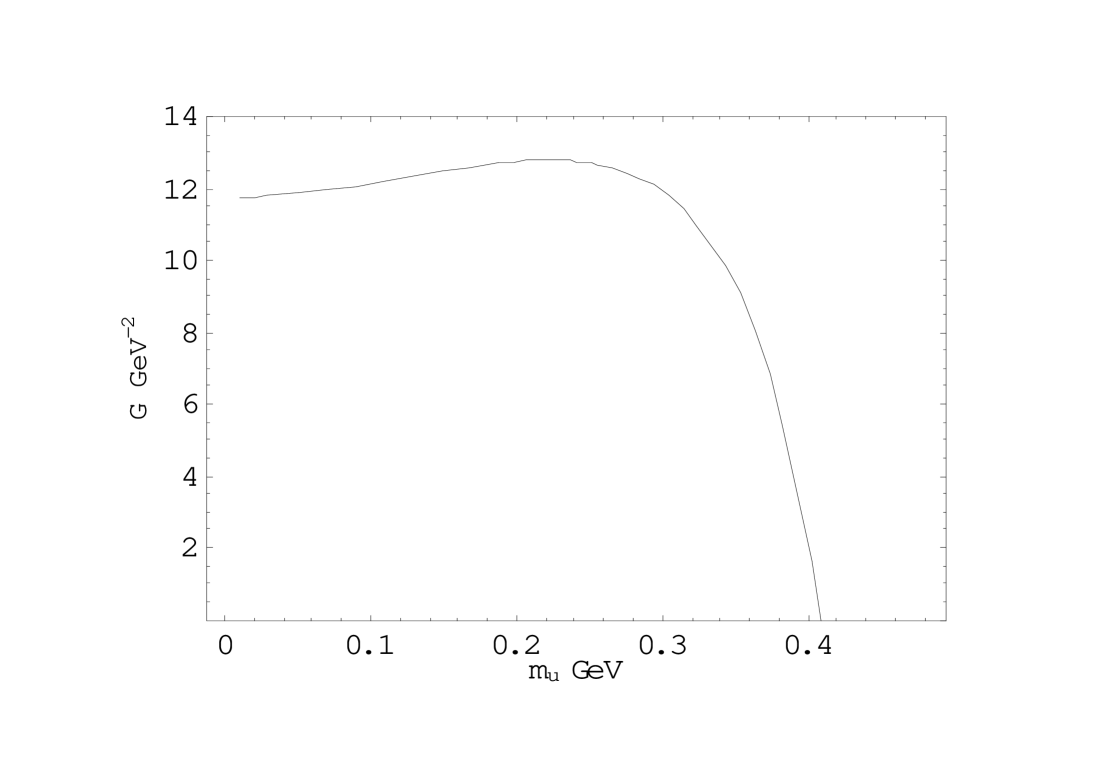
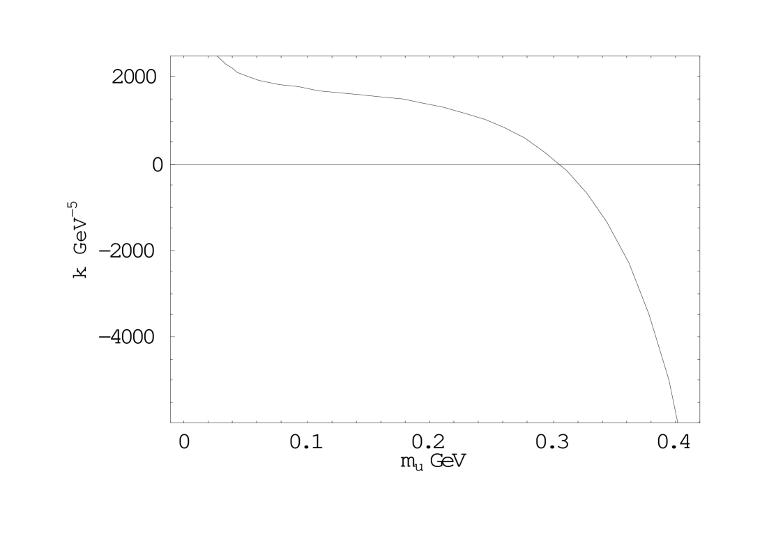
FIG. 1.: The couplings $G$ (left panel) and $\kappa$ (right panel) as functions of $m_{u}$ at fixed values of $m_{s}=572$ MeV and other parameters in Eq.(42). These curves show the typical $m_{u}$-dependence of the functions if one neglects the fluctuations term in Eq.(40).

$$e_{ai}=\frac{1}{2\sqrt{3}}\left(\begin{array}[]{ccc}\sqrt{2}&\sqrt{2}&\sqrt{2}\\ \sqrt{3}&-\sqrt{3}&0\\ 1&1&-2\end{array}\right),\qquad\omega_{ia}=\frac{1}{\sqrt{3}}\left(\begin{array}[]{ccc}\sqrt{2}&\sqrt{3}&1\\ \sqrt{2}&-\sqrt{3}&1\\ \sqrt{2}&0&-2\end{array}\right).$$ (39)

Here the index $a$ runs $a=0,3,8$ (for the other values of $a$ the corresponding matrix elements are equal to zero). We have also $h_{a}=e_{ai}h_{i}$, and $h_{i}=\omega_{ia}h_{a}$. Similar relations can be obtained for $\Delta_{i}$ and $\Delta_{a}$. In accordance with these notations we will use, for instance, that $h^{(1)}_{ci}=\omega_{ia}h^{(1)}_{ca}$.

A tadpole graphs calculation gives for the gap equations the following result

$$2h_{i}+\frac{3a\kappa}{8G^{2}}\left(h^{(2)}_{ab}-h^{(1)}_{ab}\right)A_{abc}h^{(1)}_{ci}=\frac{N_{c}}{2\pi^{2}}m_{i}J_{0}(m_{i}^{2})$$ (40)

where the left hand side is the contribution from (37) and the right hand side is the contribution of the quark loop from (11) with a regularized quadratically divergent integral $J_{0}(m^{2})$ being defined as

$$J_{0}(m^{2})=\int_{0}^{\infty}\frac{dt}{t^{2}}e^{-tm^{2}}\rho(t,\Lambda^{2}),\qquad\rho(t,\Lambda^{2})=1-(1+t\Lambda^{2})\exp(-t\Lambda^{2}).$$ (41)

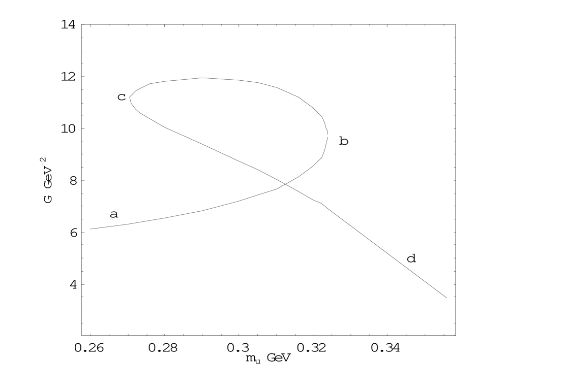
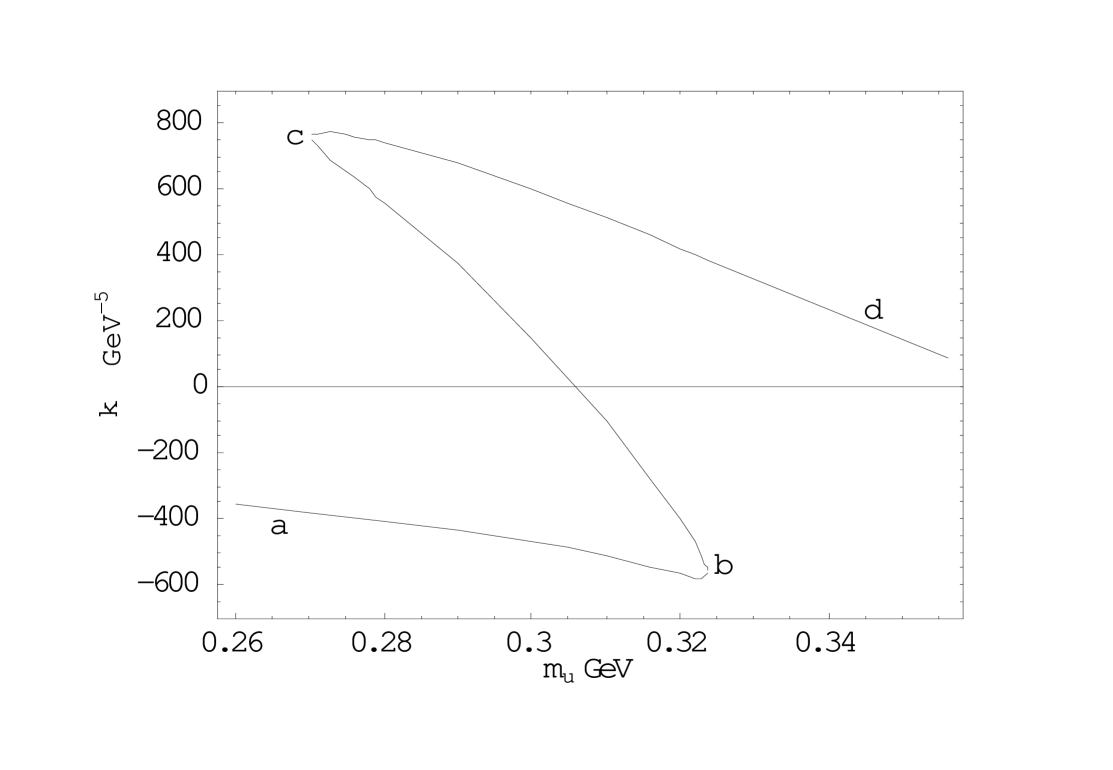
FIG. 2.: The couplings $G$ (left panel) and $\kappa$ (right panel) as functions of $m_{u}$ for the same (as in Fig.1) values of other fixed parameters and for the case when the fluctuations term in Eq.(40) is taken into account.

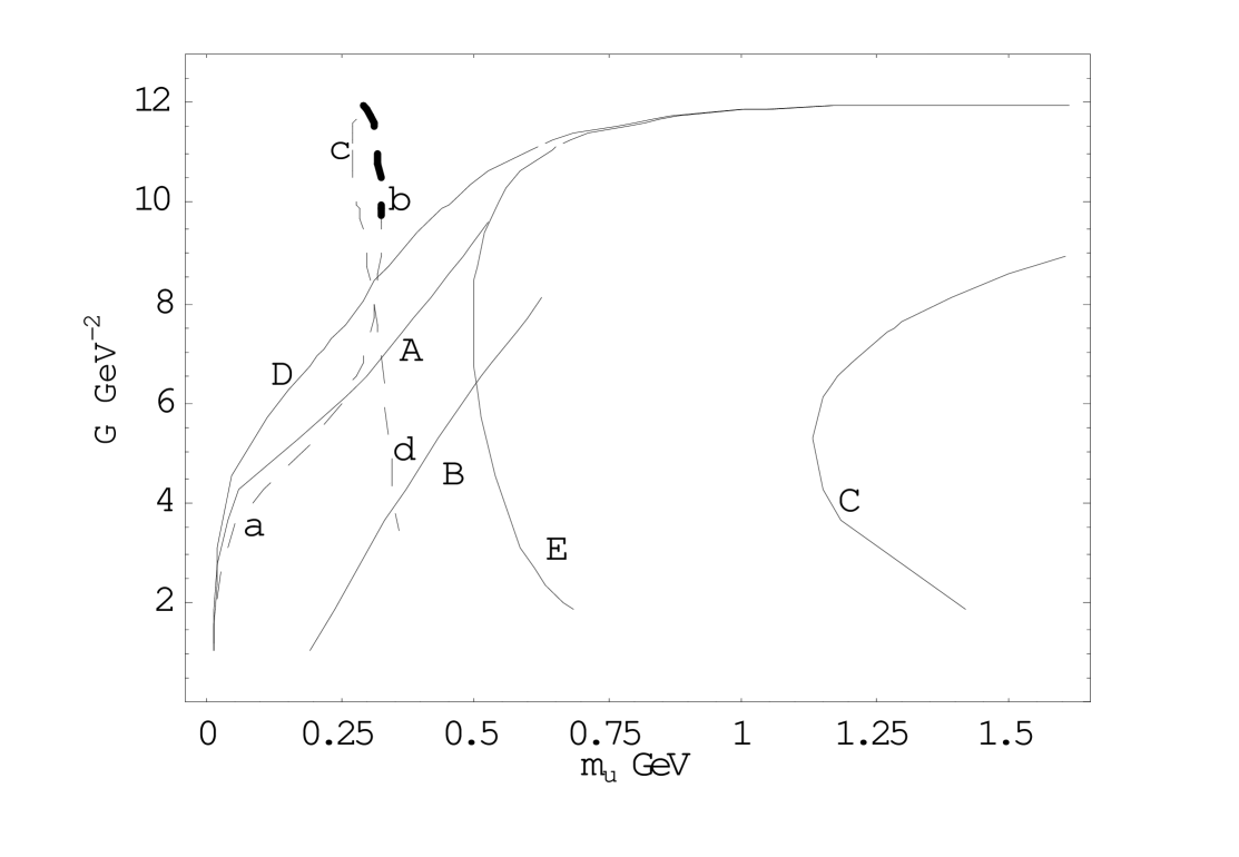
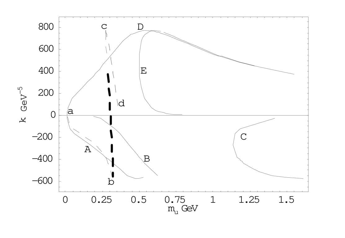
FIG. 3.: Different classes of $m_{u}$ solutions of the gap equations, including fluctuations, at fixed $G,\kappa$ values. Four branches of solutions, $A,B,C$ and $a-b$ stretch have negative $\kappa$. Three branches, $D,E$ and along $c-d$ arm correspond to positive $\kappa$. Bold dashes indicate that only one solution exists in this region of $G,\kappa$. See further details in text.

The second term on the left hand side of Eq.(40) is the correction resulting from the Gaussian integrals of the steepest descent method, comprising the effects of small fluctuations around the stationary path. If one puts for a moment $a=0$ in Eq.(40), and combines the result with Eqs.(38), one finds gap equations which are very similar to the ones obtained in [4] (see equation (2.12) therein). At fixed input parameters $G,\kappa,\Lambda$ of the model, the gap equations can be solved giving us the constituent quark masses $m_{i}$ as functions of the current quark masses, $m_{i}=m_{i}(\hat{m}_{j})$. Alternatively, by fixing $\hat{m}_{i}$, one can obtain from the gap equations the non-trivial solutions $m_{i}=m_{i}(G,\kappa,\Lambda)$. In particular, when $\hat{m}_{u}=\hat{m}_{d}$, these equations can be solved for $G$ and $\kappa$, giving expressions

$$G=\left(\frac{2\pi^{2}}{N_{c}}\right)\frac{m_{u}\Delta_{u}J_{0}(m^{2}_{u})-m_{s}\Delta_{s}J_{0}(m^{2}_{s})}{m_{u}^{2}J_{0}^{2}(m^{2}_{u})-m_{s}^{2}J_{0}^{2}(m^{2}_{s})},\qquad\kappa=\left(\frac{8\pi^{2}}{N_{c}}\right)^{2}\frac{m_{s}\Delta_{u}J_{0}(m^{2}_{s})-m_{u}\Delta_{s}J_{0}(m^{2}_{u})}{m_{u}J_{0}(m_{u}^{2})[m_{u}^{2}J_{0}^{2}(m^{2}_{u})-m_{s}^{2}J_{0}^{2}(m^{2}_{s})]}.$$ (42)

In Fig.1 we plot the curves of $G$ and $\kappa$ versus $m_{u}$ keeping constant $\Lambda=0.87\ \mbox{GeV},\ m_{s}=572\ \mbox{MeV},\ \hat{m}_{s}=200\ \mbox{MeV},\ \hat{m}_{u}=6\ \mbox{MeV}$. One can readily see that at given values for $(m_{u},m_{s})$ the curves yield unique values of $(G,\kappa)$, i.e. the vacuum state is well-defined in this case.

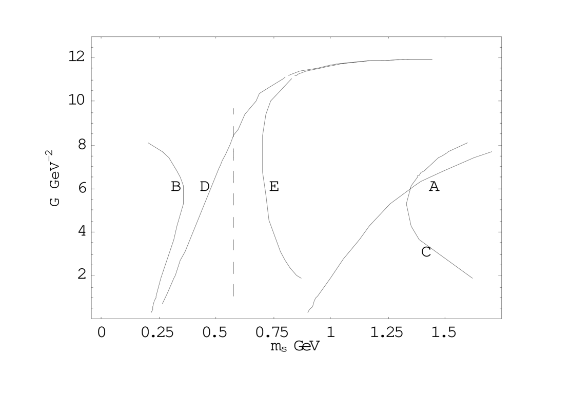
FIG. 4.: The same as in figure 3 for the $m_{s}$ solutions. The dashes are the constant $m_{s}$ corresponding to the $abcd$ curve of Figs. 2 and 3.

Let us consider now the general case which we have when $a>0$ in Eq.(40). To illustrate the qualitative difference with the previous case we put for definiteness $a=1$ and look again for the solutions $G=G(m_{u})$ and $\kappa=\kappa(m_{u})$ with the same set of fixed parameters. The corresponding curves are plotted in Fig.2. If the mass $m_{u}$ is sufficiently low that $m_{u}<m_{u}^{(min)}$, (in the figures denoted by the region left the turning point $c$) or sufficiently high that $m_{u}^{(max)}<m_{u}<m_{s}$, (in the figures denoted by the region right to the turning point $b$), then there exists again a single solution with unique values of $(G,\kappa)$. However, there is now a region for $m_{u}$ in which $m_{u}^{(min)}<m_{u}<m_{u}^{(max)}$, where three values of couplings $(G,\kappa)$ are possible.

Conversely, one can study the solutions: $m_{u}=m_{u}(G,\kappa),\ m_{s}=m_{s}(G,\kappa$ at fixed values of input parameters: $\Lambda,\hat{m}_{u}=\hat{m}_{d},\hat{m}_{s})$. As starting input values for the couplings $G$ and $\kappa$ in the gap equations we take the ones already determined along the path $abcd$ shown in Fig.2, obtained at a constant value of the strange quark mass, $m_{s}=572$ MeV. For a chosen value of the set $(G,\kappa)$ we then search for further solutions $(m_{u},m_{s})$ of the Eq.(40), displaying results in Fig.3 for $m_{u}$ and in Fig.4 for $m_{s}$, correspondingly. The dashed curves are the repetition of the solutions encountered in Fig.2. The bold dashes in Fig.3 indicate that we only find this one solution at fixed values of $G,\kappa$. Combining the information of Figs.3 and 4, one sees that one has up to four solutions at fixed $G,\kappa$. Indeed, travelling along the original path $abcd$ one observes the following: the branch $ab$ is accompanied by three other branches, marked as $A,B$ and $C$ which belong to the same class of solutions. One sees that these solutions have negative $\kappa$ values. From the turning point $b$ until the maximum value of $G$ (and corresponding $\kappa$) (bold dashes) we have no other solutions to the gap equations, as already stated. From this maximum $G$ value to the turning point $c$ and further along the $cd$ arm we encounter further two branches, denoted by $D$ and $E$ to the solutions of Eqs.(40) with same $G,\kappa$. They are positive $\kappa$ solutions.

This very rich structure of the vacuum solutions implies the possibility of having several different values of the quark condensates for the same $G,\kappa$ parameters, embracing also the possibility which has been considered in connection with generalized chiral perturbation theory (see e.g. section 4 in [10]). We give here only a few examples. At $G=4.54\ \mbox{GeV}^{-2},\kappa=153.04\ \mbox{GeV}^{-5}$ we have three solutions. The solution $m_{u}=346\ \mbox{MeV},m_{s}=572\ \mbox{MeV}$, on the $cd$ arm has the quark condensates $<\bar{u}u>^{1/3}=-236.8\ \mbox{MeV}$, $<\bar{s}s>^{1/3}=-183.5\ \mbox{MeV}$ and the ratio $R={(<\bar{s}s>/<\bar{u}u>)}^{1/3}=0.775$; the second solution, on the $E$ branch with $m_{u}=535\ \mbox{MeV},m_{s}=732\ \mbox{MeV}$ has condensates $<\bar{u}u>^{1/3}=-249\ \mbox{MeV}$, $<\bar{s}s>^{1/3}=-183\ \mbox{MeV}$ and the ratio $R=0.738$; the third solution, located at the $D$ branch with $m_{u}=46\ \mbox{MeV},m_{s}=418\ \mbox{MeV}$ has condensates $<\bar{u}u>^{1/3}=-131\ \mbox{MeV}$, $<\bar{s}s>^{1/3}=-172\ \mbox{MeV}$ and $R=1.313$. We chose the next example at $G=8.126\ \mbox{GeV}^{-2},\kappa=-544.81\ \mbox{GeV}^{-5}$, where there are four solutions. The solution $m_{u}=316\ \mbox{MeV},m_{s}=572\ \mbox{MeV}$, on the $ab$ arm has the quark condensates $<\bar{u}u>^{1/3}=-233\ \mbox{MeV}$, $<\bar{s}s>^{1/3}=-184\ \mbox{MeV}$ and $R=0.787$; the second solution, on the $B$ branch with $m_{u}=624\ \mbox{MeV},m_{s}=205\ \mbox{MeV}$ has condensates $<\bar{u}u>^{1/3}=-249\ \mbox{MeV}$, $<\bar{s}s>^{1/3}=-56.7\ \mbox{MeV}$ and $R=0.227$; the third solution, located at the $A$ branch with $m_{u}=421\ \mbox{MeV},m_{s}=1.84\ \mbox{GeV}$ has condensates $<\bar{u}u>^{1/3}=-14.4\ \mbox{MeV}$, $<\bar{s}s>^{1/3}=-86\ \mbox{MeV}$ and $R=0.353$. The fourth solution, on the $C$ branch, with $m_{u}=1.394\ \mbox{GeV},m_{s}=1.594\ \mbox{GeV}$ has condensates $<\bar{u}u>^{1/3}=-230\ \mbox{MeV}$, $<\bar{s}s>^{1/3}=-120\ \mbox{MeV}$ and the ratio $R=0.524$. As a final example we take the solutions at $G=11.96\ \mbox{GeV}^{-2}\simeq G_{max},\kappa=371.491\ \mbox{GeV}^{-5}$, where the branches $D$ and $E$ emerge and are very close to each other with $m_{u}=1.56\ \mbox{GeV},m_{s}=1.72\ \mbox{GeV}$. The corresponding condensates are $<\bar{u}u>^{1/3}=-224\ \mbox{MeV}$, $<\bar{s}s>^{1/3}=-105\ \mbox{MeV}$ and $R=0.467$. The other solution is at the path $bc$ with $m_{u}=290\ \mbox{MeV},m_{s}=572\ \mbox{MeV}$ with condensates $<\bar{u}u>^{1/3}=-229\ \mbox{MeV}$, $<\bar{s}s>^{1/3}=-184\ \mbox{MeV}$ and $R=0.8$.

To summarize, we have found that in the presence of the ’t Hooft interaction, treated beyound the lowest order SPA, several solutions to the gap equations are possible at some range of input parameters, i.e. the same values of $G,\kappa,\Lambda,\hat{m}_{i}$ lead to different sets of constituent quark masses $(m_{u},m_{s})$ and, therefore, to different values of the quark condensates. A quite different scenario emerges for the hadronic vacuum, which can now be multivalued. It makes our result essentially different from the ones obtained in [6, 4]. These findings must be further analysed in order to establish which of the extrema correspond to minima or maxima of the effective potential. This step will be done elsewhere in conjunction with the determination of the meson mass spectrum, as it also requires dealing with the terms with two powers of the meson fields in the ansatz of solutions Eq.(22) and in the related Lagrangian (28).

IV Concluding remarks

The purpose of this work has been twofold. Firstly we have developed the technique which is necessary to go beyound the lowest order SPA in the problem of the path integral bosonization of the ’t Hooft six quark interaction. We have shown how the pre-exponential factor, connected with the steepest descent approach and which is responsible for the quantum fluctuations around the classical path, can be treated exactly, order by order, in a scheme of increasing number of mesonic fields, while preserving all chiral symmetry requirements. This technique is rather general and can be readily used in other applications. Second, we have explored with considerable detail the implications of taking the quantum fluctuations in account in the description of the hadronic vacuum. A very complex multivalued vacuum emerges at fixed values of the input parameters $G$, $\kappa$, $\Lambda$ and current quark masses. We encountered several classes of solutions. Searching in an interval of constituent quark masses from zero to $\simeq 3$GeV, we found $G,\kappa$, regions caracterized by one, three and four solutions. The multiple vacua may have very interesting physical consequences and applications.

REFERENCES

- [1] A. M. Polyakov, Phys. Lett. B 59 (1975) 82; Nucl. Phys. B 121 (1977) 429. A. A. Belavin, A. M. Polyakov, A. Schwartz and Y. Tyupkin, Phys. Lett. B 59 (1975) 85. G. ’t Hooft, Phys. Rev. Lett. 37 (1976) 8; Phys. Rev. D 14 (1976) 3432. C. Callan, R. Dashen and D. J. Gross, Phys. Lett. B 63 (1976) 334. R. Jackiw and C. Rebbi, Phys. Rev. Lett. 37 (1976) 172. S. Coleman, “The uses of instantons” Erice Lectures, 1977.
- [2] D. Diakonov, “Chiral symmetry breaking by instantons”, Lectures at the Enrico Fermi School in Physics, Varenna, June 27 - July 7 (1995); hep-ph/9602375.
- [3] Y. Nambu, G. Jona-Lasinio, Phys. Rev. 122 (1961) 345; 124 (1961) 246; V. G. Vaks, A. I. Larkin ZhETF 40 (1961) 282.
- [4] V. Bernard, R. L. Jaffe, U.-G. Meißner, Nucl. Phys. B 308 (1988) 753.
- [5] T. Kunihiro and T. Hatsuda, Phys. Lett. B 206 (1988) 385. T. Hatsuda, Phys. Lett. B 213 (1988) 361. Y. Kohyama, K. Kubodera and M. Takizawa, Phys. Lett. B 208 (1988) 165. M. Takizawa, Y. Kohyama and K. Kubodera, Prog. Theor. Phys. 82 (1989) 481.
- [6] H. Reinhardt and R. Alkofer, Phys. Lett. B 207 (1988) 482.
- [7] D. Diakonov, “Chiral quark-soliton model”, Lectures at the Advanced Summer School on non-perturbative field theory, Peniscola, Spain, June 2-6 (1997); hep-ph/9802298.
- [8] A.A. Osipov and B. Hiller, Phys. Rev. D 62 (2000) 114013; idem Phys. Rev. D 63 (2001) 094009.
- [9] R. Jackiw, Int. J. Mod. Phys. B 14 (2000) 2011; hep-th/9903044.
- [10] H. Leutwyler, Talk given at the Conf. on Fundamental Interactions of Elem. Part., ITEP, Moscow, Russia, 1995, CERN-TH/96-25; hep-ph/9602255.