Neutrino decay confronts the SNO data

Abstract

We investigate the status of the neutrino decay solution to the solar neutrino problem in the context of the recent results from Sudbury Neutrino Observatory (SNO). We present the results of global $\chi^{2}$-analysis for both two and three generation cases with one of the mass states being allowed to decay and include the effect of both decay and mixing. We find that the Large Mixing Angle (LMA) region which is the currently favoured solution of the solar neutrino problem is affected significantly by decay. We present the allowed areas in the $\Delta m^{2}-\tan^{2}\theta$ plane for different allowed values of $\alpha$ and examine how these areas change with the inclusion of decay. We obtain bounds on the decay constant $\alpha$ in this region which implies a rest frame life time $\tau_{0}/m_{2}>8.7\times 10^{-5}$ sec/eV for the unstable neutrino state. We conclude that the arrival of the neutral current results from SNO further disfavors the neutrino decay solution to the solar neutrino problem leaving a very small window for the decay constant $\alpha$ which could still be allowed.

1 Introduction

The comparison of the SNO charged current (CC) measurments with their neutral current (NC) rate establishes oscillations to active neutrino flavor at the $5.3\sigma$ level [1]. The inclusion of Super-Kamiokande (SK) electron scattering (ES) rate [2] with SNO confirms transitions to active flavors at more than $5.5\sigma$ level. In other words SNO rules out the possibility of having a purely sterile component in the solar neutrino beam at the $5.5\sigma$ level. However presence of sterile components in the beam is not entirely ruled out. Transition to mixed states is still allowed with $<32\%(65\%)$ sterile mixture at the $1\sigma(2\sigma)$ level [3, 4, 5]. One of the scenarios in which one can have a final sterile state is neutrino decay. The aim of this paper is to investigate the status of the neutrino decay solution to the solar neutrino problem with the incorporation of the SNO data. We deal with both two generation and three generation cases. For the latter we consider three flavor mixing between $\nu_{e}$, $\nu_{\mu}$ and $\nu_{\tau}$ with mass eigenstates $\nu_{1}$, $\nu_{2}$ and $\nu_{3}$ with the assumed mass hierarchy as $m^{2}_{1}<m^{2}_{2}<m^{2}_{3}$. The lightest neutrino mass state is assumed to have lifetime much greater than the Sun-Earth transit time and hence can be taken as stable. Whereas the heavier mass states $\nu_{2}$ and $\nu_{3}$ may be unstable. But the CHOOZ data [6] constrains the mixing matrix element U_e3 to a very small value which implies very small mixture of the $\nu_{3}$ state to the $\nu_{e}$ state produced in Sun. So the instability of the $\nu_{3}$ state has hardly any effect on solar neutrino survival probability, and to study the effect of decay on solar neutrinos for simplicity we can consider only the second mass state $\nu_{2}$ to be unstable.

There are two kinds of models of non-radiative decays of neutrinos

• If neutrinos are Dirac particles one has the decay channel $\nu_{2}\rightarrow\bar{\nu}_{1R}+\phi$, where ${\bar{\nu}}_{1R}$ is a right handed singlet and $\phi$ is an iso-singlet scaler [7]. Thus all the final state particles are sterile.

• If neutrinos are Majorana particles, the decay mode is $\nu_{2}\rightarrow\bar{\nu}_{1}+J$, where $\bar{\nu}_{1}$ interacts as a $\bar{\nu}_{e}$ with a probability $|U_{e1}|^{2}$ and J is a Majoron [8].

In both scenarios the rest frame lifetime of $\nu_{2}$ is given by [9]

$$\tau_{0}=\frac{16\pi}{g^{2}}\frac{m_{2}(1+m_{1}/m_{2})^{-2}}{\mbox{$\Delta{m}^{2}$~{}}}$$ (1)

where $g$ is the coupling constant and $\Delta m^{2}(=m_{2}^{2}-m_{1}^{2}$) is the mass squared difference between the states involved in the decay process. If a neutrino of energy E decays while traversing a distance $L$ then the decay term exp(-$\alpha L/E$) gives the fraction of neutrinos that decay. $\alpha$ is the decay constant and is related to $\tau_{0}$ as $\alpha=m_{2}/\tau_{0}$.

For the Sun-Earth distance of $1.5\times 10^{11}$ m, and for a typical neutrino energy of 10 MeV one starts getting appreciable decay for $\alpha\sim 10^{-12}$ eV². For lower values of $\alpha$ the exp(-$\alpha L/E)$ term goes to 1 signifying no decay while for $\alpha$ $>$ $10^{-10}$ eV² the exponential term goes to zero signifying complete decay of the unstable neutrinos. Assuming $m_{2}>>m_{1}$ the equation (1) can be written as

$$g^{2}\mbox{$\Delta{m}^{2}$~{}}\sim 16\pi\alpha$$ (2)

If we now incorporate the bound $g^{2}<4.5\times 10^{-5}$ as obtained from K decay modes [10] we get the bound $\Delta m^{2}>10^{6}\alpha$. This gives the range $\Delta m^{2}\stackrel{{\scriptstyle>}}{{\sim}}10^{-6}$ eV² for which we can have appreciable decay.

Neutrino decay in the context of the solar neutrino problem has been considered earlier in [7, 8, 11] and more recently in [12, 13, 14]. After the declaration of the SNO CC data last year [15], bounds on the decay constant $\alpha$ have been obtained from the data on total rates [16] as well as from SK spectrum data [17]. However with the declaration of the recent SNO neutral current results [1] we expect to have a better handle on the sterile admixture in the solar neutrino beam and hence tighter constraints on the decay constant $\alpha$. The statistical analysis for the two-generation oscillation solution for stable neutrinos with the global solar neutrino data including the recent results of the SNO experiment can be found in [3, 18, 19]. In this paper we consider the possibility for unstable neutrino states and do a combined global satistical analysis of the solar neutrino data including the total rates from the Cl and Ga experiments [20], the zenith-angle recoil energy spectrum from SK [2] and the combined (CC+ES+NC) day-night energy spectrum from SNO [1]. We do our analysis for both two and three generation scenarios. We include the results of the CHOOZ experiment [6] in our three generation analysis.

In section 2 we briefly present the survival probability for the solar neutrinos with one of the components unstable. In section 3 we first find the constraints on $\alpha$ coming from the global solar neutrino data within a two-generation framework. We argue that decay of solar neutrinos is largely disfavored as a result of the inclusion of the SNO day-night spectrum. We next extend our analysis to include the third neutrino flavor and present bounds on $\alpha$, $\Delta m^{2}_{21}$ and $\tan^{2}\theta_{21}$ for different allowed values of $\theta_{13}$, from a $\chi^{2}$ analysis which includes both the global solar neutrino data as well as the CHOOZ data. We end with conclusions in section 4.

2 Formalism

The three-generation mixing matrix relating the mass and flavour eigenstates are given as

$$U = R_{23}R_{13}R_{12}$$ (3)

$$= \pmatrix{c_{13}c_{12}&s_{12}c_{13}&s_{13}\cr-s_{12}c_{23}-s_{23}s_{13}c_{12}&c_{23}c_{12}-s_{23}s_{13}s_{12}&s_{23}c_{13}\cr s_{23}s_{12}-s_{13}c_{23}c_{12}&-s_{23}c_{12}-s_{13}s_{12}c_{23}&c_{23}c_{13}\cr}$$

where we neglect the CP violation phases.

Allowing for the possibility of decay of the second mass eigenstate the probability of getting a neutrino of flavour $f$ starting from an initial electron neutrino flavour is .

$$P_{ef} = {a_{e1}^{\odot}}^{2}|A_{1f}^{\oplus}|^{2}+{a_{e2}^{\odot}}^{2}|A_{2f}|^{2}e^{-\alpha(L-R_{\odot})/E}+{a_{e3}^{\odot}}^{2}|A_{3f}^{\oplus}|^{2}$$ (4)

$$+ 2a_{e1}^{\odot}a_{e2}^{\odot}e^{-\alpha(L-R_{\odot})/2E}Re[A_{1f}^{\oplus}A_{2f}^{\oplus*}e^{i(E_{2}-E_{1})(L-R_{\odot})}e^{i(\phi_{2,\odot}-\phi_{1,\odot})}]$$

where $E_{i}$ is the energy of the mass eigenstate $i$, $E$ is the energy of the neutrino beam, $\alpha$ is the decay constant, $L$ is the distance from the center of the Sun, $R_{\odot}$ is the radius of the Sun, $\phi_{i,\odot}$ are the phase inside the Sun and $a_{ei}^{\odot}$ is the amplitude of an electron state to be in the mass eigenstate $\nu_{i}$ at the surface of the Sun [22]

$${a_{ei}^{\odot}}^{2}=\sum_{j=1,2,3}X_{ij}{{U^{\odot}_{je}}}^{2}$$ (5)

where $X_{ij}$ denotes the non-adiabatic jump probability between the $i^{th}$ and $j^{th}$ states inside the Sun and $U_{je}^{\odot}$ denotes the mixing matrix element between the flavour state $\nu_{e}$ and the mass eigenstate $\nu_{j}$ in Sun. $A_{if}^{\oplus}$ denote the $\nu_{i}\rightarrow\nu_{f}$ transition amplitudes inside the Earth. We evaluate these amplitudes numerically by assuming the Earth to consist of two constant density slabs [22]. It can be shown that the square bracketed term containing the phases averages out to zero in the range of $\Delta{m}^{2}$ in which we are interested [23]. For further details of the calculation of the survival probability we refer to [22].

In the two generation limit the ${\nu_{e}}$ survival probability including Earth matter effects and decay can be expressed as [13]

$$P_{ee}=P_{ee}^{\rm day}+\frac{(\sin^{2}\theta-P_{2e})(P_{ee}^{\rm day}+e^{-2\alpha(L-R_{\odot})/E}(P_{ee}^{\rm day}-1))}{\cos^{2}\theta-\sin^{2}\theta e^{-2\alpha(L-R_{\odot})/E}}$$ (6)

where $P_{2e}$ is the transition probability of $\nu_{2}\rightarrow\nu_{e}$ at the detector while $P_{ee}^{\rm day}$ is the day-time survival probability (without Earth matter effects) for ${\nu_{e}}$ and is given by [13]

$$P_{ee}^{\rm day} = \cos^{2}\theta[P_{J}\sin^{2}\theta_{M}+(1-P_{J})\cos^{2}\theta_{M}]$$ (7)

$$+\sin^{2}\theta[(1-P_{J})\sin^{2}\theta_{M}+\cos^{2}\theta_{M}P_{J}]e^{-2\alpha(L-R_{\odot})/E}$$

where $P_{J}$ is the non-adiabatic level jumping probability between the two mass eigenstates for which we use the standard expression from [24] and $\theta_{M}$ is the matter mixing angle given by

$$\tan 2\theta_{M}=\frac{\Delta m^{2}\sin 2\theta}{\Delta m^{2}\cos 2\theta-2\sqrt{2}G_{F}n_{e}E}.$$ (8)

$n_{e}$ being the ambient electron density, $E$ the neutrino energy, and $\Delta{m}^{2}$ (= ${m_{2}^{2}-m_{1}^{2}}$) the mass squared difference in vacuum.

From eq.(7) we note that the decay term appears with a $\sin^{2}\theta$ and is therefore appreciable only for large enough $\theta$. Thus we expect the effect of decay to be maximum in the LMA region. This can also be understood as follows. The $\nu_{e}$ are produced mostly as $\nu_{2}$ in the solar core. In the LMA region the neutrinos move adiabatically through the Sun and emerge as $\nu_{2}$ which eventually decays. For the SMA region on the other hand $P_{J}$ is non-zero and $\nu_{e}$ produced as $\nu_{2}$ cross over to $\nu_{1}$ at the resonance and come out as a $\nu_{1}$ from the solar surface. Since $\nu_{1}$ is stable, decay does not affect this region.

3 Analysis of data and results

3.1 Bounds from two-generation analysis

First we use the standard $\chi^{2}$ minimisation procedure and determine the $\chi^{2}_{min}$ and the best-fit values of the oscillation and decay parameters, in a two flavor mixing scenario. Details of our statistical analysis procedure, including the definition of the $\chi^{2}$ and the correlated error matrix are given in Appendix A. We incorporate the total rate in Cl and Ga, the zenith-angle spectrum data of SK and the SNO day-night spectrum. We find that the global best-fit comes in the LMA region with the decay constant $\alpha=0$ and $\tan^{2}\theta=0.41,\Delta m^{2}=6.06\times 10^{-5}$eV² [25].

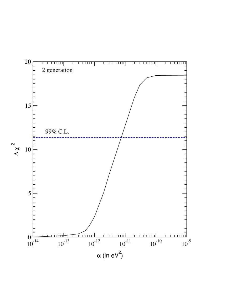
Figure 1: $\Delta\chi^{2}(=\chi^{2}-\chi^{2}_{min}$) vs decay constant $\alpha$, for two-generations. Also shown is the 99% C.L. limit for three-parameters.

In figure 1 we plot the $\Delta\chi^{2}$ ($=\chi^{2}-\chi^{2}_{min}$) for the two generation neutrino decay scenario, against the decay constant $\alpha$, keeping $\Delta m^{2}$ and $\tan^{2}\theta$ free. The figure shows that the fit becomes worse with increasing value of the decay constant. We remind the reader that neutrino decay is important only for LMA and for each value of $\alpha$ on this curve the minimum $\chi^{2}$ comes with $\Delta m^{2}$ and $\tan^{2}\theta$ in the LMA region. The inclusion of the SNO data in the global solar neutrino analysis improves the fit in the LMA region for stable neutrinos. Hence for small values of $\alpha$ where neutrinos can be taken as almost stable, the inclusion of the SNO data gives a better fit. However as $\alpha$ increases the neutrino decay leads to more sterile components in the final state – which is disfavoured by the SNO/SK combination and the fit worsens with SNO included. As is seen from figure 1 the global solar neutrino data put an upper bound on the decay constant – $\alpha<7.55\times 10^{-12}$eV² at 99% C.L., when $\Delta m^{2}$ and $\theta$ are allowed to take on any value. Before the declaration of the SNO results the bound on $\alpha$ from combined analysis of Cl, Ga and SK data was $\alpha<3.5\times 10^{-11}$ eV² [13]. Thus the inclusion of the recent SNO results have further tightened the noose on the fraction of neutrinos decaying on their way from the Sun to Earth and neutrino decay is now barely allowed.

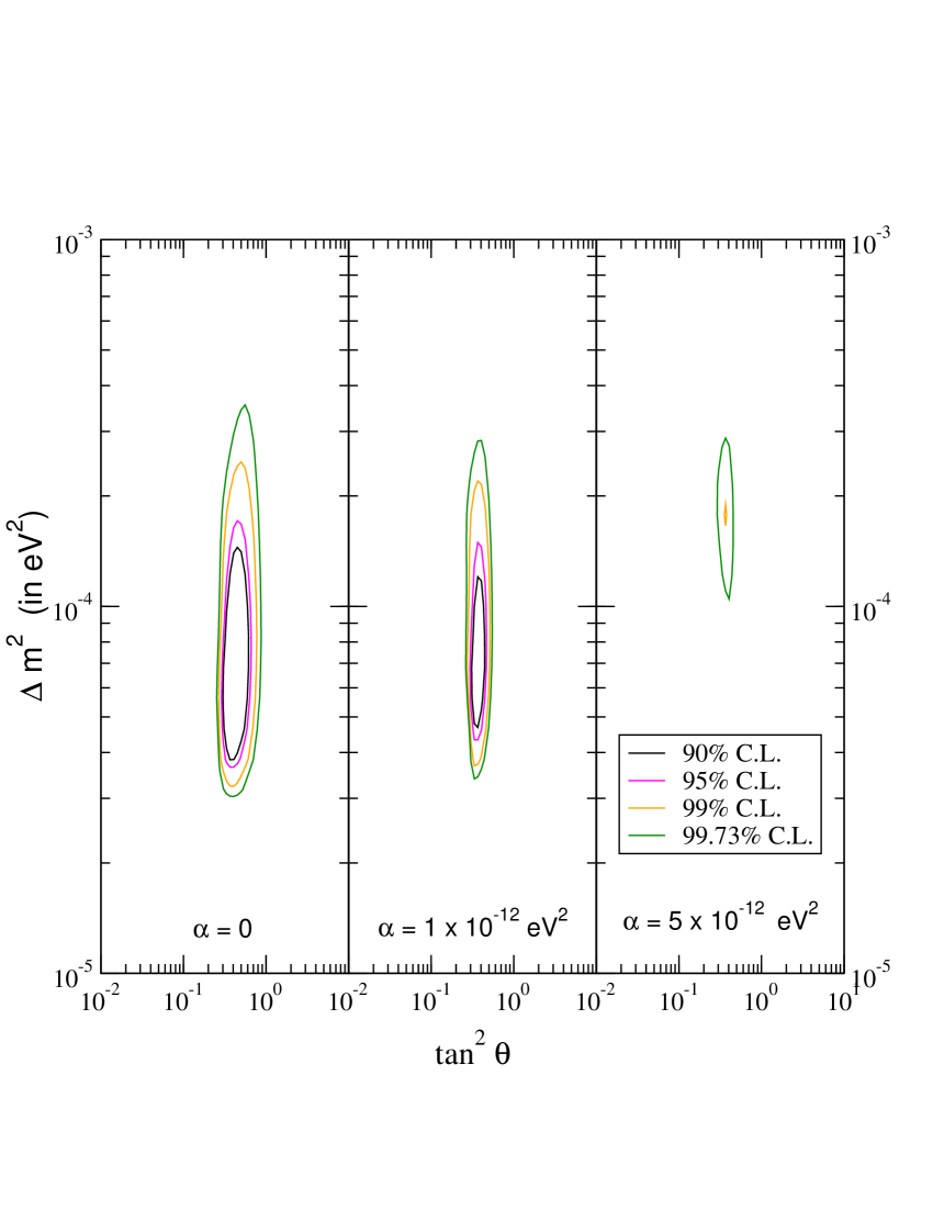
Figure 2: The 90, 95, 99 and 99.73% C.L. allowed area from the two-generation global analysis of the total rates in Cl and Ga, the SK zenith angle energy spectrum data and the SNO day-night spectrum in presence of decay and oscillation. The C.L. contours are for $\Delta\chi^{2}$ corresponding to three parameters.

In figure 2 we plot the allowed areas in the $\Delta m^{2}-\tan^{2}\theta$ plane for different allowed values of the decay constant $\alpha$ for a two flavor scenario and with global data including SNO. The figure shows that the allowed area in the LMA region is reduced as $\alpha$ increases. As $\alpha$ increases the spectral distortion increases and the effect is more for higher(lower) values of $\tan^{2}\theta$($\Delta m^{2}$) [13]. Since both the SK as well as the SNO spectra are consistent with no energy distortion, these regions get disallowed with increasing $\alpha$. Spectral distortion due to decay is less for the high $\Delta m^{2}$. However these values for the $\Delta m^{2}$ are now disfavored at more than $3\sigma$ by SNO since the values for the ${}^{8}B$ flux required to explain the suppression in SK and SNO CC measurements are much lower than those consistent with the SNO NC observation. In addition the low energy neutrinos relevant for Ga experiment decay more making the fit to the total rates worse.

As discussed earlier, for small values of mixing angles the fraction of the decaying component in the $\nu_{e}$ beam ($\sim\sin^{2}\theta$) being very small decay does not have much effect. Hence no new feature is introduced in the SMA region because of decay and it remains disallowed by the global data. On the other hand, in the LOW region though mixing is large, due to small $\Delta m^{2}$ any appreciable decay over the Sun-Earth distance is not obtained, if the bound on the coupling constant from K-decay [10] is to be accounted for. Therefore, LOW region in the parameter space remains unaffected by the unstable $\nu_{2}$ state, and we do not show it explicitly in figure 2.

3.2 Bounds from three-generation analysis

Next we investigate the impact of the unstable $\nu_{2}$ mass state on the three flavor oscillation scenario with $\Delta m_{21}^{2}=\Delta m_{\odot}^{2}$ and $\Delta m_{31}^{2}=\Delta m_{CHOOZ}^{2}\simeq\Delta m_{atm}^{2}=\Delta m_{32}^{2}.$ For the three generation case the $\chi^{2}$ is defined as

$$\chi^{2}=\chi^{2}_{solar}+\chi^{2}_{chooz}$$ (9)

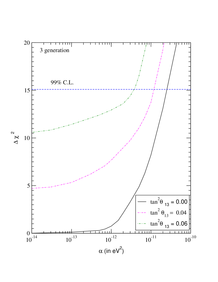
Figure 3: The $\Delta\chi^{2}(=\chi^{2}-\chi^{2}_{min}$) vs decay constant $\alpha$ for the three generation case for various fixed values of $\theta_{13}$. The other parameters are allowed to take any value.

The $\chi^{2}_{solar}$ is defined in Appendix A while for the expression of $\chi^{2}_{chooz}$ we refer the reader to [22]. In figure 3 we plot the $\Delta\chi^{2}(=\chi^{2}-\chi^{2}_{min})$ vs $\alpha$ for various fixed values of $\theta_{13}$ allowing the other parameters to take arbitrary values. $\Delta m_{31}^{2}$ is varied within the range [1.5 - 6.0]$\times$ 10^-3 eV² as obtained from a combined analysis of atmospheric and CHOOZ data [28, 29]. This figure indicates the allowed range of $\alpha$ for a fixed $\theta_{13}$. As $\theta_{13}$ increases the contribution from $\chi^{2}_{chooz}$ increases shifting the plots upwards. Consequently the curve corresponding to higher $\tan^{2}\theta_{13}$ crosses the 99% C.L. limit at a lower $\alpha$ and a more stringent bound is obtained as compared to smaller $\tan^{2}\theta_{13}$ cases.

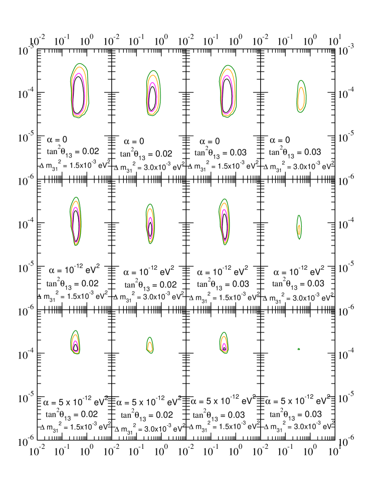
Figure 4: The 90, 95, 99 and 99.73% C.L. allowed area from the three-generation analysis of the global data in presence of decay and oscillation.

In figure 4 we plot the allowed areas in the $\tan^{2}\theta_{12}-\Delta m_{21}^{2}$ plane for different sets of values of $\tan^{2}\theta_{13}$ and $\Delta m_{31}^{2}$ at different values of $\alpha$. For fixed values of $\tan^{2}\theta_{13}$ and $\Delta m^{2}_{31}$ the allowed area decreases with increasing $\alpha$ because of increased spectral distortion and transition of the solar neutrinos to sterile components. At any given $\alpha$ the allowed area shrinks with the increase of $\tan^{2}\theta_{13}$ and $\Delta m_{31}^{2}$. This is again an effect of the CHOOZ data.

4 Conclusions

In this paper we have done a global $\chi^{2}$ analysis of the solar neutrino data assuming neutrino decay. We incorporate the full SNO (CC+ES+NC) day-night spectrum data. We present results for both two and three generation scenarios. We find that the best fit is obtained in the LMA region with the decay constant $\alpha$ zero i.e. for the no decay case. We had pointed earlier [12, 13] that the decay scenario was in conflict with the data on total rates because it suppresses low energy neutrinos more than the high energy ones. However decay also predicts distortion of the neutrino energy spectrum and presence of sterile components in the resultant neutrino beam, both of which are severely disfavored by the recent results from SNO and SK. For the two generation case the bound at 99% C.L. on $\alpha$ that one gets after including the SNO data is $\alpha\leq 7.55\times 10^{-12}$eV². This corresponds to a rest frame lifetime $\tau_{0}/m_{2}>8.7\times 10^{-5}s/eV$. This is consistent with astrophysics and cosmology. The effect of decay is not important in the SMA region because the decaying fraction in the solar $\nu_{e}$ beam goes as $\sin^{2}\theta$ and this region remains disallowed. There is no change in the allowed areas in the LOW region also because of eq. (2) and the bounds on the coupling constant from K decays which restricts $\Delta m^{2}\stackrel{{\scriptstyle>}}{{\sim}}10^{-6}$ eV² and decay over the Sun-Earth distance does not take place in the LOW region. The three generation analysis gives stronger bounds on $\alpha$ for non-zero $\theta_{13}$. In conclusion, the inclusion of the recent SNO data severely constrains decay of the solar neutrinos such that they are largely disfavored. However nonzero values of $\alpha$ remain allowed at the 99% C.L..

Appendix A The statistical analysis of the global solar data

We use the data on total rate from the Cl experiment, the combined rate from the Ga experiments (SAGE+GALLEX+GNO), the 1496 day data on the SK zenith angle energy spectrum and the combined SNO day-night spectrum data. We define the $\chi^{2}$ function in the “covariance” approach as

$$\chi^{2}=\sum_{i,j=1}^{N}(R_{i}^{\rm expt}-R_{i}^{\rm theory})(\sigma_{ij}^{2})^{-1}(R_{j}^{\rm expt}-R_{j}^{\rm theory})$$ (10)

where $N$ is the number of data points ($2+44+34=80$ in our case) and $(\sigma_{ij}^{2})^{-1}$ is the inverse of the covariance matrix, containing the squares of the correlated and uncorrelated experimental and theoretical errors. The only correlated error between the total rates of Cl and Ga, the SK zenith-energy spectrum and the SNO day-night spectrum data is the theoretical uncertainty in the ${}^{8}B$ flux. However we choose to keep the ${}^{8}B$ flux normalization $f_{B}$ a free parameter in the theory, to be fixed by the neutral current contribution to the SNO spectrum. We can then block diagonalise the covariance matrix and write the $\chi^{2}$ as a sum of $\chi^{2}$ for the rates, the SK spectrum and SNO spectrum.

$$\chi^{2}=\chi_{\rm rates}^{2}+\chi_{\rm SKspec}^{2}+\chi_{\rm SNOspec}^{2}$$ (11)

For $\chi^{2}_{\rm rates}$ we use $R_{\rm Cl}^{\rm expt}=2.56\pm 0.23$ SNU and $R_{\rm Ga}^{\rm expt}=70.8\pm 4.4$ SNU. The details of the theoretical errors and their correlations that we use can be found in [26, 31].

For the 44 bin SK zenith angle energy spectra we use the data and experimental errors given in [2]. SK divides it’s systematic errors into “uncorrelated” and “correlated” systematic errors. We take the “uncorrelated” systematic errors to be uncorrelated in energy but fully correlated in zenith angle. The “correlated” systematic errors, which are fully correlated in energy and zenith angle, include the error in the ${}^{8}B$ spectrum shape, the error in the energy resolution function and the error in the absolute energy scale. For each set of theoretical values for $\Delta m^{2}$, $\tan^{2}\theta$ and $\alpha$ we evaluate these systematic errors taking into account the relative signs between the different errors [18]. Finally we take an overall extra systematic error of $2.75\%$ fully correlated in all the bins [2].

Since it is not yet possible to identify the ES, CC and NC events separately in SNO, the SNO collaboration have made available their results as a combined CC+ES+NC data in 17 day and 17 night energy bins. For the null oscillation case they do give the CC and NC (and ES) rates [1] but firstly these rates would slightly change with the distortion of the ${}^{8}B$ neutrino spectrum from the Sun and secondly they are highly correlated. They work very well for studying theories with little or no energy distortion such as the LMA and LOW MSW solutions if the (anti)correlations between the CC and NC rates are taken into account and can be used to study the impact of the NC rate of SNO on the oscillation parameter space [3]. They can also be used to give insight into the ${}^{8}B$ flux and it’s suppression by analysing the SK and SNO CC and NC data in a model independent way [3]. However for theories like neutrino decay where we expect large spectral distortions they cannot be used. Hence we analyse the full day-night spectrum data in this paper by adding contributions from CC, ES and NC and comparing with the experimental results given in [1]. For the correlated spectrum errors and the construction of the covariance matrix we follow the method of “forward fitting” of the SNO collaboration detailed in [32].

References

- [1] Q. R. Ahmad et al. [SNO Collaboration], Phys. Rev. Lett. 89, 011301 (2002) [arXiv:nucl-ex/0204008] ; ; Q. R. Ahmad et al. [SNO Collaboration], Phys. Rev. Lett. 89, 011302 (2002) [arXiv:nucl-ex/0204009].
- [2] S. Fukuda et al. [Super-Kamiokande Collaboration], Phys. Lett. B 539, 179 (2002) [arXiv:hep-ex/0205075].
- [3] A. Bandyopadhyay, S. Choubey, S. Goswami and D. P. Roy, Phys. Lett. B 540, 14 (2002) [arXiv:hep-ph/0204286].
- [4] J. N. Bahcall, M. C. Gonzalez-Garcia and C. Pena-Garay, arXiv:hep-ph/0204194.
- [5] M. Maltoni, T. Schwetz, M. A. Tortola and J. W. Valle, arXiv:hep-ph/0207227. ; M. Maltoni, T. Schwetz, M. A. Tortola and J. W. Valle, arXiv:hep-ph/0207157.
- [6] M. Apollonio et al. [CHOOZ Collaboration], Phys. Lett. B 466, 415 (1999) [arXiv:hep-ex/9907037] ; M. Apollonio et al. [CHOOZ Collaboration], Phys. Lett. B 420, 397 (1998) [arXiv:hep-ex/9711002].
- [7] A. Acker, S. Pakvasa, S. F. Tuan and S. P. Rosen, Phys. Rev. D 43, 3083 (1991).
- [8] A. Acker, A. Joshipura and S. Pakvasa, Phys. Lett. B 285, 371 (1992).
- [9] A. Acker and S. Pakvasa, Phys. Lett. B 320, 320 (1994) [arXiv:hep-ph/9310207].
- [10] V. Barger, W.Y.Keung and S. Pakvasa, Phys. Lett. B192, 460 (1987).
- [11] R. S. Raghavan, X. G. He and S. Pakvasa, Phys. Rev. D 38, 1317 (1988).
- [12] S. Choubey, S. Goswami and D. Majumdar, Phys. Lett. B 484, 73 (2000) [arXiv:hep-ph/0004193].
- [13] A. Bandyopadhyay, S. Choubey and S. Goswami, Phys. Rev. D 63, 113019 (2001) [arXiv:hep-ph/0101273].
- [14] Chih-Kang Chou and M. Cho, Phys. Scripta 64, 197 (2001).
- [15] Q. R. Ahmad et al. [SNO Collaboration], Phys. Rev. Lett. 87, 071301 (2001) [arXiv:nucl-ex/0106015].
- [16] A. S. Joshipura, E. Masso and S. Mohanty, arXiv:hep-ph/0203181.
- [17] J. F. Beacom and N. F. Bell, Phys. Rev. D 65, 113009 (2002) [arXiv:hep-ph/0204111].
- [18] G. L. Fogli, E. Lisi, A. Marrone, D. Montanino and A. Palazzo, arXiv:hep-ph/0206162.
- [19] J. N. Bahcall, M. C. Gonzalez-Garcia and C. Pena-Garay, JHEP 0207, 054 (2002) [arXiv:hep-ph/0204314] ; P. C. de Holanda and A. Y. Smirnov, arXiv:hep-ph/0205241 ; A. Strumia, C. Cattadori, N. Ferrari and F. Vissani, Phys. Lett. B 541, 327 (2002) [arXiv:hep-ph/0205261].
- [20] B. T. Cleveland et al., Astrophys. J. 496, 505 (1998) ; J. N. Abdurashitov et al. [SAGE Collaboration], arXiv:astro-ph/0204245 ; W. Hampel et al. [GALLEX Collaboration], Phys. Lett. B 447, 127 (1999) ; E. Bellotti, Talk at Gran Sasso National Laboratories, Italy, May 17, 2002 ; T. Kirsten, Talk at Neutrino 2002, Munich, Germany, May 2002.
- [21] M. Lindner, T. Ohlsson and W. Winter, Nucl. Phys. B 607, 326 (2001) [arXiv:hep-ph/0103170].
- [22] A. Bandyopadhyay, S. Choubey, S. Goswami and K. Kar, Phys. Rev. D 65, 073031 (2002) [arXiv:hep-ph/0110307].
- [23] A. S. Dighe, Q. Y. Liu and A. Y. Smirnov, arXiv:hep-ph/9903329.
- [24] S. T. Petcov, Phys. Lett. B 200, 373 (1988).
- [25] S. Choubey, A. Bandyopadhyay, S. Goswami and D. P. Roy, arXiv:hep-ph/0209222.
- [26] A. Bandyopadhyay, S. Choubey, S. Goswami and K. Kar, Phys. Lett. B 519, 83 (2001) [arXiv:hep-ph/0106264] ; S. Choubey, S. Goswami and D. P. Roy, Phys. Rev. D 65, 073001 (2002) [arXiv:hep-ph/0109017] ; S. Choubey, S. Goswami, K. Kar, H. M. Antia and S. M. Chitre, Phys. Rev. D 64, 113001 (2001) [arXiv:hep-ph/0106168].
- [27] G. L. Fogli, E. Lisi, D. Montanino and A. Palazzo, Phys. Rev. D 64, 093007 (2001) [arXiv:hep-ph/0106247] ; J. N. Bahcall, M. C. Gonzalez-Garcia and C. Pena-Garay, JHEP 0108, 014 (2001) [arXiv:hep-ph/0106258] ; P. I. Krastev and A. Y. Smirnov, Phys. Rev. D 65, 073022 (2002) [arXiv:hep-ph/0108177] ; M. V. Garzelli and C. Giunti, JHEP 0112, 017 (2001) [arXiv:hep-ph/0108191].
- [28] M. C. Gonzalez-Garcia, M. Maltoni, C. Pena-Garay and J. W. Valle, Phys. Rev. D 63, 033005 (2001) [arXiv:hep-ph/0009350].
- [29] G. L. Fogli, E. Lisi, A. Marrone, D. Montanino and A. Palazzo, arXiv:hep-ph/0104221.
- [30] G. L. Fogli, G. Lettera, E. Lisi, A. Marrone, A. Palazzo and A. Rotunno, arXiv:hep-ph/0208026.
- [31] S. Goswami, D. Majumdar and A. Raychaudhuri, Phys. Rev. D 63, 013003 (2001) [arXiv:hep-ph/0003163]. ; S. Choubey, S. Goswami, N. Gupta and D. P. Roy, Phys. Rev. D 64, 053002 (2001) [arXiv:hep-ph/0103318].
- [32] SNO Collaboration, HOWTO use the SNO Solar Neutrino Spectral data at http://owl.phy.queensu.ca/sno/prlwebpage/.